Article

Extreme Precipitation Frequency Analysis Using a Minimum Density Power Divergence Estimator

1
Department of Civil Engineering, Yeungnam University, Gyeongsan 38541, Korea
2
Department of Statistics, Yeungnam University, Gyeongsan 38541, Korea
*
Author to whom correspondence should be addressed.
Water 2017, 9(2), 81; https://doi.org/10.3390/w9020081
Submission received: 11 October 2016 / Accepted: 24 January 2017 / Published: 27 January 2017

Abstract

:
The recently observed hydrologic extremes are unlike what has been experienced so far. Both the magnitude and frequency of extremes are important indicators that determine the flood safety design criteria. Therefore, how are design criteria updated faced with these extremes? Both a sudden increase of design rainfall by the inclusion of these extremes and complete ignorance are inappropriate. In this study, the changes in extremes were examined and an alternative way to estimate the design rainfall amounts was developed using the data from 60 stations in South Korea. The minimum density power divergence estimator (MDPDE) with the optimal value of a tuning parameter, α, was suggested as an alternative estimator instead of the maximum likelihood estimator (MLE); its performance was evaluated using the Gumbel (GUM) and the generalized extreme value (GEV) distribution. The results revealed an increase in both the frequency and magnitude of extreme events over the last two decades, which imply that the extremes are already occurring. The performance of the MDPDE was evaluated. The results revealed decreased and adjusted values of the design rainfall compared to MLE. On the other hand, the MDPDE of the GEV distribution with a positive shape parameter, ξ, does not show its advantage conditionally because the GEV distribution has a heavier right tail than the GUM distribution (ξ = 0). In contrast, the results showed the high sensitivity of the MLE to the extremes compared to MDPDE.

1. Introduction

On 31 August 2002, one of the most powerful typhoons hit South Korea, the 15th named storm in that year. Typhoon Rusa had record rainfall on Gangneung, a coastal city located on the east coast with a population of more than 215,000. The total rainfall on that day was 870.5 mm (34.27 in), which remains a record in South Korea. Typically, the annual mean precipitation ranges from 1000 mm to 1800 mm in South Korea; in Gangneung, the annual mean precipitation is 1464 mm and the monthly mean precipitation in August is 298.9 mm. Since observations began in 1911, the historical record for daily precipitation in Gangneung was 305.5 mm in 1921. For multiple reasons including a relatively slow speed, the trajectory through the core part of the Korean Peninsula, the meteorological condition with a cold front facing the typhoon, the topological effect, and the untimely weather forecast [1,2], Typhoon Rusa caused record damage of approximately USD 5.5 billion since the establishment of the government in 1945 and 246 fatalities nationwide [3].
In recent decades, a number of studies have focused on obtaining evidence of changes in precipitation extremes that might originate from global warming. Franks and Kuczera [4] reported changes in flood probability by comparing the two divided periods before and after 1945 in Australia based on the recurrence interval in years. Alexander et al. [5] compared three periods, 1901–1950, 1950–1978 and 1979–2003, in terms of the changes in extreme temperature and precipitation worldwide and concluded that significant changes in daily precipitation had occurred throughout the 20th century. Madsen et al. [6] suggested some evidence of a general increase in extreme precipitation but gave no clear indication of a significant increase in extreme streamflow based on observations and climate change projections in Europe. Human-induced climate variations or change that affects the hydrologic cycle, especially the extremes, is becoming increasingly evident [7,8].
Frequency analysis of extreme flood or rainfall events is generally performed assuming that the events can be represented adequately by a stationary modeling framework. Recently, nonstationary models were introduced to evaluate the impact of climate change on the probabilities of extreme rainfall or flood [9]. However, it is unclear if these nonstationary models can be applied directly to practical purposes, e.g., design rainfall, because these extremes are currently occurring. Madsen et al. [6] summarized the existing guidelines on the climate change adjustment factors on design flood and design rainfall. On the other hand, it is unclear how to deal with the extremes in terms of design rainfall. Changes to dam safety and flood protection standards cannot be accommodated easily on the same timescales because they are typically involved in producing scientific research, and care should be taken when implementing and enforcing such changes in the design standard [6]. Coles et al. [10] highlighted the importance of uncertainty for the modeling of extreme values and also recommended the use of the GEV model instead of Gumbel model. On the other hand, the Gumbel model is adapted more widely in South Korea.
While the causality remains to be fully identified and understood, the already occurring extremes should be reflected in frequency analysis and design standards. As Trenbeth [7] pointed out, extreme events are inherently rare. Let us get back to the city of Gangneung in South Korea, the previous record before the record-breading typhoon, was observed on 1921 since observation began in 1911, which is almost a hundred years ago. Even if the model fitted to pre-2002 data was unable to predict the extreme in 2002, it is hard to say that the model was a failure because of its unpredictability. Nevertheless, it is important to reflect the extremes that are already occurring.
The maximum likelihood estimator (MLE) is the most widely used estimation method because it is a fully efficient estimator. On the other hand, the MLE is quite sensitive to extreme values [11,12,13,14,15,16,17,18]; one single extreme value can severely affect the performance of MLE. To cope with such a defect, Basu et al. [19] proposed a robust estimation procedure against outliers or extreme values, minimizing a density-based divergence measure, which is called the density power divergence. Compared to other density-based methods [20,21,22,23,24], the method suggested by Basu et al. [19] has the merit of not requiring any nonparametric smoothing methods that are required to estimate the true density function of data. From this aspect, the minimum density power divergence estimator (MDPDE) is an easily applicable robust estimator in practice. Owing to its advantages, MDPDE has seen wide application in various fields. For example, Mihoko and Eguchi [25] developed a robust blind separation method using density power divergence for recovering the original independent signals when their linear mixtures are observed. MDPDE also has been applied to time series data analysis. Lee and Song [26] proposed a robust estimator for the parameters in generalized autoregressive conditional heteroscedastic (GARCH) model and analyzed the daily Hang Seng index. Kim and Lee [27] suggested a robust estimation method for the covariance matrix of the multivariate time series and applied it to the portfolio optimization problem. To the best of the authors’ knowledge, however, this study is the first attempt to analyze the extreme precipitation frequency based on density power divergence. In their study, Basu et al. [19] showed that the MDPDE possesses strong robust properties with little loss in asymptotic efficiency relative to MLE. Therefore, MDPDE can be regarded as a good alternative to MLE in terms of both the robustness and asymptotic efficiency.
On the one hand, we are facing extreme events that we never have experienced before that give rise to the need to revise the design criteria for hydraulic structures in the near future. On the other, it is quite obvious that a sudden change in the design criteria can result in difficulties for implementation of flood mitigation measures. More specifically, it is necessary to find alternatives to MLE in terms of flood frequency analysis to fill the gap and avoid an abrupt increase in design flood quantities. This study, first, evaluated the decadal changes in extreme precipitations in South Korea using historical rainfall data from 1974–2014 revealing the increase in frequency and magnitude of extreme events. Second, a MDPDE [19] was introduced to reflect the extremes to rainfall frequency analysis with robustness. Precipitation records at 60 rainfall gauges, including Gangneung in South Korea, were used to apply the MDPDE approach. Both GEV and Gumbel distribution were used to apply MDPDE to discuss the applicability of MDPDE depending on the data and the presence of extremes or outliers.

2. Methodology

2.1. Decadal Changes in Extreme Rainfall in South Korea

Since Karl et al. [28] defined extreme rainfall events based on three different methods; these definitions have been used widely to identify heavy or very heavy rainfall events [29,30,31,32,33]. The first method was based on the actual rainfall amounts and the second method is based on specific thresholds, whereas the third method is based on the return periods of the events based on the annual maximum 24-h precipitation series. Table 1 lists the definitions depending on the corresponding methods. An individual rainfall event is identified by an inter-event time greater than six hours as the first and second methods are based on individual rainfall events.
The rainfall data were collected from a portal of the meteorological data [34] managed by the Korea Meteorological Administration (KMA) to identify the decadal changes in extreme rainfall events in South Korea. Among the currently operating 98 stations in total, 60 stations were selected, which had started observations before 1974. The entire observation period was divided into two. The first period is from 1974 to 1994 (21 years) and the other is from 1995 to 2014 (20 years). The changes in the extreme events were obtained by comparing these two periods in terms of the presence of extreme events. For example, the first methods using actual rainfall amounts counts the number of rainfall events, which have a total rainfall volume greater than 2 in or 4 in, whereas the second method calculates the volume of rainfall events, which is the 90th or 99th percentiles. Finally, the third method calculates the volume of 24-h precipitation with a 100-year return period.
From the third definition of the heavy and very heavy rainfall events in Table 1, this study estimates the rainfall magnitudes for the return periods up to 100 years. Later, this return periods increases up to 300 years for the application of the MDPDE. It is necessary to see that these results are from a set of a limited number of sample (20 or 40 annual rainfall maxima), which accompanies a typical type of inherent hydrologic uncertainty. When limited data are used in the analysis, parameter uncertainty arises and the estimated magnitude itself has a sampling distribution, which is a function of sample size and underlying hydrologic processes [35]. Typically, these uncertainty increases with increasing return periods and decreasing sample sizes. This applies to the frequency analysis both for the decadal changes in the Section 3.1 and the MDPDE in the Section 3.3.
Figure 1 shows the 60 rainfall gauges used in this study, of which the record lengths are longer than 41 years. The numbers of stations follows the conventional numbering system of KMA, where station 108 is in Seoul and 105 is located in Gangneung with a record rainfall of 870.5 mm for 24 h in 2002 when it was hit by Typhoon Rusa. As mentioned earlier, the analysis was performed for two periods: 1974–1994 and 1995–2014. Following the definition in Table 1, number of events and amount of total rainfall that correspond to heavy or very heavy rainfall events were obtained. In addition, the volume of 24-h precipitation with a 100-year return period was also calculated for both periods with the Gumbel distribution and MLE for parameter estimation. The results of the decadal changes were averaged for each province for convenience in terms of presentation of the results. Table 2 lists the provinces in South Korea and the corresponding rain gauges in each province.

2.2. MDPDE

In this study, we introduce a MDPDE which inherently possesses robust property against extreme values. Consider a parametric family of models { F θ } having densities { f θ } , indexed by the unknown parameter θ Θ , where Θ represents the parameter space of θ , and let g be the class of all distributions. The parametric family of model represents a set of distributions, each of which is determined by specifying a finite number of parameters. For example, the set of normal distribution functions { F ( μ , σ ) :   < μ < ,   σ > 0 } is called the normal distribution family, where μ and σ represent the mean and standard deviation of normal distribution, respectively. The class of all distributions g means an entire set of distribution functions defined on the real line. Hence, the normal distribution family is a member of g . For an estimation of the unknown parameter θ , Basu et al. [19] introduced a family of density power divergences d α ,
d α ( g , f ) { { f 1 + α ( z ) ( 1 + 1 α ) g ( z ) f α ( z ) + 1 α g 1 + α ( z ) } d z ,   α > 0 , g ( z ) ( log g ( z ) log f ( z ) ) d z ,   α = 0 ,
where g and f are the density functions, and they defined the minimum density power divergence functional T α ( · ) by the requirement that for every G in g ,
d α ( g , f T α ( G ) ) = min θ Θ   d α ( g , f θ ) ,
where g is the density of G . Since T α ( G ) is obtained by minimizing d α ( g , f θ ) over the parameter space θ Θ , it represents the best fitting parameter under the true distribution G in terms of the density power divergence d α . Note that if G belongs to { F θ } , T α ( G ) = θ for some θ Θ . Suppose that the random samples X 1 , , X n with a density g are given. Because, in practice, the true density g is usually unknown, the minimizer of d α ( g , f θ ) cannot be obtained directly. To resolve this problem, Basu et al. [19] defined the minimum density power divergence estimator (MDPDE) using the empirical version of density power divergence. Since the density power divergence d α ( g , f θ ) can be written as
d α ( g , f θ ) = { f θ 1 + α ( z ) d z ( 1 + 1 α ) E ( f θ α ( Z ) ) + 1 α E ( g α ( Z ) ) ,   α > 0 , E ( log g ( Z ) ) E ( log f θ ( Z ) ) ,   α = 0 ,
where E ( · ) denotes the expectation of its argument with respect to the true density g and E ( g α ( Z ) ) / α and E ( log g ( Z ) ) do not depend on θ , MDPDE is defined as
θ ^ α , n = argmin θ Θ   H α , n ( θ ) ,
where H α , n ( θ ) = 1 n i = 1 n V α ( θ ; X i ) is the empirical version of d α ( g , f θ ) and
V α ( θ ; x ) = { f θ 1 + α ( z ) d z ( 1 + 1 α ) f θ α ( x ) ,   α > 0 ,     log f θ ( x ) ,   α = 0.
Instead of the unknown true density g , a distribution family { f θ } is employed to play a role of the true density in the method suggested by Basu et al. [19]. Note that when α is equal to zero and one, MDPDE is the same as MLE and the L 2 distance estimator, respectively. Hence, the tuning parameter α [ 0 , 1 ] provides a smooth bridge between MLE and the L 2 distance estimator. To determine the motivation of MDPDE, for example, refer to Basu et al. [19] regarding the location model, where f θ α ( z ) d z is independent of θ . In this case, MDPDE maximizes i = 1 n f θ α ( X i ) and the corresponding estimating equation has the form
i = 1 n u θ ( X i ) f θ α ( X i ) = 0 ,
where u θ ( z ) = log f θ ( z ) / θ is the maximum likelihood score function. This equation can be considered as a weighted version of the maximum likelihood score equation and when α > 0 , it provides a density power downweighting for extreme values compared to the maximum likelihood, which guarantees the robustness of the estimators resulting from this process. In general, the degree of downweighting increases with increasing α .

3. Results and Discussion

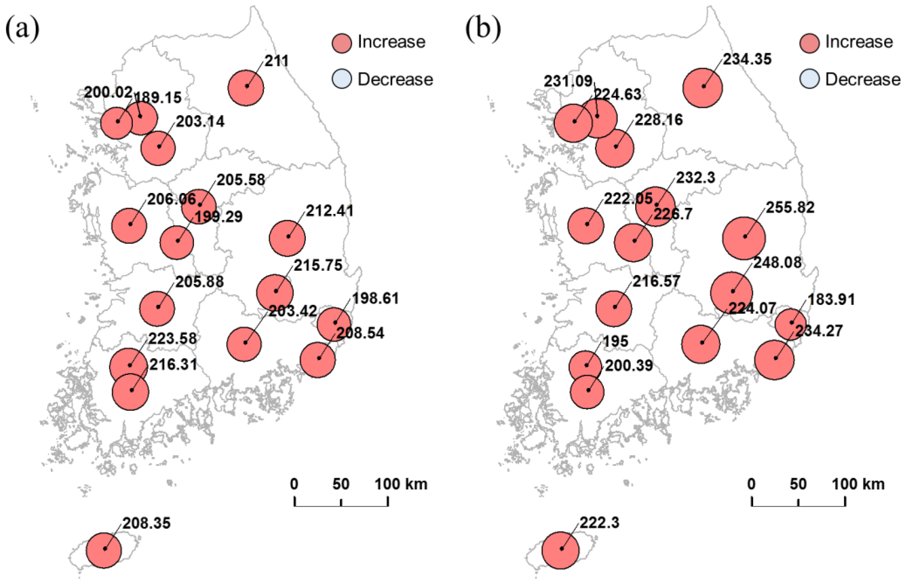
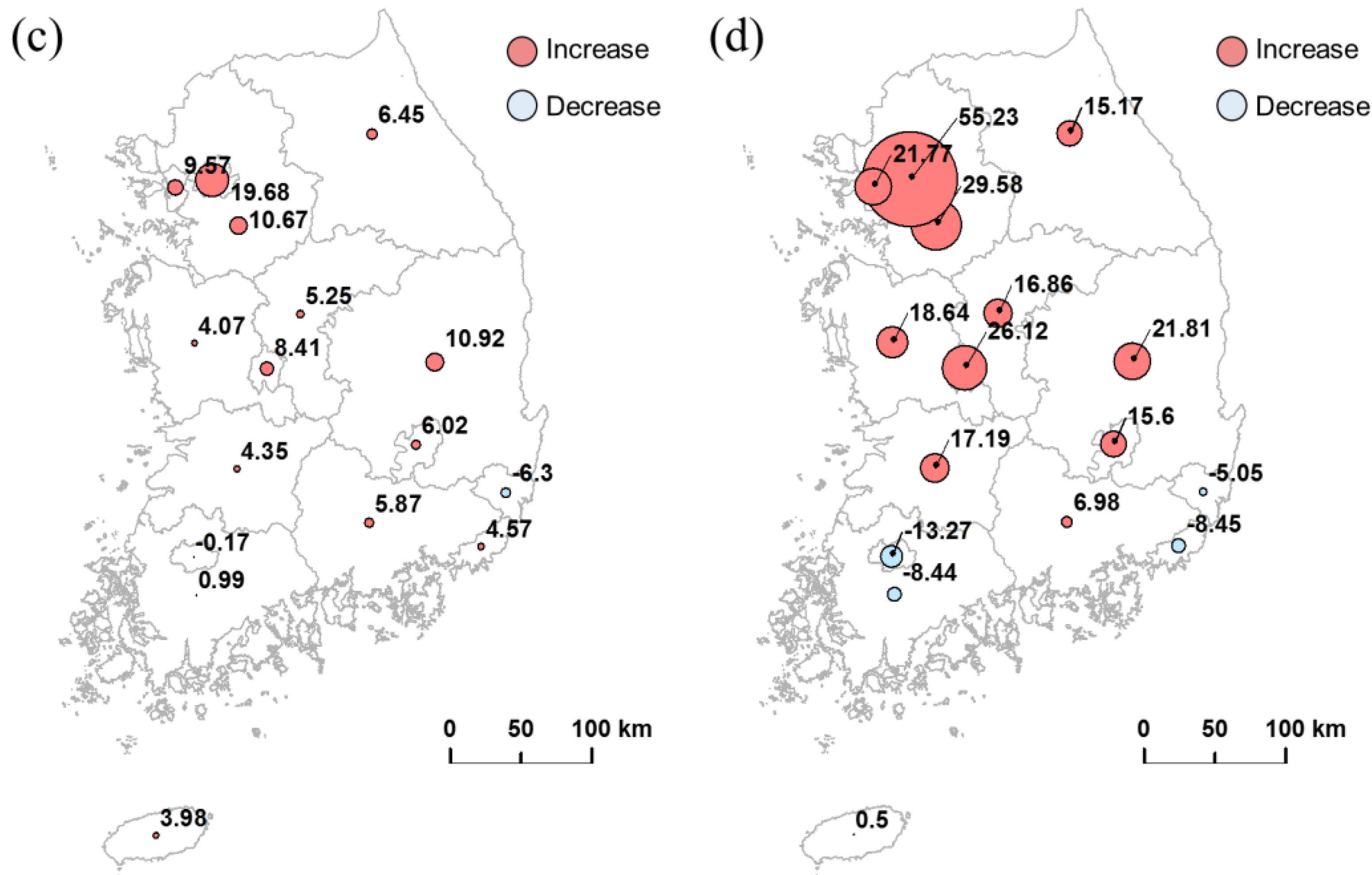
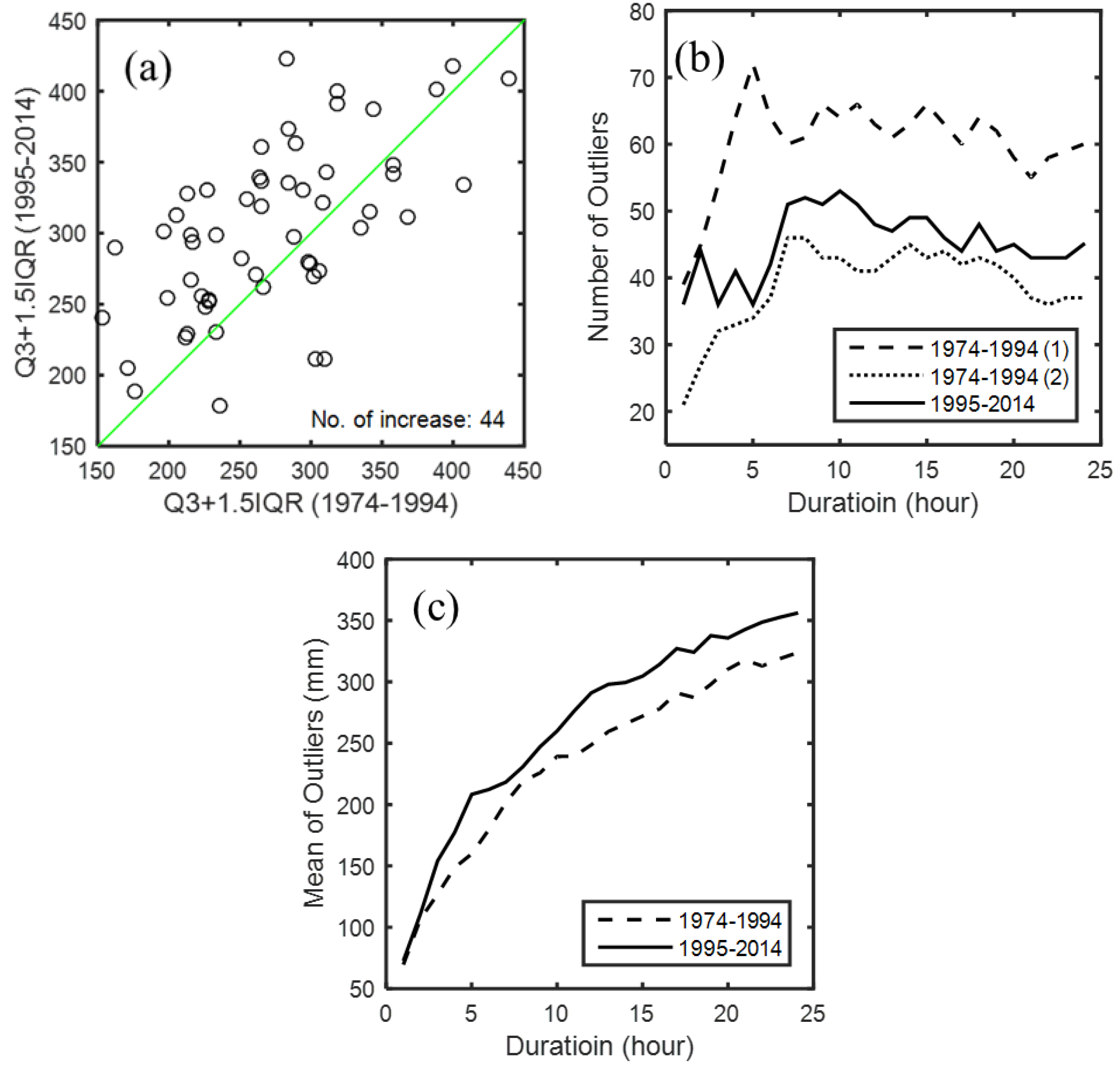
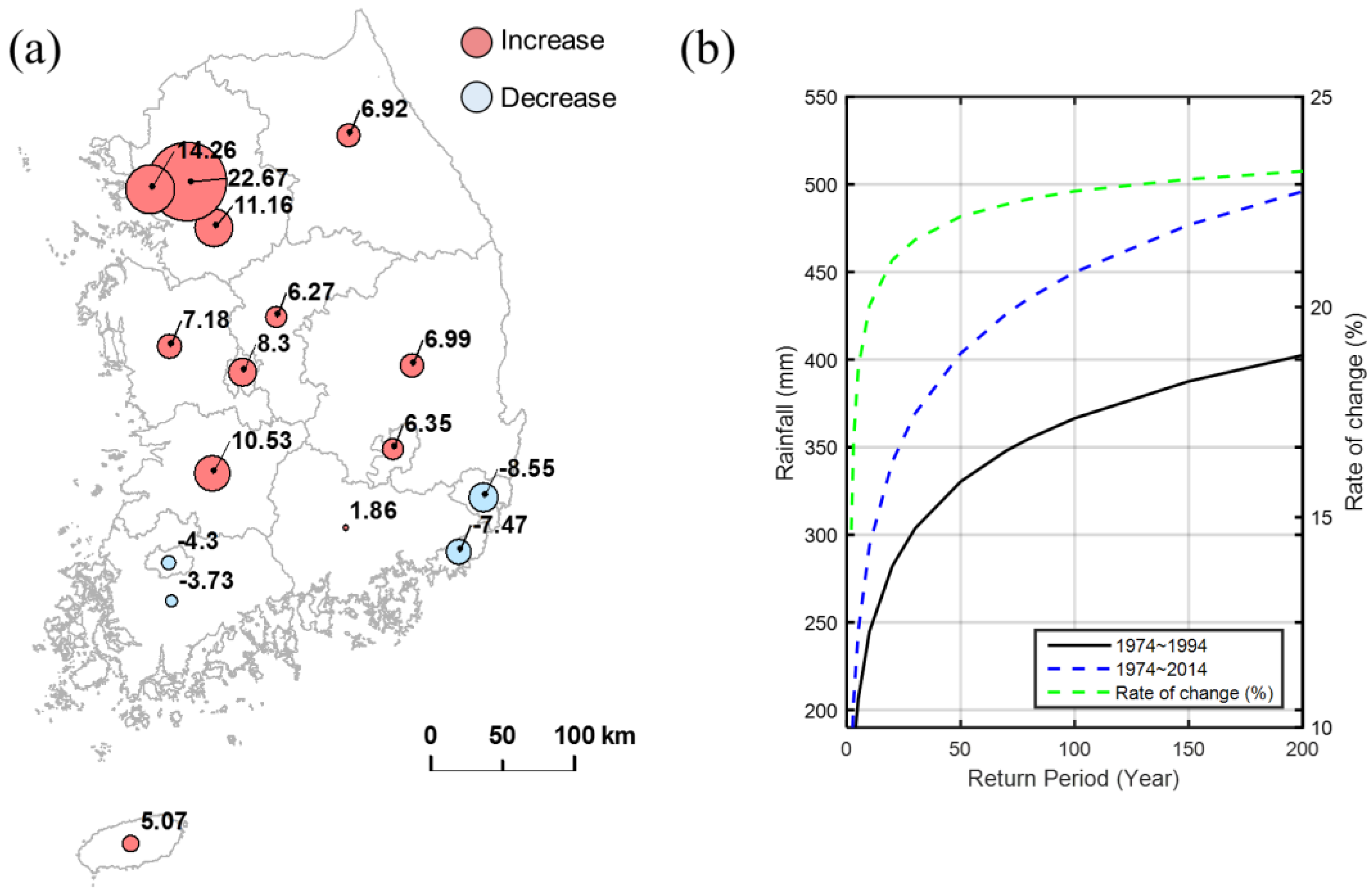
3.1. Decadal Changes in Extreme Rainfall in South Korea

The results show that the number of severe or very severe storms has increased over last two decades but the volumes showed different behavior. Figure 2 shows the changes in extreme rainfall events over last two decades (1995–2014) compared to the previous decades (1974–1994). The number of severe storms (>2 in) and very severe storms (>4 in) both doubled over last two decades. Interestingly, these changes in the number of extreme rainfalls were consistent throughout the whole country, as shown in Figure 2a,b. In contrast, Figure 2c,d shows the changes in the storm volumes of the 90th and 99th percentiles, respectively. The results show that the 90th percentile volume of rainfall events (severe storms) was increased up to 20% in Seoul (Station 108), whereas the 99th percentile volume of rainfall event was increased up to 55% in Seoul over last two decades. On the other hand, the changes differed according to the location. In particular, the southern part shows a small increase or even a decrease.
Interestingly, the frequency of extreme rainfall events increased consistently throughout the country over the last two decades but rainfall volume was not evenly changing. The results in Figure 3 strengthen this finding by showing the changes in the 24-h rainfall with a 100-year return period. As shown in Figure 3a, the rate of changes in the 24-h rainfall was up to 23% in Seoul (Station 108) but it is as low as −9% in Ulsan (Station 152). The variation of the changes in the estimated probable rainfall amount was similar to that of percentiles. The northern part of the country showed an increase in the 24-h rainfall but a decrease in the southern part.
Figure 4 shows boxplots of the 60 precipitation stations during 1974–1994 (Figure 4a) and also during 1995–2014 (Figure 4b). The outliers were defined as an observation point greater than the 1.5 interquartile range above the third quartile or lower than the 1.5 interquartile range below the first quartile. The thresholds, beyond which the outliers are defined, are presented as the grey solid line in Figure 4a and the black solid line in Figure 4b. The result shows that the number of outliers over the last two decades (1995–2014) decreased from 60 to 45 (12.5% compared to the previous two decades (1974–1994). In contrast, the global mean value of outliers was increased to 355.86 mm from 323.46 mm (10%). On the other hand, the threshold that determines the outliers, itself has increased over last two decades. The black solid line is the threshold of the second period during 1995–2014, as shown in Figure 4. If this threshold is applied to the first period during 1974–1994, the number of outliers decreases.
Figure 5a shows the changes in the threshold over the last two decades for 60 rainfall gauges in South Korea with a rainfall duration of 24 h. Among the 60 gauges, 44 gauges showed an increase in the threshold, which means that mostly, the third quartile and interquartile range increased. Figure 5b shows the number of outliers depending on their durations. As shown in Figure 5, for the rainfall duration of 24 h, the number of outliers decreased from 60 during the first period (1974–1994) to 45 during the second period (1995–2014). If threshold for the second period is applied to the first period, the number of outliers decreases to 37. This means that the number of outliers has increased if the same threshold is applied for both periods. The dots in Figure 5b show that the recalculated number of outliers has decreased consistently for all rainfall durations. In addition, the result shows that the global mean value of the outliers increased for all gauges over the last two decades, as shown in Figure 5c.
Although the changes in frequency and magnitude of the extreme events are dependent on the location, the results show that the frequency and magnitude (volume) of extreme rainfall events have increased, in general, over last two decades in South Korea. A simple analysis of the number and magnitude of outliers among the annual rainfall maxima shows that the magnitude of the outliers also increased over last two decades. In addition, the threshold itself that determines the outliers was increased, which results in the outliers 20 years ago being no longer considered as outliers in recent days. Moreover, the recent 20 years have witnessed some magnitude of outliers (circled outliers in Figure 4) that have never been experienced before. The maximum outlier was observed in Gangneung (Station 105) in 2002 during Typhoon Rusa, as mentioned in the introduction, which was 870.4 mm in one day. Note that the previous maximum rainfall was recorded in 1921. This section may be divided by subheadings. It should provide a concise and precise description of the experimental results, their interpretation as well as the experimental conclusions that can be drawn.

3.2. Physical Mechanism Behind the Changes of Extreme Events

Korea Meteorological Administration (KMA) [36,37] predicted that the amount of rainfall increase would be more than 200 mm for the next 20 years and more than 300 mm after 2040. Extreme rainfall events can be caused either by convective rainfall or Typhoon typically in Korea. Especially, for the last 20 years, heavy rainfall events caused convective rainfall tend to increase. For example, these heavy rainfall events include the extreme events in Seoul with a 100-year frequency in 2010 and 2011, Busan in 2009, Gyeonggi-do and Gangwon-do in 2008, Gangwon-do in 2006, Jeonju in 2005, and Seoul in 2001. These convective rainfall events have closely related to the geographic characteristics of Korea Peninsula neighboring both the Pacific high and the Continental high. Due to this geographic location, Korea peninsula works as a narrow alley where the warm water vapor provided from the Southeastern areas in China would be the main sources for the heavy convective rainfall. In a general sense, the temperature increase would increase humidity and, eventually, the rainfall intensity at this location. In Korea, the average temperature increased by 1.8 °C during last 100 years and it is expected to increase by 1.8–4.8 °C by 2100 based on RCP scenarios from IPCC [36].
The strength of Typhoon that affected Korea Peninsula also tends to increase. This is mainly due to changes of the origin, which is moving north. Choi et al. [38] showed the origin of Typhoon with the maximum strength moved north since 1999 by comparing the origins during 1999–2013 and 1977–1998. Choi and Moon [39] analyzed the reaching latitude of typhoon for 40 years comparing the first 20 years to the later 20 years since 1975. The maximum latitude that Typhoon traveled was increased from 28° N to 34° N during last 40 years, which means Typhoon travels north further by 660 km. This is mainly due to the seawater temperature and sea level increase around Korea peninsula [40]. Typhoons are very rare in October in Korea. However, Typhoon Chaba on October 2016, which caused the loss of 10 lives in the southeastern area, was a good example of increasing number of Typhoon due to the seawater temperature increase.

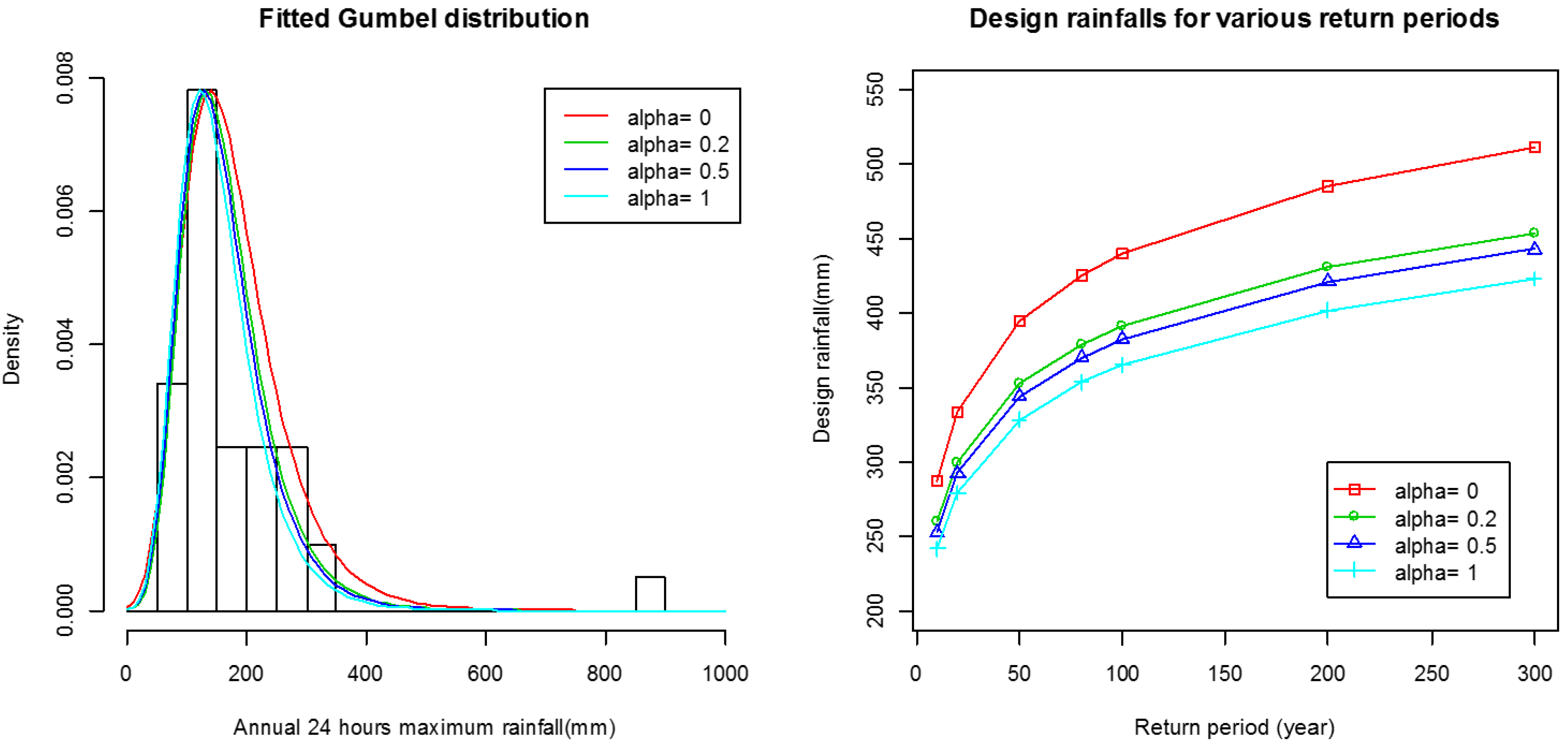
3.3. Performance of MDPDE with the Gumbel Distribution

This study considered the Gumbel distribution family as a parametric distribution family { F θ } to construct the MDPDE. The Kolmogorov–Smirnov test (K-S test) showed that the annual maxima of the 24-h duration rainfall at Gangneung follow the Gumbel distribution (GUM). Figure 6 shows the Gumbel distribution fitted to the 24-h annual maxima from 1974 to 2014 at Gangneung, where one of the extreme events was observed (870.5 mm for 24 h). In this study, we considered four cases of α = 0 ,   0.2 ,   0.5 and 1 to compare the performance of MLE and MDPDE with various   α ( 0 ,   1 ] . The different choices of α also yield similar results. As mentioned in Section 2.2, when α is equal to zero and one, MDPDE is identical to MLE and the L2 distance estimator, respectively. The MDPDE for the Gumbel distribution is summarized in Table 3, where μ ^ and σ ^ represent the estimates for location and scale parameters, respectively. As shown in Figure 6, MLE (α = 0) tends to be affected more by the extreme event (870.5 mm) than the L2 distance estimator (α = 1), which leads to more inclined distributions to the right or to the extreme event as the value of α decreases. As a result, the design rainfalls obtained with MLE (α = 0) are highest compared to other values of α regardless of the return periods. The difference between the design rainfall estimated with MLE and the L2 distance estimator was up to 17.3% depending on the recurrence interval. Consequently, the result shows that the MDPDE with α greater than zero improves the robustness, and hence, decrease the impact of an extreme event compared to MLE (α = 0).

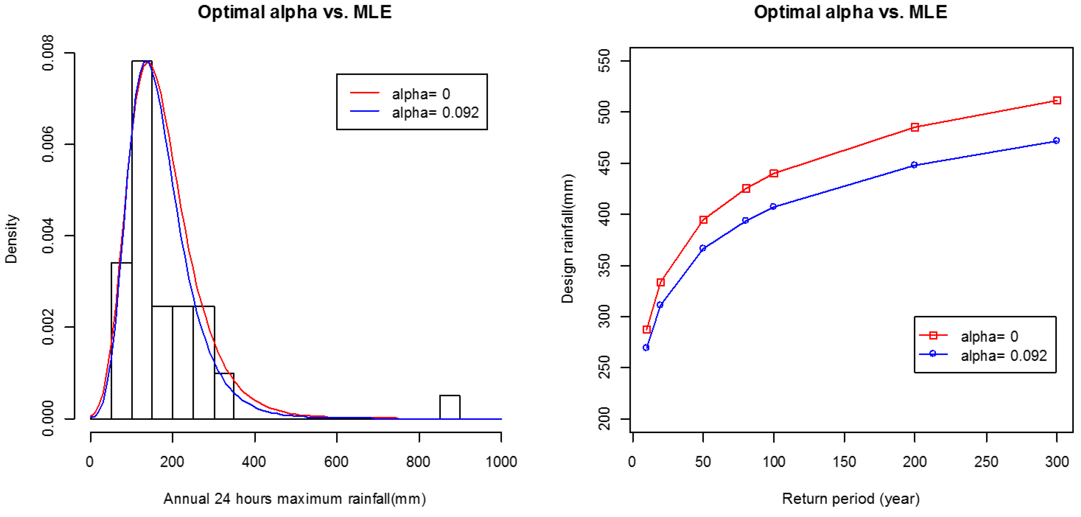
3.4. Balance between Robustness and Asymptotic Efficiency Based on the Optimal Value of α

As mentioned in Section 2.2, if the desire is to improve the robustness, adopting MDPDE with a relatively large α value can be an appropriate solution. However, as α increases, the asymptotic efficiency of MDPDE decreases because the case α = 0 corresponds to MLE, which has full asymptotic efficiency. In summary, the tuning parameter α controls the trade-off between the robustness and asymptotic efficiency. Therefore, how can the tuning parameter α be chosen in practice? In this context, we introduce a method for selecting the optimal tuning parameter, which was proposed recently by Fujisawa and Eguchi [41]. If the true distribution g is known, the optimal tuning parameter α ^ can be obtained by
α ^ = argmin α   D ( g , f θ ^ α , n ) ,
where D ( g , f ) is a divergence. As a candidate of the divergence, Fujisawa and Eguchi [41] considered the Cramer–von Mises type whose empirical version can robustly approximated by
1 n i = 1 n { i 0.5 n F θ ( x i ) } 2 ,
where x 1 , , x n are the order statistics of the observations. Combining the idea of cross validation with the above consideration, they proposed an optimal tuning parameter selection method as follows:
α ^ = argmin α 1 n i = 1 n { i 0.5 n F θ ^ α , n ( i ) ( x i ) } 2 ,
where θ ^ α , n ( i ) is the MDPDE obtained by leaving out the i th observation.
Using the 24-h annual maxima at Gangneung, an optimal value of α of 0.092 can be obtained using the optimal tuning parameter selection method. The MDPDE for the Gumbel distribution corresponding to optimal α = 0.092 is provided in Table 3. Figure 7 shows the Gumbel distribution with the optimal α value (α = 0.092) compared to MLE (α = 0). The result shows that the design rainfall estimated from MDPDE with the optimal value are greater than those from the L2 distance estimator by 11.2%–11.5% and also less than those from the MLE by 6.3%–7.7% depending on the recurrence interval from 10 to 300 years. These results indicate that MDPDE with an optimal value of α suggests an alternative way to evaluate the design rainfall with the balance between the asymptotic efficiency and robustness.
As mentioned in the introduction, the changes to the flood protection standards or design criteria cannot be achieved easily on the same timescales as those typically involved in producing scientific research. Care should be taken when implementing and applying such changes in the design standard [6]. Considering these difficulties of increasing design criteria faced with increasing frequency and magnitude of extreme events, MDPDE provides a sound and reliable alternative approach to evaluating the design rainfall.

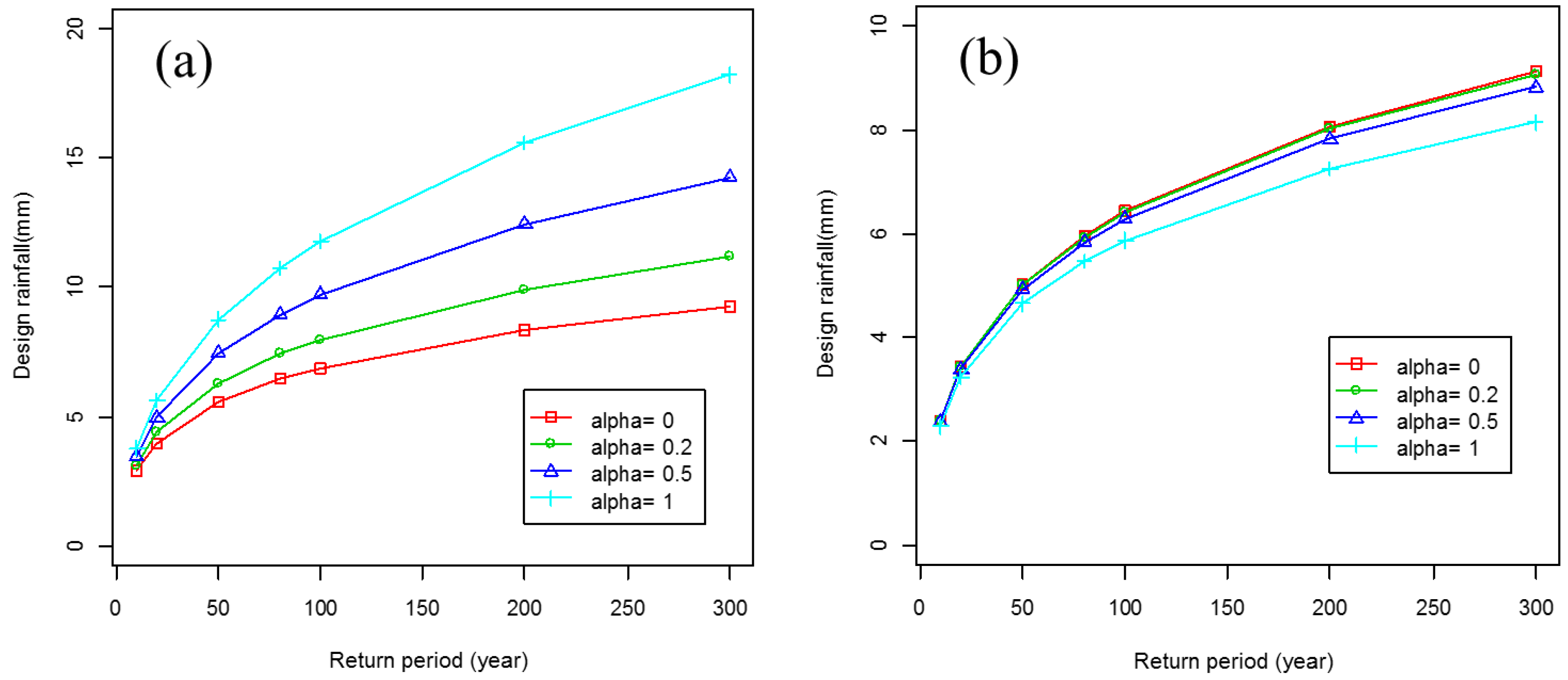
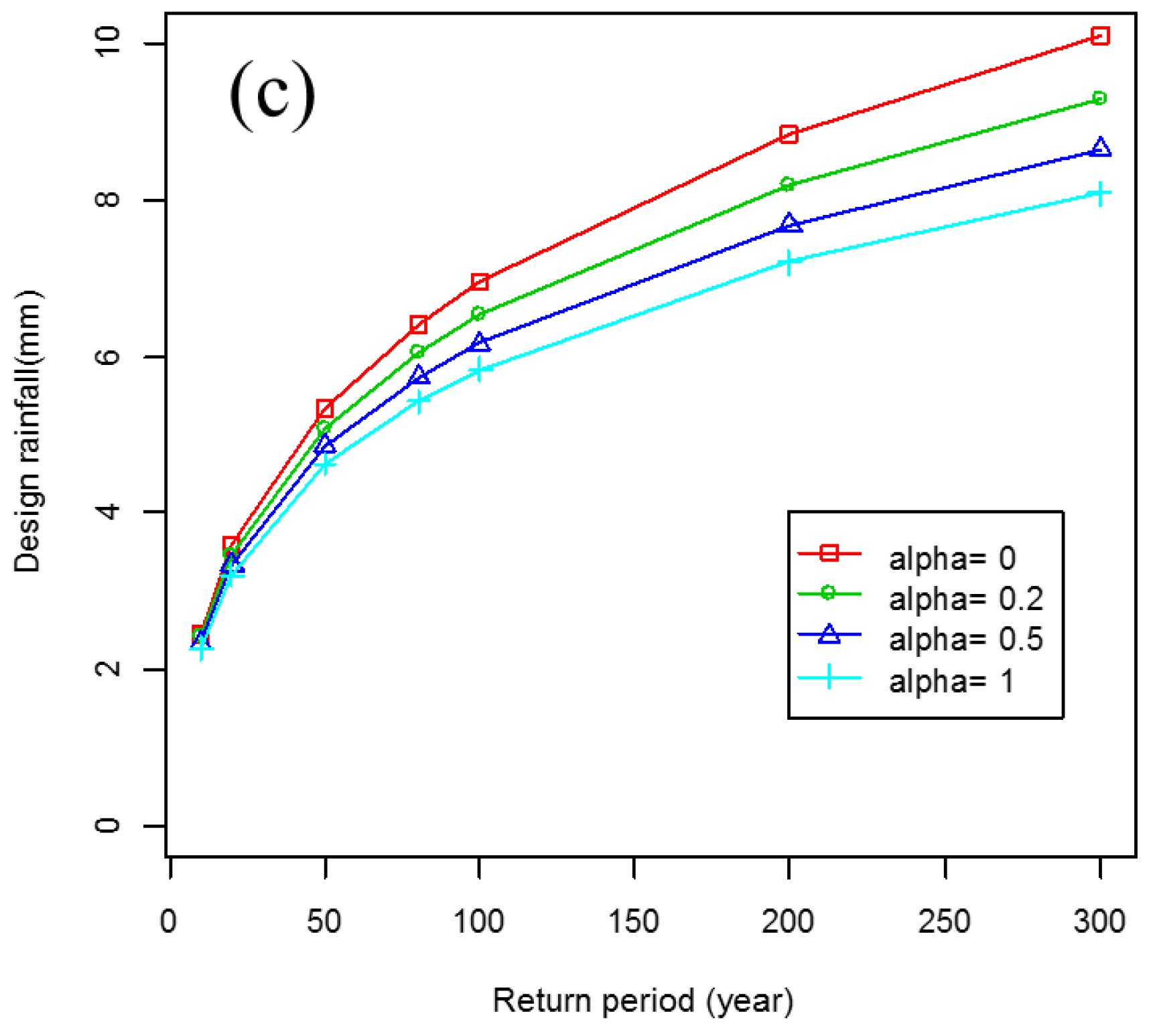
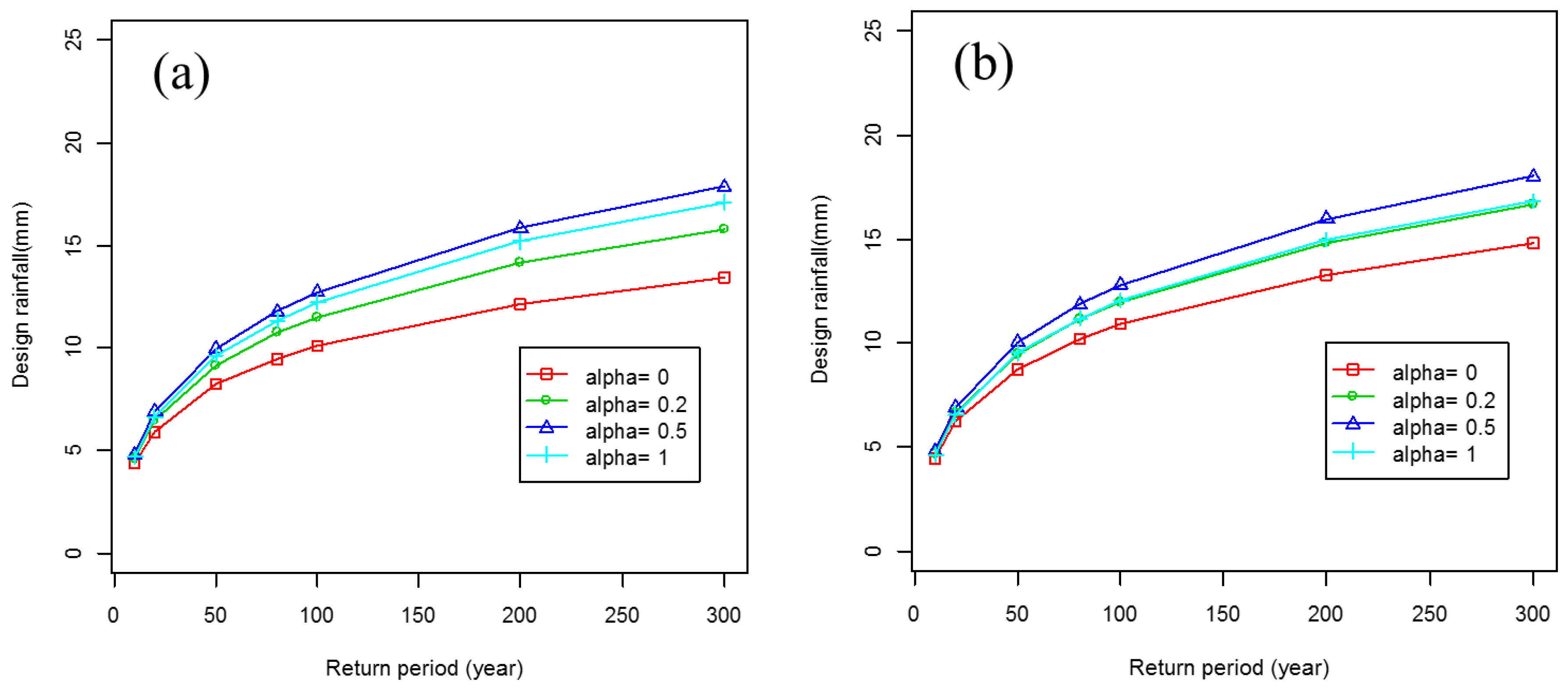
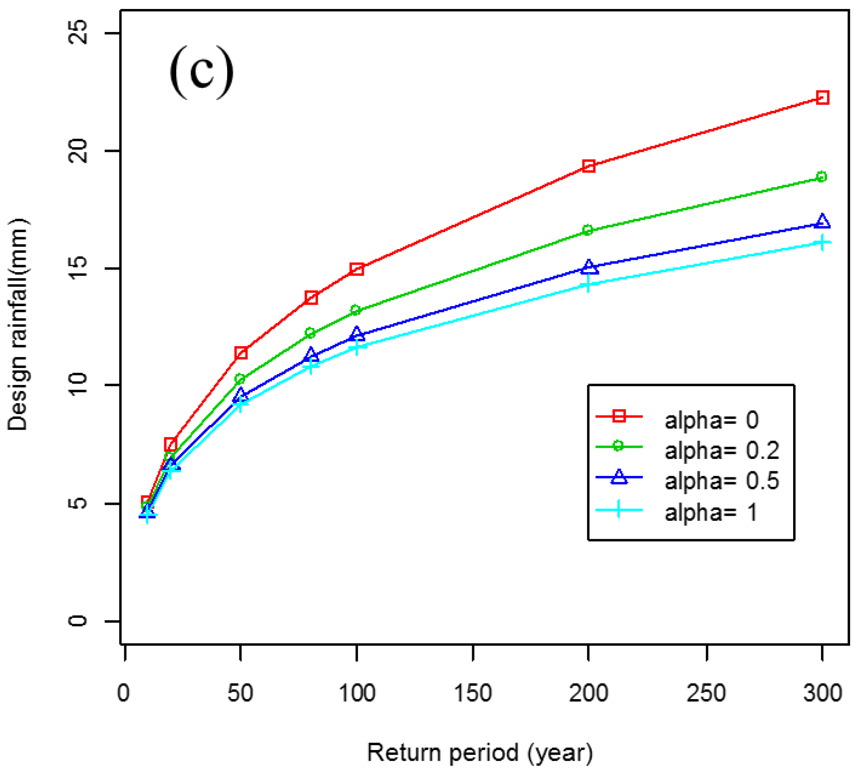
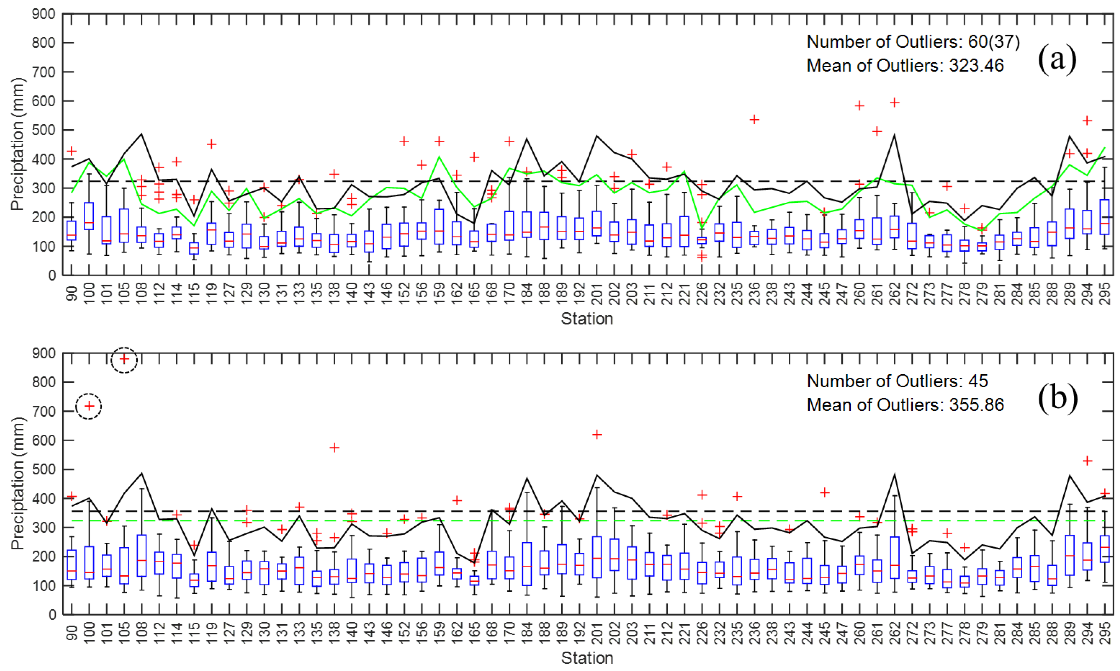
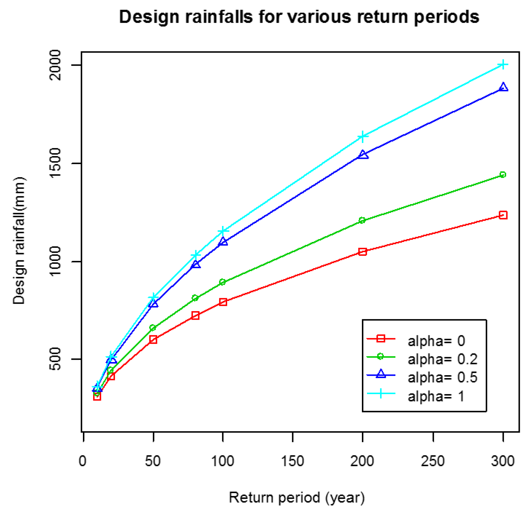
3.5. Performance of the MDPDE with GEV Depending on the Magnitude of the Extremes

In Section 3.3 and Section 3.4, the performance of MDPDE was evaluated using the Gumbel family as a parametric family { F θ } . In this section, the GEV was considered a candidate for another parametric family. However, the results were slightly different from those with GUM, where MDPDE did not reduce the design rainfall compared to MLE. The MDPDE for the GEV distribution when it was applied to the same data (Station 105) is summarized in Table 4, where μ ^ , σ ^ and ξ ^ represent the estimates for location, scale and shape parameters, respectively. Figure 8 shows the estimated design rainfall assuming the GEV. In contrast to the results in the previous section with the GUM (Figure 6b), MDPDE does not show its robust property in this case for Station 105. As the value of α increases, the estimated design rainfall also increases. The GEV has three parameters: location (μ), scale (σ) and shape parameter (ξ). The performance of MDPDE is especially related to the shape parameter (ξ), which determines the heaviness of the tail and the magnitude of the extremes. The GUM distribution is identical to GEV with ξ = 0. Therefore, the value (870.5 mm for 24 h), which was originally regarded as an outlier by the GUM, is no longer an outlier for the GEV.
For further discussion, this study evaluated the performance of MDPDE with the GEV depending on the shape parameter and also the magnitude of the extremes or outliers in this section. First, a set of random variables (50 variables) following the GEV with μ = 0, σ = 1 and ξ = 0.1 was generated (Figure 9a). The maximum value, which was originally 3.4709, was then replaced with an arbitrary larger value. Figure 9a shows the performance of the MDPDE with different values of α, which shows the opposite results compared to the Gumbel distribution with extreme events in the previous section. As the value of α increases, the estimated design rainfall also increases, which is different from the results in the previous section, where MDPDE with α > 0 showed a decrease in the design rainfall compared to MLE. These behaviors are similar to what the data of Station 105 has shown in Figure 8 for GEV. Figure 9b,c shows the results from the MDPDE after replacing the maximum value with an arbitrary larger value, 8 and 10, respectively. Compared to the case with no outlier (Figure 9a), the cases with outliers show that MDPDE shows the robust property and the same performance with the GUM case. The reason for these behaviors is that the newly added value, 8 and 10, become outliers for the GEV. As the magnitude outliers are larger (from 8 to 10), the robust property of MDPDE becomes stronger. In addition, MLE (α = 0) is more sensitive than the cases of MDPDE with α > 0, as shown in Figure 9b,c.
What if the shape factor, ξ, of the GEV is increased? ξ was increased to 0.2 with the same outliers of 8 and 10. The results showed that the increased shape parameter results in a heavier tail for GEV, which makes the previous added extremes (8 or 10) no longer outliers, and the MDPDE does not show the robust property in this case, as shown in Figure 10a,b. On the other hand, if these values (8 and 10) are replaced with a larger value of 25, the MDPDE shows a robust property. Therefore, the existence and magnitude of outliers greatly affect the performance of the MDPDE and the results also highly affected by the shape parameter in case of applying the GEV instead of the GUM distribution (ξ = 0).

4. Conclusions

The changes in extremes need to be recognized and reflect the changes in terms of improving and revising existing design and safety criteria. The existing design criteria should be evaluated under changing circumstances. On the other hand, the traditional methods, such as the MLE, can result in a sudden increase in extremes, which cannot be accepted easily by the community and result in difficulties for implementation. Often, these outliers and extremes are disregarded due to socioeconomic influences. In this regard, this study examined the changes in frequency and magnitude of extreme events in South Korea and revealed an increase in both the frequency and magnitude of extreme events over last two decades. In addition, the MDPDE was suggested as an alternative way to derive the design rainfall, which is based on the balance between the asymptotic efficiency and robustness compared to the MLE, which is relatively sensitive to extreme values. The results showed a reduced amount of estimated design rainfall by the MDPDE with the optimal tuning parameter, α, compared to the MLE. Nevertheless, care should be taken when applying the MDPDE because the behavior of the MDPDE differs according to the type of probability distribution function and heavy tails as well as the magnitude of the outliers. Overall, this study shows that the MDPDE works as an alternative estimator of design rainfall or design flood with extremes and helps us form sudden increases in design criteria in times of climate change.

Acknowledgments

This study was supported by Basic Science Research Program through the National Research Foundation of Korea (NRF) initiated by the Ministry of Science, ICT & Future Planning (NRF-2013R1A1A1058964, and NRF-2015R1C1A1A01052330).

Author Contributions

Byungsoo Kim proposed the basic idea, collected historical rainfall and flooding data in Korea. Yongwon Seo and Junshik Hwang designed the analysis procedures. The manuscript was written by Yongwon Seo with contribution from Junshik Hwang and Byungsoo Kim.

Conflicts of Interest

The authors declare no conflict of interest.

References

  1. Park, S.K.; Lee, E. Synoptic features of orographically enhanced heavy rainfall on the east coast of Korea associated with typhoon Rusa (2002). Geophys. Res. Lett. 2007, 34. [Google Scholar] [CrossRef]
  2. Lee, D.K.; Choi, S.J. Observation and numerical prediction of torrential rainfall over Korea caused by typhoon Rusa (2002). J. Geophys. Res. Atmos. 2010, 115. [Google Scholar] [CrossRef]
  3. Kim, N.W.; Won, Y.S.; Chung, I.M. The scale of typhoon Rusa. Hydrol. Earth Syst. Sci. Discuss. 2006, 3, 3147–3182. [Google Scholar] [CrossRef]
  4. Franks, S.W.; Kuczera, G. Flood frequency analysis: Evidence and implications of secular climate variability, New South Wales. Water Resour. Res. 2002. [Google Scholar] [CrossRef]
  5. Alexander, L.V.; Zhang, X.; Peterson, T.C.; Caesar, J.; Gleason, B.; Tank, A.M.G.K.; Haylock, M.; Collins, D.; Trewin, B.; Rahimzadeh, F.; et al. Global observed changes in daily climate extremes of temperature and precipitation. J. Geophys. Res. Atmos. 2006, 111. [Google Scholar] [CrossRef]
  6. Madsen, H.; Lawrence, D.; Lang, M.; Martinkova, M.; Kjeldsen, T.R. Review of trend analysis and climate change projections of extreme precipitation and floods in Europe. J. Hydrol. 2014, 519, 3634–3650. [Google Scholar] [CrossRef] [Green Version]
  7. Trenberth, K.E. Changes in precipitation with climate change. Clim. Res. 2011, 47, 123–138. [Google Scholar] [CrossRef]
  8. Intergovernmental Panel on Climate Change (IPCC). Climate Change 2014: Synthesis Report. Contribution of Working Groups I, II and III to the Fifth Assessment Report of the Intergovernmental Panel on Climate Change; IPCC: Geneva, Switzerland, 2014; p. 151.
  9. Prosdocimi, I.; Kjeldsen, T.R.; Miller, J.D. Detection and attribution of urbanization effect on flood extremes using nonstationary flood-frequency models. Water Resour. Res. 2015, 51, 4244–4262. [Google Scholar] [CrossRef] [PubMed] [Green Version]
  10. Coles, S.; Pericchi, L.R.; Sisson, S. A fully probabilistic approach to extreme rainfall modeling. J. Hydrol. 2003, 273, 35–50. [Google Scholar] [CrossRef]
  11. Strupezewski, W.G.; Kochanek, K.; Weglarczyk, S.; Singh, V.P. On robustness of large quantile estimates of log-Gumbel and log-logistic distributions to largest element of the observation series: Monte Carlo results vs. first order approximation. Stoch. Environ. Res. Risk Assess. 2005, 19, 280–291. [Google Scholar] [CrossRef]
  12. Strupczewski, W.G.; Kochanek, K.; Weglarczyk, S.; Singh, V.P. On robustness of large quantile estimates to largest elements of the observation series. Hydrol. Process. 2007, 21, 1328–1344. [Google Scholar] [CrossRef]
  13. Cunnane, C. Factors affecting choice of distribution for flood series. Hydrol. Sci. J. 1985, 30, 25–36. [Google Scholar] [CrossRef]
  14. Mutua, F.M. The use of the akaike information criterion in the identification of an optimum flood frequency model. Hydrol. Sci. J. 1994, 39, 235–244. [Google Scholar] [CrossRef]
  15. Neykov, N.; Filzmoser, P.; Dimova, R.; Neytchev, P. Robust fitting of mixtures using the trimmed likelihood estimator. Comput. Stat. Data Anal. 2007, 52, 299–308. [Google Scholar] [CrossRef]
  16. Singh, V.P. Hydrologic Frequency Modeling. In Proceedings of the International Symposium on Flood Frequency and Risk Analyses, Baton Rouge, LA, USA, 14–17 May 1986; Springer Netherlands: Dordrecht, The Netherlands, 1987; p. 645. [Google Scholar]
  17. Smith, R.L. Extreme value theory based on the r largest annual events. J. Hydrol. 1986, 86, 27–43. [Google Scholar] [CrossRef]
  18. Strupczewski, W.G.; Kochanek, K.; Singh, V.P. On the informative value of the largest sample element of log-gumbel distribution. Acta Geophys. 2007, 55, 652–678. [Google Scholar] [CrossRef]
  19. Basu, A.; Harris, I.R.; Hjort, N.L.; Jones, M.C. Robust and efficient estimation by minimising a density power divergence. Biometrika 1998, 85, 549–559. [Google Scholar] [CrossRef]
  20. Beran, R. Minimum hellinger distance estimates for parametric models. Ann. Stat. 1977, 5, 445–463. [Google Scholar] [CrossRef]
  21. Tamura, R.N.; Boos, D.D. Minimum hellinger distance estimation for multivariate location and covariance. J. Am. Stat. Assoc. 1986, 81, 223–229. [Google Scholar] [CrossRef]
  22. Simpson, D.G. Minimum hellinger distance estimation for the analysis of count data. J. Am. Stat. Assoc. 1987, 82, 802–807. [Google Scholar] [CrossRef]
  23. Basu, A.; Lindsay, B. Minimum disparity estimation for continuous models: Efficiency, distributions and robustness. Ann. Inst. Stat. Math. 1994, 46, 683–705. [Google Scholar] [CrossRef]
  24. Cao, R.; Cuevas, A.; Fraiman, R. Minimum distance density-based estimation. Comput. Stat. Data Anal. 1995, 20, 611–631. [Google Scholar] [CrossRef]
  25. Mihoko, M.; Eguchi, S. Robust blind source separation by beta divergence. Neural Comput. 2002, 14, 1859–1886. [Google Scholar] [CrossRef] [PubMed]
  26. Lee, S.; Song, J. Minimum density power divergence estimator for garch models. Test 2009, 18, 316–341. [Google Scholar] [CrossRef]
  27. Kim, B.; Lee, S. Robust estimation for the covariance matrix of multivariate time series based on normal mixtures. Comput. Stat. Data Anal. 2013, 57, 125–140. [Google Scholar] [CrossRef]
  28. Karl, T.R.; Knight, R.W.; Easterling, D.R.; Quayle, R.G. Indices of climate change for the United States. Bull. Am. Meteorol. Soc. 1996, 77, 279–292. [Google Scholar] [CrossRef]
  29. Groisman, P.Y.; Karl, T.R.; Easterling, D.R.; Knight, R.W.; Jamason, P.F.; Hennessy, K.J.; Suppiah, R.; Page, C.M.; Wibig, J.; Fortuniak, K.; et al. Changes in the probability of heavy precipitation: Important indicators of climatic change. Clim. Chang. 1999, 42, 243–283. [Google Scholar] [CrossRef]
  30. Kunkel, K.E.; Andsager, K.; Easterling, D.R. Long-term trends in extreme precipitation events over the conterminous United States and Canada. J. Clim. 1999, 12, 2515–2527. [Google Scholar] [CrossRef]
  31. Groisman, P.Y.; Knight, R.W.; Karl, T.R. Heavy precipitation and high streamflow in the contiguous United States: Trends in the twentieth century. Bull. Am. Meteorol. Soc. 2001, 82, 219–246. [Google Scholar] [CrossRef]
  32. Chu, P.S.; Chen, Y.R.; Schroeder, T.A. Changes in precipitation extremes in the Hawaiian Islands in a warming climate. J. Clim. 2010, 23, 4881–4900. [Google Scholar] [CrossRef]
  33. Spierre, S.G.; Wake, C. Trends in Extreme Precipitation Events for the Northeastern United States 1948–2007; University of New Hampshire: Durham, NH, USA, 2010. [Google Scholar]
  34. Korea Meteorological Administration (KMA). Open Portal for Meteorological Data in South Korea. Available online: https://data.kma.go.kr/cmmn/main.do (accessed on 10 September 2016).
  35. Yen, B.C.; Tung, Y.-K.; American Society of Civil Engineers. Subcommittee on Uncertainty and Reliability Analysis in Design of Hydraulic Structures. In Reliability and Uncertainty Analyses in Hydraulic Design: A Report; American Society of Civil Engineers: New York, NY, USA, 1993; p. 291. [Google Scholar]
  36. Korea Meteorological Administration (KMA). Fact Book of Climate Change in Korea; Korea Meteorological Administration: Seoul, Korea, 2011; p. 117.
  37. Korea Meteorological Administration (KMA). Learning from Recent Events in 20 Years: Top 10 Severe Rainfall Events; Korea Meteorological Administration: Seoul, Korea, 2012; p. 48.
  38. Choi, K.-S.; Park, K.-J.; Kim, J.-Y.; Kim, B.-J. Synoptic analysis on the trend of northward movement of tropical cyclone with maximum intensity. J. Korean Earth Sci. Soc. 2015, 36, 171–180. [Google Scholar] [CrossRef]
  39. Choi, K.S.; Moon, I.J. Changes in tropical cyclone activity that has affected Korea since 1999. Nat. Hazards 2012, 62, 971–989. [Google Scholar] [CrossRef]
  40. Oh, S.M.; Moon, I.J. Typhoon and storm surge intensity changes in a warming climate around the Korean peninsula. Nat. Hazards 2013, 66, 1405–1429. [Google Scholar] [CrossRef]
  41. Fujisawa, H.; Eguchi, S. Robust estimation in the normal mixture model. J. Stat. Plan. Inference 2006, 136, 3989–4011. [Google Scholar] [CrossRef]
Figure 1. Sixteen (a) Provinces in South Korea and (b) 60 rainfall gauges used in this study.
Water 09 00081 g001
Figure 2. Changes in extreme rainfall: (a) percent changes in number of events greater than 50.8 mm (2 in); (b) percent changes in number of events greater than 101.6 mm (4 in); (c) percent changes in volume of events greater than the 90th percentile; and (d) percent changes in volume of events greater than the 99th percentile.
Water 09 00081 g002aWater 09 00081 g002b
Figure 3. (a) Changes in the volume of 24-h rainfall with a 100-year return period; and (b) changes in the design rainfall for Seoul (Station 108) depending on various return periods.
Water 09 00081 g003
Figure 4. Boxplots for the annual maxima during: (a) 1974–1994; and (b) 1995–2014 for the 24-h duration; the grey dash shows the mean of the outliers during 1974–1994.
Water 09 00081 g004
Figure 5. (a) Changes in the thresholds that determine the outliers for the annual maxima of 60 stations with a rainfall duration of 24 h; (b) number of outliers during 1974–1994 and 1995–2014; and (c) mean of the outliers for each period depending on the rainfall durations.
Water 09 00081 g005
Figure 6. Gumbel distribution fitted to the 24-h annual maxima at Gangneung (Station 105) and design rainfall depending on the return periods.
Water 09 00081 g006
Figure 7. Gumbel distribution with the optimal tuning parameter (α = 0.092) and the corresponding design rainfall depending on the return periods.
Water 09 00081 g007
Figure 8. Estimated design rainfall from the GEV fitted to 24-h annual maxima at Gangneung (Station 105).
Water 09 00081 g008
Figure 9. (a) GEV (0, 1, 0.1) with no outlier; (b) replacing the maximum with an outlier of 8; and (c) with an outlier of 10.
Water 09 00081 g009aWater 09 00081 g009b
Figure 10. (a) GEV (0, 1, 0.2) replacing maximum with an outlier of 8; (b) with an outlier of 10; and (c) with outlier of 25.
Water 09 00081 g010aWater 09 00081 g010b
Table 1. Definition of heavy and very heavy rainfall used in this study.
MethodsDescription
Actual rainfall amountsHeavy rainfall: an event with precipitation above 50.8 mm (2 in)
Very heavy rainfall: an event with precipitation above 101.6 mm (4 in)
Specific thresholdsHeavy rainfall: an event with precipitation above 90th percentiles
Very heavy rainfall: an event with precipitation above 99th percentiles
Return periods Heavy rainfall event: an event with 24-h precipitation above the 20 year return period
Very heavy rainfall: an event with 24-h precipitation above the 100 year return period
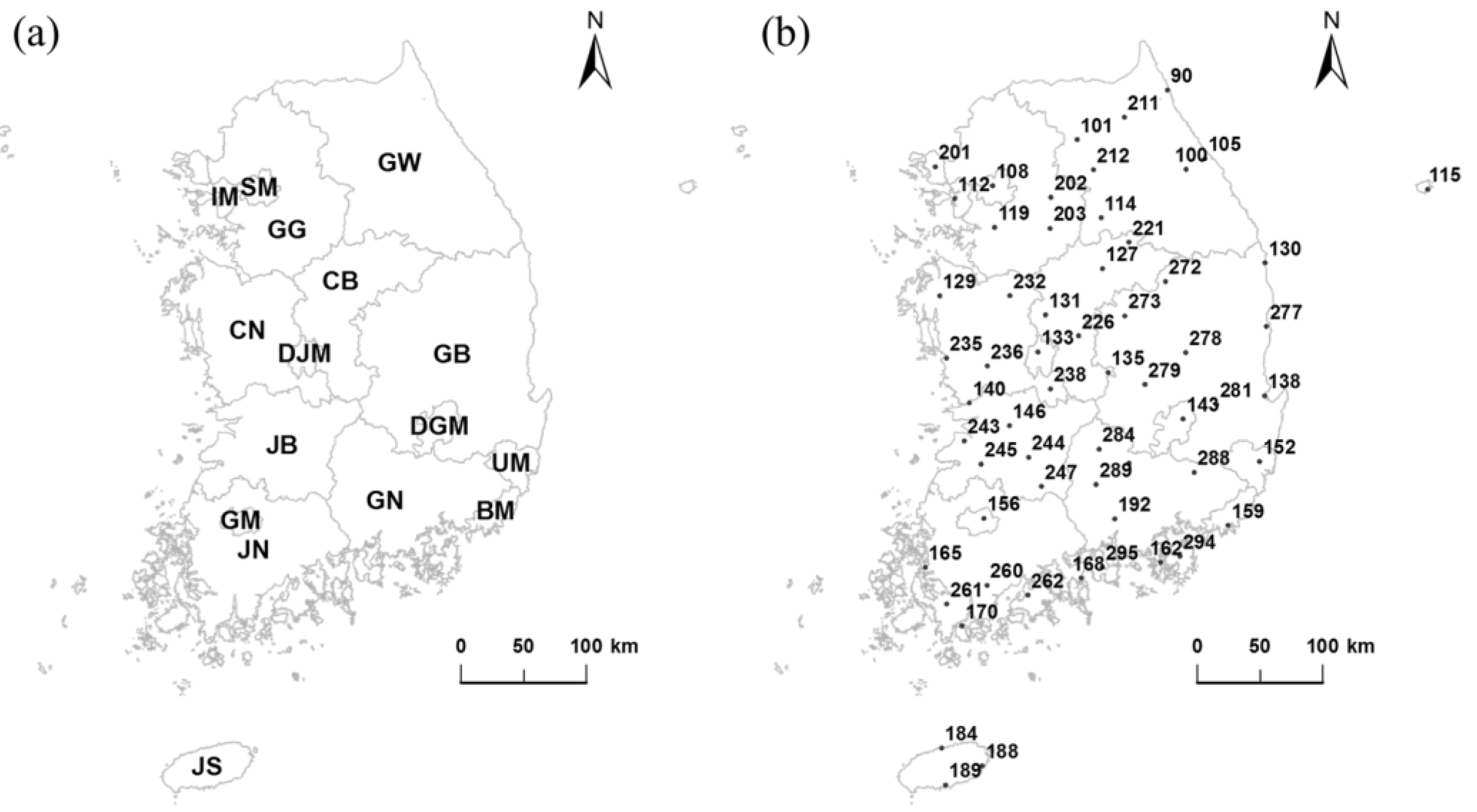
Table 2. Provinces in South Korea and rain gauges.
No.ProvinceAbbreviationRain Gauges
1Seoul Metropolitan CitySM108
2Incheon Metropolitan CityIM112
3Gyeonggi-doGG119, 201, 202, 203
4Gangwon-doGW90, 100, 101, 105, 114, 211, 212
5Chungcheongbuk-doCB127, 131, 226
6Chungcheongnam-doCN129, 135, 140, 232, 235, 236
7Daejeon Metropolitan CityDJM133
8Gyeongsangbuk-doGB115, 130, 138, 272, 273, 277, 279, 281
9Gyeongsangnam-doGN162, 192, 284, 288, 289, 295
10Daegu Metropolitan CityDGM143
11Ulsan Metropolitan CityUM152
12Busan Metropolitan CityBM159
13Jeolabuk-doJB146, 243, 244, 245, 247
14Jeolanam-doJN165, 170, 260, 261, 262
15Gwangju Metropolitan CityGM156
16Jeju IslandJS184, 188, 189
Table 3. MDPDE for the Gumbel distribution according to α .
α 00.20.510.092
μ ^ 139.413132.468128.227122.340135.257
σ ^ 65.36056.35455.28652.81559.122
Table 4. MDPDE for the GEV distribution according to α .
α 00.20.51
μ ^ 126.380126.453126.705126.461
σ ^ 49.74751.75954.61556.341
ξ ^ 0.4040.4380.4970.506

