Experimental and Numerical Analysis of a Water Emptying Pipeline Using Different Air Valves

Abstract

The emptying procedure is a common operation that engineers have to face in pipelines. This generates subatmospheric pressure caused by the expansion of air pockets, which can produce the collapse of the system depending on the conditions of the installation. To avoid this problem, engineers have to install air valves in pipelines. However, if air valves are not adequately designed, then the risk in pipelines continues. In this research, a mathematical model is developed to simulate an emptying process in pipelines that can be used for planning this type of operation. The one-dimensional proposed model analyzes the water phase propagation by a new rigid model and the air pockets effect using thermodynamic formulations. The proposed model is validated through measurements of the air pocket absolute pressure, the water velocity and the length of the emptying columns in an experimental facility. Results show that the proposed model can accurately predict the hydraulic characteristic variables.

1. Introduction

The emptying procedure in a pipeline generates hydraulic events that can cause problems if air valves are not well sized. In practical applications, engineers follow typical recommendations from the American Water Works Association (AWWA) [1] or manufacturers about sizing and location of air valves along a pipeline in order to avoid subatmospheric pressure that can cause the collapse of the system. It is recommended in a pipeline that the air volume admitted by air valves should be the same as the water volume drained [2]. Consequently, air valves should work in subsonic flow conditions. Air valves should be located at high points, in long horizontal pipe branches, long descents, long ascents, at the decrease in an up-slope and increase in a down-slope of a pipeline, and on the discharge side of deep well pumps and at vertical turbines/pumps [1]. An inappropriate selection of the air valve size and location produces not only subatmospheric pressure but also a slow drainage of the system.

Presently, there are only few studies related to the emptying process in the literature, but they are not focused on practical applications because they do not consider a pipeline with an irregular profile [3] and air valves [4,5].

The analysis of an emptying process is not trivial because it requires the study of a two-phase flow [6,7,8,9]. This problem can be studied using one (1D) [10,11], two (2D) [12] or three-dimensional (3D) [13] models. The water phase in the 1D model can be analyzed considering two types of models [14]: (i) elastic models [15,16], which consider the elasticity of the pipe and the water; or (ii) rigid models [17], which ignore the elasticity of them. Normally, elastic models are solved by using the method of characteristics [18,19] and rigid models by using the numerical solutions of ordinary differential equations [3,11,17,20]. In pressurized systems, the air effect can be analyzed as a single-phase flow, where the absolute pressure of the air pocket is computed between two water columns [10,11,21]. Regarding the analysis of 2D and 3D CFD modeling of air-water interface in closed pipes, they are still unyielding in the application of pipeline draining because length and time scales are not appropriate.

This research develops a general 1D mathematical model that can be used for analyzing the behaviour of the main hydraulic variables during the emptying process in a pipeline with an irregular profile and with several air valves installed along it based on formulations of previous works [3,10,11,17,20,22,23]. The proposed model can give important information in real systems about: (i) the risk of collapse of pipeline installations, by checking in a pipe manufacturer characteristics if the stiffness class is appropriate to support the subatmospheric pressure reached during the hydraulic event depending on the type of soil in natural conditions, the type of backfill and the cover depth; (ii) the appropriate selection of the air valve during the emptying process; (iii) the size and the maneuver time of the drain valves; and (iv) the estimation of the drainage time of a pipeline.

2. Mathematical Model

Figure 1 shows a typical configuration of an irregular profile in a pipeline which consists of n entrapped air pockets, d air valves, p pipes, and o drain valves located at low points for draining the system, D being the internal pipe diameter (m); A being the cross section area of the pipe (${\mathrm{m}}^2$); f being the Darcy–Weisbach friction factor; and g being the gravity acceleration ($\mathrm{m}/{\mathrm{s}}^2$). $L_j$ ($j=1,2,...,p$) is the total length of each pipe, $A{V}_m$ ($m=1,2,...,d$) are the air valves, and $K_s$ ($s=1,2,...,o$) represents the flow factor for each drain valve. The emptying process starts when the drain valves are opened, thus air valves start to admit air into the pipeline. After that, the air pocket i will begin to expand generating subatmospheric pressure. At the same time, the drainage of the water column starts until the entire pipeline is completely emptied. Figure 1 gives the evolution at time t, the length of the emptying column $L_{e,j}$ ($j=1,2,...,p$), the absolute pressure of the air pocket $p_i^{*}$ ($i=1,2,...,n$), and the water velocity $v_{e,j}$ ($j=1,2,...,p$). The expansion of the air pocket i can be computed as $x_i=L_j-L_{e,j}+L_{j+1}-L_{e,j+1}$.

The one-dimensional (1D) proposed model has the following assumptions: (1) water column has been modeled by the rigid model; (2) the Darcy–Weisbach equation was considered to evaluate friction losses; (3) the thermodynamic behaviour of the air pocket is analyzed using a polytropic model; and (4) the air–water interface is perpendicular to the pipe direction. The proposed model can be used for pipelines with small diameters and with hydraulic slopes enough to prevent downstream air intrusion where open-channel flow does not occur [20,24].

Under these hypotheses, the problem is modeled by the following set of equations.

2.1. Equations for the Water Phase

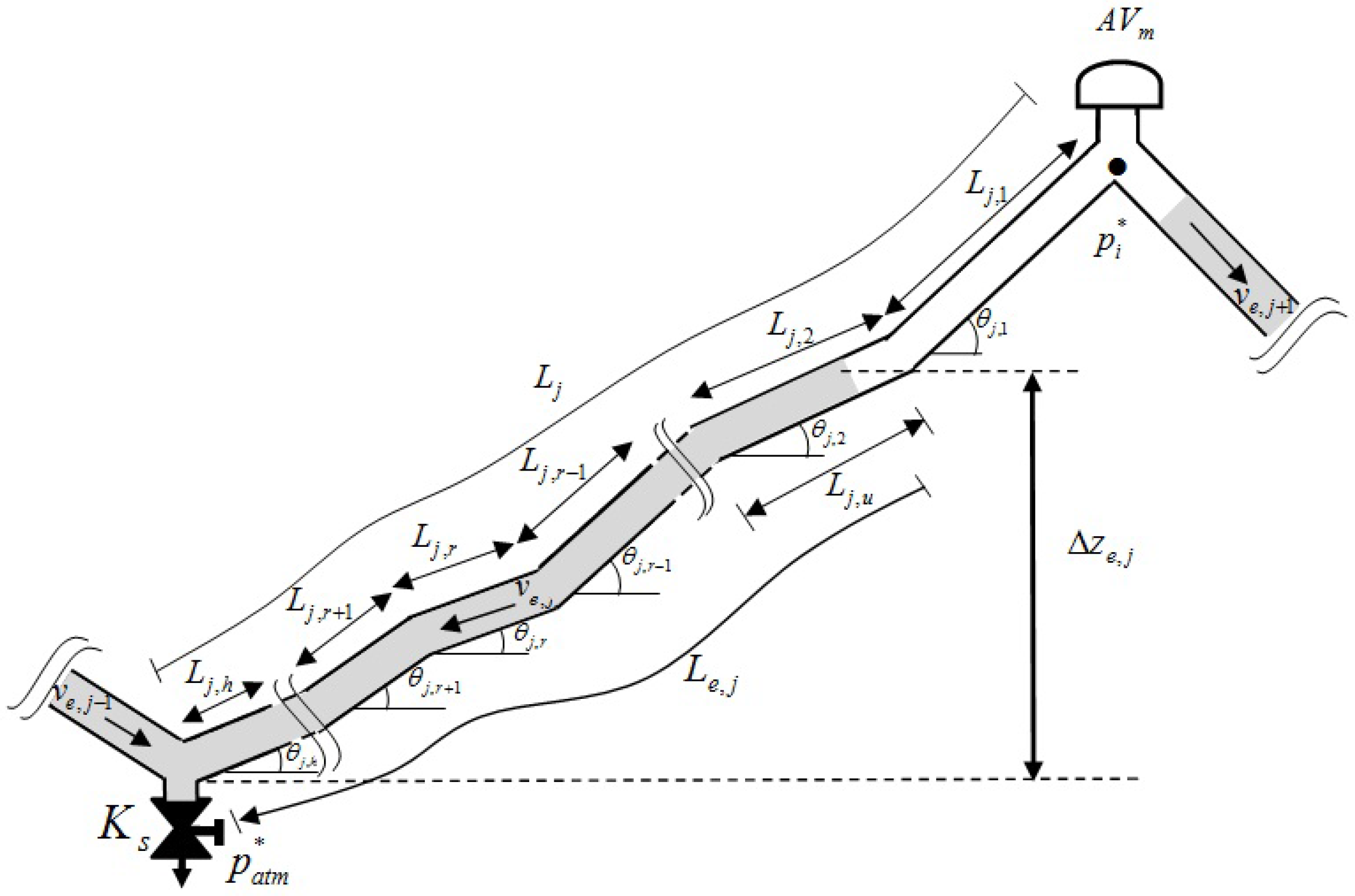
• Mass oscillation equation:
  The rigid model was used in order to compute the evolution of the water column [11,25], considering that the elasticity of the air is much higher than the elasticity of the pipe and the water [12]. Applying the rigid model to the emptying column j and considering that the drain valve s joins pipes $L_j$ and $L_{j-1}$, which is a common point in a pipeline, then:

  $$\frac{d{v}_{e,j}}{dt}=\frac{p_i^{*}-p_{atm}^{*}}{{\rho }_w{L}_{e,j}}+g\frac{\mathrm{\Delta }{z}_{e,j}}{L_{e,j}}-f_j\frac{v_{e,j}\left|v_{e,j}\right|}{2D}-\frac{g{A}^2(v_{e,j}+v_{e,j-1})|v_{e,j}+v_{e,j-1}|}{L_{e,j}{K}_s^2},$$

  (1)

  where $\mathrm{\Delta }{z}_{e,j}$ is the elevation difference (m), ${\rho }_w$ is the water density ($\mathrm{k}\mathrm{g}/{\mathrm{m}}^3$), $p_{atm}^{*}$ is the atmospheric pressure (101,325 Pa) and g is the gravity acceleration ($\mathrm{m}/{\mathrm{s}}^2$).
  The expression $h_{m,s}=Q_{w,s}^2/K_s^2$ was used to estimate the local loss of the drain valve s in Equation (1). $K_s$ is the flow factor and $Q_{w,s}$ is the water discharge.
  If the drain valve only connects pipe $L_j$, thus $v_{e,j-1}=0$.
• Air–water interface position:
  The position of the air–water interface is considered perpendicular to the pipe direction [11,18,26]. The continuity equation for the moving air-water interface j is:

  $$\frac{d{L}_{e,j}}{dt}=-v_{e,j}\left(L_{e,j}=L_{e,j,0}-{\int }_0^t{v}_{e,j}\mathrm{d}t\right),$$

  (2)

  where subscript 0 refers to the initial condition.

2.2. Equations for Air Pockets

• Continuity equation [3,17]:

  $$\frac{d{m}_{a,i}}{dt}={\rho }_{a,nc}{v}_{a,nc,m}{A}_{adm,m}$$

  (3)

  and by deriving:

  $$\frac{d{m}_{a,i}}{dt}=\frac{d\left({\rho }_{a,i}{V}_{a,i}\right)}{dt}=\frac{d{\rho }_{a,i}}{dt}{V}_{a,i}+\frac{d{V}_{a,i}}{dt}{\rho }_{a,i},$$

  (4)

  where $m_{a,i}$ is the air mass and $V_{a,i}$ is the air volume of the air pocket i.
  Due to the air pocket i located between pipes $L_j$ and $L_{j+1}$, then $V_{a,i}=(L_j-L_{e,j})A+(L_{j+1}-L_{e,j+1})A$ and $d{V}_{a,i}/dt=-(d{L}_{e,j}/dt)A-(d{L}_{e,j+1}/dt)A=A(v_{e,j}+v_{e,j+1})$, thus:

  $$\frac{d{\rho }_{a,i}}{dt}=\frac{{\rho }_{a,nc}{v}_{a,nc,m}{A}_{adm,m}-(v_{e,j+1}+v_{e,j})A{\rho }_{a,i}}{A(L_j-L_{e,j}+L_{j+1}-L_{e,j+1})},$$

  (5)

  where ${\rho }_{a,i}$ is the air density of the air pocket i, ${\rho }_{a,nc}$ is the air density in normal conditions ($1.205$ $\mathrm{k}\mathrm{g}/{\mathrm{m}}^3$), $A_{adm,m}$ is the cross section area (${\mathrm{m}}^2$) of the air valve m and $v_{a,nc,m}$ is the air velocity in normal conditions admitted by the air valve m.
• Expansion equation for the air pocket i:
  the thermodynamic behaviour of the air pocket [27] is treated by using a polytropic model [22,28]

  $$\frac{d{p}_i^{*}}{dt}=-k\frac{p_i^{*}}{V_{a,i}}\frac{d{V}_{a,i}}{dt}+\frac{p_i^{*}}{V_{a,i}}\frac{k}{{\rho }_{a,i}}\frac{d{m}_{a,i}}{dt}.$$

  (6)
  Considering the equations presented before, then:

  $$\frac{d{p}_i^{*}}{dt}=\frac{k{p}_i^{*}}{A(L_j-L_{e,j}+L_{j+1}-L_{e,j+1})}\left(\frac{{\rho }_{a,nc}{v}_{a,nc,i}{A}_{adm,m}}{{\rho }_{a,i}}-A(v_{e,j+1}+v_{e,j})\right),$$

  (7)

  where k is the polytropic coefficient: if $k=1.0$, then the process is isothermal, but, if $k=1.4$, the process is adiabatic.
  In Equations (5) and (7), if the air pocket i is only located in pipe $L_j$, then $v_{e,j+1}=0$ and $L_{j+1}=L_{e,j+1}=0$.
• Air valve characterization:
  The formulation proposed by Wylie and Streeter [23,29] was used to represent the air admission into the system for air valves. Ideally, the air valve m should be working in subsonic flow ($p_{atm}^{*}>p_i^{*}>0.528p_{atm}^{*}$), then:

  $$Q_{a,nc,m}=C_{adm,m}{A}_{adm,m}\sqrt{7p_{atm}^{*}{\rho }_{a,nc}\left[{\left(\frac{p_i^{*}}{p_{atm}^{*}}\right)}^{1.4286}-{\left(\frac{p_i^{*}}{p_{atm}^{*}}\right)}^{1.714}\right]},$$

  (8)

  where $Q_{a,nc,m}$ is the air discharge in normal conditions admitted by the air valve m and $Q_{a,nc,m}=v_{a,nc,m}{A}_{adm,m}$.

When air valves are not located in high points of the system, then the position of them should be specified. When the air–water interface reaches an air valve, then it starts to admit air inside the system.

In summary, a set of $2p+2n+d$ equations describes the whole system. Together with the corresponding boundary conditions, it can be solved for the $2p+2n+d$ unknowns $v_{e,j},L_{e,j},p_i^{*},{\rho }_{a,i},v_{a,nc,m}(j=1,2,...,p;i=1,2,...,n;m=1,2,...,d)$.

2.3. Initial and Boundary Conditions

When the pipeline is at rest, the initial conditions are described as follows: $v_{e,j}\left(0\right)=0(j=1,2,..,p)$, $L_{e,j}\left(0\right)=L_{e,j,0}(j=1,2,..,p)$, $p_i^{*}\left(0\right)=p_{i,0}^{*}(i=1,2,..,n)$, ${\rho }_{a,i}\left(0\right)={\rho }_{a,i,0}(i=1,2,..,n)$, and $v_{a,nc,m}\left(0\right)=0(i=1,2,..,d)$.

The upstream boundary condition is given by $p_i^{*}=p_{i,0}^{*}$, the downstream is given by the flow factor $K_s$ of the drain valve s, and the atmospheric pressure $p_{atm}^{*}$ due to the free discharge.

2.4. Gravity Term

Figure 2 describes the evolution of the gravity term (see Equation (1)) along the emptying column j. $L_{j,r}$ ($r=1,2,...,h$) is the length of the pipe reach r, and $L_j$ is the total pipe length j ($L_j={\sum }_{r=1}^{r=h}{L}_{j,r}$). Subscript u is used to identify the pipe reaches (1 to h) where the air–water interface is located.

The gravity term of the emptying column j is computed by:

• When the air–water interface has not arrived the last reach ($r\ne h$):

  $$\frac{\mathrm{\Delta }{z}_{e,j}}{L_{e,j}}=\frac{{\sum }_{r=u+1}^{r=h}{L}_{j,r}sin\left({\theta }_{j,r}\right)}{L_{e,j}}+(1-\frac{{\sum }_{r=u+1}^{r=h}{L}_{j,r}}{L_{e,j}})sin\left({\theta }_{j,u}\right).$$

  (9)
• When the air–water interface is located on the last reach ($r=h$):

  $$\frac{\mathrm{\Delta }{z}_{e,j}}{L_{e,j}}=sin\left({\theta }_{j,h}\right).$$

  (10)

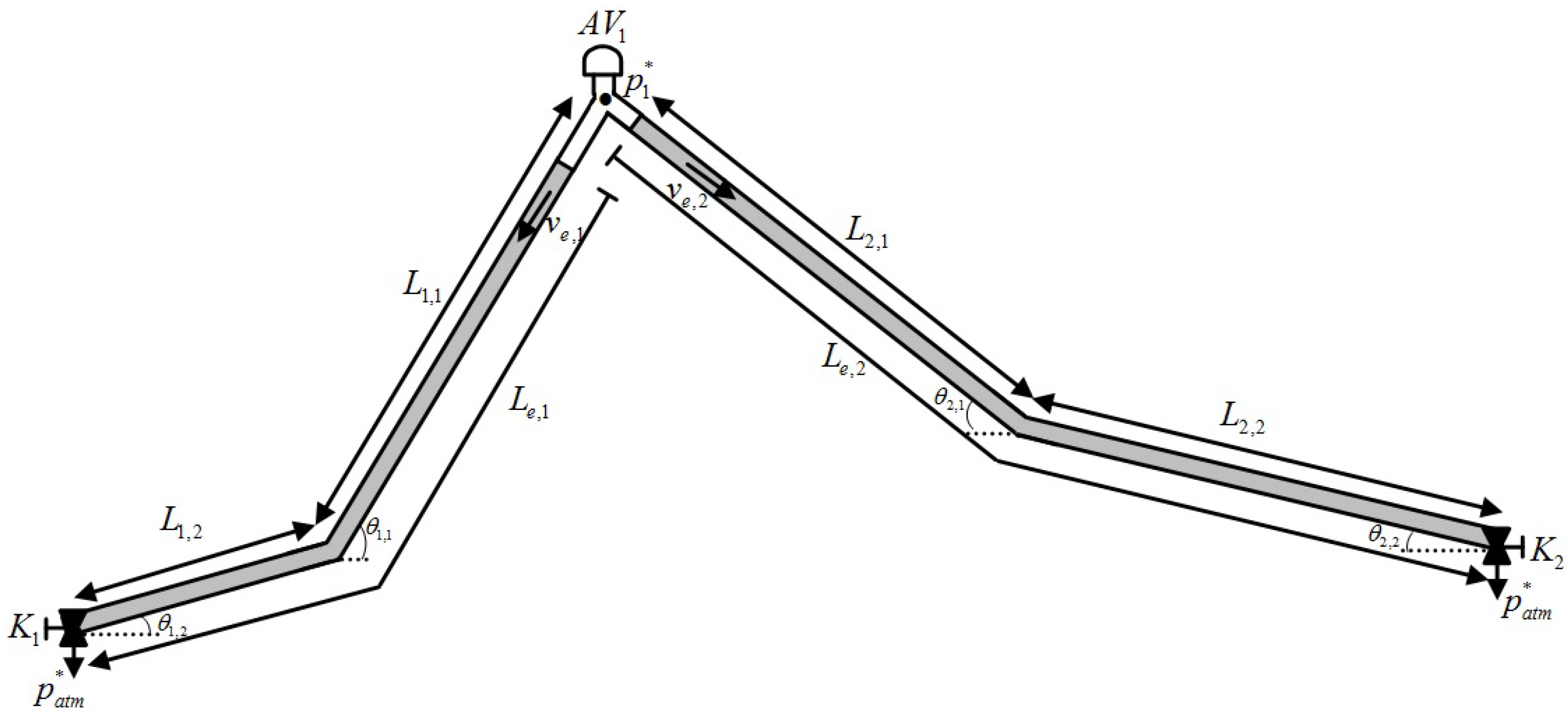
3. Application to Two Emptying Columns

Figure 3 presents a case of two emptying columns. More complex systems can be treated in the same way based on the proposed model.

The corresponding equations of the pipeline are:

• Mass oscillation equation applied to the emptying column 1

  $$\frac{d{v}_{e,1}}{dt}=\frac{p_1^{*}-p_{atm}^{*}}{{\rho }_w{L}_{e,1}}+g\frac{\mathrm{\Delta }{z}_{e,1}}{L_{e,1}}-f_1\frac{v_{e,1}\left|v_{e,1}\right|}{2D}-\frac{g{A}_1^2{v}_{e,1}\left|v_{e,1}\right|}{K_1^2{L}_{e,1}}.$$

  (11)
• Emptying column 1 position

  $$\frac{d{L}_{e,1}}{dt}=-v_{e,1}\left(L_{e,1}=L_{e,1,0}-{\int }_0^t{v}_1\mathrm{d}t\right).$$

  (12)
• Mass oscillation equation applied to the emptying column 2

  $$\frac{d{v}_{e,2}}{dt}=\frac{p_1^{*}-p_{atm}^{*}}{{\rho }_w{L}_{e,2}}+g\frac{\mathrm{\Delta }{z}_{e,2}}{L_{e,2}}-f_2\frac{v_{e,2}\left|v_{e,2}\right|}{2D}-\frac{g{A}_2^2{v}_{e,2}\left|v_{e,2}\right|}{K_2^2{L}_{e,2}}.$$

  (13)
• Emptying column 2 position

  $$\frac{d{L}_{e,2}}{dt}=-v_{e,2}\left(L_{e,2}=L_{e,2,0}-{\int }_0^t{v}_{e,2}\mathrm{d}t\right).$$

  (14)
• Evolution of the air pocket

  $$\frac{d{p}_1^{*}}{dt}=-k\frac{p_1^{*}(v_{e,1}{A}_1+v_{e,2}{A}_2)}{A_2(L_2-L_{e,2})+A_1(L_1-L_{e,1})}+\frac{p_1^{*}{\rho }_{a,nc}{v}_{a,nc,1}{A}_{adm,1}}{A_2(L_2-L_{e,2})+A_1(L_1-L_{e,1})}\frac{k}{{\rho }_{a,1}}.$$

  (15)
• Continuity equation of the air pocket

  $$\frac{d{\rho }_{a,1}}{dt}=\frac{{\rho }_{a,nc}{v}_{a,nc,1}{A}_{adm,1}-(v_{e,1}{A}_1+v_{e,2}{A}_2){\rho }_{a,1}}{A_2(L_2-L_{e,2})+A_1(L_1-L_{e,1})}.$$

  (16)
• Air valve characterization

  $$Q_{a,nc,1}=C_{adm,1}{A}_{adm,1}\sqrt{7p_{atm}^{*}{\rho }_{a,nc}\left[{\left(\frac{p_1^{*}}{p_{atm}^{*}}\right)}^{1.4286}-{\left(\frac{p_1^{*}}{p_{atm}^{*}}\right)}^{1.714}\right]}.$$

  (17)

This set of seven differential-algebraic equations (Equations (11) to (17)), together with the initial condition given by $v_{e,1}\left(0\right)=0$, $L_{e,1}\left(0\right)=L_{e,1,0}$, $v_{e,2}\left(0\right)=0$, $L_{e,2}\left(0\right)=L_{e,2,0}$, $p_{1,0}^{*}=p_{atm}^{*}=$ 101,325 Pa, ${\rho }_{a,1,0}={\rho }_{a,nc}=1.205$ $\mathrm{k}\mathrm{g}/{\mathrm{m}}^3$ and $Q_{a,nc,1}\left(0\right)=0$, allow for describing the whole problem. The Simulink Library in Matlab ( The MathWorks, Inc., Natick, MA, USA) was used in order to compute the seven unknown functions: $v_{e,1}$, $L_{e,1}$, $v_{e,2}$, $L_{e,2}$, $p_1^{*}$, ${\rho }_{a,1}$ and $Q_{a,nc,1}$.

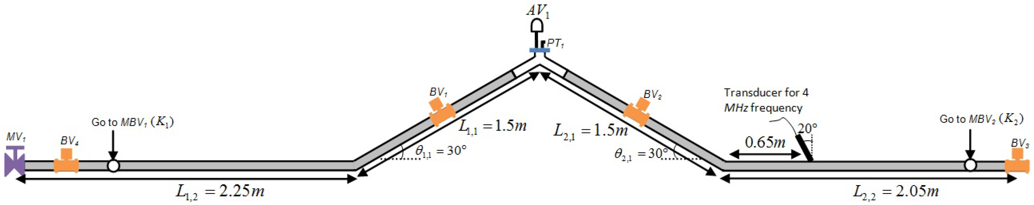
3.1. Experimental Model

In order to study the emptying process in a pipeline, an experimental facility was developed (see Figure 4) at the Civil Engineering, Research and Innovation for Sustainability (CEris) Center, in the Hydraulic Lab of Instituto Superior Técnico (IST), University of Lisbon, Portugal. The experimental facility consisted of a set of transparent PVC pipes with $7.3$ m length and nominal diameter of 63 mm $\left(DN63\right)$. An air valve ($A{V}_1$) was installed at the highest point of the pipeline with a pressure transducer $\left(P{T}_1\right)$ to measure the absolute pressure. The air valves $S050$ and $D040$ (manufacturer A.R.I.) and different air pocket sizes were tested for showing the effect on the hydraulic behaviour. There were four ball valves ($B{V}_s)$. $B{V}_1$, $B{V}_2$ and $B{V}_4$ were opened, consequently permitting the movement of the water column. $B{V}_3$ and manual valve ($M{V}_1$) were closed and represented the system configuration extremities. The two manual ball valves ($MB{V}_s$) identified as $MB{V}_1$ and $MB{V}_2$ with nominal diameter of 25 mm ($DN25$) at the downstream ends were used to control the outflow conditions. These valves have the same level as the horizontal pipes $L_{1,2}$ and $L_{2,2}$. Two free-surface small tanks were used to collect the drainage water. The PicoScope system was used for absolute pressure data recording. The frequency of the pressure data collection was 0.0062 s. The length of the emptying columns were measured by using a Sony Camera DSC-HX200V (Sony Corporation, Minato, Tokyo, Japan) for decomposing frames for each second. The water velocities were measured with an Ultrasonic Doppler Velocimetry (UDV) device with a transducer for 4 MHz frequency (MET FLOW, Lausanne, Switzerland). The transducer was located on the horizontal pipe with an angle of ${20}^{\circ }$. To measure the water velocities, all other facilities were turned off in the Hydraulic Lab to avoid the noise, and seeding was used inside the water in order to get appropriate measurements.

The emptying process of the experimental facility was started by an opening maneuver at the same time as valves ($MB{V}_1$) and ($MB{V}_2$). Consequently, the two emptying columns started the emptying procedure until reaching the horizontal pipes when the drainage is practically stopped, and part of the two water columns remain inside the installation because the gravity term is zero in both pipe reaches.

Equations (8)–(14) were used to simulate the emptying process of this experimental facility. The gravity terms were computed for the two emptying columns. For the emptying column 1, it depends on:

• If the air-water interface located on the sloped pipe reaches $\theta ={30}^{\circ }$ ($L_{e,1}\le L_{1,1}+L_{1,2}$ and $L_{e,1}>L_{1,2}$), then:

  $$\frac{\mathrm{\Delta }{z}_{e,1}}{L_{e,1}}=\left(1-\frac{L_{1,2}}{L_{e,1}}\right)sin\left({\theta }_{1,1}\right).$$

  (18)
• If the air–water interface located on the horizontal pipe reaches $\theta =0^{\circ }$($L_{e,1}>0$ and $L_{e,1}\le L_{1,2}$), then:

  $$\frac{\mathrm{\Delta }{z}_{e,1}}{L_{e,1}}=0.$$

  (19)

The gravity term for emptying column 2 is similar in emptying column 1.

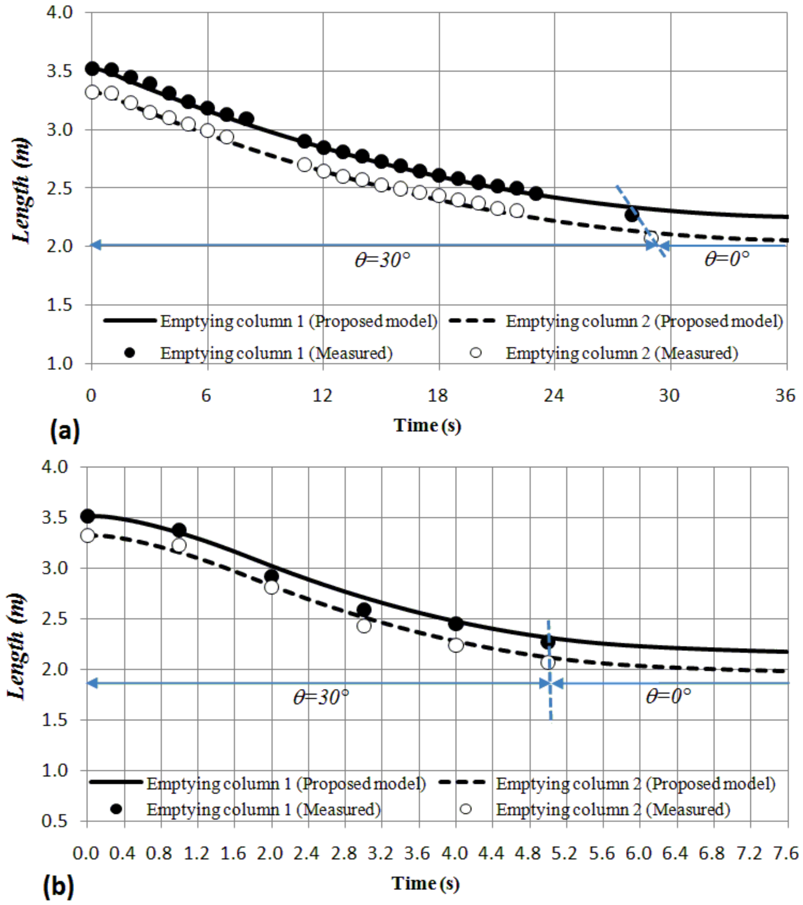
3.2. Experimental Results and Model Verification

Ten experimental tests are selected as shown in

Table 1. Characteristics of tests.

Test No.	Air Valve Model	Air Pocket Length (m)
1	$S050$	$0.001$
2	$S050$	$0.540$
3	$S050$	$0.920$
4	$S050$	$1.320$
5	$S050$	$2.120$
6	$D040$	$0.001$
7	$D040$	$0.540$
8	$D040$	$0.920$
9	$D040$	$1.320$
10	$D040$	$2.120$

, where two different air valves and five air pocket sizes were defined. The air valve $D040$ admits large quantities of air during the emptying process, and it has a diameter of $9.375$ mm and $C_{adm}$ of $0.375$ according to the vacuum curve presented by the manufacturer. The air valve $S050$ is not recommended for vacuum protection because it has a smaller orifice of $3.175$ mm. The manufacturer does not present a vacuum curve because it is used specially for relief in pressurized systems. Consequently, the $C_{adm}$ was calibrated during the tests with a value of $0.303$. The selection of the appropriate air valve size is of utmost importance. The initial air pocket lengths were $0.001$, $0.540$, $0.920$, $1.320$ and $2.120$ m. To avoid a numerical problem in the proposed model, a minimum air pocket size around of 1 mm is imposed instead of 0 mm.

In the model, a constant friction factor of $f=0.018$ was used. Valves $MB{V}_1$ and $MB{V}_2$ were modeled by using a synthetic maneuver, with a flow factor of $K_1=K_2=1.4\times {10}^{-3}$ ${\mathrm{m}}^3/\mathrm{s}$ and a valve maneuvering time ($T_m$) of $1.6$ s. The flow factor represents the local losses due to the opening of the valve and the reduction from $DN63$ to $DN25$. The expansion of the air pocket was modeled by using a polytropic model in adiabatic conditions ($k=1.4$) because the event occurs very quickly.

According to the results, there are two types of behaviours that depend on the air valve: (1) air valve $S050$ (see Figure 5) and (2) air valve $D040$ (see Figure 6). In all tests, the proposed model can predict the subatmospheric pressure pattern. Test No. 1 and Test No. 6 were selected in order to compare results.

Figure 5a shows Test No. 1 (air pocket size of $0.001$ m) where the absolute pressure quickly reaches the minimum subatmospheric pressure of $9.61$ $m_{H20}$ at $1.69$ s. Then, the absolute pressure pattern starts to increase slowly until it reaches the atmospheric condition. The duration of the hydraulic event is $40.3$ s. In contrast, when the air valve $D040$ is used, small troughs of subatmospheric pressure occur and the hydraulic event is very short. Figure 6a shows the results for Test No. 6 (air pocket size of $0.001$ m) where the absolute pressure decreases quickly until it reaches the minimum subatmospheric pressure of $10.16$ $m_{H20}$ at $1.82$ s and then increases again until it reaches the atmospheric condition ($10.33$ $m_{H20}$). The duration of the hydraulic event is $8.13$ s. Figure 5 and Figure 6 show that the pressure drop is linear due to the opening of the valves $MB{V}_1$ and $MB{V}_2$. Then, subatmospheric pressure is presented and the water flow starts to decrease since the air valve can admit a better ratio of the air flow. Consequently, the pressure pattern rises.

In more complex and large systems, an air valve similar to $S050$ cannot be recommended as a protection device during the emptying process because, depending on the conditions of the installation, the subatmospheric pressure can reach excessively low values. Engineers should select an air valve similar to $D040$ for minimizing problems associated with the pressure drop to subatmospheric value.

The density of the air pocket is validated with the measurements of the absolute pressure, since these variables are related, because the temperature of the air pocket remains practically constant. Therefore, the results are similar considering an isothermal process ($k=1.0$).

Figure 7 presents the evolution of the length of emptying columns 1 and 2 for Test No. 2 and Test No. 7. Figure 7a shows the results for Test No. 2 (air valve $S050$) where the emptying column 1 reached the horizontal pipe at 28 s, while the emptying column 2 reached it at 29 s. This difference of 1 s was caused because the valves $MB{V}_1$ and $MB{V}_2$ were not opened exactly at the same time. In contrast, Figure 7 shows the results for Test No. 7 (air valve $D040$), where practically the two emptying column reached the horizontal pipe in 5 s because the hydraulic event in this case is faster. In both tests, the proposed model predicted the length of emptying columns. It is important to note that when the emptying column reaches the horizontal pipe $\theta =0^{\circ }$, the proposed model cannot be applied because air–water interface is parallel to the horizontal pipe direction (as a stratified flow).

Figure 8 shows the comparison between computed and measured water velocity for Test No. 3 and Test No. 8. In both tests, the water velocity in emptying column 1 is practically the same as in emptying column 2 ($v_{e,1}\approx v_{e,2}$). In addition, in all tests from 0 s to $1.6$ s, the water velocity is induced by the opening of the valves $MB{V}_1$ and $MB{V}_2$. In this range of values, the measurements are not adequate because the system starts resting and the UDV cannot detect the suspended small seeding particles because of no reflection. However, after $1.6$ s, the proposed model can predict adequately and give information about the system behaviour. Figure 8a presents the results for Test No. 3 (air valve $S050$) where the maximum water velocity is rapidly reached at $1.39$ s, with a value of $0.076$ m/s. According to the measurements, the maximum value is $0.0775$ m/s at $1.30$ s, which is very close to the proposed model. After the maximum value is attained, the water velocity decreases linearly until it reaches a value of 0 m/s at 34 s. The oscillations around 2 s are caused after the complete opening of valves $MB{V}_1$ and $MB{V}_2$. The water velocity range is very low during the emptying procedure with the air valve $S050$. Consequently, the UDV device with a transducer of 4 MHz frequency cannot detect appropriately the evolution of the water velocity. It records water velocity with intervals of $0.015$ m/s. Figure 8b shows the comparison between computed and measured water velocities for the air valve $D040$ where the water velocity reaches its maximum value of $0.324$ m/s at $1.77$ s. According to the measurements, the maximum value is $0.32$ m/s at $1.78$ s, which is quite similar to the proposed model. After this maximum, the water velocity starts to decrease until the end of the event. During this range, the UDV device can measure appropriately the evolution of the water velocity. The volume of admitted air by $D040$ is almost the same as the water volume drained by valves $MB{V}_1$ and $MB{V}_2$ since the minimum subatmospheric pressure is $10.22$ $m_{H20}$, practically the atmospheric pressure.

3.3. Sensitivity Analysis

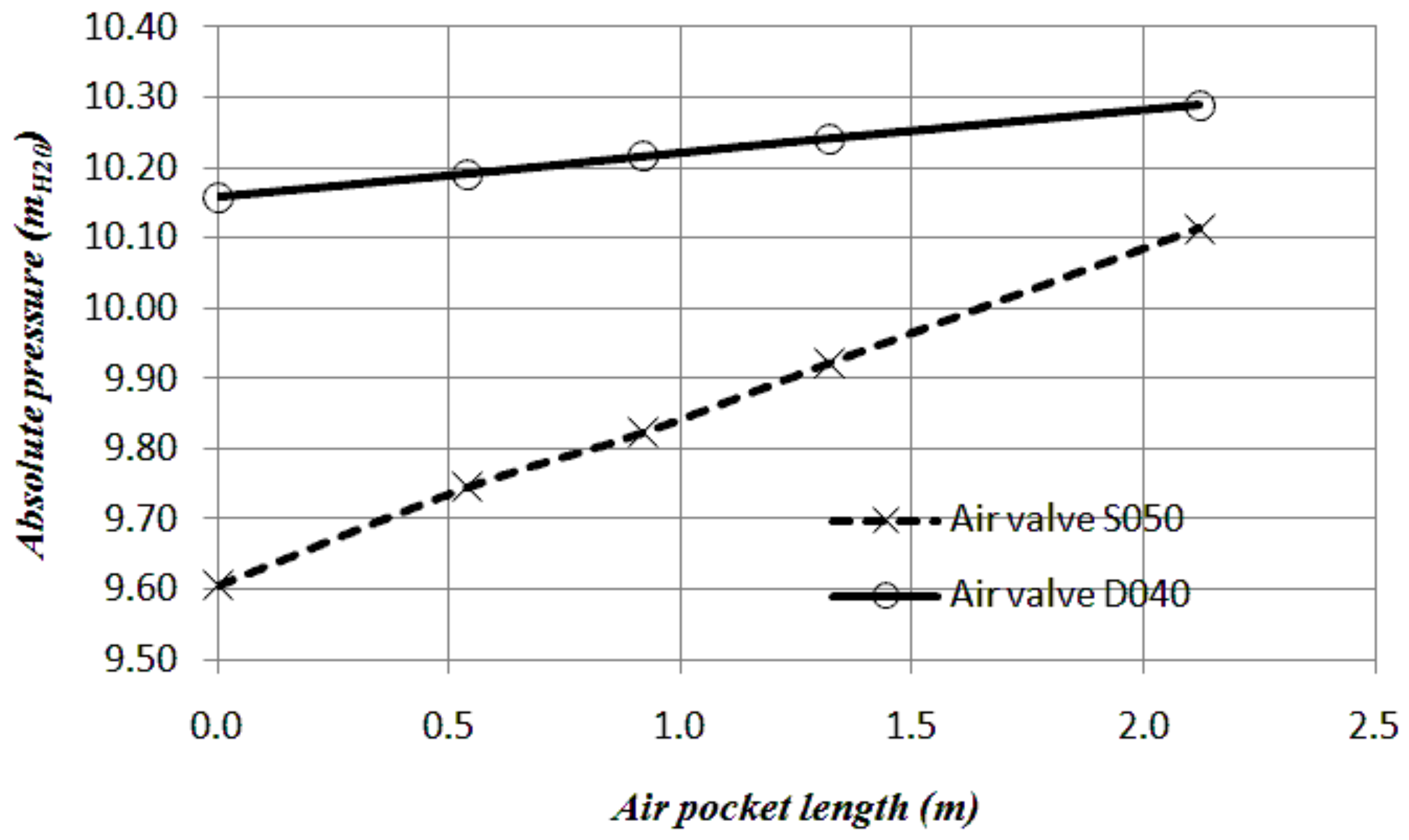
3.3.1. Effect of Air Pocket Sizes

It is important to identify the great influence of the size of the entrapped air pocket on the minimum of the subatmospheric pressure. Figure 9 shows the results taking different air pocket lengths ($0.001$, $0.540$, $0.920$, $1.320$ and $2.120$ m). The smaller the air pocket size, the lower subatmospheric pressure is obtained. Equation (15) shows this situation with the comparison between the gradient of the absolute pressure ($d{p}_i^{*}/dt$) and the air pocket volume ($A_2(L_2-L_{e,2})+A_1(L_1-L_{e,1})$). For the air valve $S050$, subatmospheric pressures are found in the range of 9.61 $m_{H20}$ and 10.11 $m_{H20}$, while, for the air valve $D040$, small variations are found between 10.16 $m_{H20}$ and 10.32 $m_{H20}$, showing the adequacy of this air valve for the emptying process. It also shows the importance of the air valve size since it can induce critical conditions associated with the subatmospheric pressure occurrence.

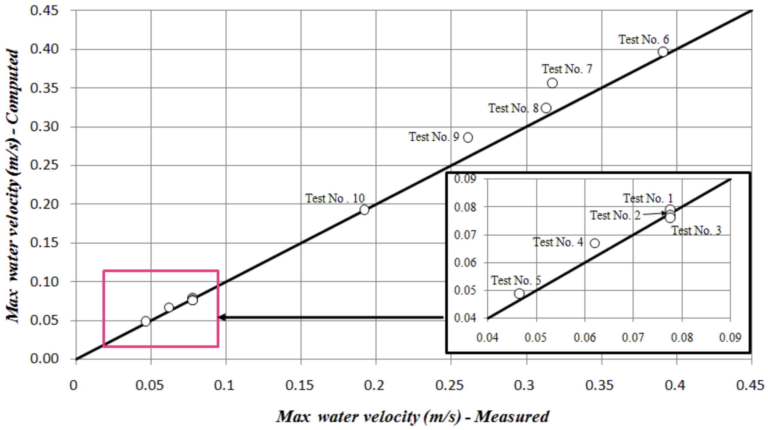
3.3.2. Maximum Water Velocity

Figure 10 shows a comparison between computed and measured maximum water velocities. The proposed model predicts the maximum values of the water velocity for all tests. For the air valve $S050$, maximum values of water velocity are found in the range of $0.049$ to $0.079$ m/s, while, for the air valve $D040$, water velocities are found in the range of $0.193$ to $0.397$ m/s.

4. Conclusions

Subatmospheric pressures occur during the emptying process in pipelines with undulating profiles, which is a typical and common operation that engineers have to face. A rigid two-phase flow model was developed for analyzing it, considering n possible air pockets, d air valves, p pipes, and o drain valves. The proposed model is validated using an experimental facility of an irregular profile of $7.3$ m long and nominal diameter 63 mm ($DN63$), with an air valve located at the high point and several drain valves along the pipeline. The main hydraulic variables could be measured such as flow (both phases), pressure and air-water front position. Comparisons between computed and measured values of the absolute pressure, water velocity and the length of the emptying columns show that the proposed model can predict accurately not only the extreme values but also their patterns. According to the results, the following conclusions can be drawn:

• The proposed model can be used for planning the emptying operations in pipelines with undulating profiles, considering their limitations.
• The expansion of the air pocket produces minimum subatmospheric pressure. In order to control these effects, air valves should be installed in pipelines.
• It is very important to have a correct selection of air valves for vacuum protection for emptying pipelines. An inadequate selection produces both lower values of subatmospheric pressure and a slower drainage of the system. On the other hand, a larger air valve orifice size reduces the lowest values of subatmospheric pressures.
• Engineers should consider the initial condition in which the pipeline is completely filled, which is the most critical condition, since the smallest air pocket sizes produce the lowest subatmospheric pressures.

In real hydraulic pressurized systems, the proposed model can be used for: (i) checking the risk of a system collapse considering factors such as stiffness class, the soil in natural conditions, the type of backfill and the cover depth; and (ii) selecting the air valve sizes depending on the characteristics of each hydraulic system.

References

1. American Water Works Association (AWWA). Manual of Water Supply Practices—M51: Air-Release, Air-Vacuum, and Combination Air Valves, 1st ed.; American Water Works Association: Denver, CO, USA, 2001. [Google Scholar]
2. Ramezani, L.; Karney, B.; Malekpour, A. The Challenge of Air Valves: A Selective Critical Literature Review. J. Water Resour. Plan. Manag. 2016, 141. [Google Scholar] [CrossRef]
3. Fuertes-Miquel, V.S.; Coronado-Hernández, O.E.; Iglesias-Rey, P.L.; Mora-Melia, D. Transient phenomenon during the emptying process of a single pipe with water-air interaction. J. Hydraul. Res. 2016. submitted. [Google Scholar]
4. Tijsseling, A.; Hou, Q.; Bozkuş, Z.; Laanearu, J. Improved One-Dimensional Models for Rapid Emptying and Filling of Pipelines. J. Press. Vessel Technol. 2016, 138, 031301. [Google Scholar] [CrossRef]
5. Laanearu, J.; Annus, I.; Koppel, T.; Bergant, A.; Vučković, S.; Hou, Q.; Tijsseling, A.; Anderson, A.; Van’t Westende, J. Emptying of large-scale pipeline by pressurized air. J. Hydraul. Eng. 2012, 138, 1090–1100. [Google Scholar] [CrossRef]
6. Fuertes, V.S. Hydraulic Transients with Entrapped Air Pockets. Ph.D. Thesis, Department of Hydraulic Engineering, Polytechnic University of Valencia, Valencia, Spain, 2001. [Google Scholar]
7. Besharat, M.; Tarinejad, R.; Ramos, H.M. The effect of water hammer on a confined air pocket towards flow energy storage system. J. Water Supply Res. Technol. AQUA 2016, 65, 116–126. [Google Scholar] [CrossRef]
8. Apollonio, C.; Balacco, G.; Fontana, N.; Giugni, M.; Marini, G.; Piccinni, A.F. Hydraulic Transients Caused by Air Expulsion during Rapid Filling of Undulating Pipelines. Water 2016, 8, 25. [Google Scholar] [CrossRef]
9. Balacco, G.; Apollonio, C.; Piccinni, A.F. Experimental Analysis of Air Valve Behaviour During Hydraulic Transients. J. Appl. Water Eng. Res. 2015, 3, 3–11. [Google Scholar] [CrossRef]
10. Zhou, L.; Liu, D.; Karney, B. Investigation of hydraulic transients of two entrapped air pockets in a water pipeline. J. Hydraul. Eng. 2013, 139, 949–959. [Google Scholar] [CrossRef]
11. Izquierdo, J.; Fuertes, V.S.; Cabrera, E.; Iglesias, P.; García-Serra, J. Pipeline start-up with entrapped air. J. Hydraul. Res. 1999, 37, 579–590. [Google Scholar] [CrossRef]
12. Zhou, L.; Liu, D.; Ou, C. Simulation of flow transients in a water filling pipe containing entrapped air pocket with VOF model. Eng. Appl. Comput. Fluid Mech. 2011, 5, 127–140. [Google Scholar] [CrossRef]
13. Martins, N.M.C.; Soares, A.K.; Ramos, H.M.; Covas, D.I.C. CFD modeling of transient flow in pressurized pipes. Comput. Fluids 2016, 126, 129–140. [Google Scholar] [CrossRef]
14. Abreu, J.; Cabrera, E.; Izquierdo, J.; García-Serra, J. Flow Modeling in Pressurized Systmes Revisited. J. Hydraul. Eng. 1999, 125, 1154–1169. [Google Scholar] [CrossRef]
15. Martins, S.C.; Ramos, H.M.; Almeida, A.B. Mathematical Modeling of Pressurized System Behaviour with Entrapped Air. In Environmental Hydraulics: Theoretical, Experimental and Computational Solutions; CRC Press: Boca Raton, FL, USA, 2010; pp. 61–64. [Google Scholar]
16. Martins, S.C.; Ramos, H.M.; Almeida, A.B. Computational Evaluation of Hydraulic System Behaviour with Entrapped Air under Rapid Pressurization; Integrating Water Systems; CRC Press: Boca Raton, FL, USA, 2010; pp. 241–247. [Google Scholar]
17. Fuertes-Miquel, V.S.; López-Jiménez, P.A.; Martínez-Solano, F.J.; López-Patiño, G. Numerical modelling of pipelines with air pockets and air valves. Can. J. Civ. Eng. 2016, 43, 1052–1061. [Google Scholar] [CrossRef]
18. Zhou, L.; Liu, D. Experimental investigation of entrapped air pocket in a partially full water pipe. J. Hydraul. Res. 2013, 51, 469–474. [Google Scholar] [CrossRef]
19. Covas, D.; Stoianov, I.; Ramos, H.M.; Graham, N.; Maksimovic̀, C.; Butler, D. Water hammer in pressurized polyethylene pipes:conceptual model and experimental analysis. Urban Water J. 2010, 1, 177–197. [Google Scholar] [CrossRef]
20. Liou, C.; Hunt, W.A. Filling of pipelines with undulating elevation profiles. J. Hydraul. Eng. 1996, 122, 534–539. [Google Scholar] [CrossRef]
21. Bousso, S.; Daynou, M.; Fuamba, M. Numerical Modeling of Mixed Flows in Storm Water Systems: Critical Review of Literature. J. Hydraul. Eng. 2013, 139, 385–396. [Google Scholar] [CrossRef]
22. Leon, A.; Ghidaoui, M.; Schmidt, A.; Garcia, M. A robust two-equation model for transient-mixed flows. J. Hydraul. Res. 2010, 48, 44–56. [Google Scholar] [CrossRef]
23. Wylie, E.; Streeter, V. Fluid Transients in Systems; Prentice Hall: Englewood Cliffs, NJ, USA, 1993. [Google Scholar]
24. Vasconcelos, J.G.; Wright, S.J. Rapid Flow Startup in Filled Horizontal Pipelines. J. Hydraul. Eng. 2008, 134, 984–992. [Google Scholar] [CrossRef]
25. Cabrera, E.; Abreu, J.; Pérez, R.; Vela, A. Influence of Liquid Length Variation in Hydraulic Transients. J. Hydraul. Res. 1992, 118, 1639–1650. [Google Scholar] [CrossRef]
26. Zhou, L.; Liu, D.; Karney, B. Phenomenon of white mist in pipelines rapidly filling with water with entrapped air pocket. J. Hydraul. Eng. 2013, 139, 1041–1051. [Google Scholar] [CrossRef]
27. Martins, S.C.; Ramos, H.M.; Almeida, A.B. Conceptual analogy for modelling entrapped air action in hydraulic systems. J. Hydraul. Res. 2015, 53, 678–686. [Google Scholar] [CrossRef]
28. Martin, C.S. Entrapped Air in Pipelines. In Proceedings of the Second International Conference on Pressure Surges, London, UK, 22–24 September 1976.
29. Iglesias-Rey, P.L.; Fuertes-Miquel, V.S.; García-Mares, F.J.; Martínez-Solano, F.J. Comparative Study of Intake and Exhaust Air Flows of Different Commercial Air Valves. In Proceedings of the 16th Conference on Water Distribution System Analysis, WDSA 2014, Bari, Italy, 14–17 July 2014; pp. 1412–1419.
Figure 1. Scheme of entrapped air pockets in a pipeline with irregular profile while water empties.
Water 09 00098 g001
Figure 2. Evolution of the gravity term of the emptying column j.
Water 09 00098 g002
Figure 3. Two emptying columns in a pipeline.
Water 09 00098 g003
Figure 4. The pipe system and its components.
Water 09 00098 g004
Figure 5. Comparison between computed and measured absolute pressure oscillation patterns (air valve S050): (a) Test No. 1; (b) Test No. 2; (c) Test No. 3; (d) Test No. 4; (e) Test No. 5.
Water 09 00098 g005
Figure 6. Comparison between computed and measured absolute pressure oscillation patterns (air valve D040): (a) Test No. 6; (b) Test No. 7; (c) Test No. 8; (d) Test No. 9; (e) Test No. 10.
Water 09 00098 g006
Figure 7. Comparison between computed and measured length of emptying columns: (a) Test No. 2 (air valve S 050 ); (b) Test No. 7 (air valve D 040 ).
Water 09 00098 g007
Figure 8. Comparison of water velocity between computed and measured values: (a) Test No. 3 (air valve S 050 ); (b) Test No. 8 (air valve D 040 ).
Water 09 00098 g008
Figure 9. Effect of the air pocket sizes on the minimum pressure attained.
Water 09 00098 g009
Figure 10. Comparison between computed and measured maximum water velocities.
Water 09 00098 g010