An EMD-Based Chaotic Least Squares Support Vector Machine Hybrid Model for Annual Runoff Forecasting

Abstract

Accurate forecasting of annual runoff is necessary for water resources management. However, a runoff series consists of complex nonlinear and non-stationary characteristics, which makes forecasting difficult. To contribute towards improved prediction accuracy, a novel hybrid model based on the empirical mode decomposition (EMD) for annual runoff forecasting is proposed and applied in this paper. Firstly, the original annual runoff series is decomposed into a limited number of intrinsic mode functions (IMFs) and one trend term based on the EMD, which makes the series stationary. Secondly, it will be forecasted by a least squares support vector machine (LSSVM) when the IMF component possesses chaotic characteristics, and simulated by a polynomial method when it does not. In addition, the reserved trend term is predicted by a Gray Model. Finally, the ensemble forecast for the original runoff series is formulated by combining the prediction results of the modeled IMFs and the trend term. Qualified rate (QR), root mean square errors (RMSE), mean absolute relative errors (MARE), and mean absolute errors (MAE) are used as the comparison criteria. The results reveal that the EMD-based chaotic LSSVM (EMD-CLSSVM) hybrid model is a superior alternative to the CLSSVM hybrid model for forecasting annual runoff at Shangjingyou station, reducing the RMSE, MARE, and MAE by 39%, 28.6%, and 25.6%, respectively. To further illustrate the stability and representativeness of the EMD-CLSSVM hybrid model, runoff data at three additional sites, Zhaishang, Fenhe reservoir, and Lancun stations, were applied to verify the model. The results show that the EMD-CLSSVM hybrid model proved its applicability with high prediction precision. This approach may be used in similar hydrological conditions.

1. Introduction

Runoff forecasting, especially annual runoff forecasting, is required for appropriate and effective water resource planning and management [1,2]. It is generally known that the processes of runoff generation are heavily influenced by a host of factors such as precipitation, temperature, evaporation, underlying surface, and human activity [3,4]. Due to the uncertainty of these factors, runoff series tend to be nonlinear, non-stationary, and even chaotic [5,6]. It is very difficult to make accurate predictions about annual runoff, which has been a challenge for hydrologists over years.

In the past two decades, the characteristic of deterministic chaos in runoff series has been observed by some researchers [7,8,9]. When the runoff series possesses a chaotic trait, the conventional forecasting methods may not function properly. Recently, chaos-based runoff forecasting techniques have become increasingly attractive to the hydrology community [10,11]. Generally, the key to chaotic time series prediction is the phase space reconstruction theory, which is not concerned with whether a time series is stationary or not. Many studies have shown that once the time series has chaotic attractor, the phase space can be reconstructed when the appropriate parameters are chosen [12,13]. However, a reconstruction process may be affected by the non-stationary characteristics of the runoff series. A general method to deal with the non-stationarity is to apply the finite difference method (FDM) to the runoff series in question [14]. However, the series processed by using FDM may not remain stationary. In view of this, an empirical mode decomposition (EMD) has recently been introduced. The EMD method can self-adaptively decompose a complex non-stationary and nonlinear series into several intrinsic mode functions (IMFs). The EMD-based hybrid models have been successfully employed to predict runoff series [15,16]. However, many researchers only consider EMD a useful tool for the analysis of multi-scale variations of the runoff series [17,18], and have paid little attention to converting non-stationary runoff series into stationary ones. In this paper, the EMD method is introduced to make the time series stationary.

Due to the nonlinear and chaotic characteristics of the runoff series, artificial intelligence appears to be a useful alternative to conventional statistical techniques for forecasting runoff, such as artificial neural networks (ANNs), support vector machines (SVM), and least squares support vector machines (LSSVM). Previous studies have demonstrated that ANNs are useful for runoff series forecasting [19,20]. However, the ANNs were subject to local convergence, slow learning, and poor generalization ability, which led to unsatisfactory performance. By contrast, the SVM is characterized by having non-linear kernels, high generalization ability, and sparse solutions, which is useful for forecasting small sample cases. The SVM is based on the structural risk minimization induction principle rather than the empirical risk minimization, and can achieve the global optimum by solving a quadratic optimization problem. The SVM is currently used increasingly in forecasting runoff series [21,22], although this method is often time-consuming and has a higher computational burden due to the requisite constrained optimization programming. To reduce the complexity of the optimization process, the LSSVM is proposed, which has also been successfully employed in runoff forecasting [23,24]. It adopts equality constraints rather than inequality constraints and uses the least squares linear system as its loss functions, which makes it computationally easier. The LSSVM presents similar advantages over the SVM, but an additional advantage of the LSSVM is that it only requires solving a set of linear equations rather than quadratic programming. Therefore, this paper presents an algorithm aimed at achieving accurate forecasts of annual runoff based on the combination of the EMD and chaotic least squares support vector machine (EMD-CLSSVM), which means that the original annual runoff time series are transformed into stationary subseries by EMD; subseries would be predicted by LSSVM when it has chaotic characteristics, and by a polynomial method when it does not.

The main objective of this paper is to apply the EMD-CLSSVM hybrid model for annual runoff series forecasting under the case studies in the upper reaches of the Fenhe River basin, China. First, the EMD is applied to decompose the original annual runoff data into several IMFs and one trend term. Secondly, the stationarity of these IMFs was tested based on the KSPP method. Thirdly, the chaotic characteristics of the IMFs were identified based on the largest Lyapunov exponent method. The IMFs and the trend term were then modeled and forecasted using the CLSSVM, polynomial method, and Gray Model (GM). Finally, these prediction results are integrated to get the final annual runoff forecasting values. The EMD-CLSSVM hybrid model is compared to the CLSSVM hybrid approach to find a reliable hybrid forecasting model for annual runoff series.

2. Data and Methods

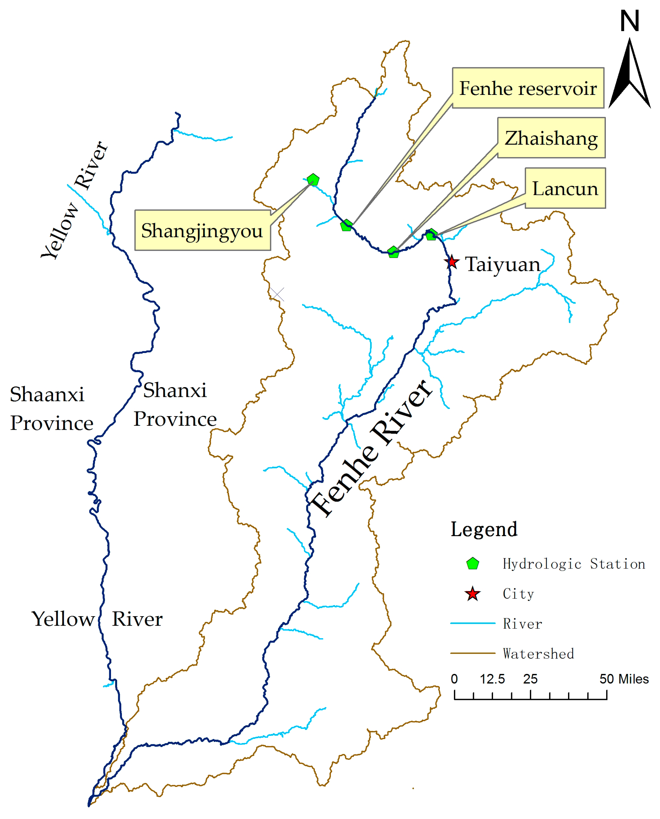
2.1. Study Area and Data

The Fenhe River is located in the North China (110° E–114° E, 35° N–39° N), which covers a drainage area of about 38,728 km² with a river length of 716 km, as seen in Figure 1. With a semi-arid climate, the Fenhe River basin has an average annual precipitation ranging from 300 to 750 mm and an annual mean temperature varying from 9 to 12 °C. The upper reaches of the Fenhe River are in the area above Lancun station. Annual runoff data from four hydrologic stations in the upper reaches, i.e., Shangjingyou, Fenhe reservoir, Zhaishang, and Lancun, were analyzed. Shangjingyou station lies in Lan River, which belongs to one of the tributaries of Fenhe River. The Zhaishang, Fenhe reservoir, and Lancun stations are in the mainstream of Fenhe River. The locations of the stations are shown in Figure 1. These runoff data of flow records covering 1956 to 2000 were obtained from the government hydrologic database. The first 40 years (1956–1995) of runoff data were applied for calibration purpose and the remaining five years of data were used for validation.

2.2. Methods

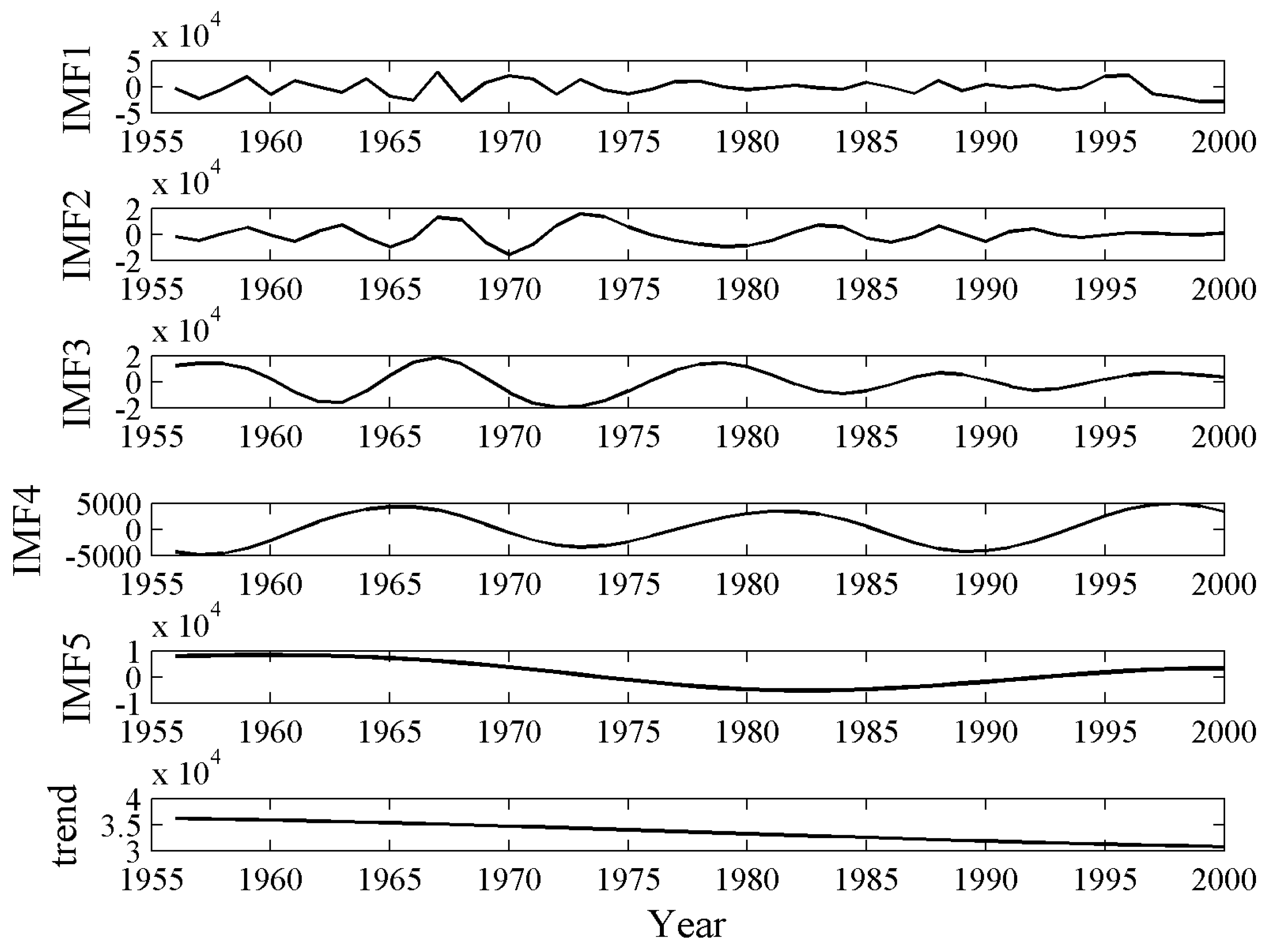
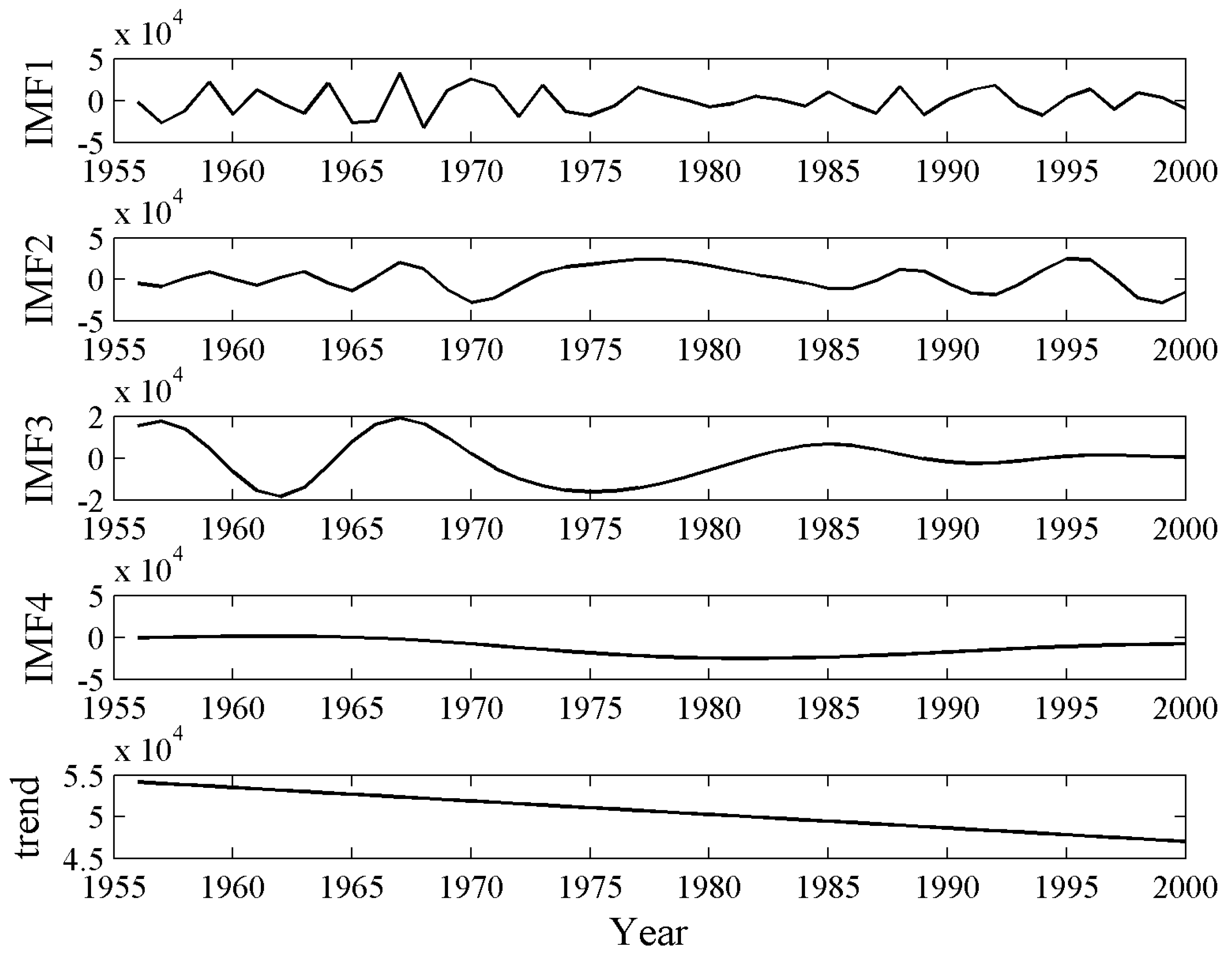
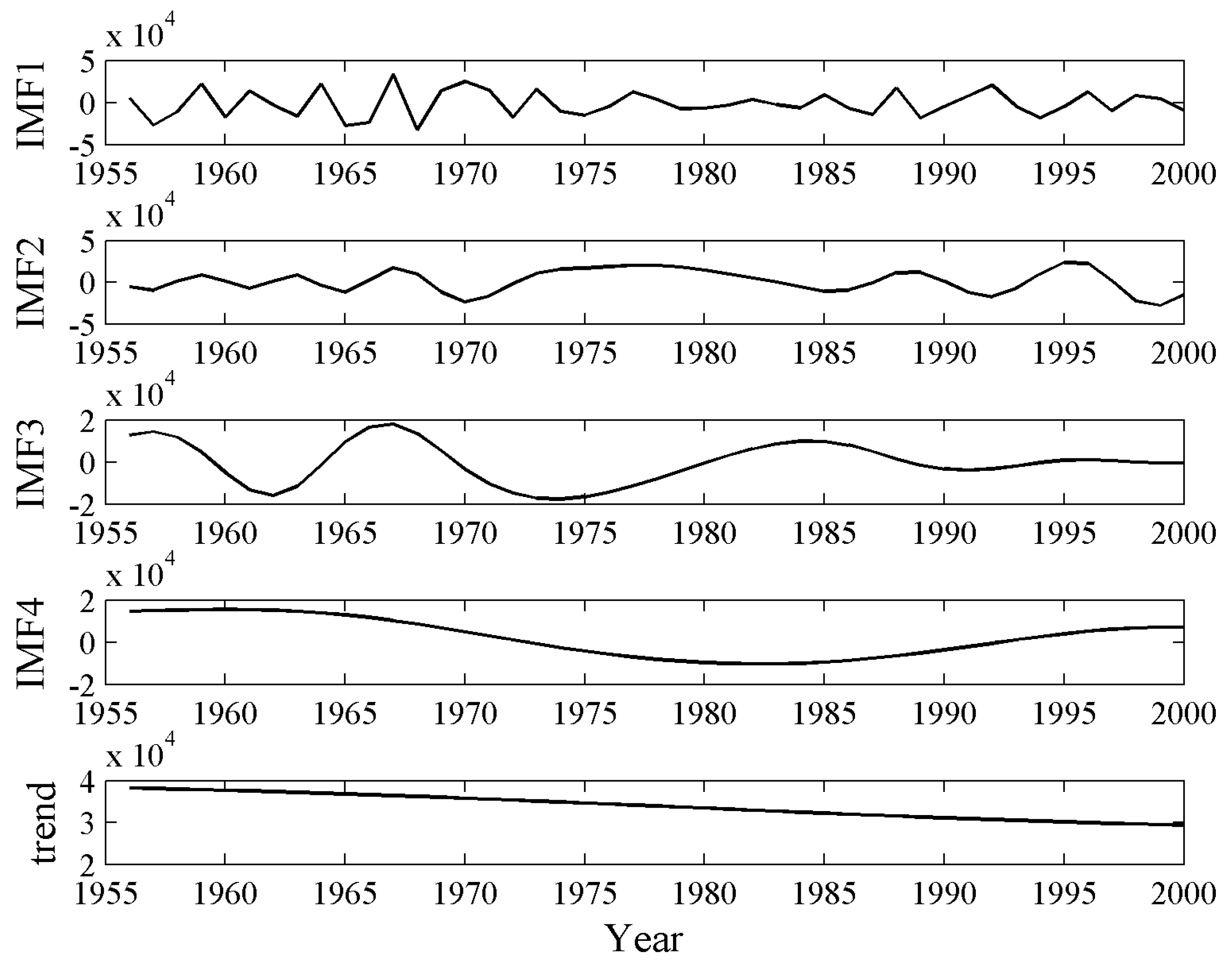
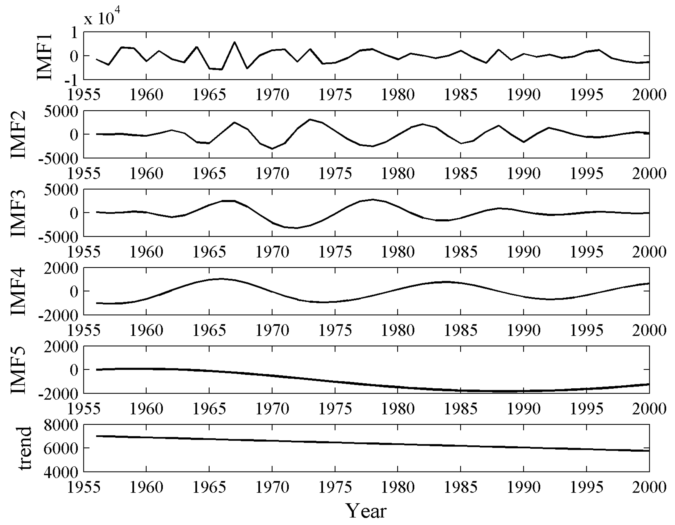
2.2.1. Empirical Mode Decomposition

EMD is an effective method used for the analysis of non-stationary time series [25]. The most important feature of EMD is that it can adaptively decompose the non-stationary runoff series into several stationary IMFs and a trend term. The IMFs are produced by an iterative process called sifting. Sifting is the core of the EMD method. The sifting process is summarized as follows:

Step 1)

Identify all the extreme (maxima and minima) values of a time series $x(t)$.

Step 2)

Generate the upper and lower envelope ($u(t)$ and $v(t)$) by applying cubic spline interpolation.

Step 3)

Compute a local mean curve $m(t)$ of the two envelopes at the same time using

$$m(t)=(u(t)+v(t))/2.$$

(1)

Step 4)

Calculate the difference,

$$h(t)=x(t)-m(t).$$

(2)

Step 5)

Check the properties of $h(t)$; it will be considered a valid IMF if it satisfies these two conditions:

• The number of extreme and zero crossings must be equal or differ at most by one.
• At any point, the local mean value of the envelope defined by the local extremes must be zero.

Step 6)

When $h(t)$ is not qualified as an IMF, repeat Steps 1) to 5) by sifting the residual series. The sifting process stops when the residual (i.e., the trend term; $r(t)$) satisfies the predetermined criteria.

Finally, the input runoff series can be decomposed into several IMFs and a residual $r(t)$ as follows. In addition, the original runoff series $x(t)$ can be exactly reconstructed by the following linear superposition:

$$x(t)={\displaystyle \sum _{i=1}^{n}h(t)+r(t)},$$

(3)

where h(t) is the IMF, r(t) refers to the residual term, and n is the number of IMFs.

2.2.2. Phase Space Reconstruction and Chaotic Characteristics Identification

The phase space is the space of all possible states of a system with the observed data. Phase space reconstruction is the prerequisite for predictions of time series. To describe the temporal evolution of a time series in a multi-dimensional phase space, it is essential to unfold a multi-dimensional structure using univariate data, i.e., the one-dimensional time series is embedded to multi-dimensional phase space through reconstruction. For a time series $\left\{x_1,x_2,\cdots ,x_n\right\}$, it may be reconstructed into a series of delay vectors of the following type:

$$y_i=\left\{x_i,x_{i+\tau },x_{i+2\tau },\cdots ,x_{i+(m-1)\tau }\right\},i=1,2,\cdots ,n-(m-1)\tau ,$$

(4)

where $y_i$ is a point of m-dimensional phase space, m is the embedding dimension, and τ is the delay time. The connection of $n-(m-1)\tau$ points describes the evolution orbit of the system in m-dimensional phase space. By means of phase space reconstruction, it is hoped that the points in m-dimensional phase space form an attractor that is defined as regular phase space orbit. In theory, a good reconstruction means near topological equivalence of the reconstructed attractor to the original one.

The selection of τ and m is important for the quality of the reconstruction. Delay time τ is usually calculated by the autocorrelation function method, the multiple correlation function method, and the mutual information method [26]. The autocorrelation function method is mainly used to measure the linear correlation of a continuous time series. However, when the time series is nonlinear, this method will be ineffective. The mutual information method, based on Shannon information entropy, can not only be used to calculate the correlation between variables, but also to provide measurement of the overall dependence of variables. This method can be used to analyze the linear correlation as well as the nonlinear correlation. Therefore, in this paper, the mutual information method is employed to determine the delay time τ. The typical methods of determining embedding dimension m include the Grassberger–Procaccia algorithm, correlation integral, false nearest neighbor (FNN) [27], and the Cao method [28]. Generally, the saturated correlation dimension method requires a larger sample. The FNN method will obtain different false nearest points when the threshold value selection is different. Hence, the Cao method is adopted to determinate the embedding dimension in this paper.

If a time series is non-stationary, the phase space reconstruction method is robust. It is necessary to transform the time series into stationary ones before selecting the parameters of phase space. The KPSS method introduced by Kwiatkowski, Phillips, Schmidt and Shin [29] is used to test the stationarity of a time series.

Let $y_t$, t = 1, 2, …, N, be the time series for which we wish to test stationarity. Let $e_t$, t = 1, 2, …, N be the residuals from the regression of $y$ on an intercept and time trend. Let ${\widehat{\sigma }}_{\epsilon }^2$ be the estimate of the error variance from this regression (the sum of squared residuals, divided by N). Define the partial sum process of the residuals:

$$S_t={\displaystyle \sum _{i=1}^t{e}_i},t=1,2,\dots ,N.$$

(5)

The Lagrange Multiplier (LM) statistic is

$$LM={\displaystyle \sum _{t=1}^N{S}_t^2/{\widehat{\sigma }}_{\epsilon }^2}.$$

(6)

The null hypothesis of this test is stationary series. Thus if the LM statistic value is greater than the critical value (chosen alpha level), the null hypothesis is rejected. On the contrary, if the LM statistic value is less than the critical value, the null hypothesis cannot be rejected.

The diagnosis of the character of chaos can begin when the phase space has been reconstructed. Chaotic characteristics identification is significant to reveal the essential law of runoff series and establish a reliable forecasting model. The usual methods of chaotic characteristics identification include the phase portrait, power spectrum, saturated correlation dimension, largest Lyapunov exponent, Kolmogorov entropy, and so on [30]. The largest Lyapunov exponent is employed to identify the chaotic characteristics in this paper.

2.2.3. Chaotic Least Squares Support Vector Machine Model

Given the training samples $X_t=\left\{x_1,x_2,\cdots ,x_n\right\}$, if we choose the proper delay time τ, embed dimension m, and transform the prediction series $X_t$ into new m dimension data space, it may be expressed as follows:

$$\left[\begin{array}{c}{\mathit{X}}_1\\ {\mathit{X}}_2\\ ⋮\\ {\mathit{X}}_{\mathit{M}}\end{array}\right]=\left[\begin{array}{ccccc}{x}_1& x_{1+\tau }& x_{1+2\tau }& \cdots & x_{1+(m-1)\tau }\\ x_2& x_{2+\tau }& x_{2+2\tau }& \cdots & x_{2+(m-1)\tau }\\ ⋮& ⋮& ⋮& ⋮& ⋮\\ x_M& x_{M+\tau }& x_{M+2\tau }& \cdots & x_{M+(m-1)\tau }\end{array}\right],$$

(7)

where $M=n-(m-1)\tau$, $X_2=F(X_1)$, $X_3=F(X_2)$, …, $X_M=F(X_{M-1})$, and the relation is:

$${\mathit{X}}_{t+1}=\{x_{t+1},x_{t+1+\tau },x_{t+1+2\tau },\cdots ,x_{t+1+(m-1)\tau }\}=F(x_t,x_{t+\tau },x_{t+2\tau },\cdots ,x_{t+(m-1)\tau }).$$

(8)

The former $m-1$ dimension of $X_{t+1}$ is as in the historic data, which is converted into a single output as follows:

$$x_{t+1+(m-1)\tau }=f(x_t,x_{t+\tau },x_{t+2\tau },\cdots ,x_{t+(m-1)\tau }),$$

(9)

where $f(x)$ is the mapping from $R^m$ to $R$. The essence of the prediction problem is to obtain a best approximation of $f(x)$, which has high nonlinearity. Therefore, a nonlinear function is adopted to fit the mapping. Combined with the LSSVM model, training data is obtained as follows:

$$\mathit{Y}={[\begin{array}{cccc}{x}_{2+(m-1)\tau }& x_{3+(m-1)\tau }& \cdots & x_{M+1+(m-1)\tau }\end{array}]}^T.$$

(10)

Assuming the current training sample is as shown in Equation (10), the length of the time window is $M$. When one new series comes into the time window, the oldest series $X_1$ is removed. Therefore, the training series goes back to the form of Equation (10) again. Using the LSSVM algorithm, the current regression function is given as follows:

$$f(x)={\displaystyle \sum _{i=1}^M{\alpha }_{i}K(x_i,x)+b}.$$

(11)

Furthermore, the result of the first prediction step is

$${\widehat{x}}_{M+2+(m-1)\tau }={\displaystyle \sum _{i=1}^M{\alpha }_{i}K(x_i,X_{M+1})+b},$$

(12)

where ${\mathit{X}}_{M+1}=[x_{M+1},x_{M+1+\tau },x_{M+1+2\tau },\cdots ,x_{M+1+(m-1)\tau }]$.

Thus, the result of p step prediction model is,

$${\widehat{x}}_{M+p+1+(m-1)\tau }={\displaystyle \sum _{i=1}^M{\alpha }_{i}K(x_i,X_{M+p})+b},$$

(13)

where ${\mathit{X}}_{M+p}=[x_{M+p},x_{M+p+\tau },x_{M+p+2\tau },\cdots ,x_{M+p+(m-1)\tau }]$.

3. Model Results and Discussion

3.1. Stationarity Test of the Original Runoff Series

In order to examine the stationarity of a runoff series, the KPSS method is used to test the stationarity of the original runoff series. The result indicates that the LM statistic value (0.847) of the annual runoff series for Shangjingyou hydrologic station is greater than the critical value (0.463), which shows that the annual runoff series for Shangjingyou station is non-stationary. Therefore, it is necessary to transform the runoff series to become stationary.

3.2. EMD of Runoff Series

The original runoff series are decomposed into several sub-series over the same time domain, namely, IMF1 to IMF5, and one trend term based on the EMD for Shangjingyou hydrologic station, as seen in Figure 2.

The KPSS is also used to analyze the stationarity of IMFs. As shown in

Table 1. Lagrange Multiplier (LM) statistic, delay time τ, embedding dimension m, average period p, and Lyapunov exponent λ₁ of intrinsic mode functions (IMFs) for Shangjingyou station.

IMFs	LM Statistic	τ	m	Average Period p	Lyapunov Exponent λ1
IMF1	0.114	1	2	3	0.113
IMF2	0.148	1	5	4	0.160
IMF3	0.063	2	4	4	0.101
IMF4	0.075	4	6	8	0.040
IMF5	0.571	1	6	23	—

, the LM statistic value of several IMFs for Shangjingyou station are all less than the critical value, which indicates the runoff series decomposed by the EMD become stationary ones.

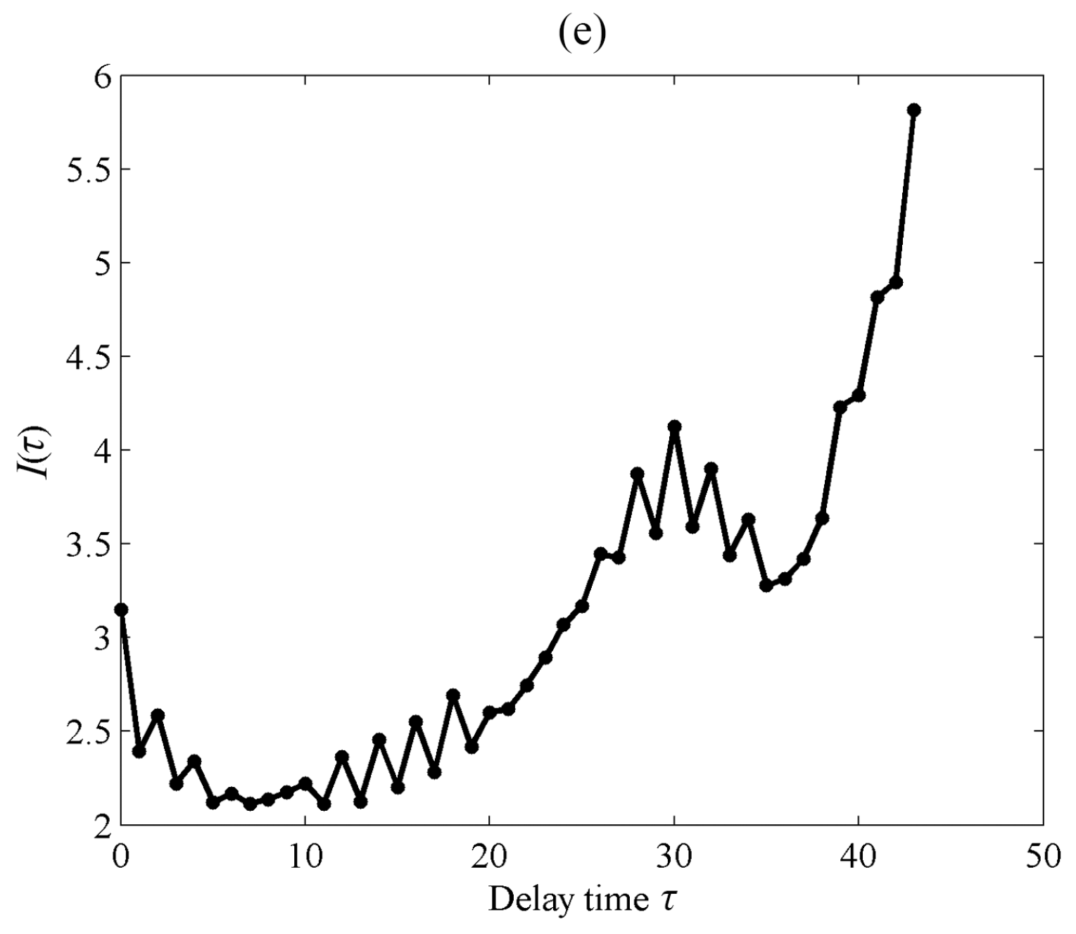
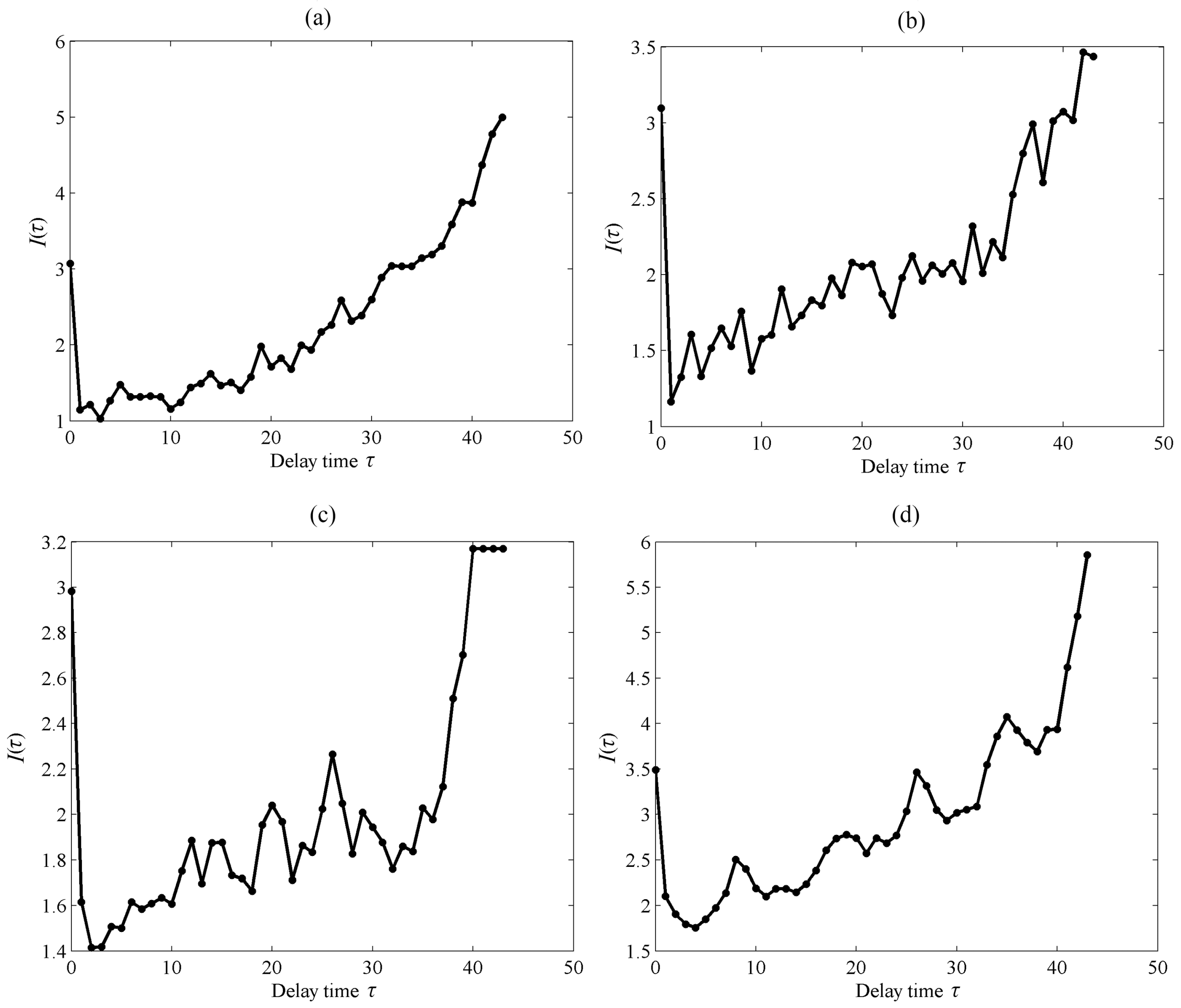
3.3. Determination of Delay Time τ and Embedding Dimension m

Figure 3 indicates the mutual information $I(\tau )$ of IMF1, IMF2, IMF3, IMF4, and IMF5 for Shangjingyou station. $I(\tau )$ for each runoff series is the minimum attained firstly at the lag time of 1, 1, 2, 4, and 1. Therefore, the five values of the delay time τ for IMF1, IMF2, IMF3, IMF4, and IMF5 at Shangjingyou station are chosen as 1, 1, 2, 4, and 1, respectively (Table 1). The embedding dimension m of the IMFs for Shangjingyou station, as determined by the Cao method, is shown in Table 1.

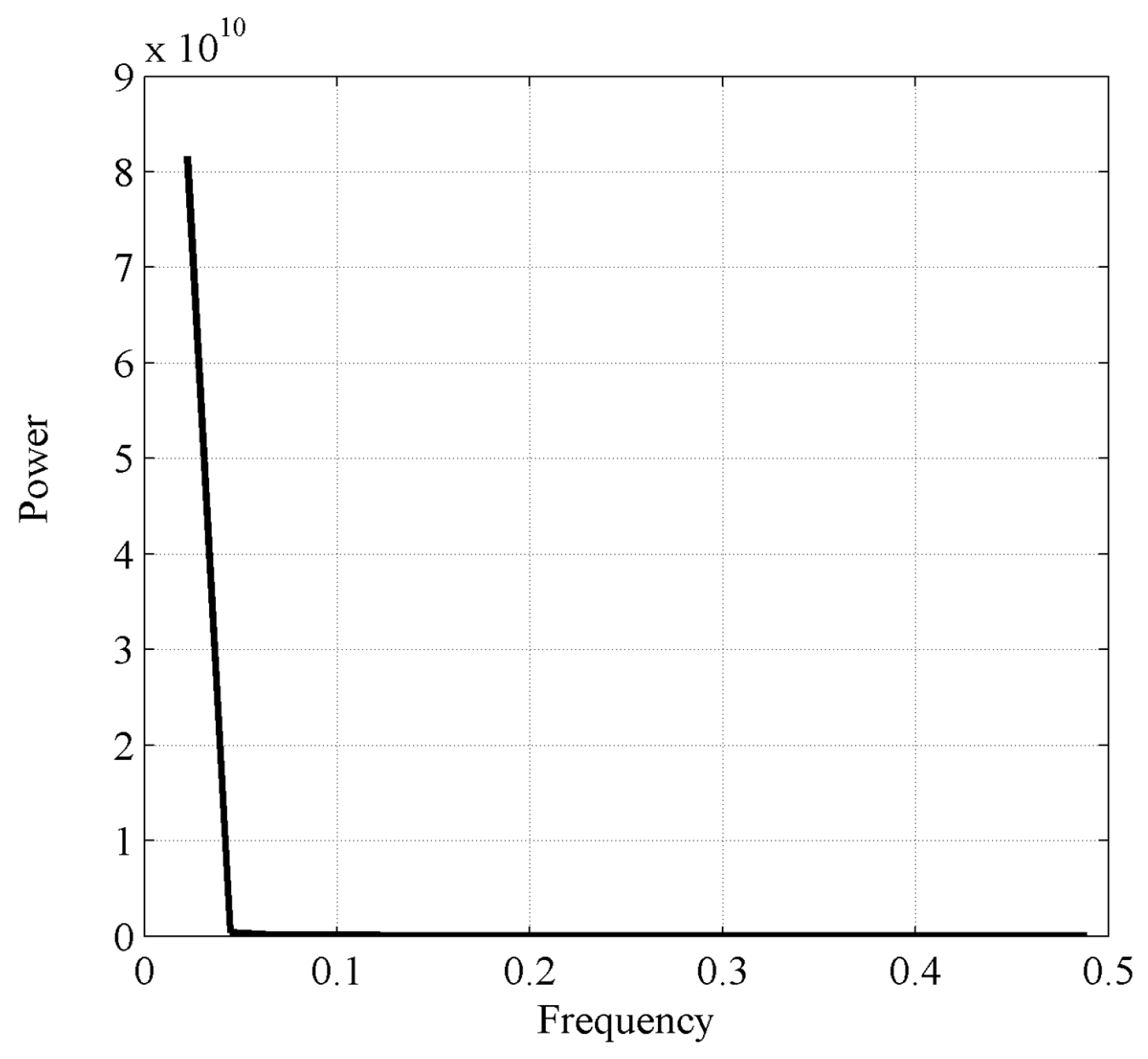
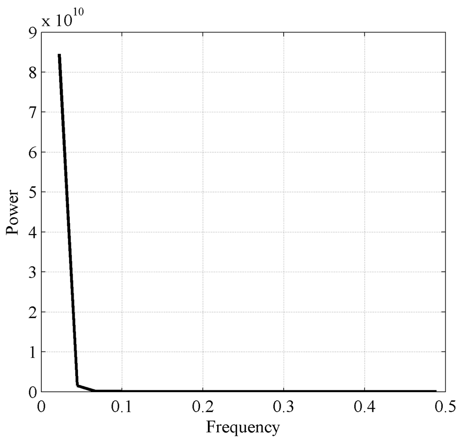
3.4. Identification of Chaotic Characteristics

The average periods of several IMFs for Shangjingyou station need to be determined before identifying the chaotic characteristics by the largest Lyapunov exponent method. Therefore, the Hilbert transform [25] is used to calculate the average period p with the results shown in Table 1.

The largest Lyapunov exponent is used to identify the chaotic characteristics of IMFs for Shangjingyou station. It can be seen in Table 1 that the Lyapunov exponent λ₁ of IMFs for Shangjingyou station is greater than zero, except for IMF5, which indicates that IMFs have chaotic characteristics. The average period of the IMF5 for Shangjingyou station was 23 years, but the lengths of IMF5 for Shangjingyou station are only 45 years. Therefore, the Lyapunov exponent method would be unable to analyze the chaotic characteristics of the IMF5. In view of this, the Power Spectrum method is used to analyze the chaotic characteristics of the IMF5 for Shangjingyou station. Figure 4 shows that the IMF5 for Shangjingyou station has a single peak, which indicates that the IMF5 time series does not have chaotic characteristics.

Chaotic characteristics are only found from IMF1, IMF2, IMF3, and IMF4 for Shangjingyou station. The IMF5 for Shangjingyou station has no chaotic characteristics.

3.5. Hybrid Model

For the chaotic time series, after the phase space reconstruction, the LSSVM model is trained by the reconstructed learning samples. The parameters of the LSSVM model include C, ε, and σ, where ε decides the SVM number and model generalization. The greater the value of ε, the lower the number of SVM and the worse the model precision. ε is taken to be 0.001 in this paper. The parameters of C and σ jointly control the model complexity and prediction accuracy. In the calculation, the Bayesian Information Criterion (BIC) is used to optimally select the parameters of C and σ. The selected parameters are shown in

Table 2. Least squares support vector machine (LSSVM) model parameters of IMFs for Shangjingyou station. C: penalty factor; σ: parameter of kernel function.

IMFs	IMF1	IMF2	IMF3	IMF4
C	625.2	316.0	68.1	18.1
σ	0.1	49.2	7.2	8.3

.

The CLSSVM is used to train and test the IMF1, IMF2, IMF3, and IMF4 for Shangjingyou station. The polynomial method is employed to model and forecast the last IMF for Shangjingyou station, and the GM is applied to predict the trend term. Finally, the resultant predictions of the modeled IMFs and trend term are summed to formulate an ensemble forecast for the original runoff series. In order to further prove the superiority of the EMD-CLSSVM hybrid model over the others, the CLSSVM hybrid model was employed as a comparative forecast model to predict the annual runoff, which means that in place of the EMD-CLSSVM model, the CLSSVM model is used with other models unchanged. The prediction results are shown in Figure 5. It can be seen from the hydrographs that the EMD-CLSSVM hybrid model shows better performance for annual runoff forecasting compared with the CLSSVM hybrid model in the testing period.

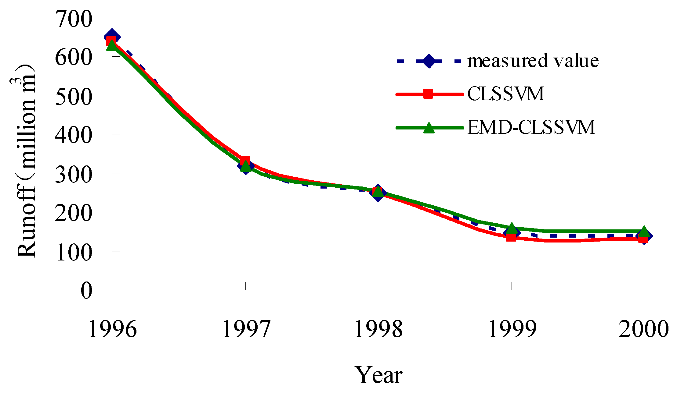
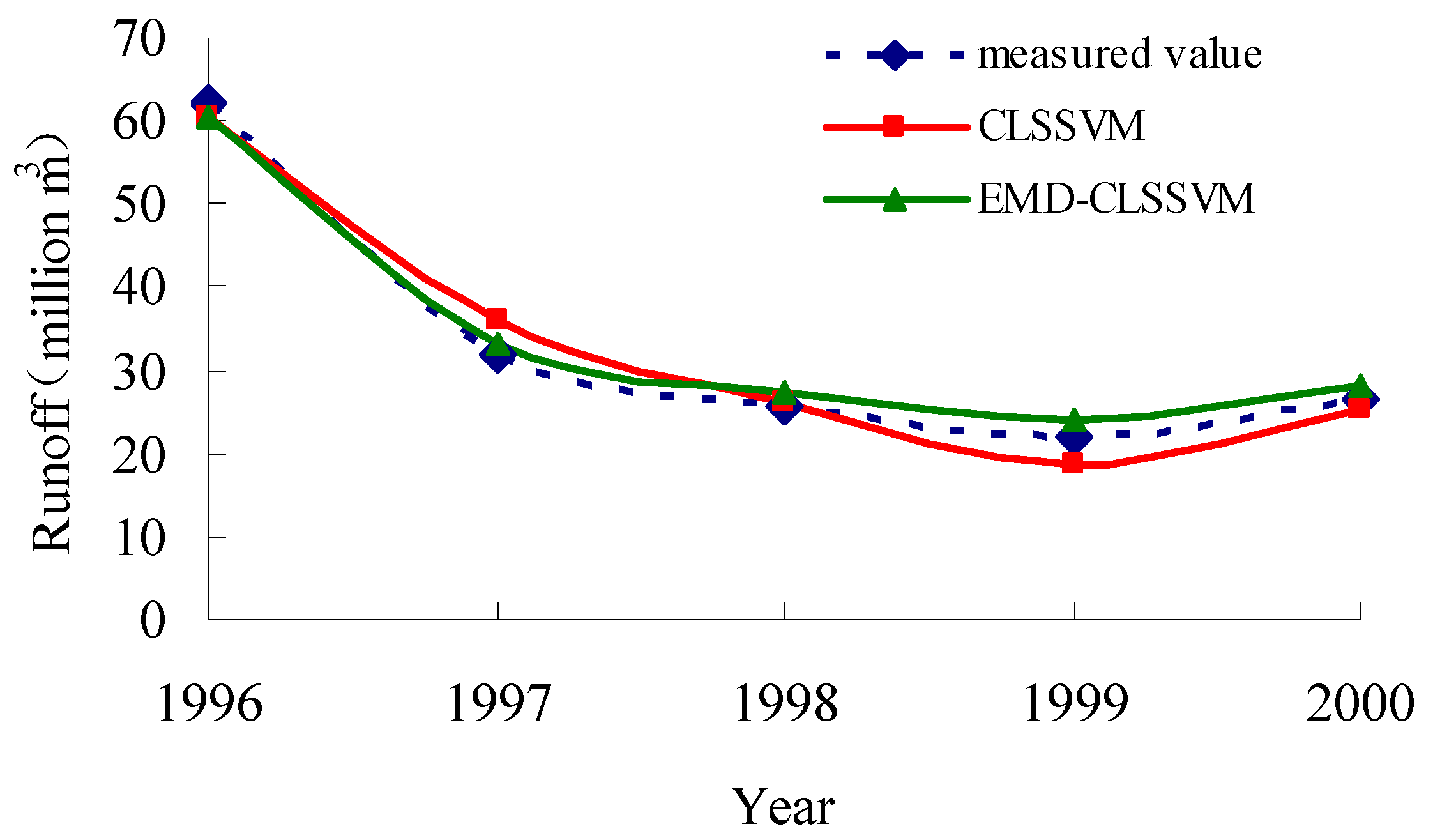
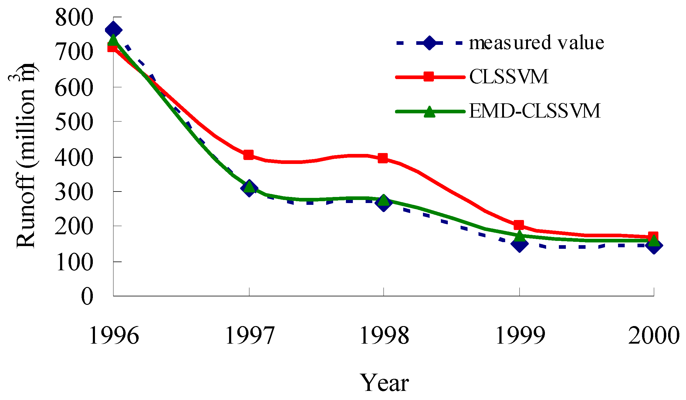
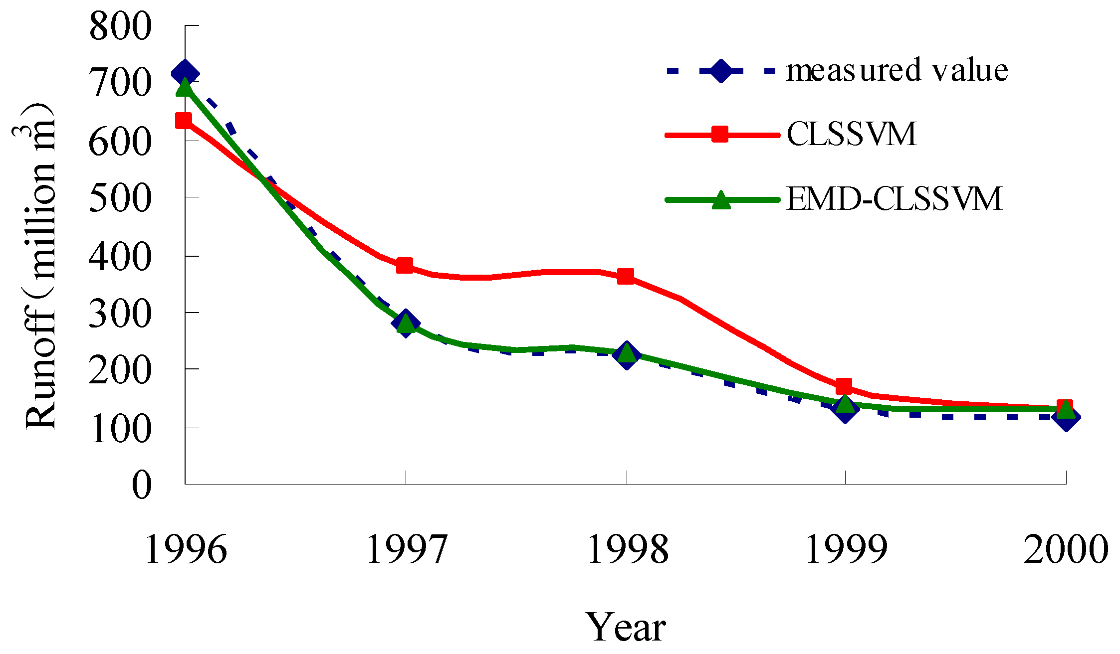
3.6. Comparative Analysis

To verify the stability and representativeness of the EMD-CLSSVM hybrid model, Fenhe reservoir, Zhaishang, and Lancun stations are used as examples. The original runoff series are decomposed into several IMFs and a trend term is based on the EMD for the three hydrologic stations, as shown in Figure 6, Figure 7 and Figure 8.

Analysis results of the chaotic characteristics of runoff series for the three stations are given in

Table 3. LM statistic, delay time τ, embedding dimension m, average period p, and Lyapunov exponent λ₁ of IMFs for the three stations.

Stations	IMFs	LM Statistic	τ	m	Average Period p	Lyapunov Exponent λ1
Fenhe reservoir	IMF1	0.180	1	7	7	0.091
	IMF2	0.087	1	7	7	0.042
	IMF3	0.105	3	6	6	0.023
	IMF4	0.112	3	5	5	0.168
	IMF5	0.363	2	4	23	—
Zhaishang	IMF1	0.248	1	7	7	0.01
	IMF2	0.119	2	7	7	0.169
	IMF3	0.097	2	3	3	0.169
	IMF4	0.335	1	4	23	—
Lancun	IMF1	0.129	1	7	7	0.163
	IMF2	0.129	2	7	7	0.017
	IMF3	0.082	2	4	4	0.140
	IMF4	0.329	2	4	23	—

.

Similarly, it can be seen in Table 3 that the Lyapunov exponent λ₁ of the IMFs for Fenhe reservoir, Zhaishang, and Lancun stations are more than 0, except for the IMF5 for Fenhe reservoir station and the IMF4 for Zhaishang and Lancun stations, which indicates that the IMFs have chaotic characteristics. The average period of the IMF5 for Fenhe reservoir station and the IMF4 for Zhaishang and Lancun stations is 23 years. Therefore, the Power Spectrum method is used to analyze the chaotic characteristics of the IMF5 for Fenhe reservoir station, and the IMF4 for Zhaishang and Lancun stations. Figure 9, Figure 10 and Figure 11 show that the IMF5 for Fenhe reservoir stations and the IMF4 for Zhaishang and Lancun stations each have single peaks, which indicates that the three time series do not have chaotic characteristics.

The prediction results analyzed from Figure 12, Figure 13 and Figure 14 are similar to those in Figure 5. It can be seen from the hydrographs that the CLSSVM hybrid model shows worse performance for annual runoff forecasting than the EMD-CLSSVM hybrid model in the testing period, especially in Figure 13 and Figure 14.

3.7. Evaluation of Model Performance

To evaluate the performance of the models, qualified rate (QR), root mean square errors (RMSE), mean absolute relative errors (MARE), and mean absolute errors (MAE) are employed to measure the goodness of fit of various models in this paper. Each statistical measure provides unique insight into the performance of the model. The forecast value is eligible if the forecast relative error is less than 20% [31]. The QR is defined as the ratio of the number of eligible years to the number of prediction years. Model performance can be measured as “satisfactory” if QR > 70%, as “good” if QR > 80%, as “very good” if QR > 90%, and as “unsatisfactory” if QR < 70%. RMSE and MARE provide different types of information about the predictive capabilities of the model. MAE provides a more balanced measure of goodness of fit at moderate values [32].

The assessments of training and testing results obtained by the two models for four stations are presented in

Table 4. Performance indicators of different models for four hydrologic stations during training and testing periods.

Station	Hybrid Model	Training				Testing
		QR	RMSE (106 m3)	MARE	MAE (106 m3)	QR	RMSE (106 m3)	MARE	MAE (106 m3)
Shangjingyou	CLSSVM	61%	10.19	0.21	8.12	100%	2.49	0.07	2.03
	EMD-CLSSVM	97%	3.78	0.07	2.93	100%	1.52	0.05	1.51
Fenhe reservoir	CLSSVM	65%	120.33	0.27	70.83	100%	11.03	0.05	9.89
	EMD-CLSSVM	97%	75.17	0.21	53.43	100%	9.93	0.03	7.95
Zhaishang	CLSSVM	68%	114.91	0.32	90.91	40%	77.05	0.26	67.64
	EMD-CLSSVM	97%	40.19	0.09	30.33	100%	17.71	0.07	15.72
Lancun	CLSSVM	58%	106.63	0.30	65.58	40%	85.84	0.30	74.17
	EMD-CLSSVM	97%	24.18	0.07	19.11	100%	12.16	0.05	10.18

Note: QR: qualified rate; RMSE: root mean square errors; MARE: mean absolute relative errors; MAE: mean absolute errors.

.

Table 4 shows that the EMD-CLSSVM hybrid model for Shangjingyou station has good performance during both training and testing. In the training period, the EMD-CLSSVM hybrid model obtained good QR, RMSE, MARE and MAE statistics, which increases the QR by 59%, and reduces the RMSE, MARE, and MAE by 62.9%, 66.7%, and 63.9%, respectively, in comparison with CLSSVM hybrid model. The EMD-CLSSVM hybrid model obtained good QR, RMSE, MARE, and MAE statistics in the testing period, reducing the RMSE, MARE, and MAE by 39%, 28.6%, and 25.6%, respectively, in comparison with the CLSSVM hybrid model.

Table 4 shows that the performance of the CLSSVM hybrid model is worse than the EMD-CLSSVM hybrid model for the other three hydrologic stations. Training QR and testing QR of the EMD-CLSSVM hybrid model for the other three hydrologic stations also reach up to 97% and 100%, respectively. The training QR of the CLSSVM hybrid model for the other three hydrologic stations is about 60%, and the testing QR of the CLSSVM hybrid model for Fenhe reservoir station is 100%. However, the testing QR of the CLSSVM hybrid model for Zhaishang and Lancun stations is 40%, i.e., it is disqualified. It can be observed from Table 4 that EMD significantly increases the accuracy of the CLSSVM hybrid model in terms of RMSE, MARE, and MAE. For Fenhe reservoir station in the training period, the EMD-CLSSVM hybrid model reduces the RMSE, MARE, and MAE by 37.5%, 22.2%, and 24.6%, respectively, as comparison with the CLSSVM hybrid model. In the testing period, the reductions in RMSE, MARE, and MAE are 10%, 40%, and 19.6%, respectively. For Zhaishang station in the training period, the EMD-CLSSVM hybrid model reduces the RMSE, MARE and MAE by 65%, 71.9%, and 66.6%, respectively, in comparison with the CLSSVM hybrid model. In the testing period the reductions in the RMSE, MARE, and MAE are 77%, 73.1%, and 76.8%, respectively. For Lancun station in the training period, the EMD-CLSSVM hybrid model reduces the RMSE, MARE, and MAE by 77.3%, 76.7%, and 70.9%, respectively, in comparison with the CLSSVM hybrid model. In the testing period the reductions in the RMSE, MARE, and MAE are 85.8%, 83.3%, and 86.3%, respectively. Similarly, it can be seen from Table 4 that the EMD-CLSSVM hybrid model has better accuracy in forecasting annual runoff at Fenhe reservoir, Zhaishang, and Lancun stations, which is consistent with the results for Shangjinyou station. Therefore, the forecasting results of the other three stations have further confirmed the high consistency and good stability of the EMD-CLSSVM hybrid model.

The optimal model that gives the minimum RMSE, MARE, and MAE was selected. The EMD-CLSSVM hybrid model has good performance with lower RMSE, MARE, and MAE values. The reason the forecasting accuracy of the EMD-CLSSVM hybrid model is better than that of the CLSSVM hybrid model lies in the advantages of EMD, e.g., decomposing the original runoff series into several sub-series and transforming the time series into stationary ones. A stationary series is needed when selecting the parameters of phase space in chaotic theory. A nonstationary time series affects the performance of phase space reconstruction, which leads to a reduction in prediction accuracy. In practice, it is very difficult to forecast nonstationary annual runoff series. EMD is introduced to transform nonstationary series into stationary ones, taking advantage of a combination of chaotic theory and LSSVM methods, which enhances the prediction accuracy. On the other hand, EMD is also a decomposition process. The decomposition strategy does effectively enhance the prediction accuracy. From Table 4, it is clear that the prediction accuracy of the CLSSVM hybrid model is worse than the prediction accuracy of the EMD-CLSSVM hybrid model. For example, compared to the CLSSVM hybrid model, the RMSE, MARE, and MAE of the EMD-CLSSVM hybrid model are all reduced by more than 80% for Lancun station in the testing period; the RMSE, MARE, and MAE of the EMD-CLSSVM hybrid model are reduced by more than 70% for Zhaishang station in the testing period. Zhaishang station and Lancun station are located in the lower reaches of the Fenhe reservoir. The runoff time series are affected by human activities at the two stations, including the characteristics of multi-scale changes. These results indicate that many multi-scale components with different characteristics exist in the runoff time series. The decomposition process segregates the multi-scale components from the runoff time series and predicts the components separately, and this can enhance the forecasting performance.

The main reason for this improvement is that the EMD-CLSSVM hybrid model is capable of decomposing original runoff series into stationary time series using EMD, which indicates that the EMD-CLSSVM hybrid model significantly outperformed the CLSSVM hybrid model. The models applied to the four hydrological stations have achieved consistent results, which indicates that the EMD-CLSSVM hybrid model has the characteristics of high consistency and great stability.

4. Conclusions

If the runoff series possesses a chaotic trait, the traditional forecasting methods cannot perform properly. To improve the accuracy of runoff forecasting, the LSSVM model may be an effective tool for the prediction of chaotic runoff series. Thus, the EMD-CLSSVM hybrid model was investigated for prediction purpose. The EMD-CLSSVM hybrid model was coupled with the EMD technique, chaotic theory, LSSVM, and other forecasting methods. The annual runoff data from Shangjingyou station in Lan River, a tributary of the Fenhe River in China, were used to develop the model, while Fenhe reservoir, Zhaishang, and Lancun in Fenhe River in China were used to verify the proposed method. Firstly, the KPSS method was used to analyze the stationarity of the runoff series. The results showed that the runoff series for four hydrologic stations was nonstationary. Using the EMD technique, the original runoff series were decomposed into several IMFs and one trend term. After the KPSS test, it was found that the decomposed IMFs were stationary. On this basis, the chaotic theory was employed to analyze the chaotic characteristics of several IMFs. It is indicated that the IMF1, IMF2, IMF3, and IMF4 for Shangjingyou and Zhaishang stations have chaotic characteristics. So do the IMF1, IMF2, and IMF3 for Zhaishang and Lancun stations. The remaining IMFs have no chaotic characteristics. Then the CLSSVM model was used to predict the IMF1, IMF2, IMF3, and IMF4 for Shangjingyou and Zhaishang stations, and the IMF1, IMF2, and IMF3 for Zhaishang and Lancun stations; the polynomial method was employed to predict the last IMF, and the GM was applied to predict the trend term. Finally, the prediction result was reconstructed to obtain the prediction value of the original runoff series. The results showed that the EMD-CLSSVM hybrid model has good performance in comparison with the CLSSVM hybrid model. For four hydrological stations, the EMD-CLSSVM hybrid model increased QR with respect to the CLSSVM hybrid model by 30%–60% and reduced RMSE, MARE, and MAE by 10%–85.8%, 22.2%–83.3%, and 19.6%–86.3%, respectively. Although runoff generation is impacted by many factors, no exogenous variables are considered in this paper. The reason is that a chaotic runoff series carries enough information about the behavior of the system to carry out forecasting. Moreover, this paper focuses on the advantages of the proposed method. However, directly applying the CLSSVM hybrid model for runoff prediction does not produce a better result. The reason is that a nonstationary runoff series limits prediction accuracy. Therefore, the EMD has been introduced for stationarity conduct of the runoff series. The method proposed in this paper can be applied to the remaining reaches of Fenhe River, where data are available. It would also have potential application in other catchments with a similar environment.

References

1. Yaseen, Z.M.; El-Shafie, A.; Jaafar, O.; Afan, H.A.; Sayl, M.N. Artificial intelligence based models for stream-flow forecasting: 2000–2015. J. Hydrol. 2015, 530, 829–844. [Google Scholar] [CrossRef]
2. Kisi, O.; Nia, A.M.; Goshen, M.G.; Tajabadi, M.R.J.; Ahmadi, A. Intermittent streamflow forecasting by using several data driven techniques. Water Resour. Manag. 2012, 26, 457–474. [Google Scholar] [CrossRef]
3. Barge, J.T.; Sharif, H.O. An ensemble empirical mode decomposition, self-organizing map, and linear genetic programming approach for forecasting River streamflow. Water 2016, 8, 247. [Google Scholar] [CrossRef]
4. Chang, J.X.; Zhang, H.X.; Wang, Y.M.; Zhu, Y.L. Assessing the impact of climate variability and human activities on streamflow variation. Hydrol. Earth Syst. Sci. 2016, 20, 1547–1560. [Google Scholar] [CrossRef]
5. Chen, C.S.; Liu, C.H.; Su, H.C. A nonlinear time series analysis using two-stage genetic algorithms for streamflow forecasting. Hydrol. Process. 2008, 22, 3697–3711. [Google Scholar] [CrossRef]
6. Chiew, F.H.S.; Potter, N.J.; Vaze, J.; Petheram, C.; Zhang, L.; Teng, J.; Post, D.A. Observed hydrologic non-stationarity in far south-eastern Australia: Implications for modelling and prediction. Stoch. Environ. Res. Risk Assess. 2014, 28, 3–15. [Google Scholar] [CrossRef]
7. Islam, M.N.; Sivakumar, B. Characterization and prediction of runoff dynamics: A nonlinear dynamical view. Adv. Water Resour. 2002, 25, 179–190. [Google Scholar] [CrossRef]
8. Hu, Z.Y.; Zhang, C.; Luo, G.P.; Teng, Z.D.; Jia, C.J. Characterizing cross-scale chaotic behaviors of the runoff time series in an inland river of Central Asia. Quat. Int. 2013, 311, 132–139. [Google Scholar] [CrossRef]
9. Dhanya, C.T.; Kumar, D.N. Predictive uncertainty of chaotic daily streamflow using ensemble wavelet networks approach. Water Resour. Res. 2011, 47. [Google Scholar] [CrossRef]
10. Sivakumar, B.; Bemdtsson, R.; Persson, M. Monthly runoff prediction using phase space reconstruction. Hydrol. Sci. J. 2001, 46, 377–387. [Google Scholar] [CrossRef]
11. Tongal, H. Nonlinear forecasting of stream flows using a chaotic approach and artificial neural networks. Earth Sci. Res. J. 2013, 17, 119–126. [Google Scholar]
12. Fathima, T.A.; Jothiprakash, V. Behavioural analysis of a time series—A chaotic approach. Sadhana-Acad. Proc. Eng. Sci. 2014, 39, 659–676. [Google Scholar] [CrossRef]
13. Liu, Q.; Islam, S.; Rodriguez-lturbe, I.; Le, Y. Phase-space analysis of daily streamflow: Characterization and prediction. Adv. Water Resour. 1998, 21, 463–475. [Google Scholar] [CrossRef]
14. Zhang, Q.; Wang, B.D.; He, B.; Peng, Y.; Ren, M.L. Singular spectrum analysis and ARIMA hybrid model for annual runoff forecasting. Water Resour. Manag. 2011, 25, 2683–2703. [Google Scholar] [CrossRef]
15. Karthikeyan, L.; Kumar, D.N. Predictability of nonstationary time series using wavelet and EMD based ARMA models. J. Hydrol. 2013, 502, 103–119. [Google Scholar] [CrossRef]
16. Kisi, O.; Latifoglu, L.; Latifoglu, F. Investigation of empirical mode decomposition in forecasting of hydrological time series. Water Resour. Manag. 2014, 28, 4045–4057. [Google Scholar] [CrossRef]
17. Huang, S.Z.; Chang, J.X.; Huang, Q.; Chen, Y.T. Monthly streamflow prediction using modified EMD-based support vector machine. J. Hydrol. 2014, 511, 764–775. [Google Scholar] [CrossRef]
18. Di, C.L.; Yang, X.H.; Wang, X.C. A four-stage hybrid model for hydrological time series forecasting. PLoS ONE 2014, 9. [Google Scholar] [CrossRef] [PubMed]
19. Mwale, F.D.; Adeloye, A.J.; Rustum, R. Application of self-organising maps and multi-layer perceptron-artificial neural networks for streamflow and water level forecasting in data-poor catchments: The case of the Lower Shire floodplain, Malawi. Hydrol. Res. 2014, 45, 838–854. [Google Scholar] [CrossRef]
20. Alvaro, L.R.; Vicente, L.F.; David, P.V.; Joaquin, T.P. One-Day-Ahead Streamflow forecasting using artificial neural networks and a meteorological mesoscale model. J. Hydrol. Eng. 2015, 20, 05015001. [Google Scholar]
21. Liu, Z.Y.; Zhou, P.; Chen, G.; Guo, L.D. Evaluating a coupled discrete wavelet transform and support vector regression for daily and monthly streamflow forecasting. J. Hydrol. 2014, 519, 2822–2831. [Google Scholar] [CrossRef]
22. Sudheer, C.; Maheswaran, R.; Panigrahi, B.; Mathur, S. A hybrid SVM-PSO model for forecasting monthly streamflow. Neural Comput. Appl. 2014, 24, 1381–1389. [Google Scholar] [CrossRef]
23. Shabri, A.; Suhartono, S. Streamflow forecasting using least-squares support vector machines. Hydrol. Sci. J. 2012, 57, 1275–1293. [Google Scholar] [CrossRef]
24. Samsudin, R.; Saad, P.; Shabri, A. River flow time series using least squares support vector machines. Hydrol. Earth Syst. Sci. 2011, 15, 1835–1852. [Google Scholar] [CrossRef] [Green Version]
25. Huang, N.E.; Shen, Z.; Long, S.R.; Wu, M.L.C.; Shih, H.H.; Zheng, Q.N.; Yen, N.C.; Tung, C.C.; Liu, H.H. The empirical mode decomposition and the Hilbert spectrum for nonlinear and non-stationary time series analysis. Proc. R. Soc. Lond. A 1998, 454, 903–995. [Google Scholar] [CrossRef]
26. Fraser, A.M.; Swinney, H.L. Independent coordinates for strange attractors from mutual information. Phys. Rev. A 1986, 33, 1134–1140. [Google Scholar] [CrossRef]
27. Kugiumtzis, D. State space reconstruction parameters in the analysis of chaotic time series—The role of the time window length. Phys. D 1996, 95, 13–28. [Google Scholar] [CrossRef]
28. Cao, L.Y. Practical method for determining the minimum embedding dimension of a scalar time series. Phys. D 1997, 110, 43–50. [Google Scholar] [CrossRef]
29. Kwiatkowski, D.; Phillips, P.C.B.; Schmidt, P.; Shin, Y.C. Testing the null hypothesis of stationarity against the alternative of a unit-root-How sure are we that economic time series have a unit-root? J. Econometr. 1992, 54, 159–178. [Google Scholar] [CrossRef]
30. Vallejos, R.O.; Anteneodo, C. Theoretical estimates for the largest lyapunov exponent of many-particle systems. Phys. Rev. E 2002, 66. [Google Scholar] [CrossRef] [PubMed]
31. Ministry of Water Resources. SL250–2000, Standard for Hydrological Information and Hydrological Forecasting; China Water and Power Press: Beijing, China, 2000.
32. Karunanithi, N.; Grenney, W.J.; Whitley, D.; Bovee, K. Neural networks for river flow prediction. J. Comput. Civ. Eng. ASCE 1994, 8, 201–220. [Google Scholar] [CrossRef]
Figure 1. Locations of four hydrologic stations in the Fenhe River basin of China.
Water 09 00153 g001
Figure 2. Empirical mode decomposition (EMD) results of runoff series for Shangjingyou station.
Water 09 00153 g002
Figure 3. Delay time τ of several intrinsic mode functions (IMFs) for Shangjingyou station ((a) IMF1; (b) IMF2; (c) IMF3; (d) IMF4; and (e) IMF5).
Water 09 00153 g003aWater 09 00153 g003b
Figure 4. Power spectrum of IMF5 for Shangjingyou station.
Water 09 00153 g004
Figure 5. Prediction results of annual runoff for Shangjingyou station. CLSSVM: chaotic least squares support vector machine; EMD-CLSSVM: EMD-based chaotic LSSVM.
Water 09 00153 g005
Figure 6. EMD results of runoff series for Fenhe reservoir station.
Water 09 00153 g006
Figure 7. EMD results of runoff series for Zhaishang station.
Water 09 00153 g007
Figure 8. EMD results of runoff series for Lancun station.
Water 09 00153 g008
Figure 9. Power spectrum of IMF5 for Fenhe reservoir station.
Water 09 00153 g009
Figure 10. Power spectrum of IMF4 for Zhaishang station.
Water 09 00153 g010
Figure 11. Power spectrum of IMF4 for Lancun station.
Water 09 00153 g011
Figure 12. Prediction results of annual runoff for Fenhe reservoir station.
Water 09 00153 g012
Figure 13. Prediction results of annual runoff for Zhaishang station.
Water 09 00153 g013
Figure 14. Prediction results of annual runoff for Lancun station.
Water 09 00153 g014