Temporal Downscaling of Crop Coefficients for Winter Wheat in the North China Plain: A Case Study at the Gucheng Agro-Meteorological Experimental Station

Abstract

The crop coefficient (K_c) is widely used for operational estimation of actual evapotranspiration (ET_a) and crop water requirements. The standard method for obtaining K_c is via a lookup table from FAO-56 (Food and Agriculture Organization of the United Nations Irrigation and Drainage Paper No. 56), which broadly treats K_c as a function of four crop-growing stages. However, the distinctive physiological characteristics of overwintering crops, such as winter wheat (Triticum aestivum L.), which is extensively planted in the North China Plain (NCP), are not addressed in this method. In this study, we propose a stage-wise method that accounts for K_c variations for winter wheat at each critical phenological stage, thereby estimating K_c at finer temporal scales. Compared with the conventional FAO method, the proposed stage-wise method successfully captures the bimodal pattern in K_c time series for winter wheat, which is shown at both ten-day and phenological time scales. In addition, the accuracies of the proposed stage-wise K_c method and the FAO method were evaluated using micro-meteorological measurements of ET_a collected at the Gucheng agro-meteorological experimental station in the NCP. Using a leave-one-out strategy, the evaluation revealed that the stage-wise method significantly outperformed the FAO method at both daily and critical phenological time scales, with root-mean-square errors in ET_a for the stage-wise method and the FAO method being 0.07 mm·day⁻¹ and 0.16 mm·day⁻¹, respectively, at the daily time scale, and 0.01 mm·day⁻¹ and 0.27 mm·day⁻¹ at the critical phenological time scale. Generally, the FAO method underestimates ET_a during the initial stage and overestimates ET_a during both the development and mid-season stages. It is shown that the proposed stage-wise method is important for the water-stressed NCP where precision irrigation is highly desirable, especially during the critical phenological stages. Results from this study provide insight into accurate estimation of water requirements for winter wheat at phenological time scales.

1. Introduction

The crop coefficient (K_c) is a crucial parameter that is widely applied in agricultural water management and irrigation scheduling, as it reflects the impacts of inherent crop biological characteristics and planting conditions on water requirements. K_c is defined as the ratio of crop evapotranspiration under well-watered conditions (ET_c) to a reference crop evapotranspiration (ET₀). ET_c is the evapotranspiration expected from disease-free, well-fertilized crops grown in large fields, under optimum soil water conditions and achieving full production under the given climatic conditions [1]. ET₀ is the evapotranspiration rate expected from a reference surface, which is hypothesized as a grass reference crop with specific characteristics limited only by atmospheric demand [1], considering only a constraint from the available energy.

Current approaches for estimating crop coefficients can be classified into two categories. The first category is based on the lookup table recommended by the Food and Agriculture Organization of the United Nations (the FAO method), including its related versions, which impose adjustments according to local climatic conditions, soil types, irrigation and crop management [2]. The second category involves separate estimation of ET_c and ET₀ via direct measurement or modeling. Methods for estimating ET_c include water balance assessments using weighing lysimeters [3,4,5,6,7] or soil water measurements [3,8], energy-conservation approaches using the Bowen ratio [9,10], eddy covariance techniques [11,12,13,14,15,16,17] or remote sensing retrievals (based on one-source [18] and two-source energy balance models) [19,20,21]. Methods for modeling ET₀ can be roughly divided into three categories [22,23], i.e., temperature models [24,25], radiation-temperature models [26,27] and combination models [1,28].

Among these, the FAO method is most popular given its simplicity and limited demands on data and processing steps. The FAO approach considers the crop coefficient as a function of four crop-growing stages, namely the initial, development, mid-season and late-season stages. However, the inherent biological characteristics of crops in different climatic zones are not considered in the FAO method. Specifically, for overwintering crops with dual peaks in their growth curves, the rapid growth stage before the overwintering period is smoothed or missed in the “four-stage” FAO method.

This distinctive phenological feature of overwintering crops has been confirmed in recent studies on the temporal downscaling of crop coefficients for winter wheat and other related crops, using both in situ measurements and soil water balance models. For example, studies investigating monthly K_c of winter wheat in Yangling of Shaanxi Province in China [3] and weekly K_c of rice-wheat rotation crops grown in the Indo-Gangetic plains of India [29] have all demonstrated the above-mentioned bimodal features in winter wheat. Generally, investigations on crop coefficients for winter wheat have been focusing on a particular growth stage, such as the post-elongation stage [30], the elongation to heading stage [31] and the green-up to ripening stage [32]. In contrast, research on K_c estimation covering the entire crop growth period from seedling emergence to the mature stage, as well as at multiple temporal scales (i.e., from the phenological stage scale to the ten-day fine scale) is rarely seen.

The North China Plain (NCP) region, regarded as the ‘Granary of China’, is characterized by water-intensive agricultural production with dominant cropping systems of winter wheat and summer maize rotation. Since precipitation during the winter wheat growing period is highly insufficient to meet water requirements, agricultural production in the NCP heavily relies on effective irrigation schemes, which require accurate information on ET_a and K_c.

As previously stated, for FAO methods, the inaccuracy in determining K_c of overwintering crops can cause non-negligible errors in estimated actual evapotranspiration (ET_a) during different phenological stages. To alleviate this problem, in this study, we propose a stage-wise method to temporally downscale K_c. The proposed K_c method makes full use of meteorological and eddy covariance data collected at the Gucheng agro-meteorological experimental station, maintained by the Chinese Academy of Meteorological Sciences (CAMS). The performances of the proposed K_c method and the conventional FAO method at both daily and phenological scales are evaluated against eddy covariance measurements of latent heat flux. The paper is organized as follows. Section 2 describes the establishment of the proposed stage-wise K_c model and the required datasets, including meteorological observations, eddy covariance measurements and soil moisture datasets. Section 3 reports the temporal dynamics of ET₀ and ET_a utilized for K_c estimation, and the K_c dynamics at different timescales including: (i) the “four-stage” scale (the same temporal scale used in the FAO method); (ii) critical phenological stages and (iii) the ten-day scale. The performance of the proposed method and the standard FAO method is assessed in comparison with surface flux measurements using a leave-one-year-out cross-validation method.

2. Methodology and Materials

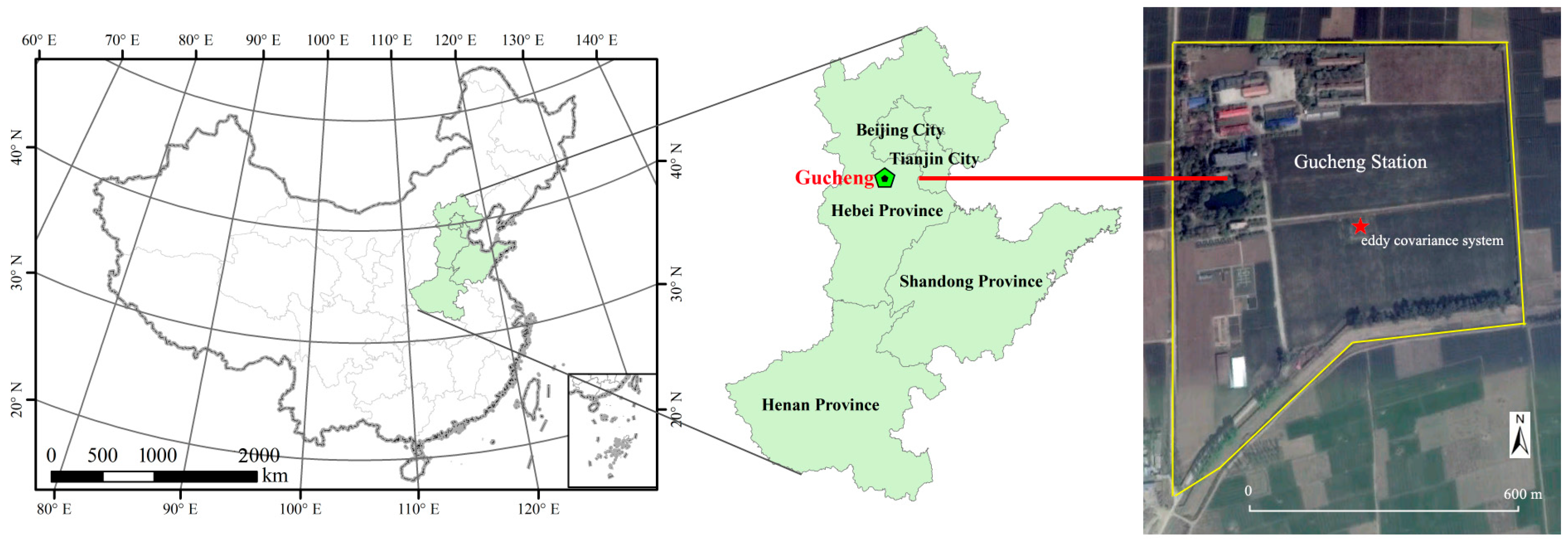
2.1. Gucheng Agro-Meteorological Experimental Station

Gucheng station is located in Hebei Province of the NCP region (115.73° E, 39.15° N, 15.2 m above mean sea level) and includes an area of approximately 150,000 m² (Figure 1). The station is in a temperate continental monsoon climate zone with mean annual precipitation of 474.9 mm, about 65%–85% of which is concentrated from June to September [33]. The meteorological records from 1997 to 2013 show an annual mean temperature of 12.0 °C and sunshine duration of 2158.8 h·year⁻¹. The dominant soil type at Gucheng station is a neutral loam, with a gentle slope and a deep arable soil layer. The station represents a high-yielding agricultural zone for winter wheat production in the NCP region, with relevant agro-meteorological variables extensively monitored in this experimental station.

2.2. Methodology

2.2.1. Reference Crop Evapotranspiration (ET₀) Estimation

The reference crop evapotranspiration, ET₀ (mm·day⁻¹), is estimated in this study using the FAO Penman–Monteith method [1]:

$$E{T}_0=\frac{0.408\times \Delta \left(R_{\mathrm{n}}-G\right)+\gamma ·\frac{900}{T+273}·U_2·\left(e_{\mathrm{s}}-e_{\mathrm{a}}\right)}{\Delta +\gamma ·\left(1+0.34U_2\right)}$$

(1)

where R_n is the net radiation (MJ·m⁻²·day⁻¹) and G is the soil heat flux (MJ·m⁻²·day⁻¹), which is assumed to be approximately 0 at the daily time scale. T is the average air temperature at a 2-m height (°C). U₂ is the average wind velocity at a 2-m height (m·s⁻¹). e_s and e_a are the saturated water vapor pressure and actual vapor pressure (kPa), respectively. Δ is the slope of the saturation vapor pressure curves (kPa·°C⁻¹). γ is the psychrometric constant (kPa·°C⁻¹).

Solar radiation was calculated with the Ångström–Prescott formula using extraterrestrial radiation and relative sunshine duration [1]:

$$R_{\mathrm{s}}=\left(a_{\mathrm{s}}+b_{\mathrm{s}}\times \frac{n}{N}\right)\times R_{\mathrm{a}}$$

(2)

where R_s is the solar or shortwave radiation (MJ·m⁻²·day⁻¹) and R_a is the extraterrestrial radiation (MJ·m⁻²·day⁻¹). N is the maximum possible duration of sunshine or daylight hours (hour), n is the actual duration of sunshine (hour), and n/N is the relative sunshine duration. The parameters a_s and b_s are Ångström values (dimensionless), which vary with location and time of year. In this study, both a_s and b_s are adopted following Mao et al. [34].

2.2.2. Estimation of Crop Evapotranspiration under Standard Conditions (ET_c)

With proper management within the footprint of the flux tower at Gucheng station, there was sufficient supply of water and nutrition for the winter wheat crop and no pest or disease damage. Therefore, the actual evapotranspiration ET_a can be considered as well-watered ET_c. In this study, the ET_a was acquired by two approaches: (1) direct measurements from the eddy covariance (EC) system, and (2) indirect estimation using the water balance equation. Tower-based ET_a measurements collected during the growing season in a two-year study period are used to establish a crop coefficient model for winter wheat, and the estimated K_c is validated using a leave-one-year-out cross-validation (LOOCV) method. Meanwhile, the ET_a derived from an independent approach based on water balance equation is also used to evaluate K_c for winter wheat. The details for deriving ET_a from the two approaches are described in the following two subsections.

ET_a Calculated Using Eddy Flux Measurements

Daily latent heat flux was accumulated from half-hour data collected with the EC system and was then converted to ET_a using the latent heat of water vaporization:

$$E{T}_{\mathrm{a}}=\frac{{{\displaystyle \sum }}_{i=1}^n\left(L{E}_i·t\right)}{\lambda ·\rho }$$

(3)

where ET_a is the daily actual evapotranspiration (mm·day⁻¹), LE_i is the half-hour latent heat flux (W·m⁻²), t is the time interval of sampling (1800 s), λ is the latent heat of water vaporization (2.44 MJ·kg⁻¹), ρ is the density of water (kg·m⁻³) and n is number of daily samples. The flux tower measurements and energy closure assessments are described further in Section 2.3.2.

ET_a Calculated by Water Balance Equation

The ET_a can also be calculated using a water balance equation in the following form:

$$\left(P+I+Q_{\mathrm{g}}\right)-\left(E{T}_{\mathrm{a}}+R+D\right)=\Delta W_{\mathrm{s}}+\Delta W_{\mathrm{v}}$$

(4)

where P is the precipitation (mm), I is the irrigation (mm), Q_g is the contribution from the water table (mm), ET_a is the actual evapotranspiration (mm), R is the surface runoff (mm) and D is the deep drainage (mm). The left-hand side of Equation (4) is the water budget during the study period, while ΔW_s and ΔW_v are the water content variations (mm) during the same period for soil and canopy, respectively.

As the topography of the experimental site is relatively flat and the precipitation is not intensive during the growing period of winter wheat (annual average precipitation is about 138.7 mm during the study period), the surface runoff and the deep drainage can be neglected in this case [8,11,35,36]. Contributions from groundwater are also negligible as the water table is over 30 m deep. As the canopy equivalent water thickness (EWT) of winter wheat during the entire growing period is less than 1 mm [37], the water content variations of crop (ΔW_v) can be neglected. Thus, the ET_a based on the water balance equation can be expressed as:

$$E{T}_{\mathrm{a}}=\left(P+I\right)-\Delta W_{\mathrm{s}}=\left(P+I\right)-\left({\theta }_{\mathrm{v}1}-{\theta }_{\mathrm{v}2}\right)$$

(5)

where θ_v1 and θ_v2 are the volumetric soil water contents measured with time domain reflectometry (TDR, TRIME^®-TDR-PICO-IPH/T3, Imko, Ettlingen, Germany) at the beginning and end of the study period, respectively.

2.2.3. Crop Coefficient (K_c) Estimation

In this paper, the effects of both crop transpiration and soil evaporation on ET_a were integrated into the single parameter of K_c. The K_c of a specific crop reflects the crop characteristics and its climatic features, i.e., changes in vegetation are reflected in K_c variations during the growing period. As stated in the Section 1, the standard FAO method is employed in the study as a reference to benchmark the proposed stage-wise K_c method. Both methods are introduced in detail in the following subsections.

Proposed Stage-Wise Method

The crop coefficient of winter wheat during each phenological period (Equation (6)) was estimated using the temporally-averaged reference crop evapotranspiration ET₀ (Equation (1)) and the measured crop evapotranspiration under standard conditions ET_c (represented by ET_a):

$$K_{\mathrm{c},i}=E{T}_{\mathrm{c},i}/E{T}_{0,i}$$

(6)

where the subscript i denotes the different phenological periods of interest. K_c,i > 1 indicates that ET_c,i is higher than ET_0,i, which usually occurs during the rapid growing stage; while K_c,i < 1 is generally observed during the initial growing stage, when the plant height and leaf area index are low.

In this study, K_c calculated by the water balance equation using TDR soil moisture measurement is referred to as K_c_TDR, so as to distinguish it from the K_c calculated using eddy fluxes, denoted as K_c_Eddy.

The FAO Method

In the FAO method, K_c is considered as a function of crop growth stages, namely the initial, development, mid-season and late-season stages. Only three values are required to construct the K_c curve: K_c during the initial stage (K_c,ini), the mid-season stage (K_c,mid) and the late-season stage (K_c,end). According to the lookup table for single crop coefficients under the FAO method [1], typical values of K_c,ini, K_c,mid and K_c,end for winter wheat with frozen soils are taken as 0.40, 1.15 and 0.25–0.40. At Gucheng station in the NCP region, winter wheat is harvested shortly after ripening; therefore, a high value of 0.40 is used for K_c,end. As for the K_c,mid, the effect of aerodynamic properties is not only crop-specific, but also depends on the climatic conditions and crop height. Thus, K_c,mid can be adjusted based on the meteorological observations as below [1]:

$$K_{\mathrm{c},\mathrm{mid}}=K_{\mathrm{c},\mathrm{mid}\left(\mathrm{tab}\right)}+\left[0.04\times \left(U_2-2\right)-0.004\times \left(R{H}_{\min }-45\right)\right]\times {\left(h/3\right)}^{0.3}$$

(7)

where K_c,mid(tab) is the typical value of K_c,mid listed in the FAO handbook. U₂, RH_min and h are the mean values for daily wind speed at a 2-m height (m·s⁻¹), daily minimum relative humidity (%) and plant height (m) during the mid-season stage. After adjustment, K_c,mid is 1.15 at Gucheng station, the same as the typical value for crop coefficients of winter wheat during the mid-season stage in the FAO method.

2.2.4. Leave-One-Year-Out Cross-Validation

Cross-validation [38] is a model validation technique for assessing how the results of statistical analysis will generalize to an independent dataset. When there is not enough data to partition into separate training and validating sets without losing significant modeling or validation capability, cross-validation provides an effective means to evaluate model performance.

Leave-one-year-out cross-validation (LOOCV) [39] involves using one year of observations as the validation set and observations from the remaining years as the training set. This is repeated n times (n is the number of observation years in the original sample) to partition the original sample into training and validation sets.

2.3. Materials

2.3.1. Meteorological Observations

The meteorological data used in the computation of ET₀, including daily average air temperature, maximum air temperature, minimum air temperature, vapor pressure, atmospheric pressure, relative humidity, wind speed and sunshine duration, were collected from an automatic weather station in Gucheng during 2009–2014. All observations were quality controlled and contained no missing records during the study period.

2.3.2. Eddy Covariance Measurements

The eddy covariance system was installed at a height of 4 m above the ground level on a flux tower in the eastern part of Gucheng station, and winter wheat was planted in the tower fetch of up to 500 m in the prevailing wind direction. The system consists of a sonic anemometer and CO₂/H₂O analyzer, sampling fluxes of sensible heat, latent heat and CO₂ at a high frequency of 10 Hz, with data stored in the data logger at both 10 Hz and half-hour intervals. Additional instruments include a four-component net radiometer and a soil heat flux plate buried under the soil surface at a 5-cm depth.

Previous studies showed that the performance of coordinate rotation can be omitted as the corresponding errors were less than 1% at Gucheng station due to flat terrain [40]. Additionally, these studies demonstrated that half-hour is an acceptable interval for averaging the high-frequency flux observations obtained from the height below 30-m level [40,41,42,43]. Meanwhile, the 30-min averaging period is commonly used by the micro-meteorological community for flux measurements over agricultural sites [14,15]. Thus, in this study, the 30-min EC data we used were processed from the original high-frequency observations after a series of processing steps, including spike removal, WPL (Webb, Pearman, and Leuning) correction, sonic virtual temperature correction and frequency response correction. In addition, quality control was performed to minimize the effects of extreme weather conditions and equipment malfunction on the flux data. Specifically, the obvious outliers in the time series and invalid nocturnal measurements taken with friction velocity <0.08 m·s⁻¹ were excluded [44]. Following this, the missing data for small gaps (2–3 half-hourly missing) were replaced by linear interpolation using the adjacent value(s) [45], whereas large data gaps were filled using exponential regression equations [46] developed for each individual stage, namely the seedling growth stage, dormancy stage and rapid growth stage. To avoid inaccurate interpolation, days with continuous data gaps exceeding 1/3 of the daily record length, resulting from either missing measurements or quality control, were completely removed during model construction and validation. After these treatments, two years with reliable flux observations, i.e., the winter wheat growing periods for 2009–2010 and 2012–2013 (denoted as the study periods of 2009 and 2012 hereinafter), were included in the analysis.

The typical energy closure condition in the EC measurements was evaluated for each phenological stage of the two-year study period using the energy balance ratio (EBR) [47]. EBR < 100% indicates that the measurements do not fully characterize the local flux conditions, with errors typically attributed to the underestimation of sensible and latent fluxes and/or the overestimation of available energy during nocturnal periods, especially weak turbulent periods [48]. Closure ratios of 80% or higher are considered to be reasonable at most sites with climate zones ranging from Mediterranean to temperate and arctic [48].

2.3.3. Soil Water Content Measurements

Soil water content was measured by TDR once every 10 days (i.e., on the 8th, 18th and 28th days of each month) during the growing period of winter wheat for 2013 and 2014. According to ground measurements in the southern NCP region, the mean of total root length density (RLD) for winter wheat is 57.7% from surface down to a 0.5 m depth, and the value is 81.1% from surface down to 1.0 m [49]. Therefore, in this study, soil moisture was measured at 0.1 m intervals from the surface down to a 1.0 m depth to account for the change of soil water content within the root zone. The soil moisture was recorded in percentage units (%) with an accuracy of ±4% according to instrument manual.

2.3.4. Remotely Sensed Leaf Area Index (LAI) Time Series

The Moderate Resolution Imaging Spectroradiometer (MODIS) 8-day LAI product (MOD15A2, https://reverb.echo.nasa.gov/reverb/) at 1-km spatial resolution during the winter wheat growing season from two years (2009 and 2012) was used to indirectly evaluate the K_c estimation, as temporal dynamics of LAI and K_c have proven to be highly correlated [3]. The time series of MODIS LAI in the pixel collocated with Gucheng station during the two-year study period was extracted, and the QC flags were used to exclude unreliable observations, retaining data retrieved by the main retrieval method. Consequently, a linear interpolation method was used to construct a complete 8-day time series of LAI and, finally, re-sampled at a ten-day interval so as to be consistent with K_c at the temporal scale.

2.3.5. Meteorological Conditions during the Winter Wheat Growing Period

The winter wheat used in this experiment was a medium-early maturing variety. The detailed growing conditions for each winter wheat variety, including growing dates and field management, during the two-year study period are listed in

Table 1. Winter wheat varieties and meteorological conditions at Gucheng station during the growing seasons of the two-year study period.

Year	Variety	Seeding Date MM/DD	Ripening Date MM/DD	Average Temperature (°C)	Average Maximum Temperature (°C)	Average Minimum Temperature (°C)
2009–2010	Jimai-22	10/10	6/20	5.9	11.7	0.6
2012–2013	Jimai-22	10/08	6/19	5.8	12.4	0.4

. For the two-year study period, the average temperature, average maximum temperature and average minimum temperature were 5.9 °C, 12.1 °C and 0.5 °C, respectively, with little inter-annual variation during the winter wheat growing period (Table 1). Total precipitations were 125.5 mm and 193.8 mm, which temporally coincide with the dry season. The percentages of rainy days occupied 17.4% and 12.8% for the two growing seasons respectively, and flood irrigations were applied 4–5 times for each growing season. On average, water supply throughout the growing periods was generally regulated by weekly rainfall and/or irrigation. Therefore, precipitation has little constraining impact on winter wheat growth and, thus, is excluded from the discussion in this paper.

3. Results and Discussion

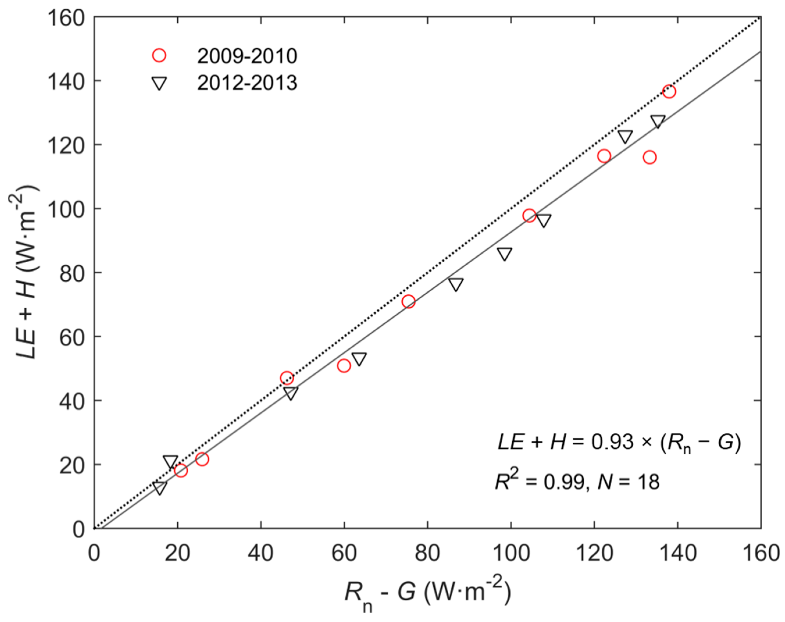
3.1. Energy Balance Closure of Flux Measurements

A scatter plot comparing the surface fluxes (LE + H) and the available energy (R_n −G) measured at the flux tower during all critical phenological stages is shown in Figure 2. The EBRs for the two growing periods range from 90.39% to 91.35%. The mean EBRs for the seedling, dormancy and rapid-growth periods are 94.14%, 84.83% and 91.58%, respectively, all higher than the mean EBR of 80% for a diverse range of vegetation covers and climate types [48]. The good closure conditions observed in Figure 2 indicate that the ET_a measurements used to compute K_c_Eddy are reasonable.

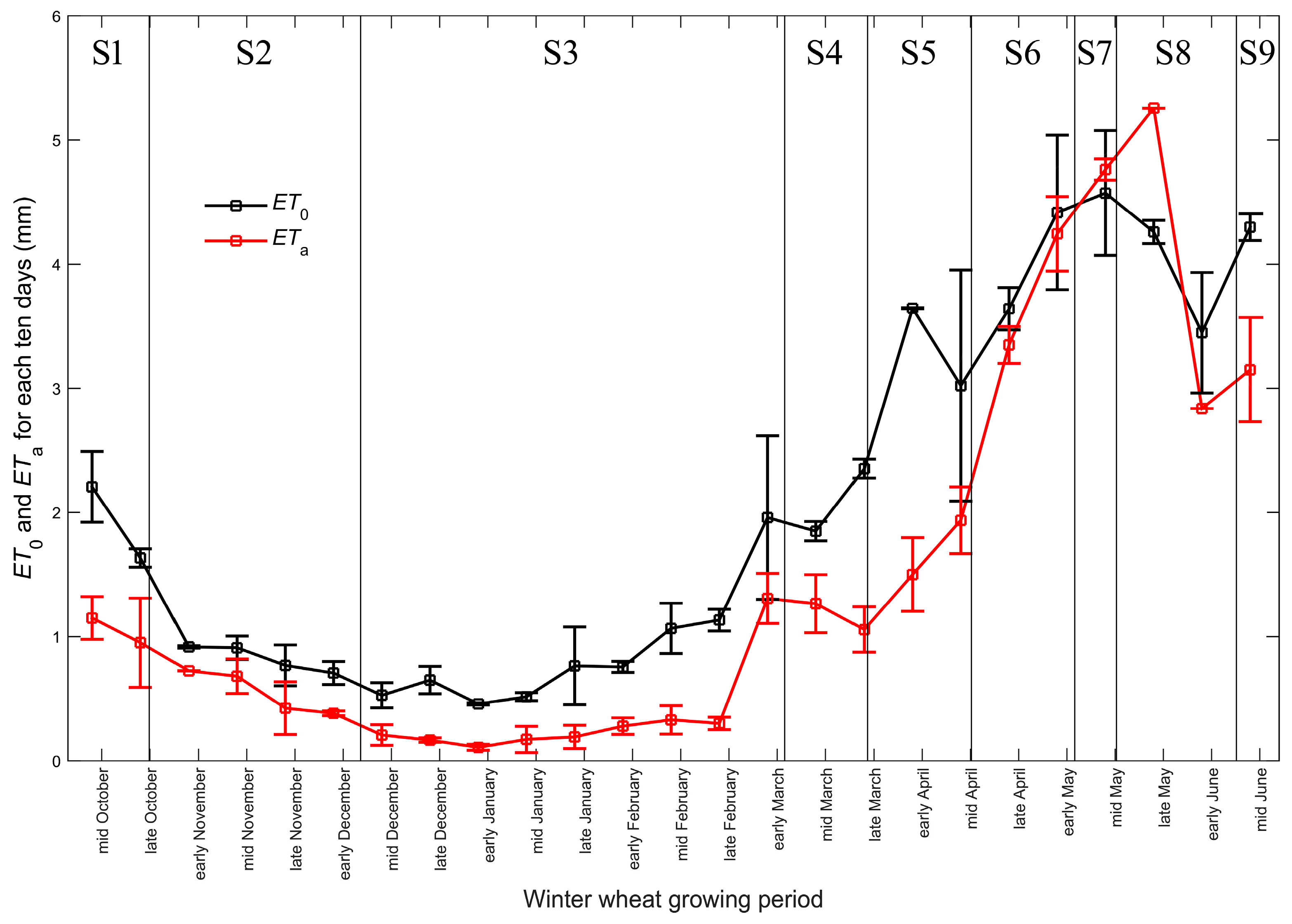
3.2. ET₀ and ET_a Dynamics

Temporal dynamics of ET₀ calculated using the FAO Penman–Monteith method and ET_a obtained from eddy covariance observations at Gucheng station during growing seasons are shown in Figure 3. These curves are computed on 10-day intervals and represent averages over the two-year study period. The vertical lines in Figure 3 represent the nine generalized growth stages (S1–S9) for winter wheat, as tabulated in

Table 2. The growing stages of winter wheat and its corresponding phenological periods according to the FAO method.

DOY	Phenological Stages	Stage-Wise Method	FAO Method
DOY284	Seeding	Stage 1	Initial stage
DOY290	Seedling emergence
DOY304	Three-leaf	Stage 2
DOY321	Tiller
DOY338	Stop growing	Stage 3
DOY062	Green-up	Stage 4
DOY088	Erect-growing	Stage 5	Development stage
DOY111	Elongation	Stage 6
DOY122	Booting	Stage 7	Mid-season stage
DOY130	Heading	Stage 8
DOY136	Blossom
DOY155	Milk	Stage 9	Late-season stage
DOY171	Ripening

.

In the early growth stages from seedling to green-up (S1–S4), both ET₀ and ET_a are low due to low insolation levels and low air temperature during fall to winter. Starting from the S4 stage, the rising temperatures and solar radiation have resulted in increasing ET₀ and ET_a. As the canopy starts to close during the erect-growing to blossom stages (S5–S8), ET_a approaches the potential rate. Both ET (ET₀ and ET_a) curves show the highest degree of inter-annual variability during S5–S8. In particular, the inter-annual variations of ET_a mainly occurred during the rapid growing periods, i.e., late March–early May, due to variability in crop canopy height, LAI and leaf morphology between years. ET_a downturn occurs in the milking to ripening stage (S9), as the green canopy covers begin to decline.

3.3. Estimated K_c at Three Different Temporal Scales

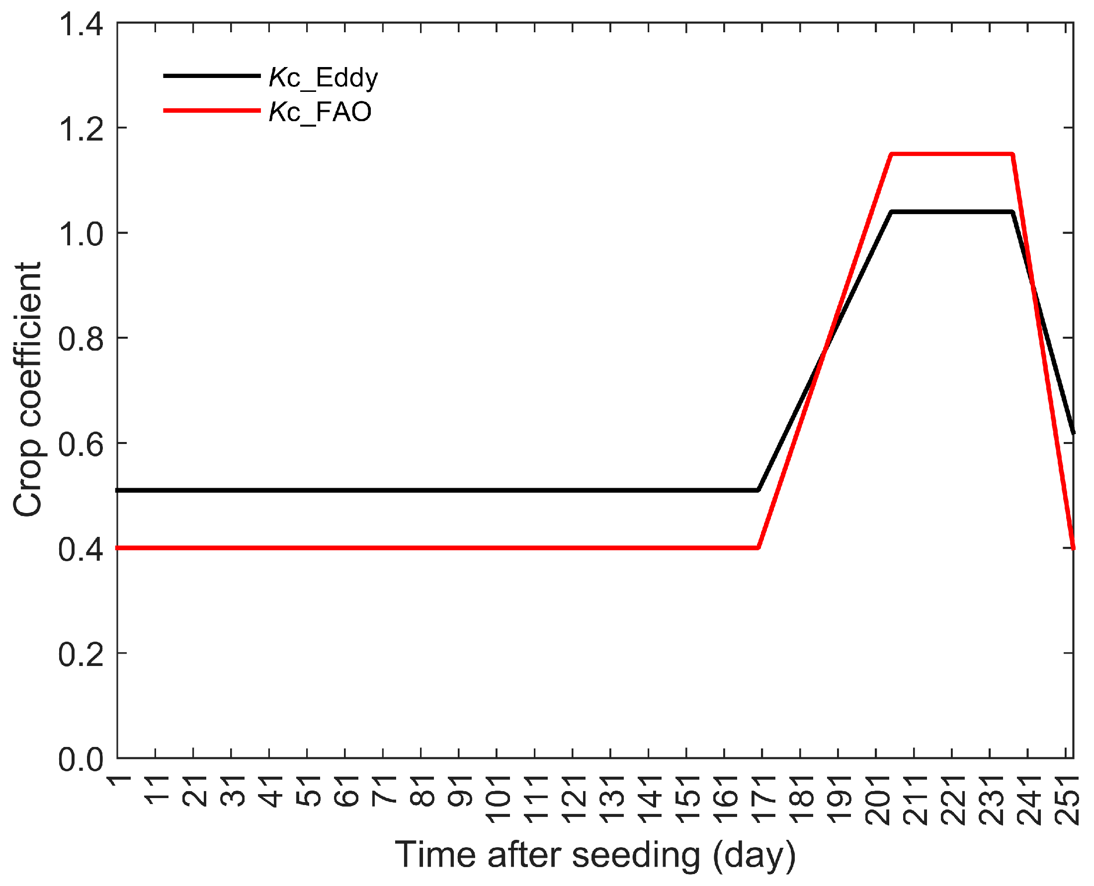
3.3.1. Comparison with the Four-Stage FAO Method

In order to directly compare the capabilities of characterizing winter wheat K_c between the proposed stage-wise methods and the “four-stage” FAO method, we regrouped the nine finer-scale phenological stages of winter wheat in our method to match the “four-stage” in the FAO method. Specifically, the initial stage in the FAO method corresponds to the seeding to green-up stages; the crop development stage and mid-season stage cover the erect to elongation stages and booting to blossom stages, respectively; and the late-season stage corresponds to the milk to harvest stages (Table 2).

Based on this regrouping scheme, K_c time series derived from both the FAO method (referred to as K_c_FAO) and the proposed stage-wise method (based on two years of quality-controlled eddy covariance fluxes (see Section 2.3.2), referred to as K_{c_}Eddy) are illustrated in Figure 4, showing noticeable differences between two sets of K_c values. In particular, K_{c_}Eddy exceeds K_c_FAO in the initial and late-season stage and is lower than K_c_FAO during the mid-season stage. This is mainly attributed to the difference in climatic features between the sub-humid region (where the FAO method was originally developed) and this study region in the NCP. Specifically, the FAO method for winter wheat K_c was originally developed for sub-humid regions with average daily minimum relative humidity (RH_min) around 45% and moderate wind speeds of 2 m·s⁻¹. However, meteorological conditions at Gucheng station are quite different, representing semi-arid and sub-humid climates with sparse rainfall during the winter wheat growing period. In addition, the average RH_min for the two-year study period was about 31.6%, well below the expected 45% that generated the typical K_c_FAO values.

As soil moisture is not a limiting factor for evapotranspiration with regard to the experimental design at the Gucheng site (which provides sufficient irrigation, as mentioned in Section 2.3.5), the relatively large atmospheric demand enhance the potential soil evaporation and crop transpiration, and therefore, increased ET_a, resulting in higher K_{c_}Eddy than K_c_FAO during the initial stage. Differences in K_c values during the mid-season stage may be attributed to lower crop heights at Gucheng station (0.7 m) in comparison with the expected maximum height of winter wheat in the FAO method (1.0 m). Since crop transpiration accounted for considerable portion of ET_a during the mid-season stage, the relatively shorter crop height at Gucheng may be responsible for the lower K_c_Eddy than K_c_FAO. As for the late-season stage, winter wheat at Gucheng station was harvested immediately after reaching mature stage, so as to prepare for the sowing of second crop-rotation (maize). Therefore, K_c_Eddy of winter wheat at Gucheng station for the late-season stage was significantly higher than K_c_FAO before ET_a dropped to the minimum value. It is worth noting that due to the prevailing maize-wheat rotation system in NCP, this common agricultural practice of immediate harvesting of winter wheat after the mature stage is a human-induced factor that contributes to the unsuitability of the FAO method across this region.

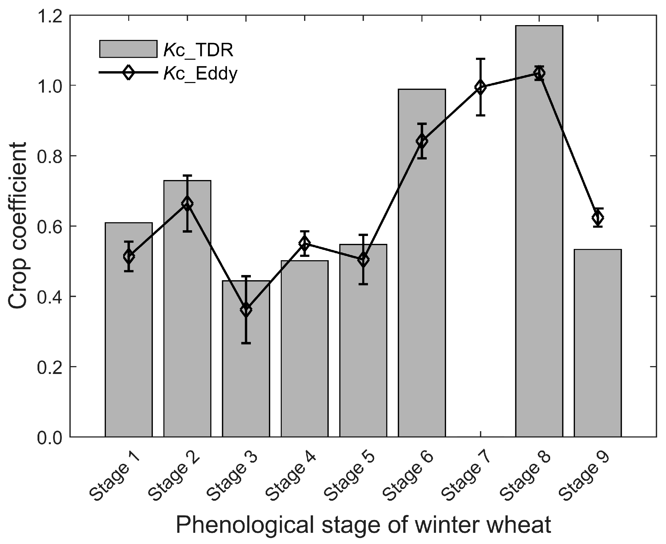
3.3.2. K_c Dynamics at the Critical Phenological Stages

To examine K_c dynamics at Gucheng station at finer temporal scales, K_c values for winter wheat developed using ET_a estimates from eddy covariance (K_c_Eddy) and water balance (K_c_TDR) are compared at the time scale of critical phenological stages in Figure 5.

As seen in Figure 5, the temporal dynamics of both K_c_Eddy and K_c_TDR exhibit similar bimodal features during the growing period. The winter wheat development cycle is characterized by two rapid growing periods, namely the three-leaf to dormancy stages and the erect-growing to booting stages, which occur before and after overwintering, respectively. This is similar to other studies of K_c features of winter wheat using both in situ observations [3] and models [50,51]. It is noted that due to the neglect of the rapid growing period before overwintering in the FAO method, the actual water consumption prior to the green-up stage was considerably underestimated by approximately 9 mm, accounting for 10.5% of actual water consumption during the initial stage.

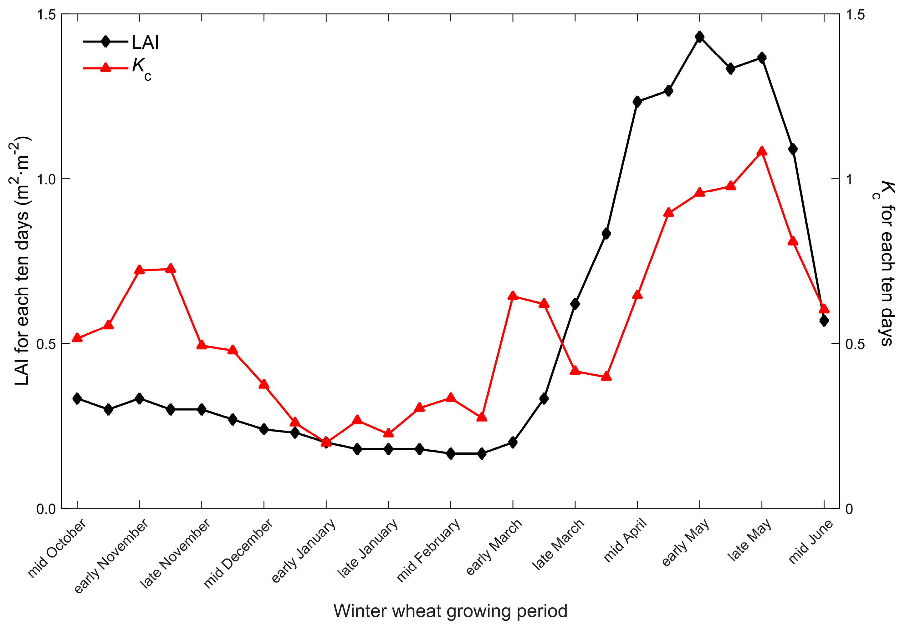
3.3.3. K_c Dynamics at the Ten-Day Scale

The average K_c_Eddy dynamics at Gucheng station are compared with that of LAI observations at the 10-day scale in Figure 6. Overall, the temporal dynamics of K_c and LAI at the 10-day scale were highly correlated as expected. Specifically, at this 10-day time scale, the two peaks in the K_c_Eddy curve from late November to early December and from mid-April to late May are very evident, as well as a clear overwintering feature. During the overwintering to erect-growing stages, i.e., from mid-December to the next mid-March, K_c_Eddy stayed at a low level and experienced little variability. Starting in March, K_c_Eddy increases significantly as the winter wheat starts rapid growth, with the main peak around mid-April at the booting stage. K_c_Eddy remains above 1.0, signifying high rates of water consumption until early June when winter wheat approached the mature stage.

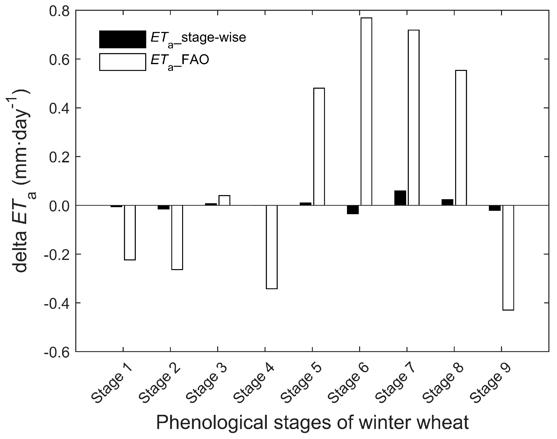
3.4. LOOCV of the Estimated ET_a Using the Proposed Stage-Wise Method

LOOCV was used to evaluate the performance of the stage-wise K_c method proposed in this study. The daily ET_a during the entire growing period estimated from the proposed stage-wise K_c method (K_c_Eddy) and the FAO method (K_c_FAO) is validated against measurements from the eddy covariance system at Gucheng station. The comparison statistics at both daily and critical phenological scales with the LOOCV technique are summarized in

Table 3. Statistical metrics of the comparison between the stage-wise and the FAO estimations of ET_a with the LOOCV method at the daily time scale.

Growing Period	Stage-Wise Method			FAO Method
	k *	R2	RMSE (mm·Day−1)	k *	R2	RMSE (mm·Day−1)
2009–2010	0.95	0.86	0.10	1.05	0.88	0.09
2012–2013	0.98	0.91	0.05	1.09	0.91	0.21
Sum-up	0.97	0.89	0.07	1.08	0.90	0.16

Note: * k is the regression coefficient with the linear equation “y = kx”.

and

Table 4. Statistical metrics of the comparison between the stage-wise and the FAO estimations of ET_a with the LOOCV method at the critical phenological time scale.

Growing Period	Stage-Wise Method			FAO Method
	k *	R2	RMSE (mm·Day−1)	k *	R2	RMSE (mm·Day−1)
2009–2010	0.99	0.96	0.03	1.07	0.92	0.20
2012–2013	1.00	0.95	0.01	1.13	0.96	0.34
Sum-up	1.00	0.96	0.01	1.09	0.93	0.27

Note: * k is the regression coefficient with the linear equation “y = kx”.

.

Generally, the proposed stage-wise method outperforms the FAO method in terms of linear regression coefficients k and root-mean-square errors (RMSEs). It is shown that the slope of the linear regression line (against ground measurements) for the stage-wise method is more approximate to unity compared to the FAO method (0.97 versus 1.08 at the daily scale and 1.00 versus 1.09 at the critical phenological scale). In addition, the outperformance of the stage-wise method over the FAO method is also supported by the metrics of RMSEs (0.07 mm·day⁻¹ versus 0.16 mm·day⁻¹ at the daily scale and 0.01 mm·day⁻¹ versus 0.27 mm·day⁻¹ at the critical phenological scale). In summary, our method showed slightly better performance than the FAO method in ET_a estimation during the growing period.

The errors in estimated ET_a for both the stage-wise and the FAO method at critical phenological stages are shown in Figure 7. From Figure 7, we can see that the uncertainties of ET_a from the stage-wise method are much smaller than those from the FAO method. Generally, during the initial stages, from seeding to the erect-growing stage, the ET_a derived from the FAO method is underestimated by −0.2 mm·day⁻¹, higher than that from the stage-wise method (−0.004 mm·day⁻¹). For the development stage and mid-season stage, the ET_a from the FAO method is notably overestimated by 0.63 mm·day⁻¹ and 0.64 mm·day⁻¹, which are higher than the overestimation from the stage-wise method (−0.01 mm·day⁻¹ and 0.04 mm·day⁻¹). The underestimations of ET_a in S9 are −0.02 mm·day⁻¹ and −0.43 mm·day⁻¹ from the stage-wise and FAO methods, respectively. Overall, a slight superiority of the proposed stage-wise method over the FAO method is exhibited for estimating actual evapotranspiration at phenological time scales.

4. Conclusions

The crop coefficient (K_c) is a crucial parameter in the estimation of actual water consumption and water requirement for agricultural development. In this study, a method to estimate temporal fine-scale K_c of winter wheat was developed using the meteorological and eddy covariance observations, as well as the winter wheat growing records during different phenological stages. This downscaling model is motivated by the significant bimodal feature in K_c time series of winter wheat and its distinctive overwintering characteristic, which are not addressed in the conventional FAO method.

Results show that compared to the “four-stage” FAO method, our proposed stage-wise method accurately captures the K_c peak before the overwintering stage and the trough during overwintering. In addition, our method can estimate K_c at temporally fine resolution at the crop development and mid-season stages and, thus, can serve as the basis for the accurate estimation of actual water consumption during the critical phenological stages of winter wheat.

The uncertainties in ET_a based on K_c derived from our proposed stage-wise method and the conventional FAO method are estimated during all critical phenological stages. Compared to the stage-wise method, the overestimation of ET_a from the FAO method is obvious with the maximum value of 0.77 mm·day⁻¹ during all of the critical phenological stages. The RMSEs of ET_a for the stage-wise and FAO methods are 0.07 mm·day⁻¹ and 0.16 mm·day⁻¹ at the daily scale and 0.01 mm·day⁻¹ and 0.27 mm·day⁻¹ at the critical phenological scale, respectively.

As Gucheng station represents a typical high-yield agricultural zone in the NCP region, the winter wheat K_c at the critical phenological stages generated from our method can be used as a reference for the entire NCP region, where in situ measurements of K_c are relatively scarce. However, accurate and spatially-distributed K_c at the crop phenological stages is crucial for precisely estimating crop water requirements, improving crop water use efficiency and yield, and consequently achieving the goal of highly-promoted water-saving irrigation. Further investigation on the spatial characteristics of winter wheat K_c at the phenological stages at the regional scale is needed. Meanwhile, the validation of the proposed framework in a larger observation sample is crucial in the future.

References

1. Allen, R.G.; Pereira, L.S.; Raes, D.; Smith, M. Crop Evapotranspiration: Guidelines for Computing Crop Water Requirements; FAO Irrigation & Drainage Paper 56; FAO: Rome, Italy, 1998. [Google Scholar]
2. Farg, E.; Arafat, S.M.; Abd EI-Wahed, M.S.; EL-Gindy, A.M. Estimation of Evapotranspiration ETc and Crop Coefficient Kc of Wheat, in south Nile Delta of Egypt Using integrated FAO-56 approach and remote sensing data. Egypt. J. Remote Sens. Space Sci. 2012, 15, 83–89. [Google Scholar] [CrossRef]
3. Kang, S.; Gu, B.; Du, T.; Zhang, J. Crop coefficient and ratio of transpiration to evapotranspiration of winter wheat and maize in a semi-humid region. Agric. Water Manag. 2003, 59, 239–254. [Google Scholar] [CrossRef]
4. Ko, J.; Piccinni, G.; Marek, T.; Howell, T. Determination of growth-stage-specific crop coefficients (Kc) of cotton and wheat. Agric. Water Manag. 2009, 96, 1691–1697. [Google Scholar] [CrossRef]
5. Abrisqueta, I.; Abrisqueta, J.M.; Tapia, L.M.; Munguía, J.P.; Conejero, W.; Vera, J.; Ruiz-Sánchez, M.C. Basal crop coefficients for early-season peach trees. Agric. Water Manag. 2013, 121, 158–163. [Google Scholar] [CrossRef]
6. Marsal, J.; Johnson, S.; Casadesus, J.; Lopez, G.; Girona, J.; Stöckle, C. Fraction of canopy intercepted radiation relates differently with crop coefficient depending on the season and the fruit tree species. Agric. For. Meteorol. 2014, 184, 1–11. [Google Scholar] [CrossRef]
7. Kumar, V.; Udeigwe, T.K.; Clawson, E.L.; Rohli, R.V.; Miller, D.K. Crop water use and stage-specific crop coefficients for irrigated cotton in the mid-south, United States. Agric. Water Manag. 2015, 156, 63–69. [Google Scholar] [CrossRef]
8. Gao, Y.; Duan, A.; Sun, J.; Li, F.; Liu, Z.; Liu, H.; Liu, Z. Crop coefficient and water-use efficiency of winter wheat/spring maize strip intercropping. Field Crops Res. 2009, 111, 65–73. [Google Scholar] [CrossRef]
9. Inmanbamber, N.G.; Mcglinchey, M.G. Crop coefficients and water-use estimates for sugarcane based on long-term Bowen ratio energy balance measurements. Field Crops Res. 2003, 83, 125–138. [Google Scholar] [CrossRef]
10. Hanson, B.R.; May, D.M. Crop coefficients for drip-irrigated processing tomato. Agric. Water Manag. 2006, 81, 381–399. [Google Scholar] [CrossRef]
11. Li, S.; Kang, S.; Li, F.; Zhang, L. Evapotranspiration and crop coefficient of spring maize with plastic mulch using eddy covariance in northwest China. Agric. Water Manag. 2008, 95, 1214–1222. [Google Scholar] [CrossRef]
12. Zhou, L.; Zhou, G. Measurement and modelling of evapotranspiration over a reed (Phragmites australis) marsh in Northeast China. J. Hydrol. 2009, 372, 41–47. [Google Scholar] [CrossRef]
13. Payero, J.O.; Irmak, S. Daily energy fluxes, evapotranspiration and crop coefficient of soybean. Agric. Water Manag. 2013, 129, 31–43. [Google Scholar] [CrossRef]
14. Facchi, A.; Gharsallah, O.; Corbari, C.; Masseroni, D.; Mancini, M.; Gandolfi, C. Determination of maize crop coefficients in humid climate regime using the eddy covariance technique. Agric. Water Manag. 2013, 130, 131–141. [Google Scholar] [CrossRef]
15. Liu, S.M.; Xu, Z.W.; Zhu, Z.L.; Jia, Z.Z.; Zhu, M.J. Measurements of evapotranspiration from eddy-covariance systems and large aperture scintillometers in the Hai River Basin, China. J. Hydrol. 2013, 487, 24–38. [Google Scholar]
16. Jiang, X.; Kang, S.; Tong, L.; Li, F.; Li, D.; Ding, R.; Qiu, R. Crop coefficient and evapotranspiration of grain maize modified by planting density in an arid region of northwest China. Agric. Water Manag. 2014, 142, 135–143. [Google Scholar] [CrossRef]
17. Zhang, H.; Anderson, R.G.; Wang, D. Satellite-based crop coefficient and regional water use estimates for Hawaiian sugarcane. Field Crops Res. 2015, 180, 143–154. [Google Scholar] [CrossRef]
18. Bastiaanssen, W.G.M.; Menenti, M.; Feddes, R.A.; Holtslag, A.A.M. A remote sensing surface energy balance algorithm for land (SEBAL). 1. Formulation. J. Hydrol. 1998, 212–213, 198–212. [Google Scholar] [CrossRef]
19. Norman, J.M.; Kustas, W.P.; Humes, K.S. A two-source approach for estimating soil and vegetation energy fluxes from observations of directional radiometric surface temperature. Agric. For. Meteorol. 1995, 77, 263–293. [Google Scholar] [CrossRef]
20. Anderson, M.C.; Norman, J.M.; Mecikalski, J.R.; Otikin, J.A.; Kustas, W.P. A climatological study of evapotranspiration and moisture stress across the continental United States based on thermal remote sensing: 2. Surface moisture climatology. J. Geophys. Res. Atmos. 2007, 112, 311–368. [Google Scholar] [CrossRef]
21. Sánchez, J.M.; López-Urrea, R.; Rubio, E.; González-Piqueras, J.; Vaselles, V. Assessing crop coefficients of sunflower and canola using two-source energy balance and thermal radiometry. Agric. Water Manag. 2014, 137, 23–29. [Google Scholar] [CrossRef]
22. McMahon, T.A.; Peel, M.C.; Lowe, L.; Srikanthan, R.; McVicar, T.R. Estimating actual, potential, reference crop and pan evaporation using standard meteorological data: A pragmatic synthesis. Hydrol. Earth Syst. Sci. 2013, 17, 1331–1363. [Google Scholar] [CrossRef]
23. McMahon, T.A.; Finlayson, B.L.; Peel, M.C. Historical developments of models for estimating evaporation using standard meteorological data. WIREs Water 2016, 3, 788–818. [Google Scholar] [CrossRef]
24. Thornthwaite, C.W. An approach toward a rational classification of climate. Geogr. Rev. 1948, 38, 55–94. [Google Scholar] [CrossRef]
25. Hargreaves, G.H.; Samani, Z.A. Reference crop evapotranspiration from temperature. Appl. Eng. Agric. 1985, 1, 96–99. [Google Scholar] [CrossRef]
26. Priestley, C.H.B.; Taylor, R.J. On the assessment of surface heat and evaporation using large scale parameters. Mon. Weather Rev. 1972, 100, 81–92. [Google Scholar] [CrossRef]
27. Tegos, A.; Malamos, N.; Koutsoyiannis, D. A parsimonious regional parametric evapotranspiration model based on a simplification of the Penman–Monteith formula. J. Hydrol. 2015, 524, 708–717. [Google Scholar] [CrossRef]
28. Monteith, J.L. Evaporation and environment. In The State and Movement of Water in Living Organisms; Fogg, G.E., Ed.; Cambridge University Press: London, UK, 1965; Volume 19, pp. 205–234. [Google Scholar]
29. Choudhury, B.U.; Singh, A.K.; Pradhan, S. Estimation of crop coefficients of dry-seeded irrigated rice–wheat rotation on raised beds by field water balance method in the Indo-Gangetic plains, India. Agric. Water Manag. 2013, 123, 20–31. [Google Scholar] [CrossRef]
30. Su, M.; Li, J.; Rao, M. Estimation of crop coefficients for sprinkler-irrigated winter wheat and sweet corn using a weighing lysimeter. Trans. Chin. Soc. Agric. Eng. 2005, 21, 25–29. [Google Scholar]
31. Liu, H.; Kang, Y. Calculation of crop coefficient of winter wheat at elongation-heading stages. Trans. Chin. Soc. Agric. Eng. 2006, 22, 52–56. [Google Scholar]
32. Li, H.L.; Luo, Y.; Zhao, C.J.; Yang, G.J. Estimating crop coefficients of winter wheat based on canopy spectral vegetation indices. Trans. Chin. Soc. Agric. Eng. 2013, 29, 118–127. [Google Scholar]
33. Zhang, H.; Feng, L.P. Characteristics of Spatio-temporal Variation of Precipitation in North China in Recent 50 Years. J. Nat. Resour. 2010, 25, 270–279. [Google Scholar]
34. Mao, F.; Zhao, Y.J.; Sun, H.; Shao, P.; Liao, S.H.; Jiang, H.F.; Zheng, X.B. Spatial and Temporal Change Characteristics of ÅngstrÖm-Prescott Coefficients in China in 1961–2010. Meteorol. Environ. Sci. 2016, 39, 43–51. [Google Scholar]
35. Silva, V.P.R.; Silva, B.B.; Albuquerque, W.G.; Borges, C.J.R.; Sousa, I.F.; Neto, J.D. Crop coefficient, water requirements, yield and water use efficiency of sugarcane growth in Brazil. Agric. Water Manag. 2013, 128, 102–109. [Google Scholar] [CrossRef]
36. Wang, Z.; Wu, P.; Zhao, X.; Gao, Y.; Chen, X. Water use and crop coefficient of the wheat-maize strip intercropping system for an arid region in northwestern China. Agric. Water Manag. 2015, 161, 77–85. [Google Scholar] [CrossRef]
37. Yilmaz, M.T.; Hunt, E.R.; Jackson, T.J. Remote sensing of vegetation water content from equivalent water thickness using satellite imagery. Remote Sens. Environ. 2008, 112, 2514–2522. [Google Scholar] [CrossRef]
38. Maatouk, H.; Roustant, O.; Richet, Y. Cross-Validation Estimations of Hyper-Parameters of Gaussian Processes with Inequality Constraints. Procedia Environ. Sci. 2015, 27, 38–44. [Google Scholar] [CrossRef]
39. Zhang, T. A leave-one-out cross validation bound for kernel methods with applications in learning. In Computational Learning Theory: Lecture Notes in Computer Science; Springer: Berlin/Heidelberg, Germany, 2001; pp. 427–443. [Google Scholar]
40. Guo, J.X. Characters and Parameterization Comparisons of Turbulent Transfer over Maize Field on North China Plain. Ph.D. Dissertation, Chinese Academy of Meteorological Sciences and Nanjing University of Information Science & Technology, Nanjing, China, 2006. [Google Scholar]
41. Berger, B.W.; Davis, K.J.; Yi, C.; Bakwin, P.S.; Zhao, C.L. Long-Term Carbon Dioxide Fluxes from a Very Tall Tower in a Northern Forest: Flux Measurement Methodology. J. Atmos. Ocean. Technol. 2001, 18, 529–542. [Google Scholar] [CrossRef]
42. Zhang, P.; Yuan, G.F.; Zhu, Z.L. Determination of the average period of Eddy covariance measurement and its influences on the calculation of fluxes in desert riparian forest. Arid Land Geogr. 2013, 36, 400–408. [Google Scholar]
43. Liu, Y.J.; Hu, F.; Cheng, X.L.; Feng, Y.F. Data processing and quality assessment of the eddy covariance system of the 325-meter meteorology tower in Beijing. Chin. J. Atmos. Sci. 2016, 40, 390–400. (In Chinese) [Google Scholar]
44. Zhu, Z.L.; Sun, X.M.; Wen, X.F.; Zhou, Y.L.; Tian, J.; Yuan, G.F. Study on the processing method of nighttime CO2 eddy covariance flux data in China FLUX. Sci. China Earth Sci. 2006, 49, 36–46. [Google Scholar] [CrossRef]
45. Falge, E.; Baldocchi, D.; Olson, R.; Anthoni, P.; Aubinet, M.; Bernhofer, C.; Burba, G.; Ceulemans, R.; Clement, R.; Dolman, H.; et al. Gap filling strategies for defensible annual sums of net ecosystem exchange. Agric. For. Meteorol. 2001, 107, 43–69. [Google Scholar] [CrossRef]
46. Zhou, L.; Zhou, G.; Liu, S.; Sui, X. Seasonal contribution and interannual variation of evapotranspiration over a reed marsh (Phragmites australis) in Northeast China from 3-year eddy covariance data (pages 1039–1047). Hydrol. Process. 2010, 24, 1039–1047. [Google Scholar] [CrossRef]
47. Gu, J.; Smith, E.A.; Merritt, J.D. Testing energy balance closure with GOES-retrieved net radiation and in situ measured eddy correlation fluxes in BOREAS. J. Geophys. Res. Atmos. 1999, 104, 27881–27894. [Google Scholar] [CrossRef]
48. Wilson, K.; Goldstein, A.; Falge, E.; Aubinet, M.; Baldocchi, D.; Berbigier, P.; Bernhofer, C.; Ceulemans, R.; Dolman, H.; Field, C.; et al. Energy balance closure at FLUXNET sites. Agric. For. Meteorol. 2002, 113, 223–243. [Google Scholar] [CrossRef]
49. Liu, R.H.; Zhu, Z.X.; Fang, W.S.; Deng, T.H.; Zhao, G.Q. Distribution pattern of winter wheat root system. Chin. J. Ecol. 2008. [Google Scholar] [CrossRef]
50. Liu, Y.; Teixeira, J.L.; Zhang, H.J.; Pereira, L.S. Model validation and crop coefficients for irrigation scheduling in the North China plain. Agric. Water Manag. 1998, 36, 233–246. [Google Scholar] [CrossRef]
51. Parkes, M.; Wang, J.; Knowles, R. Peak crop coefficient values for Shaanxi, North-west China. Agric. Water Manag. 2005, 73, 149–168. [Google Scholar] [CrossRef]
Figure 1. Location of the Gucheng agro-meteorological station in the North China Plain (NCP) region of China (the extent of the station is outlined in yellow line in the rightmost sub-figure).
Water 09 00155 g001
Figure 2. Energy balance closure during all critical phenological stages of winter wheat in two-year study period at Gucheng station.
Water 09 00155 g002
Figure 3. ET0 and ETa for winter wheat at 10-day intervals during the growing period averaged over the two-year study period. The error bars show the standard deviation in ET0 and ETa for each interval over the two years. Vertical lines indicate nine generalized growth stages (S1–S9) for winter wheat.
Water 09 00155 g003
Figure 4. Comparison of Kc between the proposed stage-wise method and the FAO method.
Water 09 00155 g004
Figure 5. The proposed stage-wise Kc during the critical phenological stages.
Water 09 00155 g005
Figure 6. Ten-day Kc_Eddy and LAI from 2-year average (2009 and 2012).
Water 09 00155 g006
Figure 7. Comparison of delta ETa for winter wheat between the stage-wise method and the FAO method during the critical phenological stages.
Water 09 00155 g007