Article

Groundwater Modeling and Sustainability of a Transboundary Hardrock–Alluvium Aquifer in North Oman Mountains

1
Water Research Center, Sultan Qaboos University, Muscat 123, Oman
2
Department of Hydroinformatics, East Water and Environmental Research Institute, Mashhad 9176873384, Iran
*
Author to whom correspondence should be addressed.
Water 2017, 9(3), 161; https://doi.org/10.3390/w9030161
Submission received: 8 December 2016 / Revised: 16 February 2017 / Accepted: 20 February 2017 / Published: 24 February 2017

Abstract

:
This study aims at modeling groundwater flow using MODFLOW in a transboundary hardrock–alluvium aquifer, located in northwestern Oman. A three-dimensional stratigraphic model of the study area representing the vertical and spatial extent of four principal hydro-geologic units (specifically, the Hawasina, ophiolite, Tertiary and alluvium) was generated using data collected from hundreds drilled borehole logs. Layer elevations and materials for four layers grid cells were taken from the generated stratigraphic model in which the materials and elevations were inherited from the stratigraphic model that encompasses the cell. This process led to accurate grid so that the developed groundwater conceptual model was mapped to simulate the groundwater flow and to estimate groundwater balance components and sustainable groundwater extraction for the October 1996 to September 2013 period. Results show that the long-term lateral groundwater flux ranging from 4.23 to 11.69 Mm3/year, with an average of 5.67 Mm3/year, drains from the fractured eastern ophiolite mountains into the alluvial zone. Moreover, the long-term regional groundwater sustainable groundwater extraction is 18.09 Mm3/year for 17 years, while it is, respectively, estimated as 14.51, 16.31, and 36.00 Mm3/year for dry, normal, and wet climate periods based on standardized precipitation index (SPI) climate condition. Considering a total difference in groundwater levels between eastern and western points of the study area on the order of 228 m and a 12-year monthly calibration period (October 1996 to September 2008), a root mean squared error (RMSE) in predicted groundwater elevation of 2.71 m is considered reasonable for the study area characterized by remarkable geological and hydrogeological diversity. A quantitative assessment of the groundwater balance components and particularly sustainable groundwater extraction for the different hydrological period would help decision makers to better understand the water resources in the Al-Buraimi region. In addition, it would assist decision makers to improve existing strategies to enhance the decision making for future developments.

1. Introduction

It is widely recognized that water will be one of the most important environmental concerns of this century [1]. As global populations and economies continue to increase exponentially, and as environmental change threatens the quantity and quality of water resources, attention has recently focused on the management of those waters which cross international boundaries [1,2,3,4,5].
Transboundary aquifers have long been recognized (e.g., [2,6]). However, their significance and function in environmental and human development has not enjoyed sufficient attention from policy makers, in contrast to transboundary surface water basins [3]. This is because surface water is more visible and exploited than groundwater; and its transboundary nature is often all too apparent when national boundaries are defined by streams or lakes. However, with critical attention on groundwater resources, especially during times of drought, there is more interest in the nature and extent of transboundary groundwater resources for better management [4].
Modeling is an important component of transboundary groundwater management systems. The use of numerical modeling to simulate groundwater behavior can enhance understanding of transboundary aquifer conditions and resources availability (e.g., [7,8,9,10,11,12,13,14,15,16,17,18,19,20,21,22,23]). Fendek and Fendekova [5] presented a numerical model to calculate available groundwater in the Zohor depression—an aquifer transcending national boundaries between the Slovak Republic and Austria. Rainwater et al. [8] described some of the scientific and non-technical pitfalls modelers can encounter in a transboundary modeling effort, using a model encompassing 21 counties in Texas. Weinthal et al. [10] discussed the Mediterranean Coastal Aquifer, shared by Israel and the Palestinian Authority, and described how overexploitation in the Gaza Strip has caused water table declines and water quality degradation. Siegfried and Kinzelbach [12] developed a simulation-optimization model for the northwest Sahara aquifer system which is being used non-cooperatively as a resource by Algeria, Tunisia, and Libya. Katic [13] adopted a hydro-economic model to estimate the size of the payoffs from the divergence between competitive and optimal rates of extraction from transboundary aquifers under alternative spatial representations. Milman and Ray [16] pointed out how uncertainty undermines collaborative transboundary groundwater management for the Santa Cruz aquifer, spanning the United States–Mexico border between Arizona and Sonora. They also discussed how data requirements and ambiguous interpretations exacerbate these uncertainties. Öztan and Axelrod [17] addressed how enhanced Turkey–Syria cooperation could impact management of the Ceylanpinar aquifer, which flows beneath both countries. They developed a simplified conceptual model to simulate water flow in the aquifer and showed how political changes may impact aquifer sustainability. Voss et al. [20] used GRACE satellite data to evaluate freshwater storage trends in the north-central Middle East, including portions of the Tigris and Euphrates river basins and western Iran. Sefelnasr et al. [23] developed a 3D GIS-based groundwater flow model for the Nubian Sandstone Aquifer System (NASA) to simulate the groundwater management options for the different development areas/oases within the aquifer.
Groundwater in the border regions of Sultanate of Oman and the United Arab Emirates (UAE) is an important resource for sustainable agricultural and urban developments for both countries. While the North Oman Mountains (NOMs), located at the east part of the study area, have been largely delineated as the principal recharge resources, there is no prior quantitative analysis of groundwater flow simulation for this transboundary aquifer. Therefore, the main objective of this study is to simulate groundwater behavior in the transboundary hardrock–alluvium aquifer, located at the Oman–UAE border with the focus on estimating the sustainable groundwater extraction under different climatic conditions. The concept of sustainable groundwater extraction is commonly defined as the attainment and maintenance of a long-term balance between the amount of groundwater withdrawn annually and the annual amount of recharge [24]. Therefore, climate condition of the study area is investigated by the standardized precipitation index (SPI) [25] and sustainable groundwater extraction of the aquifer is then determined for different dry, normal, and wet periods.

2. Material and Methods
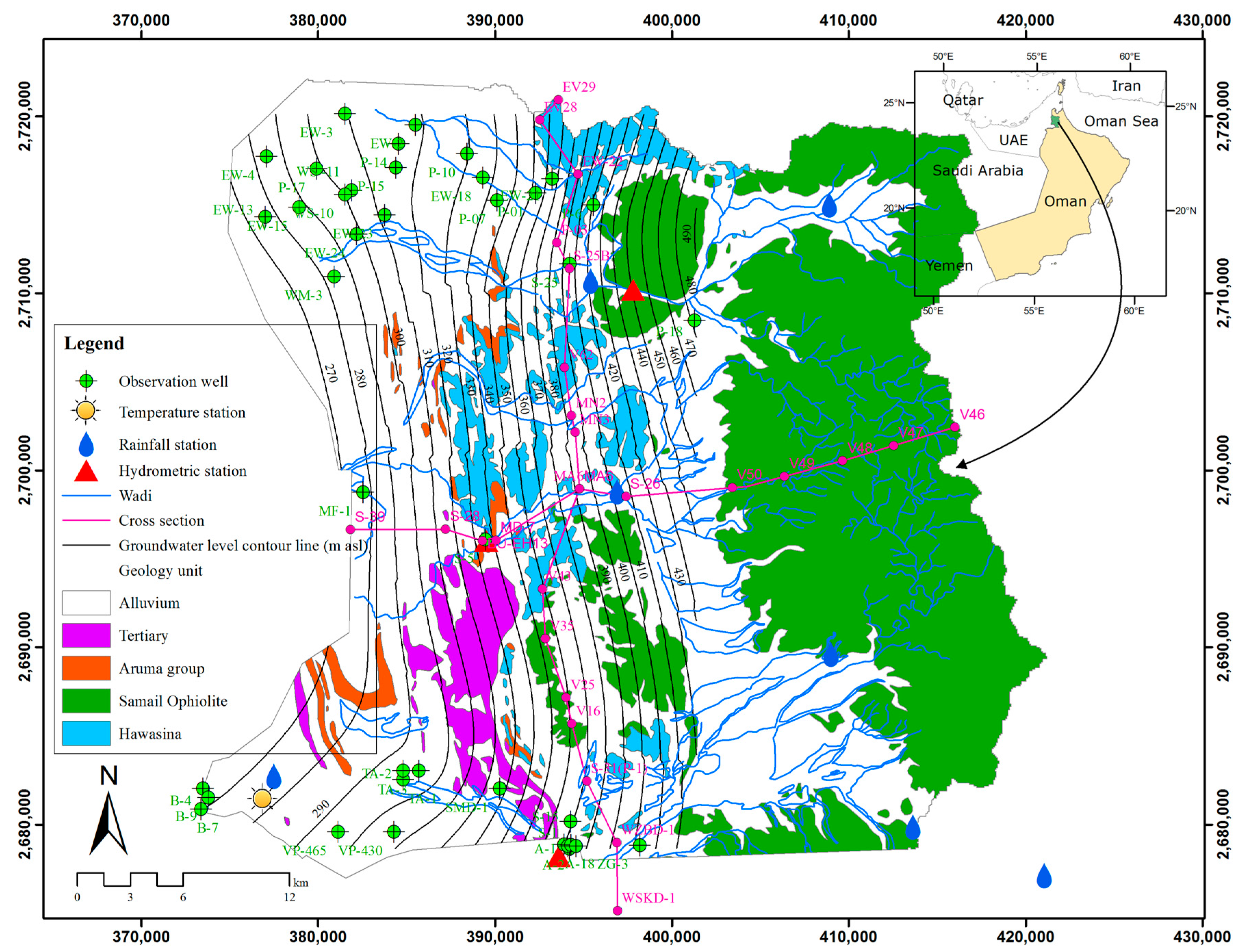
2.1. Study Area

The study area shown in Figure 1 is the Al-Buraimi region in the northwest portion of Oman, which is bounded to the east by the North Oman Mountains (NOMs) and to the west by the border with the UAE. It is approximately 1604 km2 in area and lies between 24°2′ N and 24°38′ N latitude and 55°44′ E and 56°14′ E longitude. The area has an arid climate with low humidity and long periods of little to no rainfall. Rainfall is highest in the mountains to the east and lowest in the plains to the west. Average annual rainfall ranges from 30 to 178 mm, with an average of 82 mm, which varies considerably from one year to another. Most of the rainfall is recorded from December to April, whereas the least and highest rainfall is observed in October and March, respectively. Maximum daytime temperature may reach 50 °C in the summer months. The long-term annual potential evapotranspiration is about 2700 mm. As a result of the arid to semi-arid climate, natural vegetation in the area tends to be fairly sparse, consisting predominantly of acacias and spiny bushes growing in the wadi (local name for the ephemeral) beds. However, winter rains are relatively common in the mountains area and maintain the water table within the alluvial sediments of the piedmont zone, which allows the cultivation of large palm-groves and market gardens around many of the villages [26,27,28].

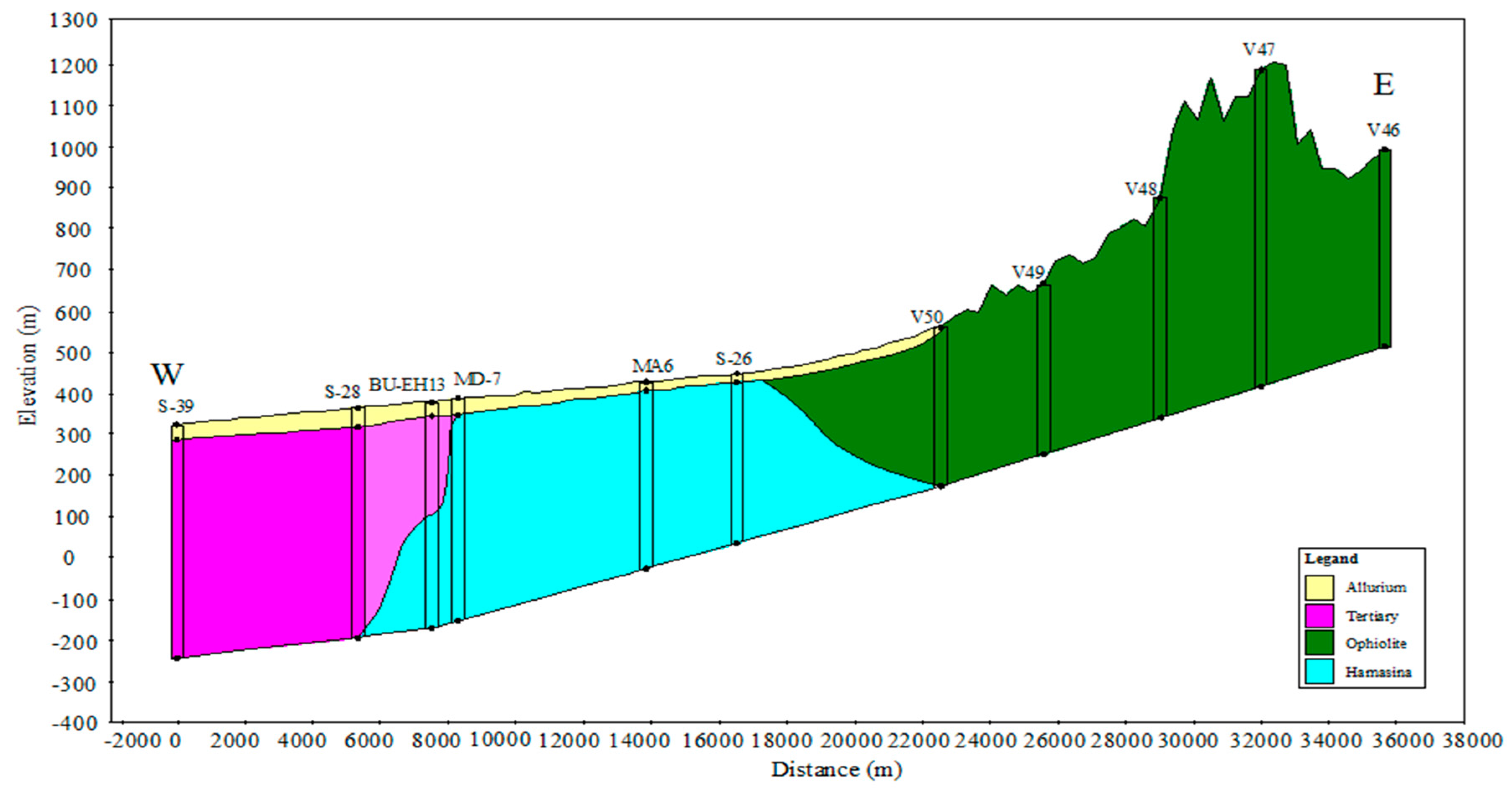
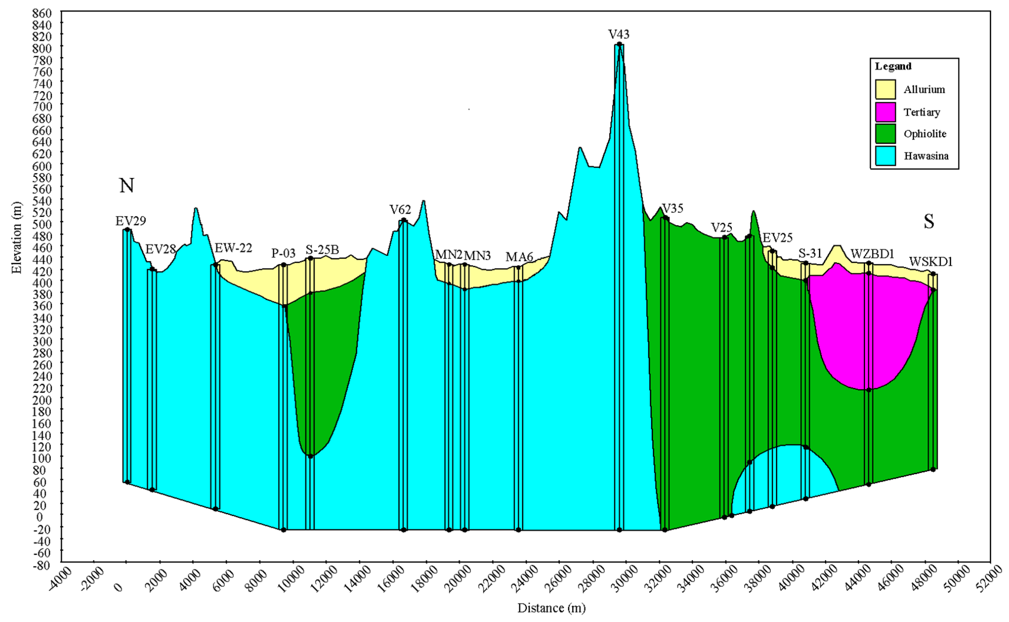
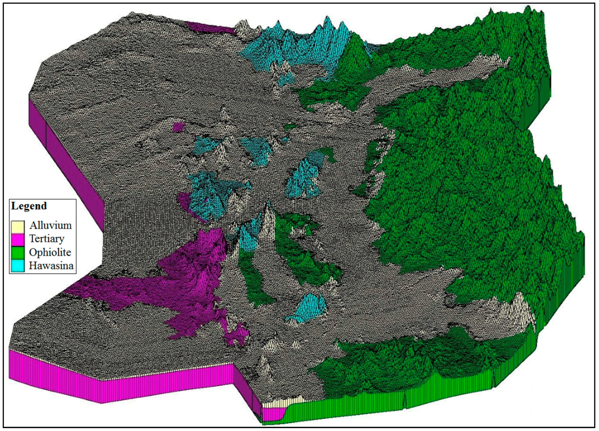
2.2. Geology and Hydrogeology

The geology of the study area is divided into three principal zones that include the Semail Nappes (Ophiolite), the Hawasina Nappes, and the post-nappe strata units (Aruma group, Tertiary and Quaternary Alluvium) (Figure 1). The Semail Nappes consist of crustal (outcrops) and mantle (NOMs) sequence ophiolite. The term “ophiolite” refers collectively to igneous rock that crops out in the study area with various dark colored, crystalline and microcrystalline characteristics. The Hawasina Nappe exposures mainly occur as broken hills in the eastern piedmont zone. They are elongated in a north–south direction and display extensive folding, faulting and thrusting features. The past-nappe strata consist of the Cretaceous Aruma Group and Tertiary bedrock that were deposited in a foredeep basin downfolded along the frontal margin of the nappes. Folding associated with mountain building in the Late Tertiary turned over the nappes and Tertiary strata into their present structural configurations. Afterwards, erosive processes associated with flowing water led to the deposition of alluvium (collectively to sand, gravel, silt, and clay) throughout the piedmont and alluvial fan zones to the west of the mountains. For more details about mountainous, piedmonts, and alluvial fan zones, refer to the Supplementary Materials.
In terms of regional hydrogeological significance, surface waters running off the mountainous portion of the study area recharge the piedmont and alluvial fan zones. Groundwater recharged into the fractures of the ophiolite during rainfall and runoff events gradually drains laterally and vertically downhill through the fractures towards the plains of the lower basin. Groundwater flow from the ophiolite is generally to the west. It is intercepted by aflaj (ancient water collection canals, known as aflaj (plural) or falaj (singular)) and a few wells at the mountain front and continues to the alluvial aquifers underlying the upper basin. When compared to other geological units, the hydrologic properties of the Hawasina Nappes are such that they are less important in terms of groundwater storage and transmission. Tertiary limestones may contain locally significant supplies of groundwater and also limited fractured characteristics. However, in the full extent of the water resources, the tertiary bedrock are not highly fractured in the study area, have low permeability, and yield little water. The alluvium in the piedmont and mountain front fan zones is the most important aquifer in the study area and is composed of an unconsolidated mixture of ophiolite, chert, limestone and dolomite. The alluvium generally has good permeability and water yields, which vary only upon the coarseness of the alluvium, its degree of sorting and cementation, and overall saturation thickness [26,27,28,29,30,31,32,33].

2.3. Groundwater Conceptual Model

The conceptual model of the groundwater flow for the study area was developed using a proposed framework by Izady et al. [34]. As can be seen in Figure 1, groundwater flow in the study area generally occurs from the east (with levels close to 490 m a.s.l.) to the west (where levels may reach 270 m a.s.l.). An average groundwater level decline of 10.49 m has been observed over a 17-year research period, equivalent to 0.62 m per year due to over-exploitation of the aquifer and extensive outflow from west boundary toward UAE. Long term observations indicate that groundwater level fluctuations have been less significant in the upper (eastern) part of the study area during this period, owing to the receipt of considerable amounts of recharge originating in the hardrock and much less abstraction (e.g., P-18 in Figure 1). Water table oscillations and declines are more notable in the middle (central) part of the study area (e.g., S-25 in Figure 1), while steeper declines have been observed in the lower (western) part because of larger abstractions for domestic and agricultural purposes (e.g., EW-13 in Figure 1).
Although Ophiolite formation has a thickness of 8 to 15 km, Stanger [35] showed that circulation of the groundwater within the formation occurs principally at the depths in the range of 300 m or less and that no deeper sources of groundwater originating from beyond the depth of the ophiolite are indicated. Moreover, Dewandel et al. [36] pointed out that groundwater circulation in Oman ophiolite rocks takes place mostly in the fissured near-surface depths (e.g., upper 50 m), and to a lesser degree in the deeper tectonic fractures. A three-dimensional stratigraphic model representing the vertical and spatial extent of four principal hydro-geologic units (specifically, the Hawasina, ophiolite, Tertiary and alluvium) was generated using data collected from 119 drilled boreholes and 77 virtual boreholes (Figure 2, Figure 3 and Figure 4). Virtual boreholes were used as supporting points to increase the accuracy of the generated stratigraphy in places where the geologic unit is vertically uniform (e.g., point V47–V50 in Figure 3). The locations of these boreholes were determined by discussion with local experts and consultants in the study area. The total thickness of this model varies from 300 to 700 m in the different parts of the study area, with the alluvial portions ranging between 27 m and 77 m in thickness (for more details, refer to the Supplementary Materials).
The eastern boundary of the study area, in the highlands of the NOMs, is considered to represent a surface and groundwater divide. Because the northern and southern boundaries of the study area are approximately parallel with the general groundwater flow direction, that can be associated with no-flux groundwater conditions. The western boundary of the study area along the Oman–UAE border is considered as an outflow boundary toward the UAE.
Based on aquifer tests, values of hydraulic conductivity (K) at the basin scale for the alluvium aquifer vary from a minimum of 7.79 m/day (9.02 × 10⁻⁵ m/s) to a maximum of 116 m/day (1.34 × 10⁻³ m/s) while the regional specific yield ranges between 0.01 and 0.15. The regional hydraulic conductivity and specific yield of the ophiolite were estimated as 1.0 × 10⁻⁶ m/s and 0.018, respectively. The hydrodynamic properties of Tertiary formations are higher than the ophiolite in the study area and estimated as 1.0 × 10⁻⁵ m/s and 0.02 for hydraulic conductivity and specific yield, respectively [26,27,28,29,30,31,32,33].
Annual artificial groundwater abstraction (withdrawal) from agricultural (24.2 Mm3; 90%) and domestic (2.4 Mm3; 10%) wells is approximately 26.6 Mm3 and from aflaj is 2.2 Mm3 [21]. Izady et al. [37] applied optimization-based water-table fluctuation (WTF) method combined with a groundwater balance model to estimate groundwater recharge for the study area. Long-term annual direct groundwater recharge from rainfall and return flow from irrigation over the model domain were estimated as 24.62 and 5.71 Mm3, respectively. The values estimated by Izady et al. [37] were used as an initial value for the groundwater flow modeling.

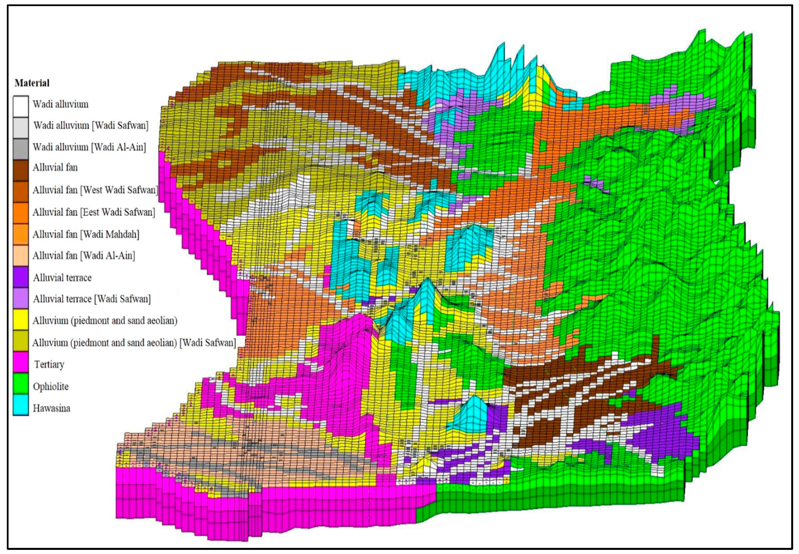
2.4. Model Setup and Structure

Fully transient simulation was conducted for the 1996–2013 period for the groundwater flow modeling in the Al-Buraimi region. Model calibration and validation were carried out for the period of October 1996 to September 2008 and October 2008 to September 2013, respectively. The generated stratigraphic model was used to define layer elevations and materials for the numerical model. In fact, elevations for four layers grid cells were taken from the generated stratigraphic model in which the lithology and elevations were inherited from the stratigraphic model that encompasses the cell (Figure 5). This process led to accurate grids so that the developed conceptual model in the previous section was mapped to simulate the groundwater flow.
Stress period, time step, and time unit was implemented as monthly, monthly, and daily, respectively. A regular mesh and a block centered finite difference grid with 0.125 km2 cells (250 m × 500 m) with a total of 184 rows, 108 columns and 4 layers were considered. Vertically, it varies from 300 m to 700 m in different parts of the plain with the alluvial thickness in layer one ranging between 27 m and 77 m. As mentioned earlier, the west boundary of the study area is associated with a groundwater outflow path. For this boundary, specific head boundary condition was considered in which monthly measured groundwater level data from the existing observation wells on the model boundary were used to prescribe time-varying constant head boundaries. The hydraulic conductivity, specific yield and specific storage were assigned for different units in the model. The abstraction values corresponding to all agricultural and domestic wells were assigned. The recharge rates computed by the optimized combined WTF and groundwater balance methods [37] were accounted for as an initial value in the model. The groundwater contour lines as an initial head, obtained from the observation wells, were generated using Empirical Bayesian Kriging (EBK) interpolation method for the October 1996. It is worth noting that the results of four different Inverse Distance Weighting (IDW), Spline, Ordinary Kriging (OK) and EBK interpolation methods were compared for the study area in which the performance of EBK interpolation method was better than other methods [38].
Model calibration was accomplished by varying values for a set of parameters that aims at matching simulated groundwater levels with the field observations. The set of parameters included hydraulic conductivity, specific yield, and specific storage values. The model was initially calibrated by trial and error to understand the response of the model to parameter changes. Afterward, the PEST algorithm [39] was used to achieve optimum calibrations using 24 observation wells as control points. Three different performance criteria were used to evaluate the effectiveness of the model and its ability to make predictions for the calibration and validation periods. These consisted of coefficient of determination (R2), Root Mean Square Error (RMSE) and Normalized Root Mean Square Error (NRMSE) approaches. A weighted average method is used for the overall performance of the method. The NRMSE approach was employed because the range of groundwater level fluctuation in the calibration and validation periods was different for each observation well [40]. The NRMSE for whole plain was calculated as follows:
Weighted RMSE = i = 1 N RMSE i × a i A
Weighted drawdown = i = 1 N Δ h i × a i A
Normalized RMSE = Weighted RMSE Weighted drawdown
where i refers to the observation well, N is number of observation wells, a is the area of Thiessen polygon i, A is the total model area, and ∆h is the difference between maximum and minimum groundwater level fluctuation for each observation well.

2.5. Standardized Precipitation Index

The Standardized Precipitation Index (SPI) was designed by McKee et al. [25] to quantify the precipitation deficit for multiple time scales. Computation of the SPI requires fitting a probability distribution to aggregated monthly precipitation series (e.g., 3, 6, 12, 24 months, etc.), computing the non-exceedence probability related to such aggregated values and defining the corresponding standard normal quantile as the SPI. McKee et al. [25] assumed an aggregated precipitation gamma distributed and used a maximum likelihood method to estimate the parameters of the distribution. In this study, the SPI was calculated on 12-month time scale, which corresponds to the past 12 months of observed precipitation.

3. Results and Discussion

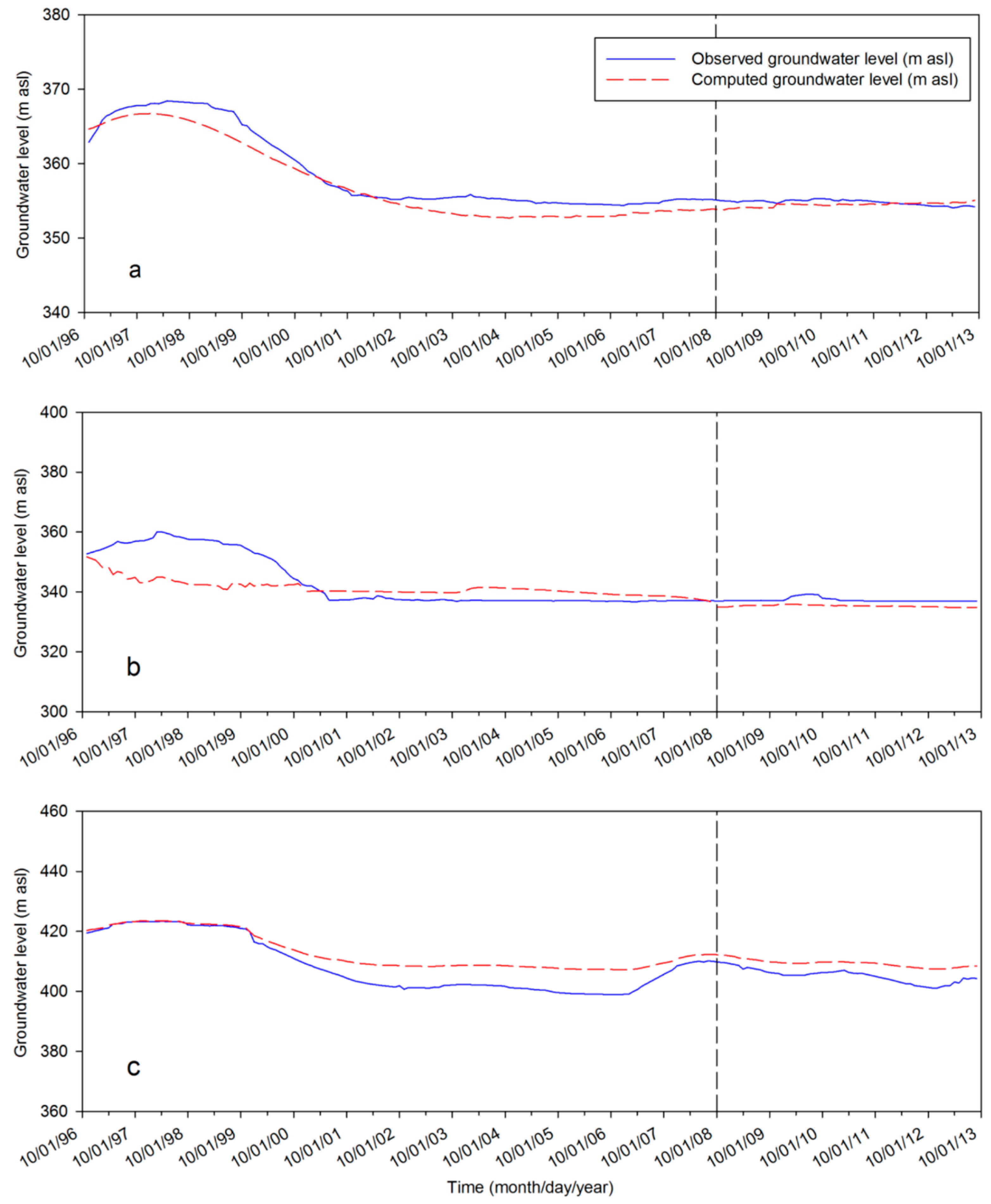
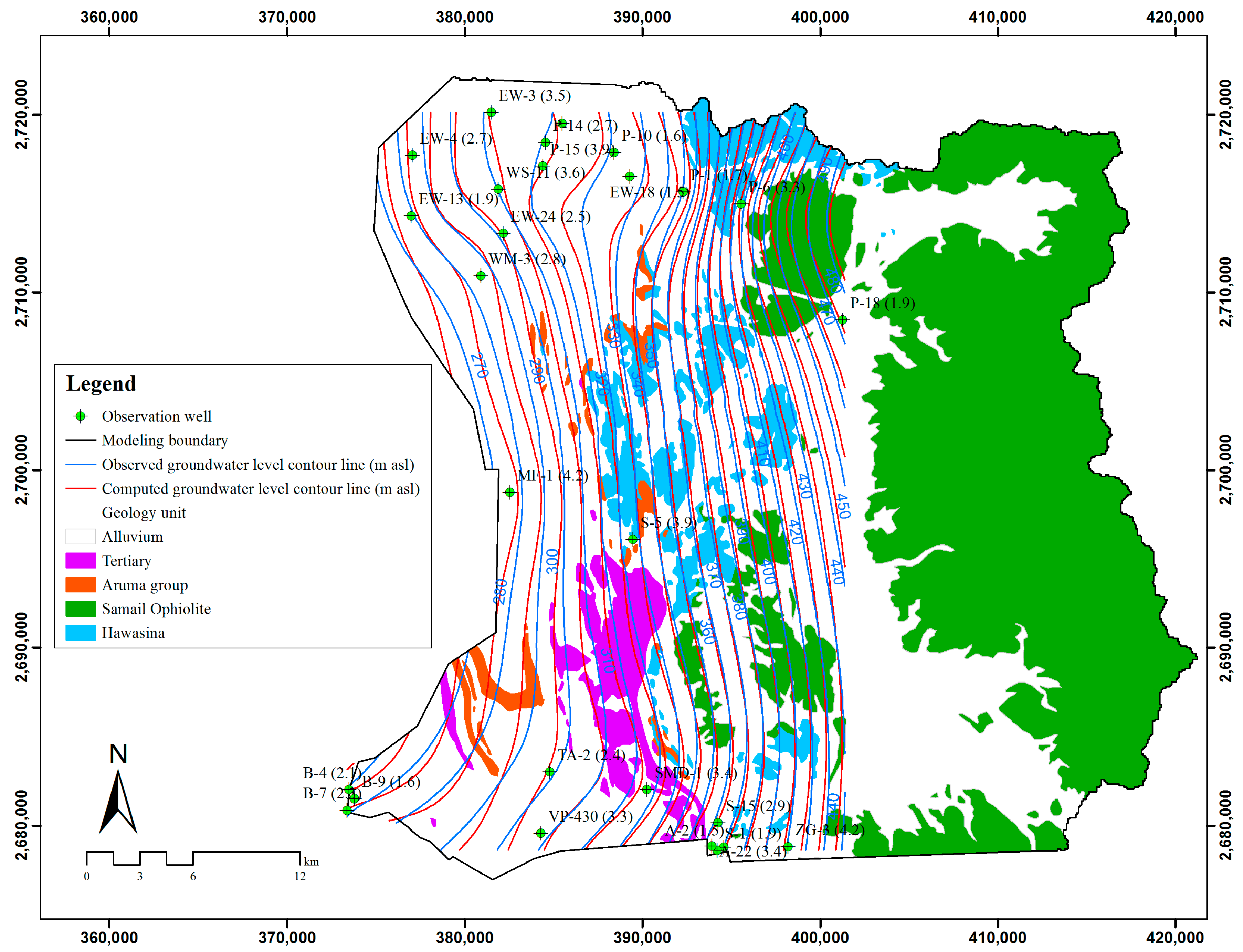
3.1. Model Calibration

The model calibration was carried out for the period October 1996 to September 2008. During the calibration, some of the initial parameter values were modified by trial and error in order to adjust the conceptual model. To cope with the numerous parameters and large study area, the PEST algorithm [39] was employed for auto-calibration. The calibrated parameters were hydraulic conductivity, specific yield and specific storage of the aquifer.
Table 1 and Figure 5 show calibrated hydrodynamic properties of the study area for the different geological units. The alluvium was sub-zoned into four different recent wadi alluvium, alluvial fan, alluvial terrace, and piedmont and sand dune units during the calibration process. Moreover, specific geological units were considered for wadi Safwan because of clustering most of the observation wells and serving as the primary aquifer of the study area. The recent wadi alluvium unit has the highest hydraulic conductivity (107 to 126 m/day) while the piedmont and sand dune unit has the lowest (7.3 to 11.2 m/day) over the study area. The hydraulic conductivity of the alluvial fan unit, as the second highest value, ranges from 22.7 to 44.80 m/day in which the west wadi Safwan has the lowest hydraulic conductivity. In addition, the horizontal hydraulic conductivity of Tertiary, ophiolite and Hawasina geologic units are estimated as 3.60 × 10⁻⁵, 1.12 × 10⁻⁵, and 1.04 × 10⁻⁸ m/s, respectively. The specific yield of the alluvium geologic unit varies between 0.035 and 0.15 in which wadi safwan and alluvial terrace units have respectively greatest and smallest values. In fact, specific yield of the different alluvium geological units exhibit the same trend as hydraulic conductivity over the study area. Moreover, the Tertiary, ophiolite and Hawasina geologic units collectively have a specific yield of 0.001. The specific storage of the alluvium geologic unit varies between 4.06 × 10⁻⁵ and 1.74 × 10⁻⁵ for the wadi alluvium and alluvial fan geological units. Furthermore, the specific storage of the Tertiary, ophiolite and Hawasina geologic units are estimated as 3.74 × 10⁻⁴, 4.50 × 10⁻⁴, and 1.00 × 10⁻⁵ m−1, respectively. After determining the optimum values for hydrodynamic properties, groundwater recharge values, obtained from Izady et al. [30], were modified by trial and error to obtain the smallest error for all control points. Results show that recharge occurs mainly through the wadi channel bed and therefore, the recharge at the recent wadi alluvium is high in comparison to other areas within the region. The regional-scale recharge varies from 11.76 to 43.94 million cubic meters (MCM), with an average of 18.09 MCM over the study area.
The model performance statistics for the calibration period are given in the Table 2. The Al-Buraimi study area is characterized by the remarkable geological and hydrogeological diversity and is constituted of unevenly scattered hardrock terrains and very thin alluvium in comparison with hardrock thickness (Figure 3 and Figure 4). Therefore, for the study area, with a total difference in groundwater level in the order of 228 m and 12-year monthly calibration period, a RMSE of 2.71 m is considered quite reasonable. The RMSE was normalized with regard to the groundwater level fluctuations of each observation well. For the whole study area, a normalized RMSE of 18% is a satisfactory result.
Contour lines based on the observed and computed groundwater levels are plotted for the last time step (September 2008) of the calibration period in Figure 6. It is seen that the patterns of observed and computed groundwater levels were similar. In such a regional-scale (1604 km2), high degree of aquifer heterogeneity/anisotropy and hydrological complexity (fractured hardrock and porous medium), the resulted match between computed and observed groundwater levels is a good indication of model accuracy. The RMSE performance criteria for the calibration period are also shown in Figure 6. The spatial distribution of the RMSE is fairly uniform, which are scattered throughout the entire plain.
The comparison between observed and computed groundwater levels are shown in Figure 7 for the observation wells P-1, S-5 and ZG-3 (results for all observation wells are available in the Supplementary Materials). These observation wells are located at the piedmont alluvium zone between mountainous and alluvial fan zones. The piedmont alluvium zone at the mountain front is hydrologically important in that it acts as a transition zone for both surface and groundwater that provides the alluvium downstream with groundwater recharge and storage. Surface water from the mountainous zone is flowing over a wide area by numerous wadis (ephemerals) on the coalescing alluvial fans of the piedmont zone. The gravely alluvium enhances infiltration to the shallow alluvium aquifer in the plain area. Therefore, observation wells P-1, S-5 and ZG-3 are selected because of their unique locations in the piedmont and transition zone to monitor the subsurface movement of water from mountainous to the alluvial fan zone. Figure 7 shows that the simulation mimics the trend of groundwater levels and captures the groundwater system behavior for the 12-year monthly calibration period in the complicated hardrock–alluvium geologic setting.
The validation results of observation wells are shown in Table 2 and Figure 7. The model performance is similarly good as the calibration results, indicating remarkable predictive ability of the calibrated model. The observed and computed groundwater contour lines of the last stress period of the validation (September 2013) along with their RMSE of each observation well are shown in Figure 8. This normalized RMSE is 32% for the validation period, which is acceptable regarding the complex hardrock–alluvium geological setting of the study area, the number of observation wells, the model resolution, the accuracy of water-table data, and the scale of the study area.

3.2. Groundwater Balance and Sustainable Groundwater Extraction

The annual groundwater budget components were calculated from October 1996 to September 2013 in a “water year” scale (period between 1 October of one year and 30 September of the next one). The groundwater budget components of the study area are given in Table 3. The long term regional groundwater recharge from rainfall and return flow provides 18.09 Mm3/year. Note that remarkable groundwater recharge produced by relatively high-intensity rainfall occurred in 1996–1997 and 2006–2007 water-years. The long term groundwater outflow from the study area toward UAE side is equivalent to 32.79 Mm3/year. The artificial groundwater abstraction from different sources is estimated as 27.3 Mm3/year. The groundwater balance components show a mean annual deficit of 41.99 Mm3.
The source of long-term reliable recharge to the alluvial aquifer in the study area is the drainage from the fractured eastern mantle sequence ophiolite toward the alluvial zone. Therefore, the subsurface groundwater flux from eastern ophiolite mountains is separately estimated (Table 4). The results show that the long-term lateral groundwater flux ranges from 4.23 to 11.69 Mm3/year, with an average of 5.67 Mm3/year drains from the fractured eastern ophiolite mountains into the alluvial zone. Along with natural recharge to the alluvial aquifer, this subsurface groundwater flux is sufficient to support the groundwater flow to the downstream alluvial basin between two substantial recharge events.
Sustainable groundwater extraction rate was also estimated for the long-term and different wet, normal and dry periods based on standardized precipitation index (SPI). Table 3 shows climate condition along with SPI values for the study area in which 1996–1997 and 2006–2007 water-years are considered as wet periods due to high rainfall amount of the mentioned years. In addition, five consecutive years from October 1999 to September 2004 as well as 2008–2009 year are treated as dry periods. The long-term regional groundwater sustainable groundwater extraction is 18.09 Mm3/year for 17-years. It is also, respectively, estimated as 14.51, 16.31, and 36.00 Mm3/year for dry, normal, and wet periods based on SPI climate condition. It is found that even with the exclusion of abstractions, the water budget of the aquifer is still deficit due to the high outflows toward UAE side, even for normal years. Indeed, groundwater discharge towards the UAE side is an important component in the water budget and actually exceeds the amount of groundwater extraction. Even if the groundwater pumping rate is restricted within the sustainable groundwater extraction, large water budget deficit will remain because natural recharge is not sufficient to sustain lateral groundwater outflow to the UAE side. It is known that heavily abstraction is taking place at the western side of the study area inside UAE (Davison 1982); the volume of such abstraction is not precisely known and was not considered in the current developed groundwater model. Therefore, steeper declines have been observed in the western part of the study area in comparison with central and eastern parts. As a result, the groundwater outflow toward UAE side is mostly affected by the abstraction in the UAE side and therefore the water budget shows a negative balance even with the exclusion of Oman side abstractions.
It is worth noting that the west boundary at the UAE side is highly affected by the groundwater outflow which is attributed to the groundwater overexploitation in the UAE side. This boundary is defined as the Dirichlet condition with prescribed time-variable head values in which the boundary head values are estimated by the interpolation of measured heads at the observation wells along the boundary [38]. The interpolation as well as the measured heads will introduce uncertainty to the boundary values of the model, which in turn will propagate to the simulated flux out of the boundary. Therefore, the incomplete knowledge of these boundary head values will cause considerable uncertainty of outflow across the boundary estimated from the model. Moreover, the abstraction at the western side of the study area inside the UAE was not considered in the current developed model due to the lack of information. Hence, incorporating abstraction and groundwater level data from the UAE side in the model may help to reduce the uncertainty of the outflow.

4. Concluding Remarks

A numerical model was developed to simulate groundwater flow and to estimate sustainable groundwater extraction in the Al-Buraimi region, located at the Oman–UAE border. This study provides a significant contribution to the understanding of the groundwater resources in the region. The developed model integrates the prepared stratigraphic model with hydrogeological information available for the region in order to estimate sustainable groundwater extraction for different dry, normal, and wet climate periods based on SPI index. In addition, subsurface flux from the fractured eastern mantle sequence ophiolite into the downstream alluvial aquifer is assessed. The results show that the long-term regional groundwater sustainable groundwater extraction is 18.09 Mm3/year for 17 years, while is, respectively, estimated as 14.51, 16.31, and 36.00 Mm3/year for dry, normal, and wet periods based on SPI climate condition. Moreover, long-term lateral groundwater flux ranging from 4.23 to 11.69 Mm3/year, with an average of 5.67 Mm3/year drains from the fractured eastern ophiolite mountains toward the alluvial zone. These results come as a substantial finding of this study particularly when considering that no prior quantitative groundwater flow modeling had been conducted in this region.
The developed regional groundwater model and these findings would help decision makers to have a better understanding of the groundwater budget components in such important transboundary hardrock–alluvium aquifer, located at the Oman–UAE border. It would assist decision makers to improve existing strategies to enhance the decision making for future developments in different climate condition. As indicated by the imbalance of the water budget analyzed during this study, the groundwater system is under transient state shown by high outflow which indicates notable abstraction rates across the border. This study, however, was carried out inside Oman and no data from the UAE side was available. The lack of data is not only limited to abstraction rates but also to aquifer system understanding, hydrodynamic properties, observation wells data among others. It would have been optimum to develop the model in both regions, which requires mutual understanding and interest. The developments of better understanding of the technical issues that are facing the shared resources are fundamental to ensure groundwater sustainability and hence secure agricultural, domestic and industrial activities. This study provides the water balance estimation across the boundary, which gives important boundary data for further modeling efforts in UAE side. Once technical aspects are agreed upon, parties can agree on policy and governance of the resources. In fact, regional cooperation is required to address policy, ownership and technical aspects to achieve sustainability of groundwater resources for this shared aquifer.

Supplementary Materials

The following are available online at www.mdpi.com/2073-4441/9/3/161/s1. The online version of this article contains Supplementary Materials.

Acknowledgments

Authors would like to thank the Sultan Qaboos University (SQU) for the financial support under grant # CL/SQU-UAEU/14/04. Thanks are due to the Ministry of Regional Municipalities and Water Resources (MRMWR) for providing the data.

Author Contributions

All authors contributed equally to this research.

Conflicts of Interest

The authors declare no conflict of interest.

References

  1. Wolf, A.T.; Yoffe, S.B.; Giordano, M. International waters: Identifying basins at risk. Water Policy 2003, 5, 29–60. [Google Scholar]
  2. Hayton, R.; Utton, A.E. Transboundary groundwaters: The Bellagio draft treaty. Nat. Resour. J. 1989, 29, 663–722. [Google Scholar]
  3. Bourne, C. The International Law Commission’s draft articles on the law of international watercourses: Principles and planned measure. Colo. J. Int. Environ. Law Policy 1992, 3, 65–92. [Google Scholar]
  4. Campana, M.E. Foreword: Transboundary ground water. Groundwater 2005, 43, 646–652. [Google Scholar] [CrossRef]
  5. Fendek, M.; Fendekova, M. Transboundary flow modeling: The Zohor depression of Austria and the Slovak Republic. Groundwater 2005, 43, 717–721. [Google Scholar] [CrossRef] [PubMed]
  6. Bittinger, M.W. Survey of interstate and international aquifer problems. Groundwater 1972, 10, 44–54. [Google Scholar] [CrossRef]
  7. Froukh, L.J. Transboundary groundwater resources of the West Bank. Water Resour. Manag. 2003, 17, 175–182. [Google Scholar] [CrossRef]
  8. Rainwater, K.; Stovall, J.; Frailey, S.; Urban, L. Transboundary impacts on regional ground water modeling in Texas. Groundwater 2005, 43, 706–716. [Google Scholar] [CrossRef] [PubMed]
  9. Chermak, J.M.; Patrick, R.H.; Brookshire, D.S. Economics of transboundary aquifer management. Groundwater 2005, 43, 731–736. [Google Scholar] [CrossRef] [PubMed]
  10. Weinthal, E.; Vengosh, A.; Marei, A.; Gutierrez, A.; Kloppmann, W. The water crisis in the Gaza strip: Prospects for resolution. Groundwater 2005, 43, 653–660. [Google Scholar] [CrossRef] [PubMed]
  11. Cardona, A.; Nigro, N.; Sonzogni, V.; Storti, M. Finite difference model for evaluating the recharge of the Guarani aquifer system on the Uruguayan-Brazilian border. Mec. Comput. 2006, 25, 1479–1496. [Google Scholar]
  12. Siegfried, T.; Kinzelbach, W. A multi-objective discrete stochastic optimization approach to shared aquifer management: Methodology and application. Water Resour. Res. 2006, 42, 1–15. [Google Scholar] [CrossRef]
  13. Katic, P.G. Spatial dynamics and hydro-economic modeling of transboundary aquifers. In Proceedings of the ISARM2010 International Conference “Transboundary Aquifers: Challenges and New Directions”, UNESCO, Paris, France, 6–8 December 2010.
  14. Gossel, W.; Sefelnasr, A.; Wycisk, P. Modelling of paleo-saltwater intrusion in the northern part of the Nubian Aquifer System, Northeast Africa. Hydrogeol. J. 2010, 18, 1447–1463. [Google Scholar] [CrossRef]
  15. Ganoulis, J.; Skoulikaris, C. A Conceptual Model for Implementing Integrated Transboundary Water Resources Management (ITWRM). In Proceedings of the Building Knowledge Bridges for a Sustainable Water Future, Gamboa, Panama, 21–24 November 2011; p. 99.
  16. Milman, A.; Ray, I. Interpreting the unknown: Uncertainty and the management of transboundary groundwater. Water Int. 2011, 36, 631–645. [Google Scholar] [CrossRef]
  17. Öztan, M.; Axelrod, M. Sustainable transboundary groundwater management under shifting political scenarios: The Ceylanpinar Aquifer and Turkey–Syria relations. Water Int. 2011, 36, 671–685. [Google Scholar] [CrossRef]
  18. Gillespie, J.; Nelson, S.T.; Mayo, A.L.; Tingey, D.G. Why conceptual groundwater flow models matter: A transboundary example from the arid Great Basin, western USA. Hydrogeol. J. 2012, 20, 1133–1147. [Google Scholar] [CrossRef]
  19. Szucs, P.; Virag, M.; Zakanyi, B.; Kompar, L.; Szanto, J. Investigation and water management aspects of a Hungarian-Ukrainian transboundary aquifer. Water Resour. 2013, 40, 462–468. [Google Scholar] [CrossRef]
  20. Voss, K.A.; Famiglietti, J.S.; Lo, M.; Linage, C.; Rodell, M.; Swenson, S.C. Groundwater depletion in the Middle East from GRACE with implications for transboundary water management in the Tigris-Euphrates-Western Iran region. Water Resour. Res. 2013, 49, 904–914. [Google Scholar] [CrossRef] [PubMed]
  21. Voss, C.I.; Soliman, S.M. The transboundary non-renewable Nubian Aquifer System of Chad, Egypt, Libya and Sudan: Classical groundwater questions and parsimonious hydrogeologic analysis and modeling. Hydrogeol. J. 2014, 22, 441–468. [Google Scholar] [CrossRef]
  22. Al-Rawabdeh, A.; Al-Ansari, N.; Al-Taani, A.; Al-Khateeb, F.; Knutsson, S. Modeling the risk of groundwater contamination using modified DRASTIC and GIS in Amman-Zerqa Basin, Jordan. Open Eng. 2014, 4, 264–280. [Google Scholar] [CrossRef]
  23. Sefelnasr, A.; Gossel, W.; Wycisk, P. Groundwater management options in an arid environment: The Nubian Sandstone Aquifer System, Eastern Sahara. J. Arid Environ. 2015, 122, 46–58. [Google Scholar] [CrossRef]
  24. Alley, W.M.; Leake, S.A. The journey from safe yield to sustainability. Ground Water 2004, 42, 12–16. [Google Scholar] [CrossRef] [PubMed]
  25. McKee, T.B.; Doesken, N.J.; Kleist, J. The relationship of drought frequency and duration to time scales. In Proceedings of the 8th Conference on Applied Climatology, Anaheim, CA, USA, 17–22 January 1993; American Meteorological Society: Boston, MA, USA, 1993; Volume 17, pp. 179–183. [Google Scholar]
  26. Turner, W.R.; Forbes, A.S.; Rapp, J.R. Groundwater Resources of the Wadi Safwan Area; Report: PAWR I-86-9; Public Authority for Water Resources (PAWR): Muscat, Oman, 1986.
  27. Kaczmarek, M.B.; Brook, M.; Haig, T.; Read, R.E.; George, D. Water Resources Assessment and Hydrogeology of the Mahdah Watershed, Northern Oman; Ministry of Water Resources: Muscat, Oman, 1993.
  28. MRMWR: Ministry of Regional Municipalities and Water Resources. Consultancy for Drilling and Aquifer Testing Program of Buraimi at Ad Dhairah Region; Ministry of Regional Municipalities, Environment and Water Resources: Muscat, Oman, 2004.
  29. Davison, W.D. Results of Test Drilling in the Buraimi Area, Sultanate of Oman; Water Supply Paper 1; Public Authority for Water Resources (PAWR): Muscat, Oman, 1982.
  30. Kaczmarek, M.B. Hydrogeology and Groundwater Availability Buraimi Production Well-Field, Part I—Final Report; Director General Water, Water Projects, Hydrogeology Section; Ministry of Water Resources: Muscat, Oman, 1988.
  31. Kaczmarek, M.B.; Brook, M.; Haig, T.; Read, R.E.; George, D. Water Resources Assessment and Hydrogeology of Wadi Safwan and Wadi Sharm, Northern Oman; Ministry of Water Resources: Muscat, Oman, 1993.
  32. Kaczmarek, M.B.; Brook, M.; Haig, T.; Read, R.E.; George, D. Water Resources Assessment and Hydrogeology of the Zarub Gap Watershed, Wadi Musayliq and Wadi Al Ayn, Northern Oman; Ministry of Water Resources: Muscat, Oman, 1993.
  33. Onanda, M.; Price, V.; Jolley, T.; Stuck, A.; Hall, R. Water Balance Computation for the Sultanate of Oman; Final Report; Ministry of Regional Municipalities and Water Resources: Muscat, Oman, 2013.
  34. Izady, A.; Davary, K.; Alizadeh, A.; Ziaei, A.N.; Alipoor, A.; Joodavi, A.; Brusseau, M.L. A framework toward developing a groundwater conceptual model. Arab. J. Geosci. 2014, 7, 3611–3631. [Google Scholar] [CrossRef]
  35. Stanger, G. The Hydrogeology of the Oman Mountains. Ph.D. Thesis, Department of Earth Sciences, The Open University, Milton Keynes, UK, 1986; p. 355. [Google Scholar]
  36. Dewandel, B.; Lachassagne, P.; Boudier, F.; Al-Hattali, S.; Ladouche, B.; Pinault, J.L.; Al-Suleimani, Z. A conceptual hydrogeological model of ophiolite hard-rock aquifers in Oman based on a multi-scale and a multidisciplinary approach. Hydrogeol. J. 2005, 13, 708–726. [Google Scholar] [CrossRef]
  37. Izady, A.; Abdalla, O.; Joodavi, A.; Karimi, A.; Chen, M.; Tompson, A.F.B. An efficient methodology for groundwater recharge estimation in arid hardrock-alluvium aquifers using combined water-table fluctuation and groundwater balance methods. Hydrol. Process. 2017. submitted for publication. [Google Scholar]
  38. Izady, A.; Abdalla, O.; Ahmadi, T.; Chen, M. An efficient methodology to design optimal groundwater level monitoring network in Al-Buraimi region, Oman. Arab. J. Geosci. 2017, 10, 26. [Google Scholar] [CrossRef]
  39. Doherty, J. PEST: Model Independent Parameter Estimation, User’s Manual; Watermark Computing: Brisbane, Australia, 1998. [Google Scholar]
  40. Izady, A.; Davary, K.; Alizadeh, A.; Ziaei, A.N.; Akhavan, S.; Alipoor, A.; Joodavi, A.; Brusseau, M.L. Groundwater conceptualization and modeling using distributed SWAT-based recharge for the semi-arid agricultural Neishaboor plain, Iran. Hydrogeol. J. 2015, 23, 47–68. [Google Scholar] [CrossRef]
  41. Tsakiris, G.; Vangelis, H. Towards a drought watch system based on spatial SPI. Water Resour. Manag. 2004, 18, 1–12. [Google Scholar] [CrossRef]
Figure 1. Location of the study area in the Al-Buraimi region, Oman–UAE border along with geological map, meteorological stations, wadi network, hydrometric stations and observation wells. Groundwater level contour lines in the study area showing the groundwater flow direction from east to west.
Water 09 00161 g001
Figure 2. 3D view of the developed stratigraphy for the Al-Buraimi region.
Water 09 00161 g002
Figure 3. The V46-S39, east–west cross-section (m a.s.l. is meters above sea level) (see Figure 1 for the location).
Water 09 00161 g003
Figure 4. The EW29-WSKD1, north–south cross-section (m a.s.l. is meters above sea level) (see Figure 1 for the location).
Water 09 00161 g004
Figure 5. 3D view of the finite difference grid with four layers and different materials for the Al-Buraimi region.
Water 09 00161 g005
Figure 6. Observed (blue line) and computed (red line) groundwater level contour lines for the AL-Buraimi region (October 2008) (m a.s.l. is meter above sea level). The starting date of the calibration period is October 1996. The numbers in the parenthesis aside observation well’s name are RMSE (unit in meter).
Water 09 00161 g006
Figure 7. Plots of observed and computed groundwater levels during the calibration (October 2000 to September 2010), and validation (October 2010 to September 2012) periods for: (a) P-1; (b) S-5; and (c) ZG-3 observation wells. The results for all observation wells are available in the Supplementary Materials.
Water 09 00161 g007
Figure 8. Observed (blue line) and computed (red line) groundwater level contour lines for the AL-Buraimi study area (September 2013) (m a.s.l. is meter above sea level). The starting date of the validation period is October 2008. The numbers in the parenthesis aside observation well’s name are RMSE (unit in meter).
Water 09 00161 g008
Table 1. Calibrated hydrodynamic properties of the study area for the different geological units.
Geological UnitHydraulic Conductivity (m/Day)Specific YieldSpecific Storage (m−1)
HK *RangeSyRangeSs (m−1)Range
Wadi alluvium12663–1460.0820.01–0.152.90 × 10−51.0 × 10⁻⁵–4.0 × 10⁻⁴
Wadi alluvium (Wadi Safwan)10763–1460.1500.01–0.154.06 × 10−52.90 × 10⁻⁵–4.0 × 10⁻⁴
Wadi alluvium (Wadi Al-Ain)11663–1460.0930.01–0.152.90 × 10−52.90 × 10⁻⁵–4.0 × 10⁻⁴
Alluvial fan44.827–550.0450.01–0.151.74 × 10−52.90 × 10⁻⁵–4.0 × 10⁻⁴
Alluvial fan (West Wadi Safwan)22.727–550.1300.01–0.152.90 × 10−52.90 × 10⁻⁵–4.0 × 10⁻⁴
Alluvial fan (East Wadi Safwan)39.927–550.1300.01–0.152.90 × 10−52.90 × 10⁻⁵–4.0 × 10⁻⁴
Alluvial fan (Wadi Mahdah)35.027–550.0760.01–0.152.90 × 10−52.90 × 10⁻⁵–4.0 × 10⁻⁴
Alluvial fan (Wadi Al-Ain)44.127–550.1060.01–0.152.90 × 10−52.90 × 10⁻⁵–4.0 × 10⁻⁴
Alluvial terrace34.39–450.0340.01–0.151.74 × 10−52.90 × 10⁻⁵–4.0 × 10⁻⁴
Alluvial terrace (Wadi Safwan)14.79–450.1200.01–0.152.90 × 10−52.90 × 10⁻⁵–4.0 × 10⁻⁴
Alluvium (piedmont and sand dune)7.39–350.0350.01–0.153.11 × 10−52.90 × 10⁻⁵–4.0 × 10⁻⁴
Alluvium (piedmont and sand dune) (Wadi Safwan)11.29–350.1200.01–0.152.90 × 10−52.90 × 10⁻⁵–4.0 × 10⁻⁴
Tertiary3.11 (3.60 × 10⁻⁵) **1–40.0010.0006–0.00143.74 × 10−46.0 × 10⁻⁵–1.4 × 10⁻⁴
Ophiolite1.12 (1.30 × 10⁻⁵)0.08–20.0010.0006–0.00144.50 × 10−46.0 × 10⁻⁵–1.4 × 10⁻⁴
Hawasina0.0009 (1.0 × 10⁻⁸)8.60 × 10⁻⁷–8.60 × 10−50.0010.0006–0.00141.0 × 10−56.0 × 10⁻⁵–1.4 × 10⁻⁴
Notes: * HK is horizontal hydraulic conductivity, Sy and Ss are, respectively, specific yield and specific storage; ** Numbers in parentheses are horizontal hydraulic conductivity in meter per second (m/s).
Table 2. Model performance statistics for the calibration and validation periods.
PeriodWeighted RMSE (m)Weighted R2NRMSE (%)
Calibration2.710.6918
Validation3.470.6532
Table 3. The Annual groundwater balance components in million cubic meters along with climate condition for the October 1996 to September 2013.
PeriodSPI Values *Climate ConditionInflowOutflowBalance
QR **QAA **Qout **±ΔV
October 1996–September 19971.56Wet43.9435.0240.07−31.15
October 1997–September 19980.66Normal19.6232.9641.31−54.65
October 1998–September 1999−0.36Normal15.1331.3940.79−57.05
October 1999–September 2000−2.47Dry15.1931.5543.35−59.71
October 2000–September 2001−1.80Dry14.9130.1644.81−60.06
October 2001–September 2002−1.49Dry15.0927.1840.79−52.88
October 2002–September 2003−1.31Dry14.9825.9638.54−49.52
October 2003–September 2004−1.20Dry15.1526.5538.08−49.48
October 2004–September 20050.63Normal18.1726.8131.57−40.21
October 2005–September 20060.48Normal15.3825.9929.92−40.53
October 2006–September 20071.22Wet28.0726.0926.71−24.73
October 2007–September 20080.61Normal13.5725.0627.87−39.36
October 2008–September 2009−1.31Dry11.7625.3225.57−39.13
October 2009–September 20100.82Normal21.2023.8823.47−26.15
October 2010–September 2011−0.16Normal13.7224.0827.52−37.88
October 2011–September 20120.02Normal15.5623.1019.71−27.25
October 2012–September 20130.83Normal16.2023.0117.38−24.19
17-year average--18.0927.332.79−41.99
Notes: * The ranges of SPI values are 1.0–>2, −0.99–+0.99, and −1.0–<−2 for wet, normal, and dry climate condition, respectively [41]; ** QR is groundwater recharge from rainfall and return flow, QAA is artificial abstraction, Qout is the groundwater outflow toward UAE side, and ΔV is groundwater storage.
Table 4. The groundwater flux from the fractured eastern mantle sequence ophiolite toward the alluvium zone in million cubic meters.
PeriodQbf
October 1996–September 199711.69
October 1997–September 19987.79
October 1998–September 19996.31
October 1999–September 20006.04
October 2000–September 20015.80
October 2001–September 20025.51
October 2002–September 20035.30
October 2003–September 20045.14
October 2004–September 20055.11
October 2005–September 20066.09
October 2006–September 20074.87
October 2007–September 20084.64
October 2008–September 20094.50
October 2009–September 20104.68
October 2010–September 20114.34
October 2011–September 20124.40
October 2012–September 20134.23
17-year average5.67

