A Short-Term Water Demand Forecasting Model Using a Moving Window on Previously Observed Data

Abstract

In this article, a model for forecasting water demands over a 24-h time window using solely a pair of coefficients whose value is updated at every forecasting step is presented. The first coefficient expresses the ratio between the average water demand over the 24 h that follow the time the forecast is made and the average water demand over the 24 h that precede it. The second coefficient expresses the relationship between the average water demand in a generic hour falling within the 24-h forecasting period and the average water demand over that period. These coefficients are estimated using the information available in the weeks prior to the time of forecasting and, therefore, the model does not require any actual calibration process. The length of the time series necessary to implement the model is thus just a few weeks (3–4 weeks) and the model can be parameterized and used without there being any need to collect hourly water demand data for long periods. The application of the model to a real-life case and a comparison with results provided by another model already proposed in the scientific literature show it to be effective, robust, and easy to use.

1. Introduction

Water demands represent the driver of water distribution systems, and reliable demand forecasting represents a valid aid in simulating and managing such systems. Depending on the time horizon considered, water demand forecasts can be classified, as suggested by [1], into “strategic”, “tactical”, and “operational”.

Forecasts of a “strategic” type provide an estimate of water demands over long time horizons, spanning decades [2], and are intended to support long-term planning of water resource use or the design of water networks [3,4,5,6].

Forecasts of a “tactical” type provide an estimate of water demands over medium-term horizons of a few years [2] and are intended to support the management in interventions to upgrade and improve networks and installations [7,8].

Finally, forecasts of an “operational” type provide an estimate of water demands over short time horizons, ranging from one day to a few weeks [2], and are aimed at enabling optimal short-term (or real-time) management of the network devices and installations (pressure regulating valves, pumping stations, energy recovery systems, etc.) [9,10,11,12,13,14,15,16].

Focusing attention on the latter type of forecast, which the present study is specifically concerned with, a variety of models have recently been presented in the scientific literature (see, for example, [1,2,17] for a review of these models). The models differ in several respects—principally, in the time step considered, the type of input used, and the structure and approach on which the model is based.

The time step used typically ranges from a day [11,18] to an hour [12,19], or to as little as a quarter of an hour in the case of the model of [13]. There are also models with multiperiodicity, in which water demand is forecast at different time steps, for example on a daily and hourly basis, as in [10].

With regard to inputs, the majority of short-term forecasting models are based mainly on the historical series of demands observed in the previous week or month or year.

However, in some cases, climate factors such as precipitation, temperature, and humidity are also considered, as they can have a significant impact on water demand [19,20,21].

Finally, as far as approach is concerned, many of the models recently proposed in the literature are based on data-driven techniques such as artificial neural networks (ANNs) (e.g., [12,17,22,23,24,25], support vector machines (SVMs) (e.g., [26,27], fuzzy logic [28], projection pursuit regression (PPR), random forests (RMs) and multivariate adaptive regression splines (MARS) [12].

Other models, by contrast, are based primarily on the representation of the periodic patterns that typically characterize demand [13], possibly coupled with techniques of time series analysis, as in [10].

An important aspect that should be highlighted is the model’s parameterization, which is closely connected both to the approach and to the structure of the model itself.

The above-mentioned models are based on structures that can be more or less complex, but they are generally characterized by parameters whose values must be defined prior to the model’s application. For example, neural network models, by their very nature, require a calibration of weights and bias; a sufficiently long time series of historically observed data has to be used for this purpose in order for the network to be effectively trained, taking into account the variability in the water demand patterns that can be observed, for example, during the year. It is well known, in fact, that a neural network, when implemented in practice, is able to reliably reproduce/forecast data that fall within the range previously used for calibration, whereas it may produce poor results if applied to a set of data differing completely from those considered in the calibration phase [29,30]. Clearly, a neural network forecasting model calibrated on the basis of data relating to low demands—typical, for example, of a winter period—might perform poorly if then applied for forecasting in periods of high demand, such as in summertime. An analogous consideration applies for pattern-based models. For example, the model proposed by [10] requires at least one year of observations in order to define long-term periodic patterns, or seasonal fluctuations, as well as to characterize daily demand patterns, which vary from season to season. From an operational viewpoint, the need to have a time series of historically observed data for the network to which the forecasting model is to be applied can be a limiting factor to be taken into account when choosing the model’s structure.

In this paper, a short-term water demand forecasting model based on the use of a short series of data observed prior to the time, i.e., the hour, at which the forecast is made, is presented. The model is structured in such a way as to use, as input data, the hourly water demands observed over a few weeks prior to the time of the forecast and to deliver, as output, an hourly water demand forecast for the next 24 h. As illustrated in the sections that follow, some of the advantages of this model lie in the simplicity of the structure it is based on and the substantial absence of a calibration period. In fact, the parameters of this model simply change as time passes and are updated on the basis of the last, or most recent, observed data. Indeed, it is worth noting that this type of approach based on a moving window of previously observed data has been already used in other frameworks such as power demand forecasting [31], water meter under-registration [32], and meter tampering [33].

Below, the structure of the proposed forecasting model is presented (Section 2); the model is then applied to a real case study (Section 3), and the results obtained are analyzed and compared with those provided by another short-term forecasting model already proposed in the scientific literature (Section 4). Finally, in Section 5, some concluding considerations are presented.

2. The Proposed Model

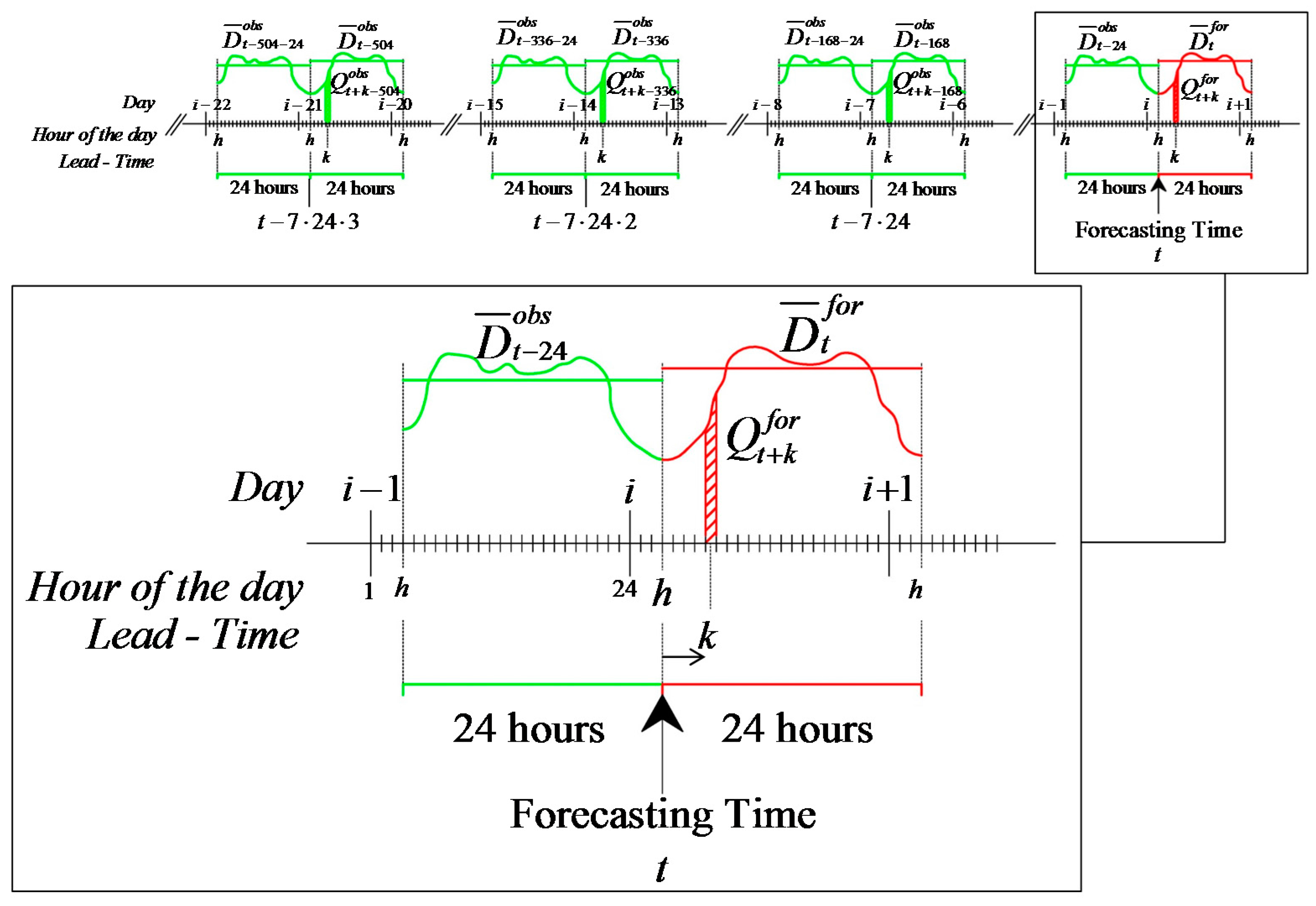
With reference to the diagram in Figure 1, let us assume an hourly time step and let i (with i = 1, 2,…, 365) be a generic day of the year and h (with h = 1, 2,…, 24) be a generic hour of the day. Let the time t denote a generic hour of the year (counted from the beginning of the year) in which the forecast is made. Assuming that the forecast is made at the h-th hour of the i-th day of the year, the time t will be equal to:

$$t=24(i-1)+h$$

(1)

Finally, let k (with $k=1,2,...,K=24$) be the forecast lead time.

The model comprises two steps. In the first step, the average water demand over 24 h which represents the forecasting time window is estimated. In the second step, relying on this forecast, the average hourly water demand in each hour included in the window is estimated.

More precisely, the average water demand ${\overline{D}}_t^{for}$ for the K = 24 h following the time t is estimated by means of the following relation:

$${\overline{D}}_t^{for}={\mathsf{\alpha }}_t{\overline{D}}_{t-24}^{obs}$$

(2)

where ${\overline{D}}_{t-24}^{obs}$ is the observed average water demand in the 24 h prior to the forecasting time t (or from t − 24 to t) and ${\mathsf{\alpha }}_t$ is a coefficient having a specific value for the 24-h horizon that starts at the time t. In particular, it represents the expected ratio between the average water demand over the 24 h included in the forecasting interval and the average water demand over the 24 h that precede that interval.

Once the average water demand ${\overline{D}}_t^{for}$ is known, we can go on to estimate the average hourly water demand $Q_{t+k}^{for}$ for the time t + k (with k = 1, 2,…, K = 24) by means of the following relation:

$$Q_{t+k}^{for}={\mathsf{\beta }}_{t,k}{\overline{D}}_t^{for}$$

(3)

where the coefficient ${\mathsf{\beta }}_{t,k}$ refers to the specific lead time k of the time horizon of K = 24 h which begins at the time t. In other words, the coefficient ${\mathsf{\beta }}_{t,k}$ represents the expected ratio between the average hourly water demand in the hour corresponding to t + k and the average water demand over the 24 h that include the forecasted hour, i.e., the average water demand over the interval from t to t + 24.

The model is, thus, very simple and entails quantifying the two coefficients ${\mathsf{\alpha }}_t$ and ${\mathsf{\beta }}_{t,k}$, which are naturally updated at every time t.

2.1. Estimation of the Coefficients ${\mathsf{\alpha }}_t$ and ${\mathsf{\beta }}_{t,k}$

Let us assume weeks divided into 7 days (Monday, Tuesday,…, Sunday). For each day, there is a particular pattern of hourly consumption [9]. In this section, it is assumed that all public holidays can be treated like Sundays. Greater details concerning the possibility of taking into account a different pattern for certain holidays will be provided in Section 2.3.

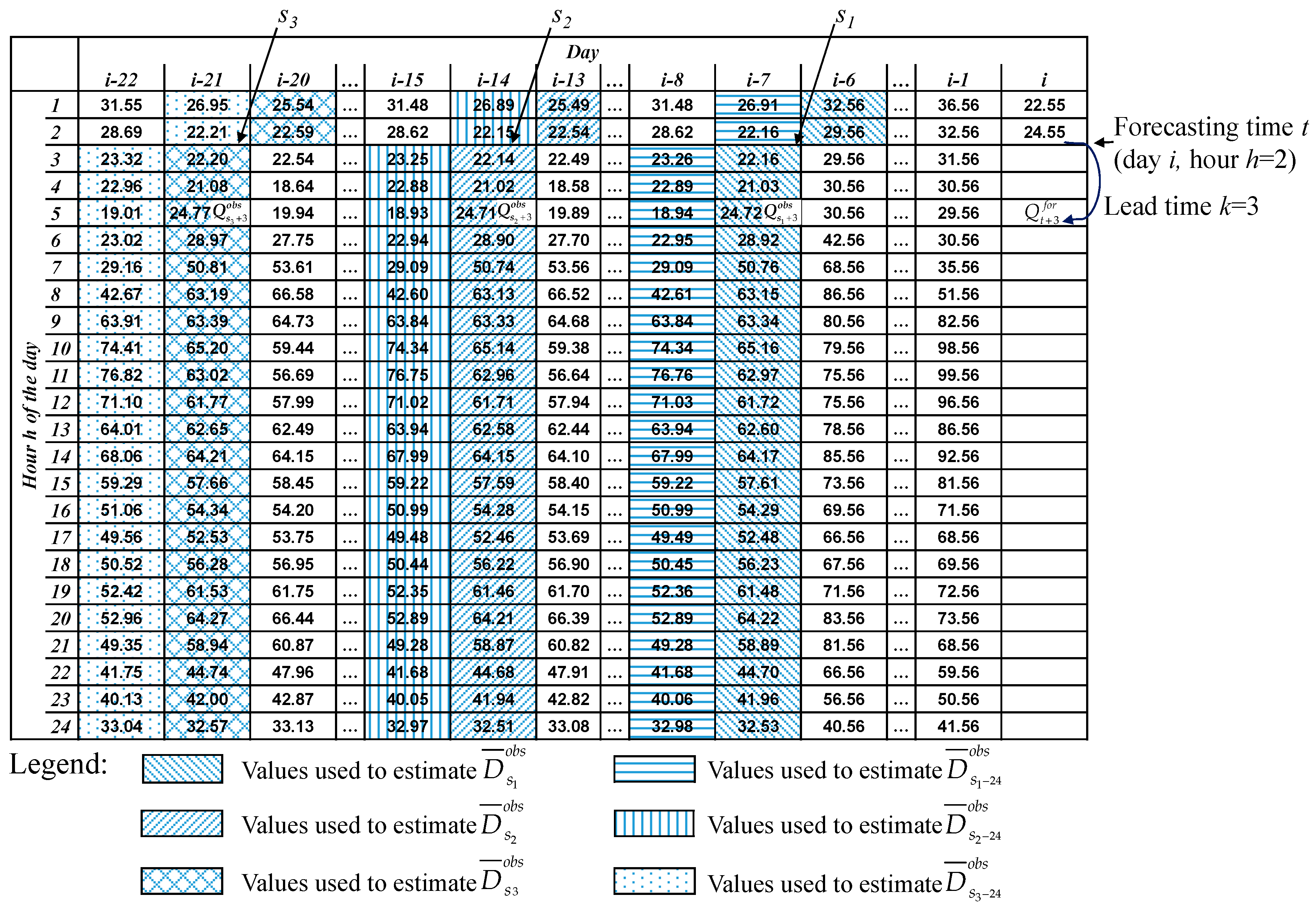
As is well known, hourly demands (i.e., average hourly water demands) are characterized by different patterns in the 7 days of the week and, with the exception of holidays, the days $\left\{i,i-7,i-14,i-21,..\right\}$ are of the same “type” (for example, they are all Tuesdays/weekdays). Therefore, once the forecasting time $t=24(i-1)+h$ (counted from the beginning of the year) has been established, it will be possible to identify the n hours that correspond to the same hour h of the day on which the forecast is made and belongs to the same “type” of day in the previous n weeks. The set S of these n hours can thus be defined as:

$$S=\left\{s_1;s_2;...;s_n\right\}=\left\{t-7\times 24;t-7\times 24\times 2;...;t-7\times 24\times n\right\}=\left\{t-168;t-336;...;t-168\times n\right\}$$

(4)

Within this framework, n can be interpreted as the length/extension of a moving window, that “moves” with t. It is important to clarify that the definition of the set S of n hours that corresponds to the same hour h of the day on which the forecast is made and belongs to the same “type” of day as provided in Equation (4) applies under “ordinary” conditions, that is, when the day considered is a Monday or a Tuesday or a Sunday and not a public holiday falling on a weekday. In the latter case, supposing for example that a holiday falls on a Tuesday, s₁, s₂,…, s_n would not be obtained by going back 7 × 24 h, 7 × 24 × 2 h,… 7 × 24 × n h, that is, by considering the Tuesdays of the previous weeks, but rather by selecting the corresponding hours of the previous Sundays (or other holidays, considered equivalent to Sundays). In the example considered, where the forecasting time t corresponds to an hour of a holiday falling on a Tuesday, s₁ would be equal to t − 2 × 24, therefore, going back 2 days, from Tuesday to Sunday, s₂ would be equal to t − (2 + 7) × 24, whilst considering the same hour occurring two Sundays ago, s₃ would be equal to t − (2 + 7 × 2) × 24, …, and s_n would be equal to t − (2 + 7 × (n − 1)) × 24. Incidentally, in this case, the series of observed data would be slightly shorter than n weeks (since s_n = t − (2 + 7 × (n − 1)) × 24, and not s_n = t − (7 × n) × 24 as in the case of an “ordinary” condition (see Equation (4)).

For the sake of simplicity, when referring to the set of n hours corresponding to the same hour h of the day on which the forecast is made and belonging to the same “type” of day, from this point on we will mean “ordinary” conditions and, thus, a moving window of n weeks preceding the forecasting time t. Clearly, if the forecasting time t corresponds to an hour of a holiday falling on a weekday, the moving window will be shorter than n weeks; conversely, if the forecasting time t corresponds to an hour of a weekday, but a holiday has fallen on the same type of weekday in the n previous weeks, that day cannot be included in the set S, making it necessary to lengthen the series by going back an additional week.

Having clarified these points, the coefficient ${\mathsf{\alpha }}_t$ can be estimated in the following manner:

$${\mathsf{\alpha }}_t=\frac{1}{n}{\displaystyle \sum _{s_j=s_1}^{s_n}\frac{{\overline{D}}_{s_j}^{obs}}{{\overline{D}}_{s_j-24}^{obs}}}$$

(5)

where ${\overline{D}}_{s_j}^{obs}$ is the observed average water demand in the 24 h following the hour s_j (with j = 1, 2, …, n) while, with reference to Equation (4) and under “ordinary” conditions, s₁ = t − 7 × 24, s₂ = t − 7 × 24 × 2,…, s_n = t − 7 × 24 × n, and ${\overline{D}}_{s_j-24}^{obs}$ is the observed average water demand in the 24 h preceding the hour s_j (i.e., from s_j − 24 to s_j) (see Figure 1).

The coefficient ${\mathsf{\beta }}_{t,k}$, related to the specific lead time k of the horizon of K = 24 h that begins at the time t, is estimated as follows:

$${\mathsf{\beta }}_{t,k}=\frac{1}{n}{\displaystyle \sum _{s_j=s_1}^{s_n}\frac{Q_{s_j+k}^{obs}}{{\overline{D}}_{s_j}^{obs}}}$$

(6)

where $Q_{s_j+k}^{obs}$ is the hourly water demand in the k-th hour following the hour s_j (with j = 1, 2, …, n). It should be noted that at every forecasting time step t, 24 values of the coefficient ${\mathsf{\beta }}_{t,k}$ are calculated, one for each forecast lead time k (with $k=1,2,...,K=24$). The earlier considerations regarding the definition of the set S where the forecasted hour corresponds to an hour of a holiday falling on a weekday clearly apply for the estimation of ${\mathsf{\beta }}_{t,k}$ as well.

A numerical example of estimation of the coefficients ${\mathsf{\alpha }}_t$ and ${\mathsf{\beta }}_{t,k}$ is provided in Appendix A.

2.2. Considerations on the Length n of the Moving Window

What has been illustrated above shows that the coefficients ${\mathsf{\alpha }}_t$ and ${\mathsf{\beta }}_{t,k}$ implicitly contain information characterizing the water demand of a certain “type” of day and a given hour of the day. However, these coefficients are continuously updated, being computed over a moving window of n weeks (under “ordinary” conditions) which ends at the forecasting time step t and moves forward with it. Clearly, the length of the set S used to estimate the coefficients must be sufficiently long, for example n > 2, in order to stabilize the estimate of the coefficients themselves and avoid fluctuations caused by a particular/anomalous demand observed at a certain time step. Yet at the same time, the set S, and hence the moving window, should not be too long, for example n < 10, i.e., not more than two/three months, so that seasonal fluctuations in demand can be taken into account in the coefficients. In the case of a very long window, for example 6 months or one year, an offsetting effect would occur, so that if the forecasting step t were to fall, for example, in the summer, the corresponding coefficients would be estimated also on the basis of the observed demand data for the winter period, thus precluding a correct characterization of seasonal fluctuations.

There is a further advantage of considering a fairly short moving window: since the model is based on the data of the moving window alone, from an operational standpoint, it is only necessary to have n weeks of observed water demand data in order to implement it. As seen in the introduction, unlike other models it does not require a long calibration dataset.

2.3. Model with Holidays and Special Occasions

The previously illustrated model, hereinafter referred to as the αβ_WDF (αβ Water Demand Forecasting) model, is structured assuming that public holidays and other special occasions can be considered like Sundays, although in the literature (e.g., Bakker et al., 2013) it has been observed that the water demand pattern associated with specific holidays is slightly different from the one typical of Sundays.

We can take account of this different pattern by slightly modifying the method of estimating the coefficients ${\mathsf{\beta }}_{t,k}$, though this implies the need to have m (with m ≥ 2) years of observed water demand data at our disposal.

Essentially, if the forecasted hour falls within a public holiday—being the average water demand ${\overline{D}}_t^{for}$ over the K = 24 h following the time t still estimated as provided in Equation (2), with ${\mathsf{\alpha }}_t$ estimated by means of Equation (5)—the hourly water demand $Q_{t+k}^{for}$ for the hour corresponding to t+ k (with $k=1,2,...,K=24$) can be estimated using Equation (3), but in this case the coefficients ${\mathsf{\beta }}_{t,k}$ will be estimated on the basis of the data recorded for the forecasted hour corresponding to t + k on the same holiday in the m previous years.

Practically speaking, therefore, in this case ${\mathsf{\beta }}_{t,k}$ is given by:

$${\mathsf{\beta }}_{t,k}=\frac{1}{m}{\displaystyle \sum _{s_y=s_1}^{s_m}\frac{Q_{s_y+k}^{obs}}{{\overline{D}}_{s_y}^{obs}}}$$

(7)

where s_y denotes the hour of the same holiday corresponding to the current time t but occurring y years earlier and hence $Q_{s_y+k}^{obs}$ is the hourly water demand corresponding to the observed forecasted hour (which falls within a holiday) y = 1, 2, …, m years earlier and ${\overline{D}}_{s_y}^{obs}$ is the corresponding average water demand observed in the 24 h following the hour s_y in the y = 1, 2,…, m previous years.

For the sake of brevity, this variant of the model αβ_WDF will hereinafter be referred to as αβ_h_WDF (αβ holiday Water Demand Forecasting) model.

3. Case Study

The proposed model was applied to the real-life case of Castelfranco Emilia (Italy). The water distribution system of Castelfranco Emilia serves about 23,000 inhabitants and is supplied by a tank equipped with a flow meter which provides a measurement of the water consumption of the entire town, including leakage. Hourly demand data are available for the years 1997, 1998, 1999, and 2000. Since an analysis revealed that data for various periods of the years 1997 and 1999 were either missing or unreliable, it was decided to use the years 1998 and 2000 for the purpose of applying and evaluating the effectiveness of the model.

The same data were used in a case study by [10], who undertook to apply and test a model they proposed called Patt_WDF (Pattern based Water Demand Forecasting). The results of the Patt_WDF model were thus used by way of comparison to analyze the effectiveness of the model here proposed. More specifically, the performance of the two models was assessed considering the 24 forecasting time horizons (i.e., the forecasts for 1, 2, and up to 24 h ahead) and using the Root Mean Square Error (RMSE) and Mean Absolute Error (MAE%) defined as:

$$\mathrm{RMSE}=\sqrt{\frac{1}{z}{\displaystyle \sum _{i=1}^z{e}_i^2}}$$

(8)

$$\mathrm{MAE}\%=\frac{1}{z}{\displaystyle \sum _{i=1}^z\left|\frac{e_i}{{\mu }_{obs}}\right|\times 100}$$

(9)

where z is the number of hours in the period considered (for example, a year), $e=Q^{obs}-Q^{for}$ is the error, $Q^{obs}$ is the value of the observed hourly water demand, $Q^{for}$ is the value of the forecasted hourly water demand, and ${\mathsf{\mu }}_{obs}$ is the mean of the observed values.

It should be noted that, as stated in the introduction, the Patt_WDF is a short-term water demand forecasting model based on a hybrid technique; like the αβ_WDF model, the Patt_WDF model is based on a 24-h time horizon and an hourly time step, but unlike the αβ_WDF model, the Patt_WDF model requires at least a year of observed water demand data for calibration purposes. In particular, as complete data were available for the years 1998 and 2000, the 1998 data and 2000 data were used for the calibration and validation, respectively, of the Patt_WDF model. Accordingly, though the αβ_WDF model does not require calibration periods in the strict sense, it was decided to present the results for the years 1998 and 2000 separately in order to enable a straightforward and meaningful comparison with the results of the Patt_WDF model.

More specifically, in the next section we start off by presenting an analysis of the results obtained with the αβ_WDF model, applied assuming n = 4, i.e., considering a moving window of observed data of 4 weeks under “ordinary” conditions for the estimation of ${\mathsf{\alpha }}_t$ and ${\mathsf{\beta }}_{t,k}$. These results are then compared with those of the Patt_WDF model. Subsequently, with specific reference to public holidays alone, a comparison between the results provided by the αβ_WDF model and those provided by the αβ_h_WDF model is presented; the coefficients ${\mathsf{\beta }}_{t,k}$ assumed when applying the latter were estimated on the basis of observed data for the years 1997 and 1999 as well (since data related to the holidays considered were also available for these years).

4. Analysis and Discussion of the Results

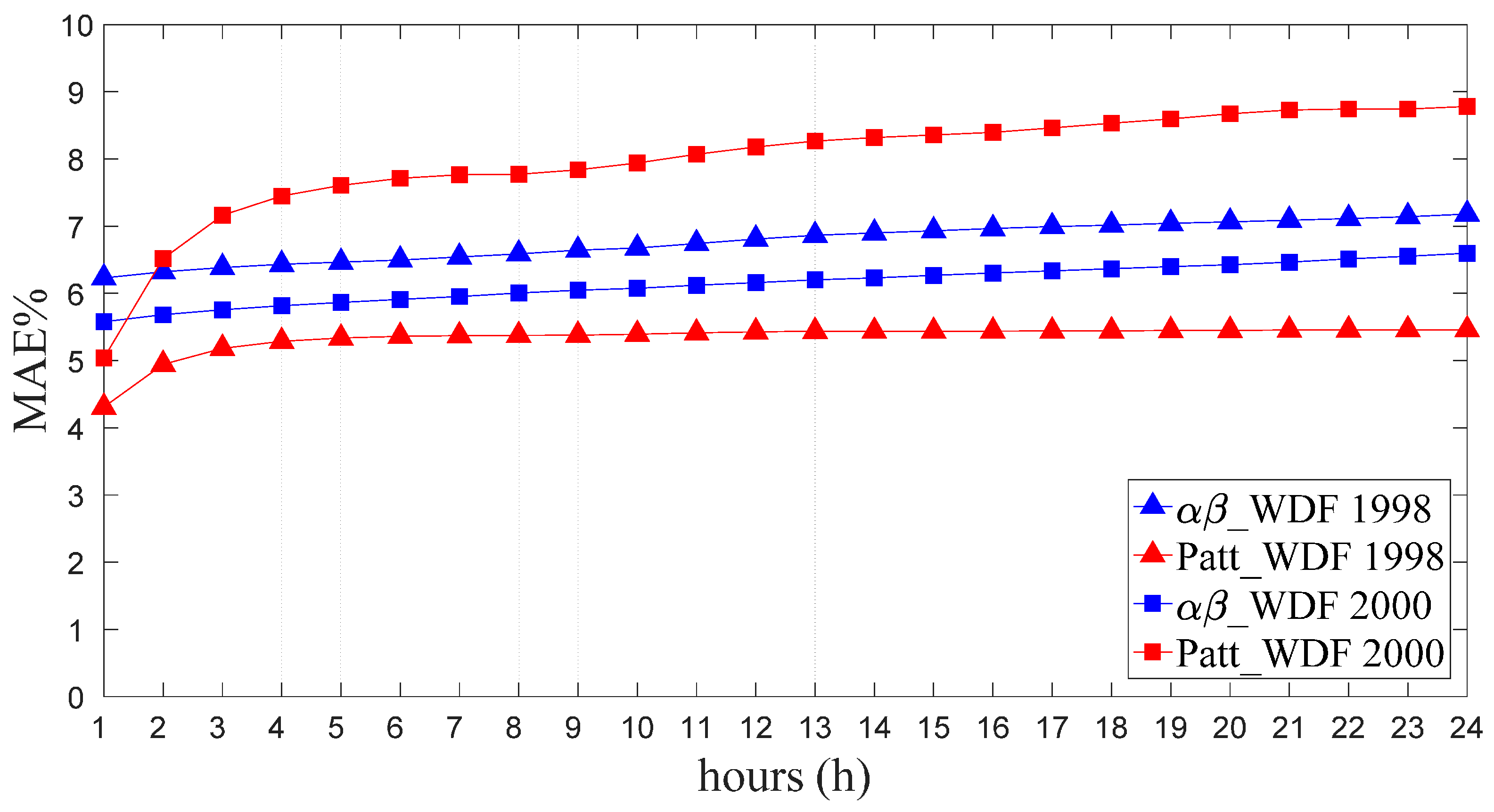
Figure 2 and Figure 3 show the RMSE and MAE% values for different forecasting time horizons, ranging between 1 and 24 h, for the years 1998 and 2000 obtained with the αβ_WDF model and the Patt_WDF model.

Based on an analysis of the results provided by the αβ_WDF model, it may be observed that the forecasting accuracy is in general very good, with RMSE values in the range of 4–6 L/s and corresponding MAE% values between 5% and 7%. More specifically, it can be observed that the accuracy is greater for short time horizons and decreases slightly with increases in the lead time, although the variations of the RMSE and MAE% remain, in any case, very modest. With reference to the model’s application to the year 1998, the RMSE increases from about 4.5 L/s for the 1-h-ahead forecast to about 5.5 L/s for the 24-h-ahead forecast and the MAE% rises accordingly from about 6% for the 1-h-ahead forecast to about 7% for the 24-h-ahead forecast. Similarly, when the model is applied to data for the year 2000, the RMSE increases from about 5.0 L/s for the 1-h-ahead forecast to about 6.0 L/s for the 24-h-ahead forecast and the MAE% increases from about 5.5% to about 6.5%. Incidentally, the fact that MAE% is generally lower in 2000 than that observed in 1998, while for RMSE the reverse applies, is due to the fact that in 2000 the average hourly water demand had a slight increment and, at the same time, the magnitude of the errors is almost the same (see Equation (9)).

A comparison of the results provided, respectively, by the αβ_WDF model and Patt_WDF model shows that when the models were applied to data for the year 1998 (calibration period for the Patt_WDF model), the Patt_WDF model provided better forecasting accuracy than the αβ_WDF model for all time horizons, with RMSE values ranging from about 3 L/s for the 1-h-ahead forecast to about 4 L/s for the 24-h-ahead forecast and MAE% values ranging from about 4.5% for the 1-h-ahead forecast to about 5.5% for the 24-h-ahead forecast. Conversely, when the models were applied to data for the year 2000 (validation period for Patt_WDF), the αβ_WDF model generally provided better accuracy. The two models showed a similar RMSE for the 1-h-ahead forecast (4.5 L/s in the case of the Patt_WDF model and 5 L/s in the case of the αβ_WDF model), but the performance of the αβ_WDF model was better for other time horizons; specifically, the RMSE for the 24-h-ahead forecast was greater than 7 L/s in the case of the Patt_WDF model versus 6 L/s for the αβ_WDF model (corresponding to an MAE% of about 9% in the case of the Patt_WDF model and 6.5% for the αβ_WDF model). In general, comparing the trends in the indexes resulting from the two models when applied to two different years of data, it can be observed that the performance of the αβ_WDF model did not vary significantly from year to year, whereas that of the Patt_WDF model was significantly worse when applied to the 2000 data as opposed to the 1998 data. This is understandable, considering that the Patt_WDF model, unlike the αβ_WDF model, requires a set of calibration data regarding a long period (1 year). The Patt_WDF model is thus able to deliver high forecasting accuracy in relation, precisely, to the 1998 calibration data, i.e., the dataset used to characterize the periodic patterns on which the forecasting model is based. However, switching to another year (validation), and hence a different dataset, the model’s performance tends to decline. In contrast, the performance of the αβ_WDF model remains stable from one year to another, as it does not require a long calibration dataset and its forecasts are made using coefficients that are continuously updated on the basis of a moving window.

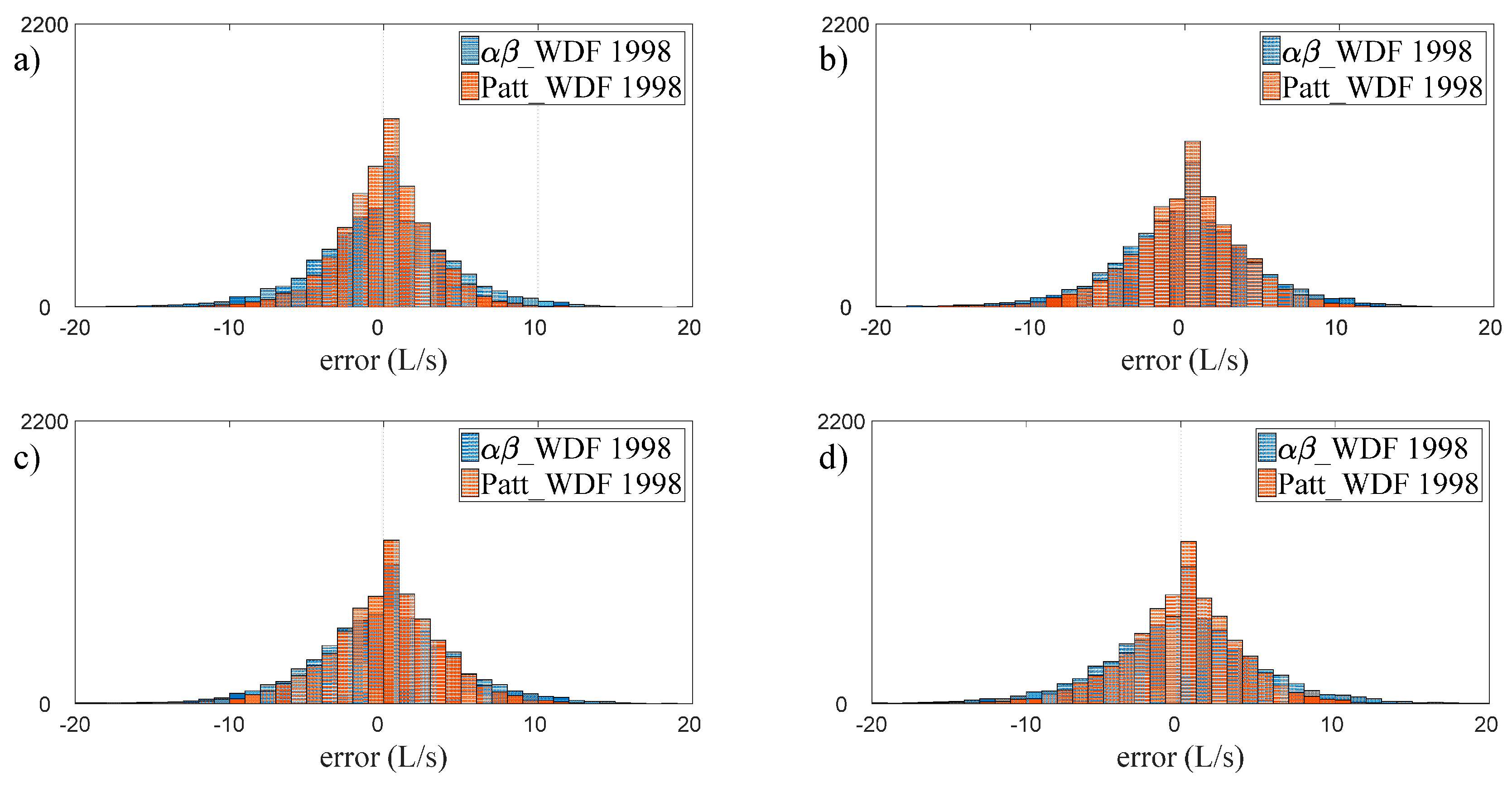
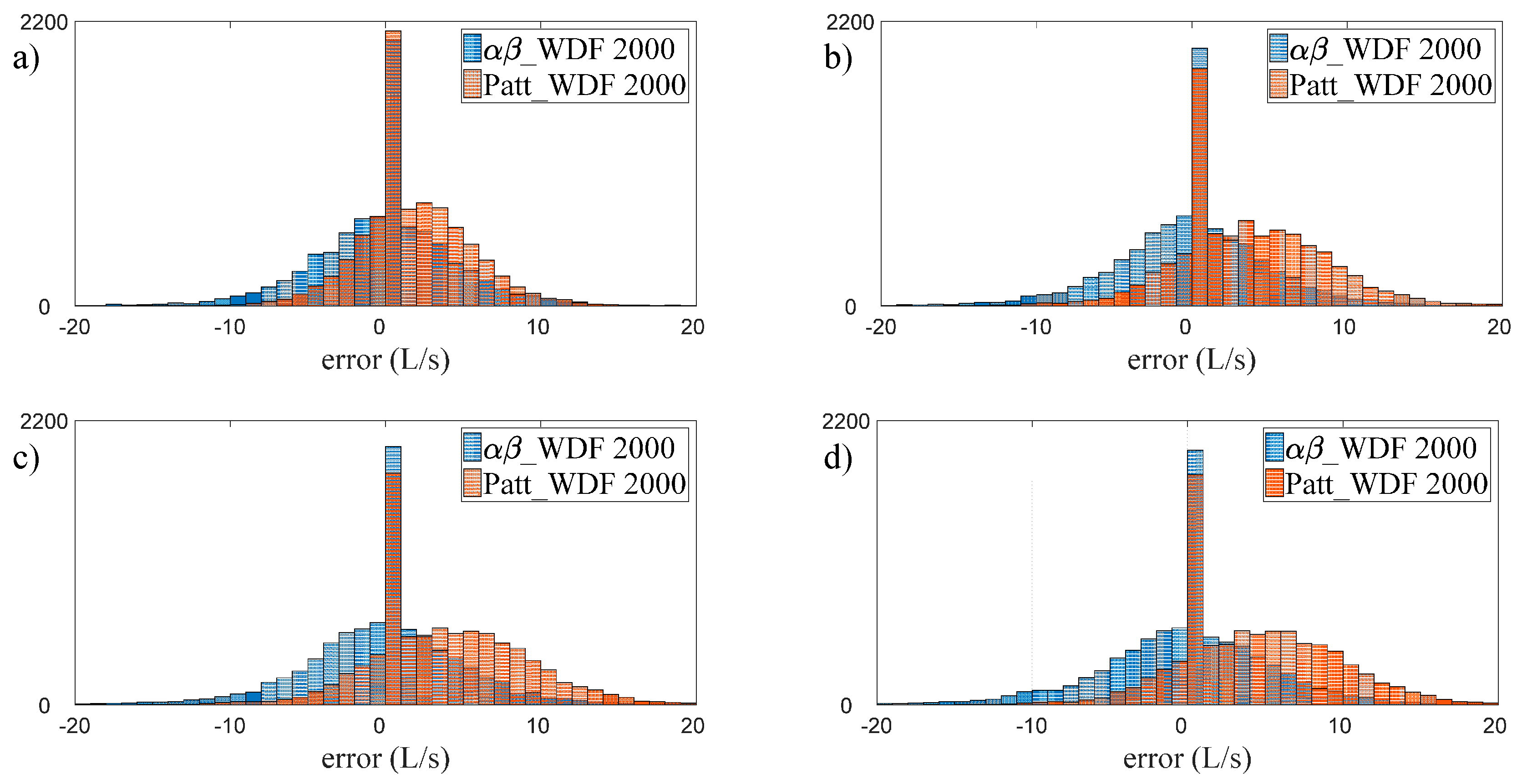
This different behavior of the two models is also confirmed by an analysis of the error frequency histograms shown in Figure 4 and Figure 5 for the years 1998 and 2000, respectively. In particular, in each figure, the histograms of the errors given by the two models in the 1-h-ahead (Figure 4a for 1998 and Figure 5a for 2000), 6-h-ahead (Figure 4b and Figure 5b), 12-h-ahead (Figure 4c and Figure 5c), and 24-h-ahead (Figure 4d and Figure 5d) forecasts are overlaid. Based on an analysis of Figure 4, relating to the year 1998, it may be noted, in general, that the histograms of the two models show wholly similar widths for the different time horizons considered and are centered on zero. More specifically, a slightly larger spread can be observed in the errors of the αβ_WDF model, confirming the better performance of the Patt_WDF model with respect to the (its) calibration period. However, analyzing the errors relating to the year 2000 (Figure 5), it can be observed that whilst the αβ_WDF model provides a symmetrical distribution of errors centered on zero, similar to one seen for 1998, the error distribution produced by Patt_WDF is not symmetric relative to zero, but is, rather, shifted onto the positive axis. This particular error distribution of the Patt_WDF model in the year 2000 indicates a general underestimation in the water demand forecast related to the validation period (the error being defined as $e=Q^{obs}-Q^{for}$). This is understandable, considering that the observed data for 2000 show a slight increase in water demands compared to 1998. When used to forecast the water demands of 2000, the Patt_WDF model, calibrated on the basis of the 1998 data, tends to underestimate them. This problem does not occur with the αβ_WDF model, since it does not rely on parameters calibrated over a specific year, but rather uses information deduced from the demands observed in the last n = 4 weeks and is thus capable of adapting to long-term variations in the demands themselves.

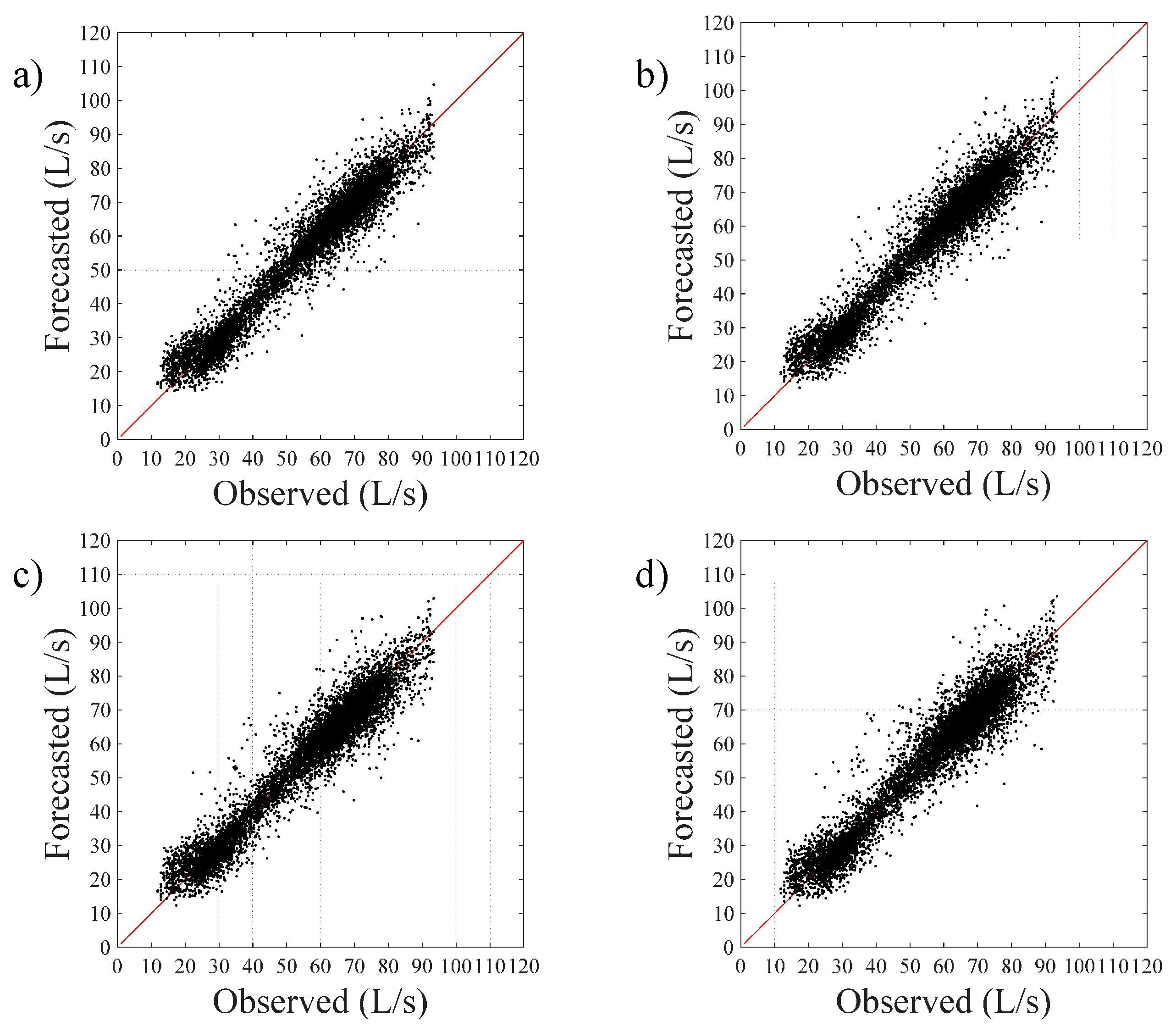
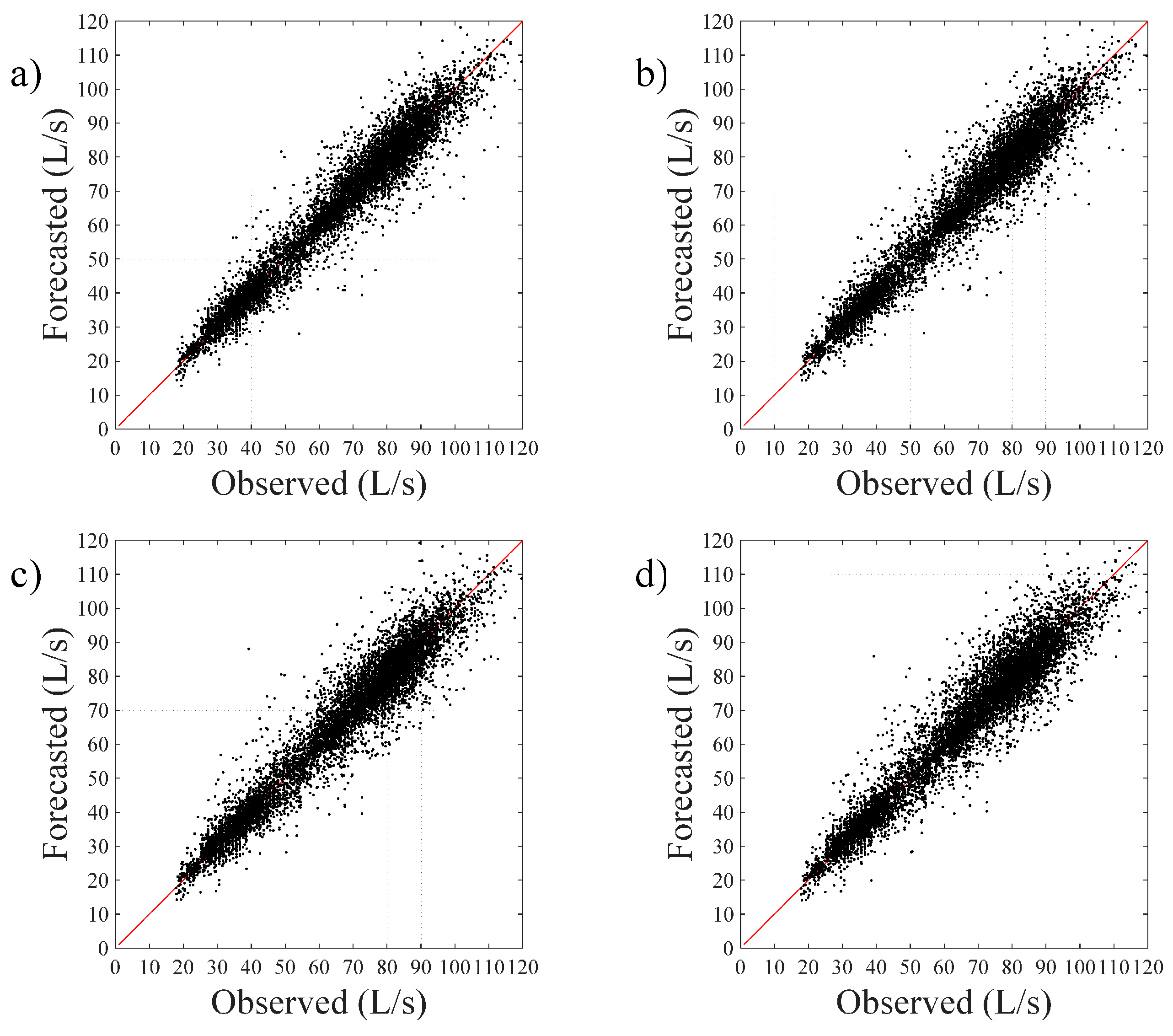
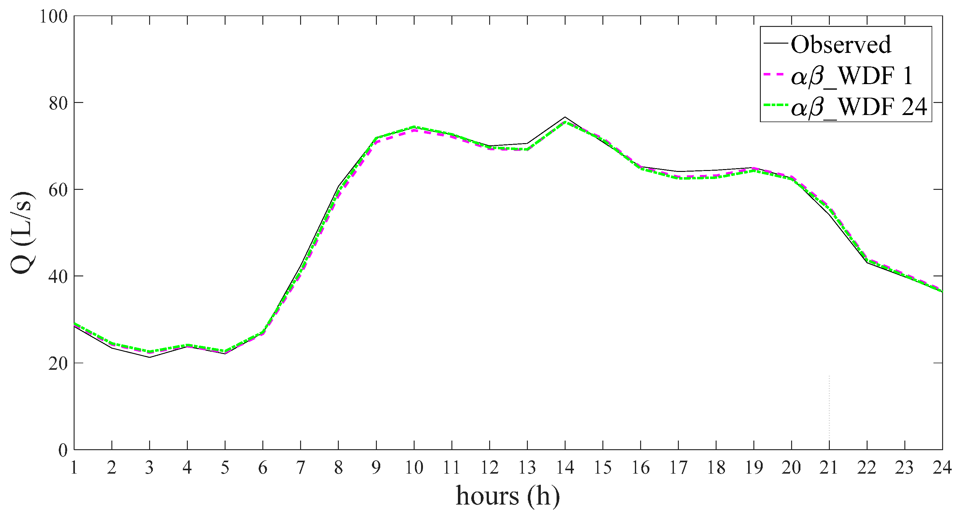
To conclude the analysis of the performance of the αβ_WDF model, in Figure 6 and Figure 7, scatter plots of the 1-, 6-, 12-, and 24-h ahead demand forecasts for the years 1998 and 2000, respectively are shown. Furthermore, in Figure 8, by way of example, a comparison between the observed water demand pattern for a generic day of the year 2000 (23 January) and the 1- and 24-h-ahead forecasts provided by the αβ_WDF model is shown. The scatter plots in Figure 6 and Figure 7 confirm the accuracy of the forecast provided by the αβ_WDF model, as all of the points are distributed around the 45° line, which represents a perfect correspondence between observed and forecasted demands, and the forecasting accuracy remains practically constant as the time horizon changes (from 1 to 24 h): no significant variation can be noted in the width of the cloud of points, either for the year 1998 or the year 2000. The comparison in Figure 8 likewise shows that the trend in water demand predicted in the 1- and 24-h-ahead forecasts of the αβ_WDF model very closely approximate the historically observed demands.

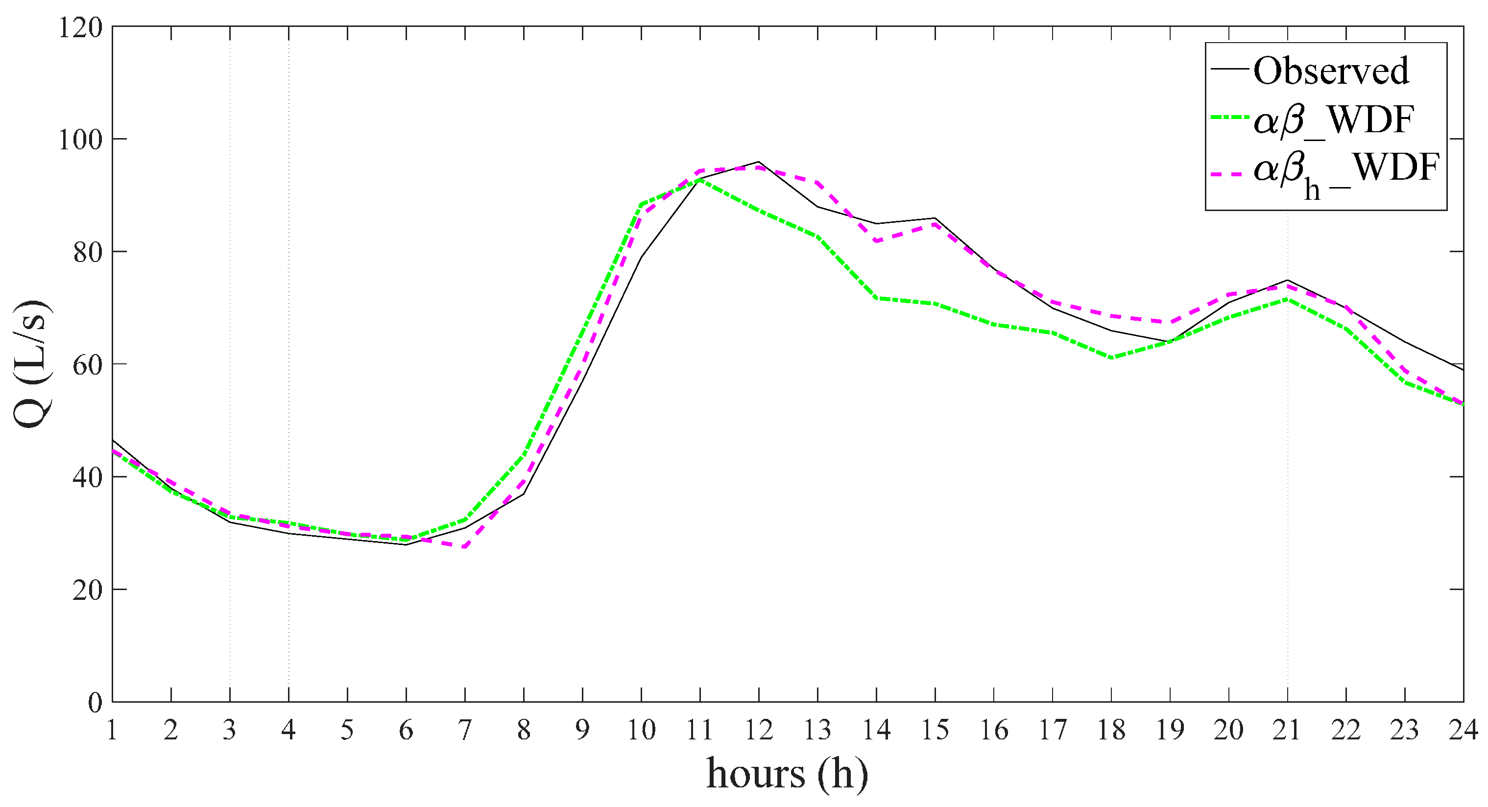
Finally, we shall now focus our attention on the days corresponding to public holidays or special occasions.

Figure 9 shows, by way of example, the pattern of observed water demands on one holiday in the year 2000, the 1st of May (international workers’ day) and the corresponding 1-h-ahead forecast provided by the αβ_WDF model. It is evident that the forecast provided by the αβ_WDF model for this holiday is less accurate than the one shown in Figure 8, which relates to a generic weekday. More generally speaking, considering all and only the holidays falling in a year (for a total of about ten), the greater difficulty in correctly predicting demands is confirmed by the RMSE and MAE% values, which tend to be higher. In fact, considering only the holidays in the year 2000, the RMSE takes on values in the range of 8.5 to 10 L/s, respectively, for the 1- and 24-h-ahead forecasts, corresponding to MAE% values of between 10% and 13%, versus RMSE values of about 5 and 6 L/s, corresponding to MAE% values of 5.5% and 6.5%, when all the days of the year 2000 are considered.

With respect to these particular types of days, the application of the αβ_h_WDF model can provide a benefit. Indeed, as can be observed in Figure 9, which also shows the 1-h-ahead forecast provided by the αβ_h_WDF model, the estimate of the coefficients ${\mathsf{\beta }}_{t,k}$ made for the same holiday in the m = 3 previous years (1997, 1998, and 1999) (see Equation (7)) enables a more accurate forecast of the trend in water demand. This is further confirmed by the RMSE and MAE% values computed considering all and solely the public holidays in the year 2000, as they fall slightly from 8.5 and 10 L/s, respectively, for the 1- and 24-h-ahead forecasts of the αβ_WDF model—corresponding to MAE% values in the range of 10% to 13%—to 7.5 L/s and 8 L/s, respectively, for the 1- and 24-h-ahead forecasts of the αβ_h_WDF model, corresponding to MAE% values in the range of 9.5% to 10%.

5. Conclusions

In this article a new model for forecasting short-term demands in a water distribution system has been proposed. The model provides a forecast for the following 24 h using a pair of coefficients whose value is updated at every forecasting step on the basis of (a) the observed demand data pertaining to the 24 h prior to the time the forecast is made and (b) the observed data pertaining to several previous weeks for the same type of day and the same hour of the day falling within the forecasting interval. Application of the model to a real-life case and a comparison with the results provided by another short-term forecasting model based on the representation of periodic water demand patterns have revealed that the proposed αβ_WDF model has a good predictive capability over the entire forecasting time horizon considered (24 h); furthermore, it does not require calibration periods in the strict sense, being based solely on the water demands observed in the few weeks prior to the time at which the forecast is made. From an operational standpoint, this means that in cases in which long historical series of observed data are not available, the model can be used 1 or 2 months after data collection begins. Finally, again by virtue of the fact that the model does not require a static calibration of parameters, since the parameters are updated as time passes, the forecasting accuracy remains constant and high when applied to different years and/or periods. The values of the performance indicators (RMSE and MAE%) were distinctly better for the αβ_WDF model than for the pattern-based model it was compared to, which requires calibration on the basis of at least one year of data, when the comparison was made with reference to a period other than the one used for the latter model’s calibration.

Finally, it was observed that the forecasting accuracy provided by the proposed αβ_WDF model tends not to be as good when evaluated in relation to certain public holidays falling in the year; in these cases, if information is available about water demands observed during the same holidays in several previous years, the application of a variant of the model, referred to as αβ_h_WDF, enables a certain improvement in forecasting accuracy. In conclusion, its good forecasting capability over different time horizons and different periods/years, combined with the need for a small set of observed data for its implementation, make the proposed model a robust and effective water demand forecasting tool to be used in the context of real-time network management, potentially for any network size. This is due to its nature which is based on the use of data observed just prior to the time of the forecast. However, this latter aspect is currently under investigation considering case studies different from the one here examined, which regards a middle size pipe network, in order to characterize its efficacy as the number of served users changes. Results will be published in due time.