Observations and Prediction of Recovered Quality of Desalinated Seawater in the Strategic ASR Project in Liwa, Abu Dhabi

Abstract

To be able to overcome water shortages, Abu Dhabi Emirate started an Aquifer Storage and Recovery (ASR) project with desalinated seawater (DSW) as source water near Liwa. It is the largest DSW-ASR project in the world (stored volume ~10 Mm³/year), and should recover potable water for direct use. DSW is infiltrated into a desert dune sand aquifer using “sand-covered gravel-bed” recharge basins. In this study, we evaluate the hydrogeological and hydrogeochemical stratification of the (sub)oxic target aquifer, and water quality changes of DSW during trial infiltration runs. We predict water quality changes of DSW after 824 d of infiltration, during 90 d of intensive recovery (67% recovered) without storage (scenario A), as well as after 10 years of storage (scenario B, with significant bubble drift). Monitoring of preceding trials revealed a lack of redox reactions; little carbonate dissolution and Ca/Na exchange; much SiO₂ dissolution; a strong mobilization of natural AsO₄³⁻, B, Ba, F, CrO₄²⁻, Mo, Sr and V from the (sub)oxic aquifer; and immobilization of PO₄, Al, Cu, Fe and Ni from DSW. The Easy-Leacher model was applied in forward and reverse mode including lateral bubble drift, to predict water quality of the recovered water. We show that hydrogeochemical modeling of a complex ASR-system can be relatively easy and straightforward, if aquifer reactivity is low and redox reactions can be ignored. The pilot observations and modeling results demonstrate that in scenario A recovered water quality still complies with Abu Dhabi’s drinking water standards (even up to 85% recovery). For scenario B, however, the recovery efficiency declines to 60% after which various drinking water standards are exceeded, especially the one for chromium.

1. Introduction

Water scarcity has driven many countries in arid zones, such as the Middle East and Abu Dhabi in particular, to desalinate large volumes of seawater for fresh water supply [1]. Episodic problems with seawater quality due to, e.g., harmful algae blooms [2,3] and oil spills, energy supply and fear of war or terrorism have nurtured the urgent need to store desalinated seawater in the underground for later use in case of a calamity [4,5,6,7].

In 2001, Abu Dhabi started its pioneer projects for developing strategic fresh water resources to face any emergency condition using the Aquifer Storage and Recovery (ASR) technique by infiltrating the surplus of desalinated water into the groundwater aquifer system. One of these projects is the strategic fresh water reserve project at Liwa. The project passed with success through the phases of first a feasibility study and subsequently a pilot study in 2003–2004 [8]. In this pilot, desalinated water was infiltrated in a dune sand aquifer system using injection wells as well as an underground recharge basin. The basin performed better than the ASR wells, and was therefore selected for implementation in the construction phase.

Construction of the full ASR plant started in 2009, and was finalized in Winter 2016. Large scale infiltration started in May 2015. The project aim is to infiltrate 26,500 m³/d (=9.7 Mm³/year) of desalinated water with Total Dissolved Solids (TDS) < 250 ppm for 824 d, in order to be able to cover an emergency water demand for 90 d with a recovery rate of 170,280 m³/d (=15.5 Mm³/90 d) and a TDS of ~400 ppm.

After extensive studies on the ASR recovery efficiency (the part of injected water that can be recovered with a satisfying quality), impact on groundwater tables and salinity distribution, and quality of the water to be recovered [8,9,10,11,12], questions persisted about a potential water quality deterioration during recovery after a prolonged storage period, with emphasis on critical Cr(VI) behavior. This related to the planned omission of a post-treatment of the recovered water, which was to be distributed directly without any treatment, as drinking water to Abu Dhabi City, trusting that the UAE drinking water standards [13] would not be exceeded. It was feared, however, in a late stage, that post-treatment would be needed requiring a costly facility, for two reasons. Firstly, the native groundwater in the project area contains elevated concentrations of, among others, TDS, Cl, SO₄, F, Na and Cr (as CrO₄²⁻), exceeding the standards, suggesting that their mobilization would deteriorate water quality during prolonged storage. Secondly, water stored in ASR targeted aquifers generally displays significant quality changes due to redox reactions, cation exchange, desorption and dissolution of mineral phases [14,15,16,17,18,19,20,21,22].

In order to assess the impact of aquifer storage on the recovered water quality, we first investigated the hydrogeological, geochemical and hydrochemical stratification of the targeted aquifer system, based on available data [8,9,10,11,12]. We conducted a sampling campaign in the period of 3–7 August 2014 to check potential bias in the existing hydrochemical data set, and to obtain data on chromium speciation (Cr(III) versus Cr(VI)). Finally, we predicted the future quality of the recovered DSW after 27 months of infiltration, during 90 d of intensive recovery without storage, as well as after 10 years of storage (with significant lateral bubble migration).

This paper is based on two extensive reports [23,24]. It shows the peculiar characteristics of an eolian-fluvial sand (stone) aquifer system in a desert environment, the unique water quality changes during an ASR pilot including a six-year storage phase, and a particular modeling approach. In this approach, observations on retardation and leaching are combined with a strong schematization of the complex ASR system, flow, and processes.

2. Materials and Methods

2.1. Field Site and Liwa ASR System

The project area (Figure 1, Figure 2 and Figure 3) is situated in a remote dune sand area ~150 km southwest of Abu Dhabi City, some 25 km north of the Liwa Crescent (Al Qafa area). Its hydrological position is on or close to the phreatic groundwater divide of one of the few fresh groundwater reserves (Figure 2). The altitude of land surface varies between 120 and 160 m ASL (Above Sea Level).

The pilot area is ~15 km to the east of the final Liwa ASR plant (Figure 3). The plant is composed of three underground basins A–C (Figure 3), each with 105 surrounding recovery wells, and 57 monitoring wells in total. The circular recharge basins A, B and C, 50 m in diameter, are composed of a flat gravel-body covered by geo-textile and a sand layer on top, fed by horizontal reverse drains.

The ASR plant is thus not a normal ASR system, which is exclusively composed of wells performing two tasks: infiltrate and recover [20].

2.2. The Pilot

The first operation run of the pilot started on 1 October 2003 and lasted until December 2004. DSW was infiltrated via a series of 5 ASR wells (not discussed further) and a recharge basin recovery scheme consisting of a covered gravel-body with reverse drains in it, 4 recovery wells and tens of observation wells around. DSW was infiltrated via the basin for 250 d at ~250 m³/h, and after 48 d of storage part of the stored volume was recovered in 70 d at ~250 m³/h. Intensive monitoring of water quality yielded important insights in the ambient hydrochemical stratification and water quality changes during infiltration, stand-still and recovery [8].

A second infiltration run via the basin took place in 2008, but water quality monitoring was not undertaken and DSW was not pumped out. This offered the possibility to sample, in August 2014, 6-year-old DSW from the aquifer.

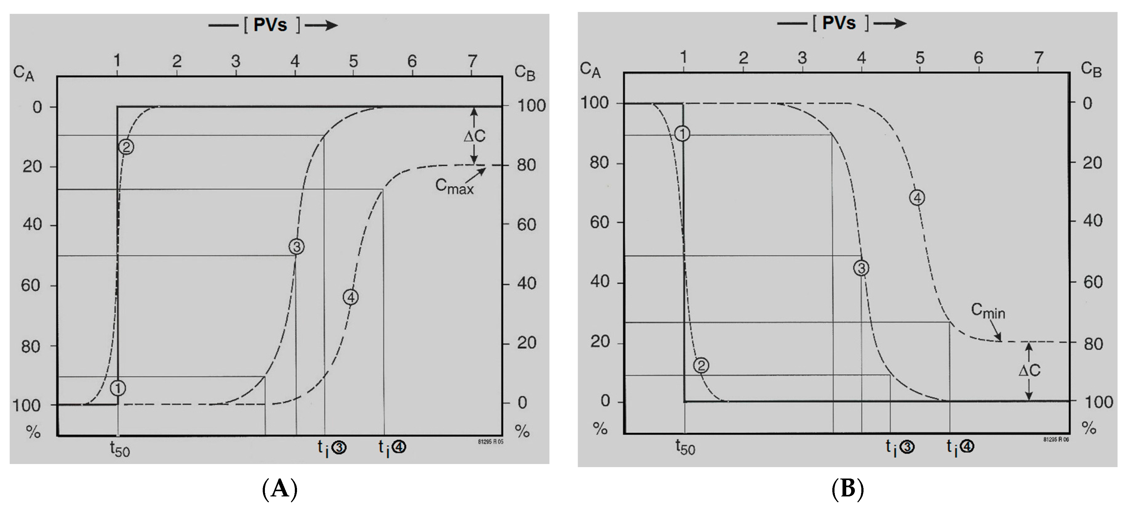
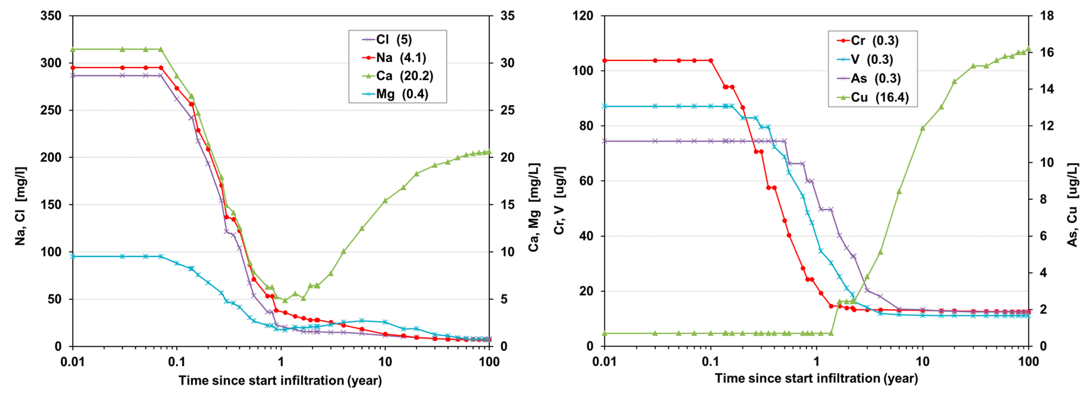
2.3. Quantitative Description of the Break-through Curve

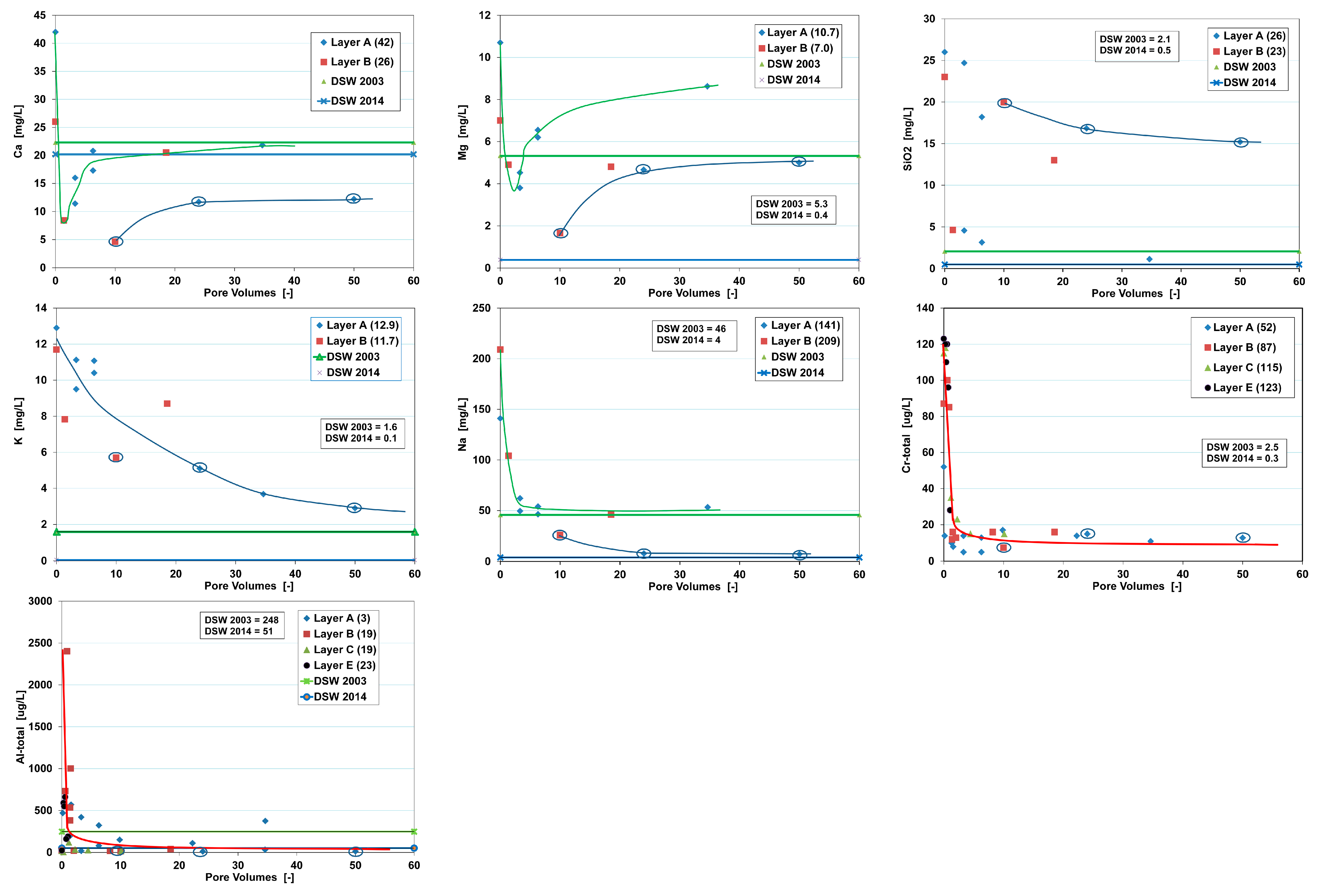
The first infiltration run of the pilot yielded valuable insight into the break-through curve (BTC) of nearly all main constituents and trace elements. These observed BTCs are characterized by 3 parameters: pore volume, retardation or leach factor and (semi)permanent concentration change (Figure 4).

The dimensionless parameter called “pore volume” (PV) forms the time axis of water quality observations and model predictions:

$$PV=\frac{t_{INF}}{t_{50}}$$

(1)

where t_INF = total infiltration period [d]; and t₅₀ = the observed 50% breakthrough time of conservative tracer or the calculated travel time via Equation (4).

One PV means that the whole aquifer, from infiltration point to the monitoring or recovery well, has been flushed with the infiltration water exactly one time. Retardation factors R or leach factors L can then be simply deduced from concentration plots against PVs (Figure 4).

Sorbing and oxidizing solutes as well as desorbing and dissolving solutes are retarded during aquifer passage compared with conservative solutes. In the latter case, raised concentrations drop to the influent level long after passage of the conservative chloride front. These delays are quantified for solute i by, respectively, the well-known retardation factor R_i, and the less well known leach factor L_i [25]:

$$R_i=\frac{t_i}{t_{50}}=1+\frac{{\rho }_S\left(1-n\right)K_d}{n}$$

(2)

$$L_i=\frac{t_i}{t_{50}}=1+\frac{{\rho }_S\left(1-n\right)\left(solid\right)}{n \left(reac\right) r_R}=1+\frac{{\rho }_S\left(1-n\right)\left(solid\right)}{n \left(prod\right) r_P}$$

(3)

where t_i = time required for ≥90% break-through (R_i) or ≥90% leaching (L_i) or till equilibrium is attained with the infiltration water [days]; ρ_s = density of solids of porous medium [kg/L]; n = porosity [L/L]; K_d = distribution coefficient (slope of the linear portion of the adsorption isotherm) [L/kg]; (solid) = content of reactive phase in aquifer [mmol/kg dry weight]; (reac) = concentration of reactant in flushing fluid [mmol/L]; (prod) = concentration of reaction product in fluid during leaching [mmol/L]; r_R = reaction coefficient, i.e., the number of mmoles of solid phase which is leached by 1 mmole of reactant [-]; and r_P = reaction coefficient related to (prod).

For practical reasons, t_i is set at ≥90% not at 100%. If for some reason, the BTC shows a partial breakthrough due to a prolonged phase of continued partial immobilization or mobilization, so the additional parameter ΔC is needed to describe the BTC (Figure 4). Equations (2) and (3) hold for a stationary retardation or leaching process, with a homogeneously distributed reactive phase in the aquifer. Of course, (reac) or (prod) should have no other sinks or sources, unless these can be properly accounted for.

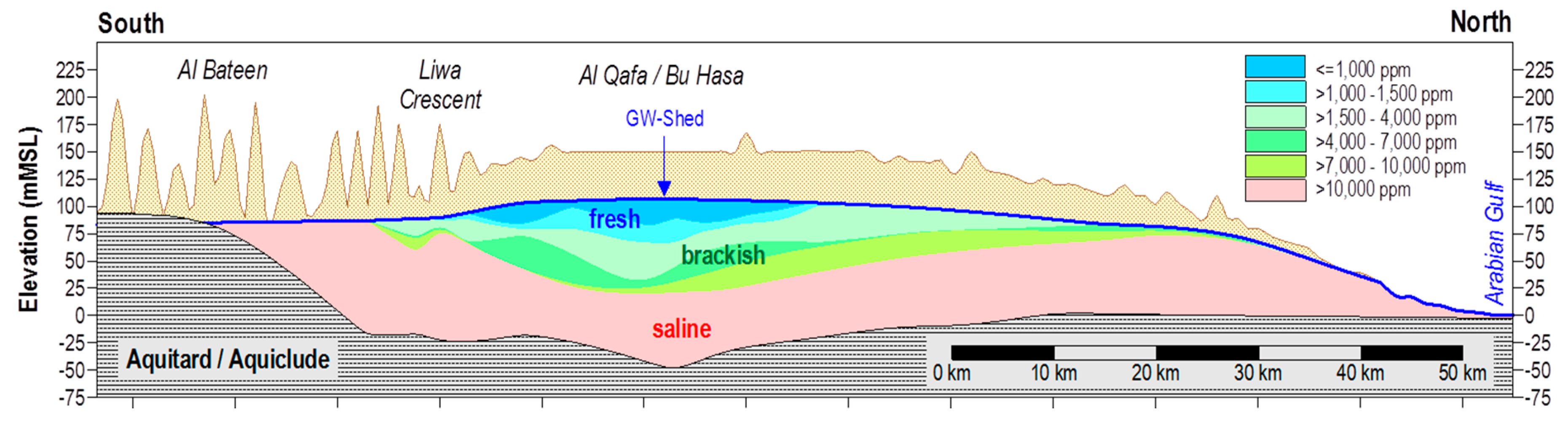
2.4. Lithological and Geochemical Stratification

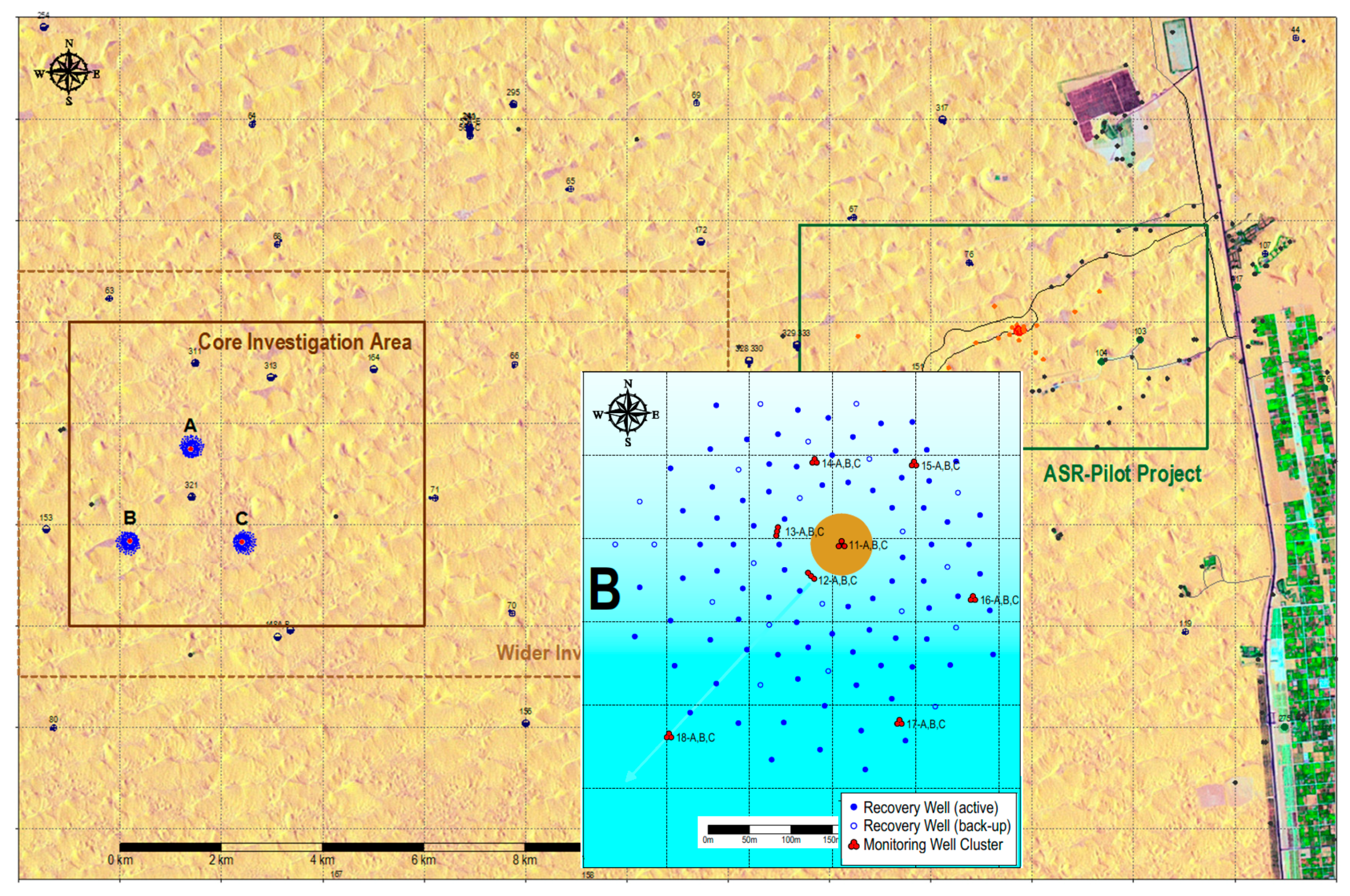
The aquifer system on well fields A, B and C could be schematized into a succession of 14 (sub) horizontal layers in between ground surface and 40 m below sea level [23], based on all drilling logs (>372), geophysical logs (including the eccentered wireline NMR logging of permeability and porosity), pumping tests, infiltration pilot tests and fluid flow logging, as presented by [9,10,11,12]. For modeling purposes, the 14 layers were aggregated into 6 main aquifer layers (a–f in Figure 5), of which the very low permeability aquitard f needs less consideration.

The mean geochemical composition of layers a–f was calculated from the geochemical data of 4 deep core drillings, one in each well field and one in the middle of well fields A, B and C. The data were derived from [12], containing the following information: Sample description with photographs, petrographic analysis and mineralogical counting by petrological photomicroscopic examination of a thin section impregnated with fluorescent resin, XRD analysis, porosimetric analysis, chemical analysis of main constituents (including LOI and Acid Solubility), chemical analysis of heavy metals (probably in nitric acid; no details given), and particle size distribution (by sieving).

The digital data of all 41 samples were used to calculate mean values for aquifer layers a–f, and to quantify the content of selected minerals by petrochemical calculations [23]. Petrochemical calculations were needed to correct specific data for water losses (loss on ignition), to calculate the cation exchange capacity (CEC) and to derive the mineral content from data on elements that are present in more than one mineral.

2.5. Hydrochemical Analyses in Period 2003–2013

Samples were taken from practically all recovery and monitoring wells, in both the pilot area and well fields A, B and C. The analyses include data on gases (O₂, residual Cl₂), turbidity, color, temperature, pH, EC, ORP (Oxidation Reduction Potential, Eh), main anions (Cl, SO₄, S, HCO₃, CO₃, NO₃, NO₂, PO₄, and F), main cations (Na, K, Ca, Mg, NH₄, Fe, and Mn), SiO₂, TOC (Total Organic Carbon), CN, selected trace elements (Ag, Al, As, B, Ba, Br, Cd, Cr, Cu, Hg, Mo, Ni, Pb, Sb, Se, Sr, V and Zn), and the stable isotopes ²H and ¹⁸O. Most samples were filtered in the field, and all concentrations (TOC excluded) refer to total dissolved concentrations, thus without (further) speciation. Microbial parameters and organic micropollutants were analyzed but showed negligible concentration levels.

Samples of the ambient groundwater were taken in the pilot area in 2003, and within and around well fields A, B and C in 2011–2013. Analytical data of DSW samples prior to infiltration, during and after aquifer passage were exclusively available from the pilot. All data (obtained from [9,10,11,12] and from data files supplied by Dr. G. Koziorowski (GTZ International Services) were controlled, elaborated and stored with Hydrogeochemcal.xlsx [26].

2.6. Monitoring Campaign in August 2014

In the period of 3–7 August 2014 a sampling campaign was conducted to take 31 samples from divergent observation wells that had been sampled earlier and from DSW, in order to: (i) check potential bias in the existing hydrochemical data set of well fields A, B and C; and (ii) obtain data on chromium speciation: Cr(III) versus Cr(VI).

Important aspects that were tackled with great care, are: sufficient well purging based on purged volume and stable field parameters, sampling without applying vacuum and excluding atmospheric exposition, reducing exposure to sunlight and wind, flow regulation of the pump, field measurements (EC, pH, temp, O₂), filtration of water over a 0.45 μm membrane, dedicated sample preservation for specific parameter groups, cooling, nearly daily shipment to the Netherlands, and rapid analysis in the certified Vitens Laboratory (Leeuwarden). The quality of the analysis was validated using HGC 2.0 to exclude potential impact of errors.

2.7. Predictions by EL Modeling

Two models were constructed, an Excel based Easy-Leacher (EL) model [25] and a PHREEQC-2 [27] flowtube model.

PHREEQC-2 was applied to model more in detail the behavior of chromate and arsenate along a small number of flowlines during infiltration phase. PHREEQC-2 and EL produced nearly identical results for chromate and arsenate behavior during infiltration, justifying the application of the simpler EL model. Further details about the PHREEQC-2 modeling and its results are given by [24] and not considered here further.

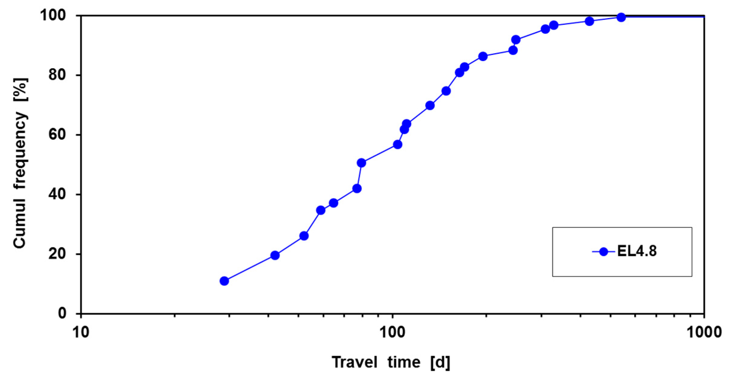
EL simplifies 3D groundwater flow into a 2D set of maximum 50 flow tubes through a maximum of 10 horizontal aquifer layers. The travel times are either derived from a hydrological model, or calculated analytically. Chemical transport is calculated on the basis of pore volumes (dimensionless time scale), retardation and leach factors (superimposed on the pore volumes) based on either mass balances or field observations, CaCO₃ equilibrium (if relevant), redox reactions (if relevant), and expert rules on among others redox reaction kinetics.

EL was given the task to do the all-round water quality modeling during all ASR phases (infiltration, storage with bubble drift, and recovery), and to combine the output of a relatively high number of flowlines into a mixed output as generated by a well field.

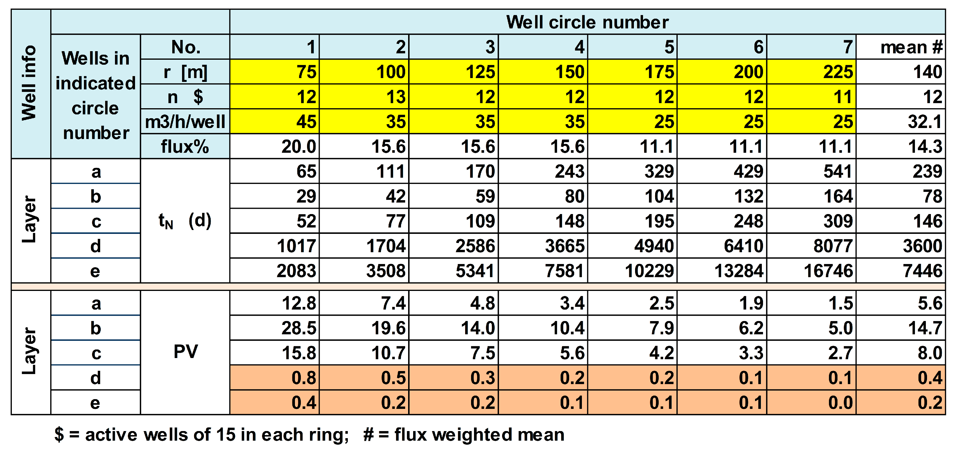
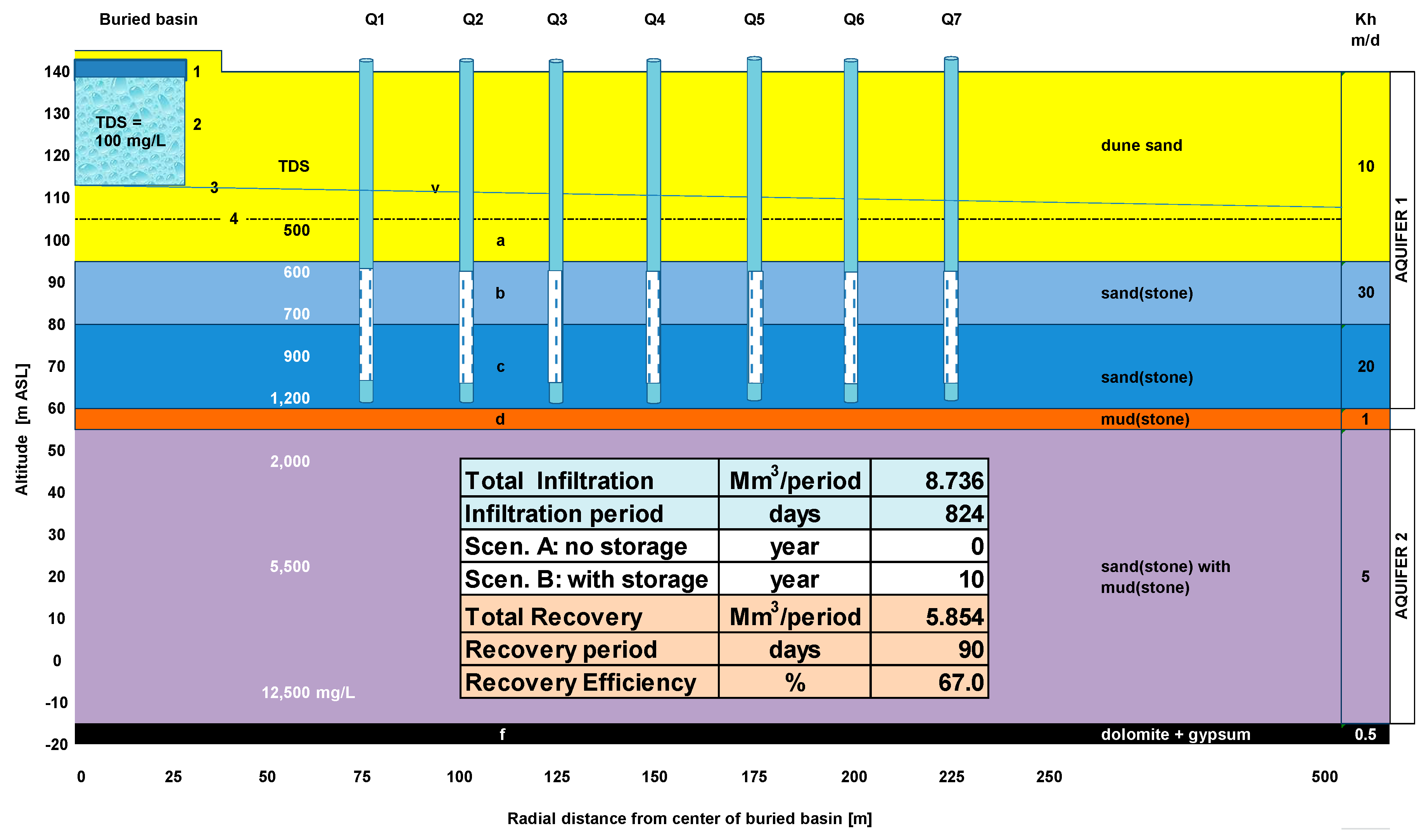
In EL, the whole ASR system was schematized by one representative recharge basin (the average of basins A–C), 5 aquifer layers (of which the upper layers a, b and c are most important) and 7 flowlines within each aquifer layer departing from the basin towards one recovery well in each of the 7 well rings at 75–225 m radius (Figure 5).

The expansion of the DSW bubble in each aquifer layer and the travel times along each flowline were calculated by assuming first vertical flow down to each aquifer layer and then horizontal radial flow, so that:

$$t_N=\frac{n_N \pi r^{2}T}{Q_{IN} K_{h,N}}+t_V$$

(4)

where: t_N = 50% break-through time (t₅₀) in layer N [d]; n_N = porosity of layer N [-]; r = radial distance from the basin center [m]; T = transmissivity of the aquifer [m²/d]; Q_IN = mean infiltration rate [m³/d]; K_h,N = horizontal hydraulic conductivity of layer N [m/d]; and t_V = vertical travel time [d] as determined by a 3D hydrological model [8].

This simplification creates some distortion during the first 30 d, but these are of minor importance on the long run of 824 d of infiltration. With Equation (4), the travel time was calculated from recharge basin to its 7 surrounding rings of recovery wells at the distances specified in Figure 6. It is deduced that in theory all wells, also those in the outermost ring will pump DSW after 824 d of infiltration. In layers D and E, probably little DSW will be present.

During 10 years of storage, the infiltrated DSW bubble is predicted to move laterally down the regional hydraulic gradient, with the following velocity (v_B,N), assuming an equal gradient in each layer:

$$v_{B,N}=\frac{K_{h,N} \Delta H}{n_N \Delta X}$$

(5)

where ΔH/ΔX = mean regional hydraulic gradient in the aquifer at well fields A, B and C during storage phase [m/m].

Vertical bubble drift by buoyancy has been ignored in accordance with FEFLOW model predictions [9]. The water quality evolution during injection phase was calculated for each flowline where it crossed its destination well (node point), and also for the “fictive”, mixed sample taken from all 35 node points, in proportion to: (i) the preset pumping regime (the inner wells pumping more than the outer wells); and (ii) the transmissivity of each main contributing aquifer layer (a–c). This mixed sample thus represents the output from the whole well field, when pumping out a negligible amount of water without disturbing the continuous DSW bubble expansion.

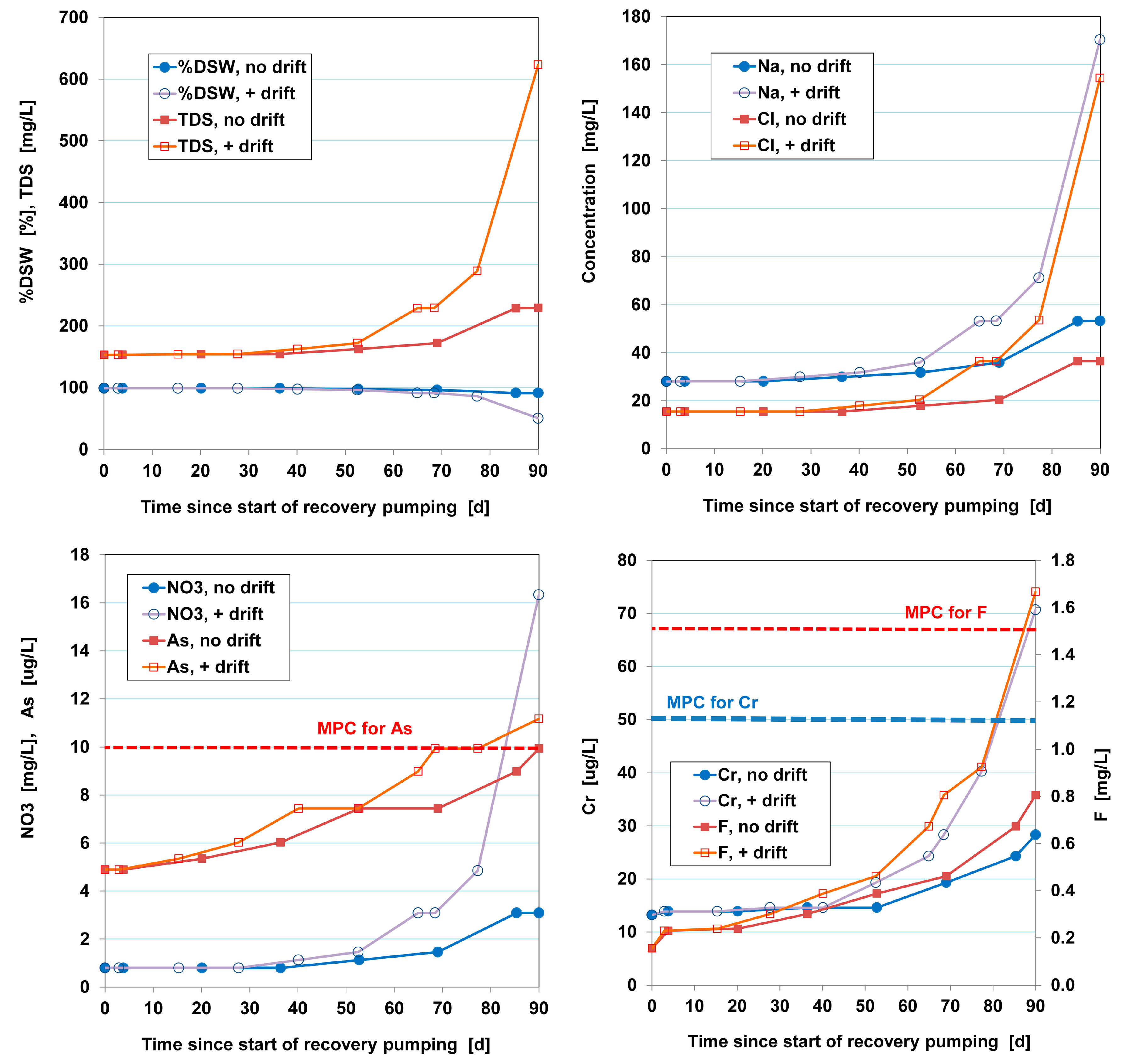
EL in forward mode assumes the following: (1) input quality (DSW) is constant; (2) retardation factors, leach factors and the (semi)permanent concentration changes are derived from observations during the pilot; (3) redox reactions are absent as observed in the pilot; (4) reactive minerals such as calcite, dolomite and silicates are not depleted; and (5) reaction kinetics do not play an important role.

The recovery phase was modeled by moving backward in the time series that displays the quality evolution of this “imaginary”, mixed (averaged) water sample. Contrary to the infiltration phase, this “imaginary”, mixed sample now becomes the true output of the well field during recovery phase, showing after some time an increasing instead of decreasing contribution of native groundwater. This is in harmony with theory and the predictions by [9,11].

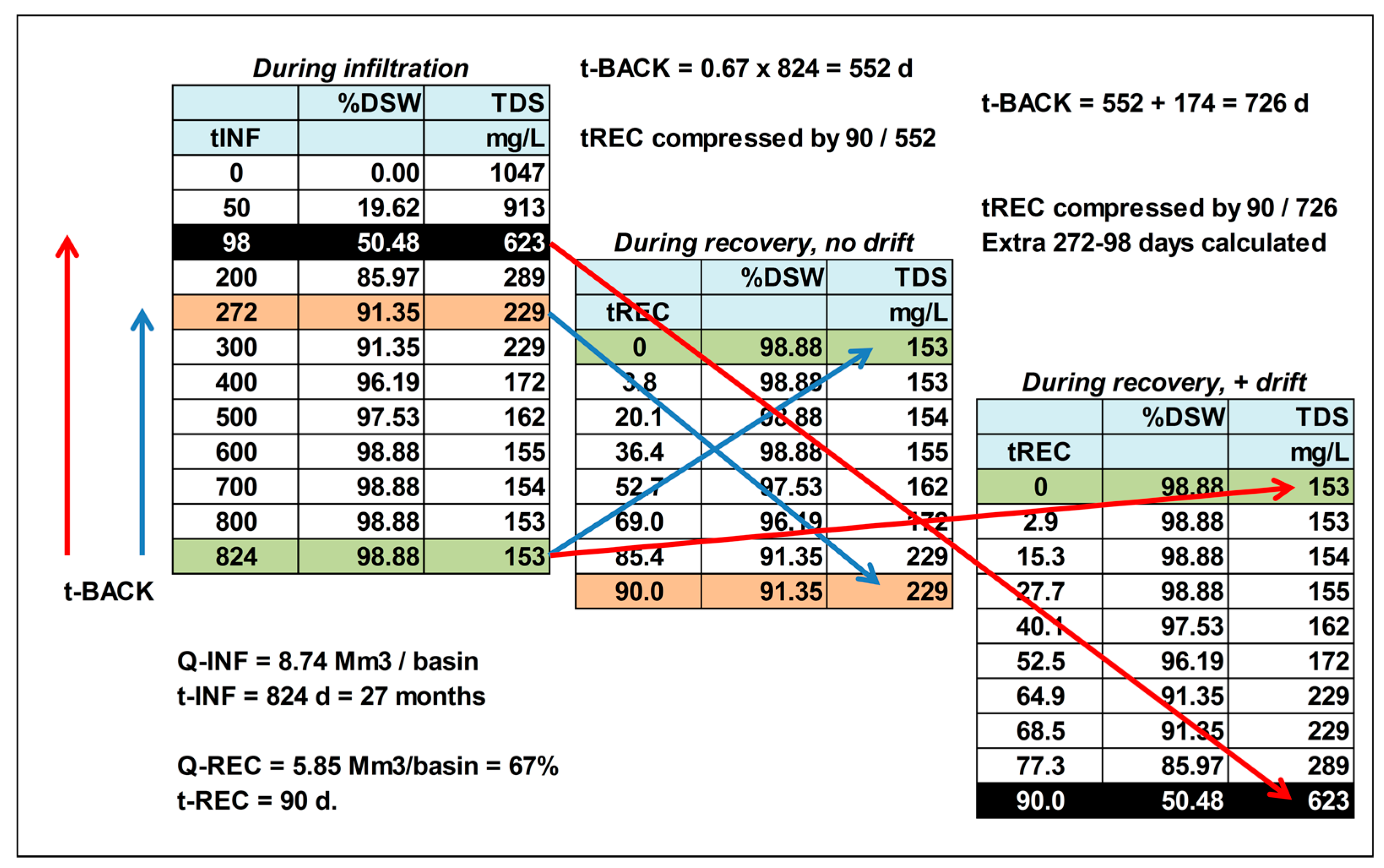
As during the 90 d of recovery 67% of the infiltrated water volume will be pumped out, the way back in the expansion time series needs to be as long as 0.67 × 824 = 552 d (= Δt_BACK-1). This way, water quality at the start of recovery, without storage phase, will be the water that flushed each of the 7 well rings prior to pumping (on day 824), and this water only needs to be mixed in proportion to the pumping rates of each well ring (Figure 6). At the end of pumping (after 90 d) we obtain about the same water as predicted to surround the wells on day 824 − 552 = 272. Water compositions in between can be calculated by just following the predicted water quality from 824 to 272 d back in time. In order to plot this water quality evolution during 90 d of recovery, the expanded time scale (from 90 to 552 d) needs to be compressed back again to 90 d, by multiplying it with 90/552, and to mirror it from backward into forward mode (Figure 7).

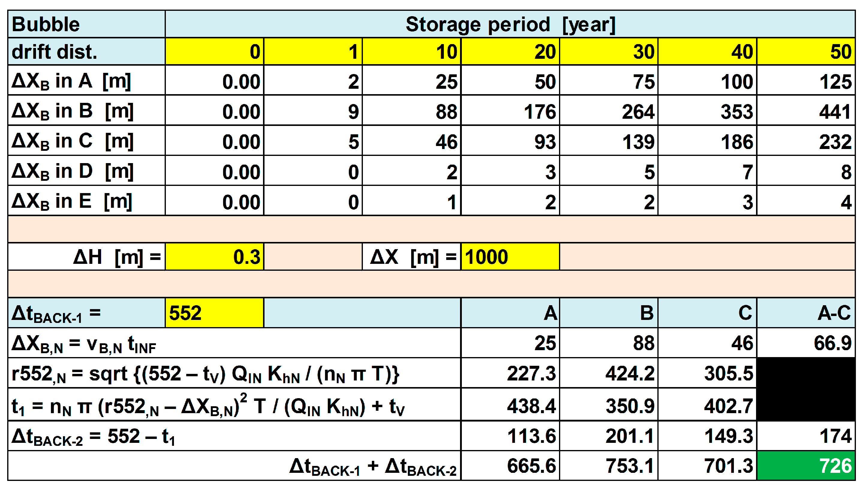
In the case of a 10-year storage phase, lateral bubble drift can be taken into account by first extending the backward period of 552 d (Δt_BACK-1) with the period (=Δt_BACK-2) that would be needed to get the retrograded bubble face back on its position at 552 d without bubble drift, and then resetting the time scale to 90 d by multiplying it with 90/(552 + Δt_BACK-2), and mirror it from backward into forward mode (Figure 7 and Figure 8).

The calculation of Δt_BACK-2 is then as indicated in the realistic example elaborated in Figure 8. In order to simplify the calculations, the weighted average value of Δt_BACK-2 is taken, being 174 d in the example of Figure 6. Addition of Δt_BACK-2 = 552 yields a total set-back time of 726 d. This means that the quality of the water recovered after 90 d of pumping, is to be looked up in the quality output list on day 824 − 726 = 98, in case of bubble drift during 10 years of storage.

How this example with resulting time shifts works out in the %DSW and TDS concentration of the water recovered, is shown in Figure 7. The underlying calculations were performed in EL, and match the predictions by [9] quite well.

EL in backward mode assumes that: (a) the forward evolution is reversed at 6 times higher speed; (b) the 6 times higher recovery rate does not provoke serious upconings (as shown by 3D modeling results [9]; and (c) during storage and recovery no further reactions with the aquifer are taking place.

Fluxes in the different aquifer layers, from the recharge basin towards the recovery wells and beyond them, were set equal to their contribution to the aquifer’s transmissivity.

Model calibration was done on: (1) available data from the pilot study in 2003–2004 when DSW was infiltrated via a recharge basin; and (2) groundwater quality as observed in the same pilot area in August 2014, after about 6 years of storage in the local aquifer system (since a second recharge run in 2008).

3. Results of Hydrogeological, Geochemical and Hydrochemical Stratification Analysis

3.1. Hydrogeology

The hydrogeological schematization is presented in Figure 5. It shows an upper aquifer with transmissivity 768 m²/d, formed by layers a–c, which consist of reddish to yellowish brown, eolian sand(stone) of Quaternary age. It is unsaturated in its upper 30 m, and consists there mostly of uncemented or weakly cemented sand. From the groundwater table downwards to the aquifer base at 62 m ASL, an alternation is observed of semi-consolidated and weakly to moderately cemented sands and sandstone.

Aquitard 1 and Aquifer 2, between 62 m ASL and 14 m BSL, likely correspond to the Pleistocene Medinat Zayed formation, consisting of mainly eolian and some fluvial and lacustrine deposits [11]. It is composed of yellowish brown to red brown to gray calcarenaceous sandstone with intercalations of siltstone, mudstone, marl and thin sand lenses.

Aquitard 2, at the base of the considered aquifer complex, is composed of a Neogene formation [11], consisting of light gray to white calcarenite, limestone and dolomite with interbeds of white to pinkish gypsum, marl, and chalk.

3.2. Geochemistry

The mean geochemical stratification (

Table 1. Simplified geochemical stratification as derived from [23]. BOM = bulk organic material; CEC = Cation Exchange Capacity.

Layer No.	Top m ASL	Base m ASL	Quartz	Calcite	Dolomite	Feldspar	Clay Min.	Others	BOM	Gypsum	Apatite mg/kg	pH-H2O	CEC meq/kg
			% d.w.
A	140	96	67.8	10.3	4.0	10.6	4.0	1.3	1.9	<0.1	0	8.10	61.3
B	96	80	83.0	2.9	2.3	9.2	1.5	1.7	0.5	<0.1	123	8.12	19.0
C	80	62	71.8	6.2	2.5	10.6	1.6	1.7	0.9	<0.1	154	8.18	28.1
D	62	56	47.0	19.9	18.3	6.0	18.2	1.3	0.5	<0.1	956	8.00	136.7
E	56	−14	54.6	13.9	12.8	5.4	17.1	1.6	1.6	0.1	83	7.89	146.6
F	−14	<−40	0.9	16.6	80.1	0.0	0.2	6.9	1.8	2.7	0	7.90	31.5

) follows more or less the hydrogeological subdivision (Figure 5). The interpreted data reveal the presence of the following reactive phases in the aquifer system, with their main potential interaction with water within brackets: Bulk Organic Material (denitrification, sorption), clay minerals (sorption), iron (hydr)oxide coatings of sand grains (source of Fe and oxyanions like chromate, vanadate and arsenate), calcite and dolomite (or dolomitic limestone; source of Ca, Mg, Sr and HCO₃), feldspars (source of Na, Ca and SiO₂), gypsum (source of Ca, Sr and SO₄), pyroxene (source of oxyanions like chromate, vanadate and arsenate), and (fluoro)apatite (source of Ca, PO₄ and F). Gypsum and dolomite were concentrated in aquitard 2 (at the base), feldspar and iron (hydr)oxides in aquifer 1 (the top).

The eolian sand is typically coated with iron (hydr)oxide, and more or less cemented mainly by calcite. The iron hydroxide coatings are considered to be the main (but genetically the secondary) source of oxyanions like chromate [Cr(VI)], vanadate, molybdate, selenate, arsenate and phosphate. These negatively charged ions are (chemi)sorbed to these positively charged coatings, and may desorb from it under specific conditions.

Another mineral frequently mentioned by [12], in concentrations of ≤1%, is pyroxene. Pyroxenes are of particular interest due to their potential contribution to Cr. Their composition is as follows: XY(Si,Al)₂O₆ with X representing Ca, Na, Fe(II), Mg and more rarely Zn, Mn and lithium, and Y representing Cr, Al, Fe(III), Mg, Mn, Sc, Ti and V. There is indeed a good positive correlation between Cr, Al, Fe, Ni, Ti, V and Zn [23], indicating that pyroxenes could be a significant primary source of Cr. No mention was made of the occurrence of olivine, another mineral typical of ophiolites, which [28] suspect as being the primary source of Cr in Abu Dhabi’s groundwater. This mineral has a high weathering thus low resistance potential, and has possibly therefore not been found.

3.3. Chemistry of Native Groundwater

The strong vertical zonation of water qualities in the aquifer system is mainly linked to a rising salinity (TDS) with depth (Figure 5). The latter is dictated by the presence of shallow “fresh” groundwater on top of deep seated brackish to saline paleowater [11]. The “fresh” groundwater, with a low Cl/Br ratio and high stable isotope content, is considered to be derived from local precipitation during relatively warm and humid climatic conditions with high evaporation losses, without significant contributions from evaporite dissolution [11,29]. The brackish to saline paleowater, with a high Cl/Br ratio and low stable isotope content, is considered to be derived from rainwater that dissolved evaporitic rock during relatively cold climatic conditions with less evaporation losses [11,29].

The following parameters follow the salinity (TDS) increase with depth: EC, Cl, SO₄, NO₃, Na, Fe, Mn, Al, B, Br, Cr, Cr(VI), Mo, Ni, Sr and Cl/Br ratio, whereas HCO₃, Ba and Ca/Mg ratio decline with depth (

Table 2. Simplified chemical stratification of the native groundwater, averaged over both pilot and ABC plant areas. Aquifer 1 = layers a–c; Aquitard 1 = layer d; Aquifer 2 = layer e. Abu Dhabi drinking water standards according to [13], WHO guidelines according to [31], both with red numbers for parameters considered at risk during ASR recovery. All samples showed: Ag < 1, Be < 0.1, Pb < 5 μg/L.

Sample	Layer # Figure 5		a	b	c	d	e-Top	e-Base	Abu Dh. Drinking w. Standard	WHO 2011 Guidelines
	Depth	m ASL	140	96	80	62	56	35
			96	80	62	56	35	−14
General	O2	mg/L	0.9	2.0	2.2	2.3	2.5	0.0	>2
	Temp.	°C	34.0	34.1	34.5	34.5	34.8	31.0
	EC 20 °C	μS/cm	969	1180	2132	4095	5650	17,647	1600
	TDS	mg/L	682	803	1545	2957	4042	13,288	1000
	pH	lab	7.83	8.25	8.09	7.92	7.94	7.40	7−9.2
Main constituents	Cl	mg/L	187	233	396	978	1506	5500	250
	SO4		147	152	397	702	844	3137	250
	HCO3		81	101	154	148	144	39	>60
	NO3		25.0	30.8	37.4	41.7	42.6	96.0	50	50
	PO4		0.022	0.034	0.029	0.028	0.030	0.015	2.2
	F		1.29	1.50	3.61	3.29	2.39	0.75	1.5	1.5
	Na		141	209	466	877	1204	3238	150
	K		12.9	11.7	11.5	15.8	18.5	83.7	12
	Ca		41.7	26.2	29.8	107.3	174.8	821.0	80
	Mg		10.7	7.0	11.2	41.1	67.0	340.0	30
	Fe		0.005	0.023	0.022	0.012	0.019	<0.44	0.2
	Mn		0.004	0.008	0.008	0.020	0.037	0.030	0.4
	NH4		0.015	0.025	0.019	0.015	0.015	0.035	0.5
	SiO2		26.2	23.1	28.4	27.8	23.6	14.3
	DOC		0.3	1.0	0.6	1.5	2.6	5.3	1
Trace elements	Al	μg/L	3	19	19	19	23	<290	200
	As		2.1	11.4	9.6	6.0	4.7	<10	10	10
	B		605	774	1113	1330	1421	1340	2400	2400
	Ba		40	38	31	33	36	23	700	700
	Br		579	668	788	762	767	301
	Cd		0.08	0.05	0.05	0.06	0.08	<10	3	3
	Co		0.06	0.08	0.07	0.44	0.82
	Cr-tot		52	87	115	129	123	<286	50	50
	Cr(VI)		48	85	108	119	117
	Cu		0.3	0.7	0.9	0.3	0.3	<1	1000	2000
	Hg		0.02	0.23	0.13	0.02	0.04		6	6
	Mo		6	11	39	47	39	<10
	Ni		0.5	2.5	1.6	1.0	1.6		70	70
	Sb		<1	2.2	1.2	<1	<1		20	20
	Se		3.2	3.2	3.3	4.1	5.2	17.0	40	40
	Sr		3485	2846	7381	8486	6573	1700
	Ti		<0.5	<0.5	<0.5	0.6	0.7
	U		0.6	0.7	3.0	3.1	3.1			30
	V		29	77	95	71	49	<10
	Zn		3	16	7	2	2	<50	5000
Ratio’s	Cl/Br	mg/L-basis	323	348	503	1284	1963	18297
	Ca/Sr		12.0	9.2	4.0	12.6	26.6	482.9
	Ca/Mg		3.9	3.8	2.7	2.6	2.6	2.4
Mineral Sat.	Barite	Saturation Index	−0.12	−0.13	−0.14	−0.16	−0.20	−0.50
	Calcite		−0.06	0.15	0.13	0.10	0.13	−0.15
	Dolomite		−0.26	0.18	0.30	0.29	0.39	−0.15
	Fluorite		−0.82	−0.95	−0.29	−0.37	−0.68	−0.82
	Gypsum		−1.72	−1.96	−1.70	−1.42	−1.43	−0.02
	TIC	mmol/L	1.38	1.71	2.59	2.51	2.43	0.68

). All groundwater is (sub)oxic (containing little O₂ and much NO₃), more or less in equilibrium with calcite and dolomite (as expected on the basis of geochemistry), slightly undersaturated with respect to barite, and (strongly) undersaturated with respect to fluorite and gypsum (base of layer e excluded where near equilibrium with gypsum).

The current mean-annual rainfall of 40–60 mm/year [30] would be sufficient to sustain natural recharge by local precipitation at a rate of ~7.6 [11] or 11 mm/year [8]. Tritium data on samples taken close to the groundwater table, stable isotope data, fluoro-chlorinated hydrocarbons and reaction patterns of the groundwater table to recharge events confirm that recharge of groundwater is actually taking place [8].

Between well fields A, B and C some differences exist [23]. Well field B is the most saline at all depth levels. Well field C is the least saline and most homogeneous of all. Well field A forms an intermediate, and is therefore taken as a representative for the whole plant.

4. Results of Sampling Campaign in August 2014

The sampling campaign of 3–7 August 7 2014 revealed [23] that there was only limited bias in the 2003–2013 hydrochemical data set of well fields A, B and C, and that practically all (>95%) of dissolved Cr consists indeed of Cr(VI).

The following bias was deduced for the large data set 2003–2013: O₂ concentrations for all monitoring wells were too high due to oxygenation, and suspended fines raised the concentrations of PO₄, Fe, Mn, NH₄, Al, and possibly also Zn in many samples. In addition, the minimum detection limits (MDLs) could be lowered for Cd, Hg, Ni, and Sb. All hydrochemical data presented here have been corrected for the demonstrated bias, where possible.

5. Results of Pilot

The available monitoring data at the pilot in 2003–2004 and 2014 (some of which are in

Table 3. Overview of water quality at the pilot basin recharge scheme in 2003–2004 and in August 2014. The samples taken in 2014 refer to a second recharge trial in 2008 at the same pilot plant, and therefore represent DSW after six years of aquifer storage. DSW infiltrated in 2008 (not shown here) deviates only slightly from DSW sampled in 2014.

Loc		Unit	First Pilot 2003-4						Second Pilot 2008 (2014)
			RB-01	DSW	RB-01	RB-02	OB-01A	OB-07B	DSW	OB-01A	OB-07B
			Ambient	Input	Recovery Wells		Obs. Wells		Input	Obs. Wells
Space & time	Top screen	m ASL	93	121	93	91	104	100	121	104	100
	Base screen	m ASL	75	121	75	73	95	91	121	95	91
	Radial distance	m	83	0.0	83	30	44	90	0	44	90
	t50	d		0.0			11	50	0	11	50
	PVs	-	0.0	0.0	>3	>10	6.3	1.4	0.0	50.0	10.0
	Digital date	year	2003.70	2004.21	2004.35	2004.57	2003.94	2003.94	2014.59	2014.60	2014.60
Main composition	O2	mg/L	4.9	7.2			8.0		7.2	6.8	7.2
	EC 20 °C, lab	μS/cm	1313	397	487	432	413	512	123	134	142
	Temperature	°C	31.0	35.0	31.0	31.0	31.0	31.0	35.0	36.4	35.8
	pH-Lab	-	8.94	7.90	9.11	7.69	8.57	8.50	8.11	8.43	8.90
	Na	mg/L	266.0	45.7	107.0	57.2	46.3	104.0	4.1	7.4	25.9
	K	mg/L	6.1	1.6	2.7	8.1	10.4	7.8	<0.1	2.9	5.7
	Ca	mg/L	7.3	22.3	1.8	21.0	17.3	8.4	20.2	12.2	4.6
	Mg	mg/L	2.5	5.3	0.5	3.9	6.2	4.9	0.4	5.0	1.7
	Fe	mg/L	0.130	0.255	0.050	0.150	0.080	0.683	0.012	0.005	0.005
	Mn	mg/L	0.040	0.008	0.050	<0.01	0.020	0.008	0.003	0.003	0.003
	NH4	mg NH4/L	<0.1	<0.1	<0.1	<0.1	<0.1		<0.03	<0.03	<0.03
	SiO2	mg SiO2/L	27.3	2.1	24.0	24.0	18.2	4.6	<1	15.2	20.0
	Cl	mg/L	216.0	80.8	80.3	78.0	83.1	89.5	5.0	10.0	11.0
	SO4	mg/L	162.0	11.7	10.7	10.8	13.4	22.0	1.0	<2	2.0
	HCO3	mg/L	152	60	123	104	62	139	66	66	59
	TIC	mmol/L	2.64	1.01	2.16	1.78	1.04	2.33	1.11	1.11	1.01
	NO3	mg NO3/L	23.5	<0.5	0.0	0.0	<0.5	<0.5	<1	<1	<1
	NO2	mg NO2/L	0.01	<0.01			<0.01	0.004	<0.01	<0.01	<0.01
	PO4-total	mg PO4/L							0.21	0.06	0.02
	PO4-ortho	mg PO4/L	0.021	0.062			0.021	0.358	0.060	<0.03	<0.03
	F	mg/L	2.10	0.05	0.20	0.10	0.10	3.51	<0.05	0.06	0.26
	DOC	mg/L						8.4	<0.5	<0.5	<0.5
Trace elements	Al	μg/L	180	248	510	200	80	535	51	13	13
	As	μg/L	11.0	0.0			<3		<0.5	2.2	8.4
	B	μg/L	850	29	58	52	52		17	56	55
	Ba	μg/L	13	5	30	6	16	20	2	12	3
	Br	μg/L	570	20	301	301	140			161	186
	Cr	μg/L	95.0	2.5	17.0	15.0	13.0		<0.5	12.9	7.4
	Cu	μg/L	5.0	20.3	2.0	4.0	<2	<2	16.4	<0.5	<0.5
	Mo	μg/L	10.0	<3	<3	<3	<3	<3	<1	<1	<1
	Ni	μg/L	3.0	9.5	<3	<3	<3	<3	4.3	<1	<1
	Se	μg/L	<2	<2	3.0	3.0	<2		<0.5	<0.5	<0.5
	Sr	μg/L	1200	50	200	1600	1300	278	16	1000	274
	V	μg/L	66	1.5	140	36	17		<0.5	12	64
	Zn	μg/L	10	81	59	98	4	5	3	<2	<2
Mineral saturation	SI-B	Barite	−0.5	−1.8	−1.0	−1.7	−1.2	−0.9	−2.6	−2.4	−2.7
	SI-C	Calcite	0.5	−0.2	0.1	−0.3	0.3	0.2	0.0	0.2	0.0
	Si-D	Dolomite	0.9	−0.6	0.0	−0.9	0.5	0.6	−1.2	0.4	0.0
	SI-G	Gypsum	−2.4	−2.9	−4.0	−2.9	−2.9	−3.1	−3.2	−4.1	−4.2
	SI-B	Barite	−0.5	−1.8	−1.0	−1.7	−1.2	−0.9	−2.6	−2.4	−2.7
	SI-F	Fluorite	−1.1	−3.7	−3.6	−3.1	−3.2	−0.5	−4.3	−3.8	−2.9

) reveal among others the following quality changes of DSW in the aquifer:

• There are hardly any changes of O₂, Cl, SO₄, HCO₃, TIC, NO₃ and NH₄, even after six years of storage. This indicates that redox reactions were practically nonexistent, and carbonates (calcite and dolomite) hardly dissolved or precipitated.
• A small TDS increase (20–30 mg/L) by dissolution of mainly SiO₂, K and possibly Mg. Carbonate dissolution was noticed only where a very strong Ca/Na exchange was taking place (see next point).
• Ca/Na exchange in which Ca concentrations declined and Na increased was observed. This was especially important for samples close to the DSW intrusion front and typical for fresh water intrusion.
• Mobilization of the trace elements As, B, Ba, F, Cr, Sr and V from the aquifer, through desorption and/or mineral dissolution was observed. The strongest and most persistent increase is noticed for Sr, which does not exactly match Ca behavior, so that another mineral could be the source. Of the trace elements mentioned, Ba shows the smallest mobilization, whereas As, F and Cr show a significant leaching by DSW, which is also important from a drinking water quality perspective.
• Immobilization of PO₄, Al, Cu, Fe and Ni during aquifer passage was mainly by sorption of PO₄, Cu and Ni, and filtration of suspended colloidal particles of Al and Fe.
• Calculated mineral saturation indices show that the infiltrated water is more or less in equilibrium with calcite and dolomite as expected. The values for gypsum, barite and fluorite indicate a strong undersaturation.

These changes were subsequently plotted against dimensionless time parameter PV (Equation (1)), as shown for a selection of constituents in Figure 9. The resulting patterns were translated into leaching and retardation factors and semi-permanent concentration changes (

Table 4. Interpretation of water quality observations at the pilot, in terms of retardation factor (R), Leach factor (L) and (semi)permanent concentration change after break-through (ΔC).

Parameter	L	R	ΔC [mg/L]			Parameter	L	R	ΔC [ug/L]
			2003-4	2014					2003-4	2014
Na	1.5–2	--	3	3.5		F	1.5–2	--	0.2	0.04
K	20	--	3	3		Al	1.5	--	−130	−39
Ca	--	3.5	0	−8		As	3	--	1	2
Mg	--	3	3.3	4.5		B	2	--	10	30
Fe	2	--	0	0		Ba	--	--	10	10
SiO2	2–4	--	0.6	14.5		Cr	1.5–2	--	10	13
Cl	1	--	0	0		Mo	1.5	--	0	0
SO4	1	--	0	0		Ni	1.5	--	-8	−4
HCO3	1	--	0	0		Sr	--	3.5	1600	984
NO3	1	--	0	0		V	5	--	10	11
PO4-O	--	--	−0.04	−0.05		Zn	--	--	−60	−1.5

). These observations assisted in fine-tuning the EL model, which is partly based on both calculated and observed values of L, R and DC.

The plots in Figure 9 show the observed concentration trends for selected constituents as function of the dimensionless time parameter “pore volume” (PV). The following classification of elements with similar behavior can be made on the basis of their concentration/PV-plot.

• Ca, Mg and Sr (Ca and Mg shown in Figure 9) concentrations start low and with increasing PVs rise to an asymptotic value. All 2014 data plot below those of 2003–2004, which is partly explained by the lower DSW input in 2008. Only Ca and Mg show an initial concentration below DSW input, which is probably linked to Na exchange, with Ca developing an asymptotic value at or below DSW input. Contrary, Mg and Sr approach an asymptotic value little (Mg) or far (Sr) above DSW input. Obviously, Mg and even more so Sr are dissolved from the aquifer, and Ca is not. Sources of Mg and Sr could be dolomite and/or silicate minerals.
• SiO₂, K and V concentrations (SiO₂ and K shown in Figure 9) decline in an exponential way, but relatively slowly compared to the next group, and the low concentration asymptote is also relatively high and in most cases far above DSW input. This suggests that these elements are initially desorbed and that later on they could be dissolving from the aquifer, possibly from quartz (SiO₂), K-feldspar (K and SiO₂) or for instance pyroxenes (SiO₂ and V). A long storage time yields much higher concentrations for SiO₂, pointing at slow dissolution kinetics. Vanadium is likely present as VO₄³⁻, which could desorb from iron (hydr)oxide coatings.
• Na, As, B, Cr, F and Mo (Na and Cr shown in Figure 9) concentrations also decline in an exponential way, but much more rapidly than the previous group. The low concentration asymptote is relatively high and in any case significantly above DSW input, especially for As, B and Cr. The asymptote approaches DSW input better for Na, F and Mo. This suggests that all these elements are very rapidly desorbed and that later on especially As, B and Cr could be steadily dissolving from the aquifer matrix. Except for Na and B (as H₃BO₃), this group is composed of anions, As as AsO₄³⁻, Cr as CrO₄²⁻, F as F⁻ and Mo as MoO₄²⁻. The source mineral of chromate and vanadate could be pyroxenes [23].
• Al, Fe and Ni concentrations (Al shown in Figure 9) decline in an exponential way, approximately as rapidly as the previous group. Their concentration seems to be dictated by colloidal particles that become initially mobilized. On the one hand, lack of filtration may have contributed to this. On the other hand, it is well known [32], that clay minerals in aquifers tend to be mobilized by deflocculation when the sodium adsorption ratio (SAR) of the infiltration water and of the native groundwater is high, their salinity low, the clay mineral content high, and the dominant type of clay minerals unfavorable (smectite > illite > kaolinite). The SAR value of the native groundwater seems to be more important than the one of the infiltration water. With SAR values of ~20, the risk of mechanical clogging of the aquifer when the particles strand in the pore necks is relatively high. This risk is estimated higher in aquifer layer C than in A and B because SAR of native groundwater is higher and permeability is lower.

In Table 4, the estimated retardation (R) or leach factors (L) as derived from the PV-plots (Figure 9) are listed, together with the estimated (semi)permanent concentration increase (DC).

It can be concluded that those parameters that could cause problems with drinking water standards (Table 2), such as EC, TDS, Na, Cl, SO₄, F, As and Cr, are swiftly leached out from the aquifer, namely most of them within 1–3 PVs. The leach factor for Cr corresponds well with the chromate retardation factor as observed in a column dosage experiment [33], and with observations elsewhere [34,35].

The (semi)permanent concentration increases can, in general, be attributed to mineral dissolution or prolonged desorption from low permeability but high concentration pockets within the aquifer. The significant Ca decrease and Mg increase during the six-year storage period could point at dedolomitization, in which possibly also Sr²⁺ is involved:

$$\left(Y+Z\right)C{a}^{2+}+C{a}_{X}M{g}_{Y}S{r}_{Z}C{O}_3\leftrightarrow CaC{O}_3+Y M{g}^{2+}+Z S{r}^{2+}$$

(6)

where X + Y + Z = 1, possibly with Mg = 0.38 and Sr = 0.02.

The relatively strong increase for SiO₂ during the six-year storage period could at least partly be explained by quartz dissolution at the relatively high water temperatures (35 °C). The following relation by [36] can be used to predict quartz solubility at temperatures 0–200 °C, yielding 14.3 mg/L at 35 °C:

$$Si{O}_2={10}^{4.83-\frac{1132}{temp+273.15}}$$

(7)

6. Results of Predicting the Quality of Recovered Water

6.1. Model Settings

The SWSR ASR system was modeled for just one of three recharge basins, assuming this to be representative for all three basins. The applied hydrogeological and geochemical stratification of the aquifer system into five layers follows the information given in Section 3. The low TDS DSW was selected as constant input to the recharge basin. Its quality is shown in Table 3.

The travel times to all recovery wells (condensed into one well per ring) and flux contributions from each aquifer layer to the well discharge, were calculated as indicated in Section 2.7. The combination of travel times leads to the so-called response curve of the whole well field. This is defined as the cumulative frequency distribution of underground travel times from the recharge basin to the wells during infiltration. The resulting response curve is shown in Figure 10.

Water quality changes in the recharge basin were completely ignored, because of exclosure from both sunlight and direct atmospheric contact, the high quality of DSW and the expected ultralow concentration of suspended solids. The formation of bottom muds in the basin was excluded. The complete lack of redox reactions necessitated the setting of the reactivity of bulk organic material at zero.

6.2. Quality Evolution during Nonstop Infiltration

If the infiltration via one of the recharge basins of the SWSR facility would last for 100 years without interruption, and the recovery wells would periodically pump out a water sample during this period varying between 0.1 and 100 years, then the abstracted water quality would be as predicted in

Table 5. Overview of water quality in the SWSR ASR scheme, showing input DSW (Desalinated Seawater), mean native groundwater (when sampled by all wells) and groundwater as if it were periodically sampled after 0.1 to 100 years during nonstop DSW infiltration.

Sample	Parameter	Unit	Native	RECOVERED WATER ‘SAMPLED’ AFTER						Input	Abu Dh. Drink. w. Standard	WHO Guide-Lines
			Measured	0.1	0.27	0.74	2.26	10	100	DSW
			at ABC	Year	Year	Year	Year	Year	Year	2014
General	EC 20 °C	μS/cm	1411	1304	829	295	199	184	170	123	1600
	Temp.	°C	34.2	34.2	34.4	34.8	35.0	35.0	35.0	35.0
	pH		8.13	8.13	8.20	8.35	8.44	8.44	8.45	8.10	7–9.2
	O2	mg/L	1.9	2.5	4.5	6.7	7.1	7.1	7.1	7.2	>2
	CH4	mg/L	0.00	0.00	0.00	0.00	0.00	0.00	0.00	0.00
	DOC	mg/L	0.8	0.8	0.6	0.4	0.3	0.3	0.3	0.3	1
	SI-calcite		0.19	0.15	0.00	−0.30	−0.19	0.18	0.33	0.00
Main constituents	Cl	mg/L	287.0	261.6	154.5	36.5	15.4	11.5	7.8	5.0	250
	SO4	mg/L	235.0	217.8	130.7	28.0	8.3	5.9	3.6	1.0	250
	HCO3	mg/L	116	112	93	71	67	67	67	66	>60
	NO3	mg/L	32.3	29.0	16.3	3.1	0.8	0.7	0.6	0.3	50	50
	PO4	mg/L	0.03	0.03	0.03	0.03	0.05	0.16	0.21	0.21	2.2
	Na	mg/L	295.0	273.2	170.4	53.3	28.0	13.1	7.2	4.1	150
	K	mg/L	12.4	11.1	6.8	2.0	0.7	0.3	0.2	0.1	12
	Ca	mg/L	31.5	28.7	17.9	6.3	6.4	15.4	20.6	20.2	80
	Mg	mg/L	9.5	8.8	5.7	2.2	2.1	2.6	0.7	0.4	30
	NH4	mg/L	0.02	0.02	0.02	0.02	0.01	0.00	0.00	0.02	0.5
	Fe	mg/L	0.02	0.02	0.02	0.02	0.02	0.01	0.00	0.012	0.2
	Mn	mg/L	0.01	0.00	0.00	0.00	0.00	0.00	0.00	0.003	0.4
	SiO2	mg/L	25.2	25.2	25.2	25.2	23.0	14.4	14.4	0.5
Trace elements	As	μg/L	11.2	11.2	11.2	9.9	4.9	2.0	1.9	0.3	10	10
	B	μg/L	884	884	736	311	65	48	44	17	2400	2400
	Ba	μg/L	46	46	46	46	46	31	14	2	700	700
	Cr	μg/L	104.0	103.7	70.7	28.3	13.2	13.0	12.6	0.30	50	50
	Cu	μg/L	0.7	0.7	0.7	0.7	2.4	11.9	16.2	16.4	1000	2000
	F	μg/L	2190	2113	1667	895	173	101	92	30	1.5	1.5
	Ni	μg/L	2.0	2.0	2.0	2.0	2.2	3.4	4.3	4.3	70	70
	Sr	μg/L	4397	4397	4397	4397	4397	2889	228	16
	V	μg/L	87	87	83	54	16	11	11	0.3
	Zn	μg/L	12.0	11.6	11.6	11.6	11.6	5.4	3.0	3.0	5000

. This table also shows the quality of DSW prior to infiltration and of native groundwater as abstracted by all ABC recovery wells.

Many things can be concluded from this table, because the recovered water quality also covers those moments that are representative for the 90 d recovery with or without drift. That aspect follows in Section 6.3.

Here, it is concluded that continued flushing leads to an initially fast and then slow elution of native groundwater, a significant leaching of the trace elements As, B, Ba, Cr, F and Sr, and a slow breakthrough of Cu, Ni and Zn which show higher concentration levels in DSW than in native groundwater. For selected elements, the breakthrough or leaching curves have been plotted in Figure 11. The bulk of changes clearly happens during the first year when the native groundwater is displaced.

The predicted water quality after 0.27 year is also representative of water quality after 90 d recovery following 10 years of lateral drift after 824 d of DSW infiltration. The quality after 0.74 year is as the one after 0.27 year, but without lateral drift (thus, with direct recovery). The quality after 2.26 years is the water that is recovered on the first day after 824 d of DSW infiltration.

6.3. Quality Evolution during Recovery

The standard EL output list had to be elaborated, as indicated in Figure 7, in order to depict the water quality evolution during the 90 d of recovery (with or without 10 years standstill before). The result is shown for selected elements (Na, Cl, NO₃, As, Cr and F), TDS and the contribution of DSW in Figure 12, and for many more water quality parameters in Table 5.

It is concluded that TDS and the concentration of most dissolved constituents slowly rise, while the percentage of DSW slowly decreases during progressive recovery. The main reason of this worsening water quality is the admixing of native groundwater. Without a preceding 10-year storage phase and thus practically without bubble drift, recovered water quality complies with the UAE drinking water standards (Table 2), with only As approximating the maximum permissible concentration near the end.

Ten years of storage with bubble drift have a more negative impact on water quality, as expected. This becomes manifest only halfway during the 90 d recovery phase (Figure 12), and starts to become critical in between 80 and 90 d, especially regarding Na, As, Cr and F. These constituents are predicted to exceed the drinking water MPCs: Na 170 (MPC 150 mg/L), As 11.2 (MPC 10 ug/L), Cr 70.7 (MPC 50 ug/L) and F 1.67 (MPC 1.5 mg/L).

7. Discussion

The relatively simple modeling approach as presented in Section 2.7 and applied in Section 6, strongly relies on: (i) observations done during trials in the pilot area; and (ii) reversibility of the predicted water quality evolution during forward (infiltration) mode. This means that complications due to shorter or longer detention times in the aquifer (during storage and recovery) or due to processes like biofouling of the basin proximal zone should not occur.

Problematic deviations from our predictions could arise, when the relatively high recovery rate (six times higher than the infiltration rate) would provoke serious upconing of brackish to saline groundwater from Aquifer 2, or when pockets of lower permeability in aquifer 1 would deliver more of their interstitial, low quality groundwater. A more dedicated spatial model, in which density effects and reactive transport (e.g., [19]) are combined, is needed to assess the potential impact of these processes.

There are other important questions still to answer, probably necessitating column studies and prolonged field monitoring during operation. The first question is: Which mineral sources could be responsible for the remarkable, semipermanent background mobilization of especially Cr, V, As and Sr, and how can this mobilization be mitigated? The second is whether clay minerals will deflocculate upon flushing of the target aquifer, and thereby clog it. There are weak signs that this might have happened to a minor degree during the pilot. The risk of clay mobilization will be higher during the operational phase, because still lower TDS infiltration water (DSW) will be used, and the ABC area contains some higher salinity subareas than the pilot area.

8. Conclusions

In this paper, we present the peculiar characteristics of an eolian-fluvial, (sub)oxic, calcareous sand(stone) aquifer system in a desert environment, the unique water quality changes during an ASR pilot including a six-year storage phase, and a relatively simple modeling approach to rapidly predict water quality of the recovered water, which is to be distributed without treatment.

In the applied Easy-Leacher model, pilot observations on retardation, leaching and (semi)permanent concentration changes are combined with a strong schematization of the complex basin–ASR system, groundwater flow (including bubble drift) and hydrogeochemical processes.

The hydrogeochemical simplifications are justified by the low reactivity of the aquifer, which is explained by the very low solute content of desalinated seawater (DSW), the infiltration of (sub)oxic DSW into an already (sub)oxic aquifer (thus, preventing redox reactions), a rapid leaching and, at high pH (7.8–8.5), high mobility of the problematic trace elements Cr (>95% as CrO₄²⁻), B (as H₃BO₃), F, Mo (as MoO₄²⁻), and V (as VO₄³⁻).

The pilot observations and modeling results demonstrate that recovered water is most likely complying with Abu Dhabi’s drinking water standards in both studied ASR scenarios. Without preceding 10-year storage (and thus hardly any drift, but with replacement of native groundwater), recovered water quality is expected to comply with the drinking water standards after 824 d of infiltration, even beyond the 67% recovered in 90 d (up to ~85% recovery). The same conclusions also hold for the modeled scenario with 10-year storage (and thus significant bubble drift), however not for 90 but for 80 d. This means that the recovery efficiency will drop from ~85 to 60%. After 80 d (60% recovered), MPC exceedances are then expected for: Na (20 above 150 mg/L), As (1 above 10 μg/L), Cr (21 above 50 μg/L) and F (0.2 above 1.5 mg/L). The main reason for their exceedances is the admixing of native groundwater.

This prediction has contributed to the implementation of some adaptations to the current ASR scheme operational since May 2015. The injection rate was raised by 20%, and during storage 568 m³/d will be infiltrated continuously during any storage period. By adjusting pumping schemes based on real time monitoring, the recovery efficiency can probably be maintained at about 80%.

If drinking water standards would become more strict, as is currently discussed in the Netherlands regarding As (from 10 to 1 μg/L) and CrO₄²⁻ (from 50 to 0.3 μg/L; [37]), then Abu Dhabi’s drinking water standards will be exceeded in all modeled cases. This may be acceptable, however, during a short emergency situation after a calamity.

Potential risks of upconing of brackish/saline deep, native groundwater, aquifer clogging by clay mobilization and basin clogging were not addressed, and may necessitate further research.

References

1. Saif, O. The Future Outlook of Desalination in the Gulf: Challenges & Opportunities Faced by Qatar & the UAE. 2012. Available online: http://inweh.unu.edu/wp-content/uploads/2015/05/The-Future-Outlook-of-Desalination-in-the-Gulf1.pdf (accessed on 2 January 2017).
2. Al Shehhi, M.R.; Gherboudj, I.; Ghedira, H. An overview of historical harmful algae blooms outbreaks in the Arabian Seas. Mar. Pollut. Bull. 2014, 86, 314–324. [Google Scholar] [CrossRef] [PubMed]
3. Do Rosário Gomes, H.; Goes, J.L.; Matondkar, S.G.P.; Buskey, E.J.; Basu, S.; Parab, S.; Thoppil, P. Massive outbreaks of Noctiluca scintillans blooms in the Arabian Sea due to spread of hypoxia. Nat. Commun. 2014, 5. [Google Scholar] [CrossRef] [PubMed]
4. Missimer, T.M.; Sinha, S.; Ghaffour, N. Strategic Aquifer Storage and Recovery of Desalinated Water to Achieve Water Security in the GCC/MENA Region. Int. J. Environ. Sustain. 2012, 1, 87–99. Available online: https://www.sciencetarget.com/Journal/index.php/IJES/article/viewFile/93/26 (accessed on 2 January 2017). [Google Scholar] [CrossRef]
5. Hutchinson, C.B. Simulation of Aquifer Storage Recovery of Excess Desalinated Seawater; U.S. Geological Survey Open-File Report 98-410; USGS: Al Ain area, Abu Dhabi Emirate, 1998. Available online: https://pubs.usgs.gov/of/1998/0410/report.pdf (accessed on 2 January 2017).
6. Pyne, R.D.G.; Howard, J.B. Desalination/aquifer storage recovery (DASR): A cost effective combination for Corpus Christi, Texas. Desalination 2004, 165, 363–367. [Google Scholar] [CrossRef]
7. Dawoud, M.A.; Sallam, O.M. Sustainable Groundwater Resources Management in Arid Regions: Abu Dhabi Case Study; Environmental Agency Abu Dhabi Report; Environmental Agency Abu Dhabi: Abu Dhabi, United Arab Emirates, 2010.
8. German Technical Cooperation Agency. Combined Artificial Recharge and Utilisation of the Groundwater Resource in the Greater Liwa Area (Western Region of the Emirate of Abu Dhabi); Pilot Project Final Technical Report; Deutsche Gesellschaft für Technische Zusammenarbeit (GTZ) GmbH in Co-operation with Dornier Consulting (DCo) GmbH: Bonn, Germany, 2005. [Google Scholar]
9. German Technical Cooperation Agency. Detailed Design Groundwater Modelling Final Report; Consultancy Services for Artificial Recharge and Utilisation of the Groundwater Resource in the Liwa Area, Consultancy Contract No. G 4877; Deutsche Gesellschaft für Technische Zusammenarbeit (GTZ) GmbH in Co-operation with Dornier Consulting (DCo) GmbH: Bonn, Germany, 2009. [Google Scholar]
10. German Technical Cooperation Agency. Detailed Design Drilling, Construction and Testing of Recovery and Monitoring Wells Draft Report; Consultancy Services for Artificial Recharge and Utilisation of the Groundwater Resource in the Liwa Area, Consultancy Contract No. G 4877; Deutsche Gesellschaft für Technische Zusammenarbeit (GTZ) GmbH in Co-operation with Dornier Consulting (DCo) GmbH: Bonn, Germany, 2009; p. 56. [Google Scholar]
11. Earth Link & Advanced Resources Development. Hydrogeological Study and Numerical Groundwater Simulation; Construction Phase Strategic Water Storage and Recovery Project in Liwa Abu Dhabi—United Arab Emirates; Quarterly Report #6 Hydrogeological Structure and Groundwater Flow & Transport Model of the SWSR Region; Earth Link and Advanced Resources Development Sarl: Amaret Chalhoub, Lebanon, 2013. [Google Scholar]
12. Al Futtaim Exova LLC. Test Report of Core Samples; 4 Reports on Respectively Well No: MW 01C, MW11C, MW21 and MW42; Al Futtaim Exova LLC, Lab: Dubai, United Arab Emirates, 2011–2012. [Google Scholar]
13. Water Quality Regulations 2013-Final Draft Consultation; Regulation and Supervision Bureau Abu Dhabi: Abu Dhabi, United Arab Emirates, 2013.
14. Stuyfzand, P.J. Quality changes upon injection into anoxic aquifers in the Netherlands: Evaluation of 11 experiments. In Artificial Recharge of Groundwater, Proceedings of the 3rd International Symposium on Artificial Recharge, Amsterdam, The Netherlands, 21–25 September 1998; Peters, J.H., Ed.; Balkema: Amsterdam, The Netherlands, 1998; pp. 283–291. [Google Scholar]
15. Stuyfzand, P.J.; Timmer, H. Deep Well Injection at the Langerak and Nieuwegein sites in the Netherlands: Chemical Reactions and Their Modeling; Kiwa-SWE 99.006; KWR Watercycle Research Institute: Nieuwegein, The Netherlands, 1999; 44p. [Google Scholar]
16. Stuyfzand, P.J. Pyrite oxidation and side-reactions upon deep well injection. WRI-10. In Proceedings of the 10th International Symposium on Water Rock Interaction, Villasimius, Italy, 10–15 June 2001; Volume 2, pp. 1151–1154.
17. Prommer, H.; Stuyfzand, P.J. Identification of temperature-dependent water quality changes during a deep well injection experiment in a pyritic aquifer. Environ. Sci. Technol. 2005, 39, 2200–2209. [Google Scholar] [CrossRef] [PubMed]
18. Antoniou, E.A.; van Breukelen, B.M.; Putters, B.; Stuyfzand, P.J. Hydrogeochemical patterns, processes and mass transfers during aquifer storage & recovery (ASR) in an anoxic sandy aquifer. Appl. Geochem. 2012, 27, 2435–2452. [Google Scholar]
19. Zuurbier, K.G.; Hartog, N.; Stuyfzand, P.J. Reactive transport impacts on recovered freshwater quality during multiple partially penetrating wells (MPPW-)ASR in a brackish heterogeneous aquifer. Appl. Geochem. 2016, 71, 35–47. [Google Scholar] [CrossRef]
20. Pyne, R.D.G. Aquifer Storage Recovery—A Guide to Groundwater Recharge through Wells; ASR Systems LLC: Gainesville, FL, USA, 2005. [Google Scholar]
21. Price, R.E.; Pichler, T. Abundance and mineralogical association of arsenic in the Suwannee Limestone (Florida): Implications for arsenic release during water-rock interaction. Chem. Geol. 2006, 228, 44–56. [Google Scholar] [CrossRef]
22. Wallis, I.; Prommer, H.; Simmons, C.T.; Post, V.; Stuyfzand, P.J. Evaluation of Conceptual and Numerical Models for Arsenic Mobilization and Attenuation during Managed Aquifer Recharge. Environ. Sci. Technol. 2010, 44, 5035–5041. [Google Scholar] [CrossRef] [PubMed]
23. Stuyfzand, P.J.; Smidt, E.; Zuurbier, K.G. Baseline Hydrogeochemistry of the Strategic Water Storage and Recovery Project in Liwa, Abu Dhabi; KWR-Report KWR2014.073; KWR Watercycle Research Institute: Nieuwegein, The Netherlands, 2014. [Google Scholar]
24. Stuyfzand, P.J.; Hartog, N.; Smidt, E. Prediction of Recovered Water Quality of the Strategic ASR Project in Liwa, Abu Dhabi; KWR-Report KWR2015.003; KWR Watercycle Research Institute: Nieuwegein, The Netherlands, 2014. [Google Scholar]
25. Stuyfzand, P.J. Simple models for reactive transport of pollutants and main constituents during artificial recharge and bank filtration. In Artificial Recharge of Groundwater, Proceedings of the 3rd Internatioanl Symposium on Artificial Recharge, Amsterdam, The Netherlands, 21–25 September 1998; Peters, J.H., Ed.; Balkema: Amsterdam, The Netherlands, 1998; pp. 427–434. [Google Scholar]
26. Stuyfzand, P.J. Hydrogeochemcal (HGC 2.1), for Storage, Management, Control, Correction and Interpretation of Water Quality Data in Excel (R) Spread Sheet; KWR-Report BTO2012.244(s); Updated in 2016 December; KWR Watercycle Research Institute: Nieuwegein, The Netherlands, 2016; 92p. [Google Scholar]
27. Parkhurst, D.L.; Appelo, C.A.J. User’s Guide to PHREEQC (Version 2): A Computer Program for Speciation, Batch-Reaction, One-Dimensional Transport, and Inverse Geochemical Calculations; Water-Resources Investigations Report 99-4259.; Open-File Reports Section (Distributor); U.S. Geological Survey: Reston, VA, USA; Earth Science Information Center: Denver, CO, USA, 1999.
28. Wood, W.W.; Clark, D.; Imes, J.L.; Councell, T.B. Eolian Transport of Geogenic Hexavalent Chromium to Ground Water. Ground Water 2010, 48, 19–29. [Google Scholar] [CrossRef] [PubMed]
29. Wood, W.W.; Imes, J.L. Dating of Holocene groundwater recharge in the Rub al Khali of Abu Dhabi: Constraints on global climate-change models. In Water Resources Perspectives: Evaluation, Management and Policy; Developments in Water Science 50; Alsharhan, A.S., Wood, W.W., Eds.; Elsevier: Amsterdam, The Netherlands, 2003; pp. 379–385. [Google Scholar]
30. Bottomley, N. Recent climate in Abu Dhabi. In Desert Ecology of Abu Dhabi; Osborne, P.E., Ed.; Pisces Publications: Newbury, UK, 1996; pp. 36–49. [Google Scholar]
31. World Health Organization. Guidelines for Drinking-Water Quality, 4th ed.; World Health Organization: Geneva, Switzerland, 2011; Available online: http://apps.who.int/iris/bitstream/10665/44584/1/9789241548151_eng.pdf (accessed on 15 February 2017).
32. Scheuerman, R.F.; Bergersen, B.M. Injection-water salinity, formation pretreatment, and well operations fluid-selection guidelines. J. Pet. Technol. 1990, 42, 836–845. [Google Scholar] [CrossRef]
33. Al-Rahman, W.; Maraqa, M. Laboratory investigation of transport and treatment of chromium in groundwater at liwa district, Abu Dhabi. In Proceedings of the 1st International Conference on Natural Resources Engineering & Technology, Putrajaya, Malaysia, 24–25 July 2006; pp. 338–345.
34. Yolcubal, İ.; Akyol, N.H. Retention and Transport of Hexavalent Chromium in Calcareous Karst Soils. Turk. J. Earth Sci. 2007, 16, 363–379. [Google Scholar]
35. Richard, F.C.; Bourg, A.C.M. Aqueous geochemistry of chromium: A review. Water Res. 1991, 25, 807–816. [Google Scholar] [CrossRef]
36. Siever, R. Silica solubility, 0–200 °C., and the diagenesis of siliceous sediments. J. Geol. 1992, 70, 127–150. [Google Scholar] [CrossRef]
37. Ahmad, A.; Kools, S.; Schriks, M.; Stuyfzand, P.J.; Hofs, B. Arsenic and Chromium Concentrations and Their Speciation in Groundwater Resources and Drinking Water Supply in The Netherlands; KWR Report BTO 2015.017; KWR Watercycle Research Institute: Nieuwegein, The Netherlands, 2015. [Google Scholar]
Figure 1. Location of the Liwa Strategic Water Storage and Recovery (SWSR) Project: the blue dot on the red line. From GTZ-Dornier (with permission): [10].
Water 09 00177 g001
Figure 2. Cross section along red line in Figure 1, showing groundwater salinity distribution and position of groundwater divide where SWSR project. From GTZ-Dornier (with permission): [10].
Water 09 00177 g002
Figure 3. Detailed location map, showing the ASR pilot area and Liwa’s SWSR well field clusters A, B and C, each surrounding a large circular underground recharge basin. Slightly modified from: GTZ-Dornier (with permission) [9].
Water 09 00177 g003
Figure 4. Characterization of the breakthrough of a compound dissolved in fluid B (concentration CB), which displaces fluid A (concentration CA), in terms of travel time (t50) and 90% break-through or leach times (ti; ti3, ti4 = ti for curve 3 and 4, respectively), the dimensionless parameter PV (pore volumes flushed) and the (semi)permanent concentration change (ΔC), the maximum concentration (Cmax) or minimum concentration (Cmin) after full break-through or leaching. Line 1 = conservative tracer (R = L = 1) without dispersion; Curve 2 = as 1, however, with dispersion; Curve 3 = compound retarded by sorption or leaching (R = L = 4); Curve 4 = compound retarded by ad- or desorption (R = L = 5), with continued removal c.q. addition. (A) (CB > CA); and (B) (CB < CA).
Water 09 00177 g004
Figure 5. Schematic of each ASR well field (A, B or C) in the Strategic Water Storage and Recovery project in Liwa, with the planned ASR cycling scheme for each well field. Q1–Q7 = annular circle numbers 1–7 with 15 recovery wells each, surrounding the central infiltration basin. 1 = buried basin; 2 = unsaturated flow of infiltrated DSW; 3 = groundwater table during infiltration; 4 = groundwater table prior to recharge. a–f = aggregation of layers 1–14. d = aquitard 1, f = aquitard 2. Each well is supposed to pump from aquifer layers a, b and c in proportion to their transmissivity.
Water 09 00177 g005
Figure 6. Calculated travel times (tN) to the 7 well rings around each recharge basin during infiltration, in aquifer layers a–e, and the number of pore volumes (PV) after 824 d of nonstop infiltration. PV = 824/tN. Orange cells have PV < 1, indicating that DSW did not arrive during the recharge period.
Water 09 00177 g006
Figure 7. Explanation to how the predicted “fictive” mixed water quality at the recovery wells during 824 d of infiltration is used in backward mode, for predicting water quality during 90 d of recovery, without or with bubble drift effects. The forward EL prediction is reversed and its time axis compressed.
Water 09 00177 g007
Figure 8. Calculated horizontal bubble drift (ΔXB) as function of aquifer layer and storage time, for the Liwa aquifer system, and its impact on the set-back time ΔtBACK-2. Together with the set-back time due to recovery (ΔtBACK-1), a total set-back time of 726 d is obtained. Further explanation can be found in the text and in the list of abbreviations (end of paper).
Water 09 00177 g008
Figure 9. Concentration of selected constituents during and long after breakthrough of DSW in aquifer layers A, B, C and E in the pilot basin recharge scheme, with best fitting lines for all data points or for the data of 2003–2004 and 2014, separately. Mean concentrations in DSW in 2003 and 2014 and in native groundwater of the 2–4 aquifer layers (in legend, within brackets) are indicated. The three encircled observation points in the plot were sampled in August 2014 (after six-year storage), the others were sampled in 2003–2004. Note that samples with >3 pore volumes consist of 100% DSW!
Water 09 00177 g009
Figure 10. The cumulative frequency distribution of travel times from the recharge basin to the schematized seven recovery wells around it. Flowlines in aquifer layers D and E are excluded because of their very low contribution (together 0.42%).
Water 09 00177 g010
Figure 11. With EL calculated concentration trends of selected main constituents and trace elements in groundwater that flowed past all recovery wells during nonstop infiltration via a recharge basin.
Water 09 00177 g011
Figure 12. With EL calculated concentration trends of selected elements dissolved in groundwater that is recovered from the DSW basin infiltration system after 824 d of recharge, without bubble drift (no storage phase) and with bubble drift (with 10 years of standstill prior to recovery). MPC = Maximum Permissible Concentration by Abu Dhabi’s drinking water standard.
Water 09 00177 g012