Article

Impacts of Climate Change on the Water Quality of a Regulated Prairie River

by
Nasim Hosseini
1,*,
Jacinda Johnston
2 and
Karl-Erich Lindenschmidt
1
1
Global Institute for Water Security, University of Saskatchewan, 11 Innovation Boulevard, Saskatoon, SK S7N 3H5, Canada
2
Graduate Studies, University of Saskatchewan, Saskatoon, SK S7N 5C5, Canada
*
Author to whom correspondence should be addressed.
Water 2017, 9(3), 199; https://doi.org/10.3390/w9030199
Submission received: 29 November 2016 / Revised: 2 March 2017 / Accepted: 7 March 2017 / Published: 10 March 2017

Abstract

:
Flows along the upper Qu’Appelle River are expected to increase in the future via increased discharge from Lake Diefenbaker to meet the demands of increased agricultural and industrial activity and population growth in southern Saskatchewan. This increased discharge and increased air temperature due to climate change are both expected to have an impact on the water quality of the river. The Water Quality Analysis Simulation Program (WASP7) was used to model current and future water quality of the upper Qu’Appelle River. The model was calibrated and validated to characterize the current state of the water quality of the river. The model was then used to predict water quality [nutrient (nitrogen and phosphorus) concentrations and oxygen dynamics] for the years 2050–2055 and 2080–2085. The modelling results indicate that global warming will result in a decrease in ice thickness, a shorter ice cover period, and decreased nutrient concentrations in 2050 or 2080 relative to 2010, with a greater decrease of nutrient concentrations in open water. In contrast to the effect of warmer water temperatures, increased flow through water management may cause increases in ammonium, nitrate, and dissolved oxygen concentrations and decreases in orthophosphate concentrations in summer.

1. Introduction

Water demand in southern Saskatchewan has been increasing and is projected to continue to increase because of new and expanding mining (e.g., potash) industries, increased agricultural irrigation, and subsequent population increases [1]. Parsons et al. [1] undertook a study (upper Qu’Appelle Water Security Analysis, 2012) to assess the current water demands on the upper Qu’Appelle River (see Figure 1 for a map of the area) and what the future demands for water may be. Their findings indicate that an increased level of flow from Lake Diefenbaker into the upper Qu’Appelle River will be needed to accommodate the growing water demand in the region. This input of good quality water into the upper Qu’Appelle River would improve the water quality of the lower Qu’Appelle River downstream of Buffalo Pound Lake. However, more thorough assessments of how increased flow in the upper Qu’Appelle River will affect the overall water quality status of the river are necessary.
Climate change is one important factor that is known to affect ecosystems. The main impact of climate change on water quality is attributed to changing air temperature and hydrology [2]. Water temperature is directly affected by ambient air temperature [3] and is expected to increase as a result of global warming [4]. Variations in water temperature govern physico-chemical equilibriums (e.g., nitrification, mineralization of organic matter, etc.) in rivers and hence change transport and concentration of contaminants [2,3]. Increases in water temperature result in reduced oxygen solubility thus reducing dissolved oxygen (DO) concentrations and DO concentrations at which saturations occurs. Reduced DO concentrations will have an impact on the duration and intensity of algal blooms [3,4].
Climate change is expected to alter the availability, seasonality and variability of flow in rivers [5,6,7,8]. These hydrological impacts of climate change are particularly pronounced in glacier-fed rivers [9,10]. A study on the hydrological impact of climate change on a river basin in Alberta, Canada [8], shows that high flow events due to climate change would be of a greater concern than low flow events in this region. Several studies point out that higher water temperatures and lower flow rates during summer may cause impairment to water quality in rivers [6,7]. For example, a review by Whitehead et al. [3] outlines how lower flow in summer may result in increases in phosphorus concentrations and biological oxygen demand (BOD) and decreases in DO concentrations in rivers [3] which, in turn, can lead to accelerated algal growth [4]. Under reduced flow in summer, ammonium concentrations decrease due to an increase in the nitrification rate with consequent increase in nitrate concentrations [3].
The flow in the upper Qu’Appelle River is regulated by the Qu’Appelle River Dam on the northeast arm of Lake Diefenbaker (Figure 1). Unlike many studies that have shown the impact of low flow due to climate change on the water quality of surface waters, this study was undertaken to assess the water quality (nutrient and dissolved oxygen concentrations) of the upper Qu’Appelle River due to increased air temperature resulting from climate change and increased flows to meet future water demand. The WASP7 program was used to characterize the water quality of the river and gain insight into how future increases in discharge and air temperature may affect water quality parameters. The periods of open-water (May through October) and ice cover (November through April) were compared to see how these changes would affect the water quality of the river seasonally. The results from this study provide valuable information on how water quality of other river systems throughout the world may change under the influence of increasing population and economic growth.

2. Materials and Methods

2.1. Water Quality Model

Descriptions of the WASP model are provided in the WASP7 manual and several other studies [11,12,13,14,15]. The WASP7 program was developed by United States Environmental Protection Agency (USEPA) and has been improved from the original version, allowing greater flexibility to model water quality of different water systems (e.g., rivers, lakes, estuaries, etc.) [16,17,18]. WASP7 was designed to aid water resource management decisions by interpreting and predicting the responses of water quality to various factors such as natural phenomena and anthropogenic pollution. WASP7 was used in this study due to its robustness in simulation, high credibility acquired from many other successful applications in the past, and its application to other river systems in other arid and semi-arid river systems on the Canadian Prairies (e.g., South Saskatchewan River) [13,15].
The WASP7 model consists of several kinetic modules including sediment transport, eutrophication, toxicant transformations and fate, mercury methylation, and heat exchange. This study used the eutrophication module EUTRO and the heat module HEAT. The EUTRO module incorporates eutrophication parameters into the model, including several mass balance equations, to simulate nutrient transport and transformations, as well as phytoplankton and DO dynamics [17]. The HEAT module allows the simulation of processes influencing water temperature, such as surface heat exchange and ice formation and ablation [19]. The HEAT module simulates heat transfer based on both the conservation of water volume and heat. The processes of heat exchange include those between the atmosphere and the water column, and the water column and the bottom sediment and are based upon the U.S. Army Corps of Engineers CE-QUAL-W2 model formulations [20].

2.2. Model Set-Up

Water quality data were collected from several monitoring stations along the river, with locations shown in Figure 1. Water quality parameters used in this study include water temperature, dissolved oxygen (DO), orthophosphate (PO4-P), nitrate (NO3-N), ammonium (NH4-N), dissolved organic phosphate (DOP), dissolved organic nitrogen (DON), and phytoplankton chlorophyll-α (Chl a). DON and DOP were not available in the database, therefore, DON was calculated as dissolved Kjeldahk nitrogen (DKN) minus NH4-N, and similarly, DOP was calculated as total dissolved phosphorus (TDP) minus PO4-P, as suggested by Tufford and McKellar [21].
The upper Qu’Appelle River was discretized into 165 longitudinal segments ranging in length from 600 to 800 m. The river morphology was surveyed at approximately 770 locations along the 97 km stretch, from the Qu’Appelle Dam at Lake Diefenbaker to Buffalo Pound Lake.
The average rate of discharge for the upper Qu’Appelle River is approximately 2.2 m3/s (Jan 2010–December 2015), which is controlled at the Qu’Appelle River dam. Two naturally-flowing tributaries (Ridge Creek and Iskwao Creek) augment the river’s flows. Daily flow rates were obtained from the Water Survey of Canada (WSC) gauges at the Elbow Diversion Canal (05JG006) and at Ridge Creek near Bridgeford (05JG013) (Figure 1). The flow rates are available from the WSC website (https://www.ec.gc.ca/rhc-wsc). Flow from Iskwao Creek was based on the seasonal historical flow data recorded at the WSC gauge at Iskwao Creek near Craik (05JG014). The flows for segments were simulated using 1-D kinematic wave routing [11]. Figure 2 shows the 2012–2015 flows for the upper Qu’Appelle River at 05JG006 and indicates when ice cover periods occurred on the river. Streamflow data attained from WSC identified with a “B” indicated estimated streamflow values under ice cover. During the 2012–2013 winter, a flow test was carried out by Lindenschmidt [22] on the upper Qu’Appelle River to determine the conveyance capacity of the river at higher flows under ice and how this flow increase should be regulated so that the risk of ice jamming at freeze-up is minimized [22]. The discharge was successfully increased in this study from 2.6 m3/s in mid-November 2012, to 4 m3/s by the end of January 2013, and then drastically reduced to about 0.8 m3/s.
The Qu’Appelle River does not have any significant point loading sources (e.g., sewage or industrial effluent) that need to be accounted for; however, there are loadings from Ridge Creek and Iskwao Creek for which data were provided by the Saskatchewan Water Security Agency. The data were measured either biweekly or monthly and were available from April 2013 to December 2015. Also, there may be non-point loadings from agriculture and mining (potash) due to runoff. Extensive macrophyte growth was observed in the upstream portion of the river stretch between the PFRA Bridge and the Tugaske Bridge [23]. The large volume of macrophyte biomass affects aquatic ecosystems by emitting sufficient amounts of oxygen into the water to reach supersaturated concentrations [24,25]. In the Qu’Appelle River, this occurs from June to September, and sometimes into November, with July and August having the highest DO loadings [26]. The oxygen production from macrophyte biomass was considered by specifying in the model a dissolved oxygen loading of 350 kg/day between the PFRA and Tugaske bridges.
Nutrient fluxes are important for lentic water under anaerobic conditions. The Qu’Appelle River is shallow (average depth is about 0.6 m) and due to aerobic conditions throughout the whole water column (minimum observed DO concentration was 4 mg/L), nutrient fluxes play a less important role and were not taken into account in this study.
The model boundaries were set at the most upstream and downstream monitoring stations SK05HF026 (Highway #19) and SK05JG0126 (Buffalo Pound Lake) (Figure 1). Figure 3 shows the range of concentrations occurring for water quality parameters NH4-N, NO3-N, DON, PO4-P, OP, Chl a, and DO for the upstream boundary conditions used in the WASP7 model. These concentrations were measured during the 2012–2013 winter flow test and are summarized in Lindenschmidt [22].
Calibration and validation of the model were based on measured DO, NO3-N, NH4-N, PO4-P, and Chl a concentrations that were collected at the monitoring stations for four years (2012–2015). Observed DON and DOP were not available in the database and were not considered in the calibration and validation. Note that only 15 measured concentrations were available for Chl a at these stations (Table 1). Calibration was obtained using the Dynamically Dimensioned Search (DDS) algorithm [27] through the OSTRICH (Optimization Software Tool for Research In Computational Heuristics) interface [28]. Water quality parameters were calibrated using 2014–2015 data from all the monitoring stations and then validated using 2012–2013 data. Table 1 lists the monitoring stations and the number of observations collected at each station for each parameter that were used for calibration and validation in this study. The water quality parameters were mostly collected bi-weekly at the Tugaske and Marquise bridges but not frequently at the other stations.

2.3. Climate Change Scenarios

The climate change scenarios used in this study were retrieved from the Pacific Climate Impacts Consortium (PCIC), University of Victoria (Pacific Climate Impacts Consortium, 2014). PCIC offers downscaled climate scenarios for the simulated period of 1950–2100 with a spatial resolution of 300 arc-seconds (about 10 km). The advantage of these downscaled scenarios over the North American Regional Climate Change Assessment Program (NARCCAP) and Atmosphere-Ocean Global Circulation Models (AOGCMs) is because of their better resolution. These data represent the average values of the region rather than a point quantity [29]. The downscaling scenarios stem from 12 climate models, each for three different greenhouse gas emission scenarios. The outputs include daily minimum and maximum air temperature and precipitation, which are based on Global Climate Model (GCM) projections [30] and historical daily gridded climate data for Canada [31,32].
For this study, four climate models (CanESM2-r1, GFDL-ESM2G-r1, HadGEM2-ES-r1, and MPI-ESM-LR-r3) from three Representative Concentration Pathways (RCPs) emissions scenarios (2.6, 4.5, and 8.5) were selected.

2.4. Water Managment

Increase in water demand may require a three-fold increase in the flow rate from approximately 2 m3/s to 6 m3/s during winter months (personal communication—with Saskatchewan Water Security Agency and see [1,22,23]). Great measures have been taken to test the flow capacity of the river in winter up to 4 m3/s [22] and a numerical model was used to test the ability of the river to accommodate a winter flow of up to 6 m3/s without ice jamming or overbank flooding [23]. The flow increase during the summer months is limited by the maximum conveyance capacity of the channel, which is 14 m3/s [22]. WASP7 allowed us to characterize the water quality of the river at these high flow rates (6 m3/s in winter and 14 m3/s in summer) for more current conditions (2012–2015).

3. Results

3.1. Climate Change

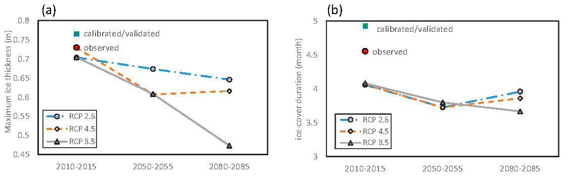
3.1.1. Water Temperature and Ice Cover

The HEAT module was applied to our case study and the results were compared with the measured water temperature values at four locations along the river for four years (2012–2015) and ice thickness at Tugaske Bridge. The results are presented in Figure 4 and Figure 5 which show that the model works well when simulating water temperature (with R2 = 0.88) and ice thickness (with R2 = 0.93).
A local sensitivity analysis was applied to estimate the sensitivity of the water temperature and ice thickness to the forcing data, which included wind speed, cloud cover, air temperature, dew point, flow, and light extinction. The local sensitivity analysis is an effective and widely used method to determine the relative importance of parameters, although it does not account for parameter interactions [33,34,35]. The main advantage of this method is that it requires few model runs whereas global sensitivity analysis is computationally more expensive. Each model input is increased by a defined percentage (here 10%) while holding the other model inputs constant. The sensitivity ε was then assessed using
ε = 1 n i = 1 n ( O x O b a s e ) 2 Δ P
where Obase is the simulated result using the base input, Ox is the simulated result using the perturbed input, ∆P is the difference between base and perturbed input values (10% of the base parameter), and n is the total number of observations. The sensitivity analysis results indicated that air temperature has the most impact on both water temperature and ice thicknesses. Henceforth, for our modelling exercise when using climate models, daily air temperature from PCIC and the average daily historical flow discharge (from 2000 to 2016) seemed sufficient for our assessment. The other forcing data were excluded due to the lack of sensitivity of model results (water temperature and ice thickness) to these factors.
We ran the calibrated/validated model with the downscaled climate data for the same time frame (2012–2015) to verify similarity between model output from sampled data and model output from historical down-scaled climate data. The simulation results followed a similar trend as that shown in Figure 4a. There was good agreement between observed and simulated water temperature using daily maximum and minimum temperature from the CanESM2 RCP 2.6 model which resulted in R2 values of 0.88 and 0.86, respectively. However, in winter 2012–2013, there was some lag between observed and simulated water temperatures.
Ice cover data were sampled with a coarse temporal resolution; therefore, ice cover duration was estimated based on the start and end date of 0 °C water temperature (i.e., the first and last day when the water temperature was 0 °C). Figure 6 illustrates the measured and simulated ice cover duration as well as the average of simulated values using the aforementioned four climate model scenarios. Ice cover periods were over-estimated by three weeks with the calibrated WASP7 model and were underestimated by about 2 weeks with the climate change models, due to the ice cover break up occurring too early.
In Figure 6, the 5-year averaged annual maximum ice thickness and 5-year averaged mean ice-on duration are compared to the observed data. The maximum ice thickness will likely decrease considerably (up to 32.7%) as a result of global warming. The results suggest that the ice cover period will be shorter by up to 12 days in the future, though this is less than the error due to bias. The bias is not due to time of freeze-up but rather, the breakup being simulated early as a result of variability in flow discharge during the freshet. However, this only impacts the simulation of the aforementioned water quality parameters in March and April. Moreover, the water temperature data were collected bi-weekly to monthly rather than daily which may cause some degree of uncertainty in our estimated observed ice cover period.

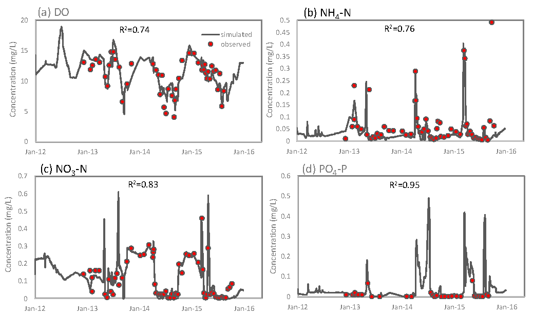
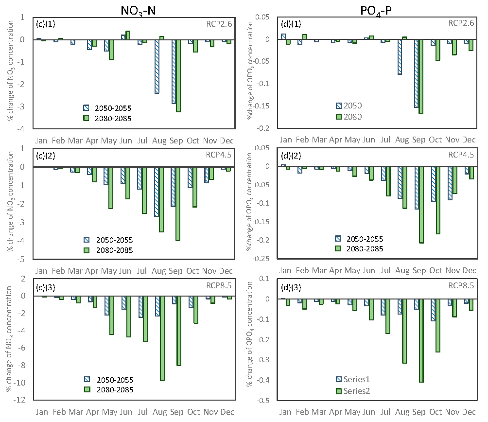
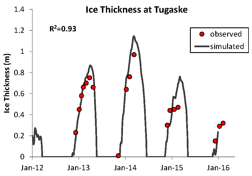
3.1.2. Water Quality

Model calibration output for all parameters is shown in Figure 7 and Figure 8. Calibration (2014–2015) produced a good fit to observed water quality data at the Tugaske and Marquis bridges, which was also the case in the validation (2012–2013). Comparing the simulated concentrations to the measured data yielded R2 values ranging from 0.38 to 0.95. The low correlation coefficient value of 0.38 was found for DO at Marquis, although 90 percent of the data yielded a higher R2 value of 0.78. There were little observed data to compare results for Chl a. Overall, calibration and validation were deemed successful when using the model to predict changes in water quality due to climate change.
Figure 9 compares the measured water quality concentrations and the outputs from the calibrated/validated WASP7 model and from climate change scenarios (i.e., the average of the outputs from all the climate change scenario models). The climate change scenario models were based on the simulated water temperature and ice cover period using historical down-scaled climate data. The 16-year averaged daily flow data at 05JG006 and 05JG013 flow gauges (Figure 1) were used for the climate change model. The 16-year averaged monthly historical concentrations of the water quality parameters including NH4-N, NO3-N, DON, PO4-P, OP, Chl a, and DO were available at the SK05HF026 monitoring station (Figure 1) and 5-year averaged monthly water quality parameter concentrations (NH4-N, NO3-N, DON, PO4-P, OP, and DO) were available at the Ridge Creek and Iskwao Creek monitoring stations (Figure 1) and were used for the climate change model. The mean simulated concentrations matched the measured mean concentrations relatively well.
Figure 10 and Figure 11 show the climate change impact on water quality parameters for 2050–2055 and 2080–2085. The outputs from the RCP 8.5 scenario, which represents the highest greenhouse gas emissions, indicate the largest change in water quality of the system. As might be expected, all the water quality parameters in the 2080–2085 period showed a bigger change than in the 2050–2055 period, except for a few cases (e.g., NH4 in September using the RCP 2.6 scenario).
In general, the mean monthly DO concentrations decrease due to climate change. The reduction in the DO concentrations is not significant in summer while it is pronounced during the ice cover. A minor increase in DO concentrations was predicted in January (about 1%).
Nutrient concentrations were expected to decrease with air temperature increase, although, the magnitude of the changes depends on the model scenarios and seasons. The greatest deviation was observed for nitrogen species with the maximum of 6.71% for NH4-N and 9.79% for NO3-N. In contrast, only a slight change was estimated for phosphorus with the maximum of 0.42%. The results suggest that the highest decrease in the mean monthly concentrations of nitrogen and phosphorus would occur in late summer (September and August).

3.2. Water Management

When flow rates during the ice cover season (November to April) were increased to 6 m3/s and to 14 m3/s in summer, the model output was significantly different from the original, calibrated/validated results (Figure 12). The results revealed that parameters are more sensitive to changes in flow than climate change. DO concentrations are increased in the ice cover periods (December–February), likely due to reaeration of the river, since flows are increased from the Qu’Appelle River Dam, and due to open water, allowing the exchange of gases between the river and atmosphere. However, DO is expected to decline in early spring and late fall. NH4-N and NO3-N generally increase in summer and fluctuate in winter. NH4-N decreased by about 5% in the winter periods when winter flow was increased, while NO3-N slightly increased (about 1.5%–9%) through the winter and into early spring. The phosphate concentrations are also expected to decrease in summer with the greater change in early spring during the freshet.

4. Discussion

4.1. Impact of Increased Air Temperature on Water Quality

Many studies have concluded that water temperature will increase because of global warming [2,3,4,36]. Our modelling results suggest that water temperature will increase between 2010 and either 2050 or 2080 with a corresponding decrease in ice thickness due to warmer air temperatures. Ice cover duration may be up to 12 days shorter by the 2080s but this result is somewhat questionable due to uncertainty in our simulations (Figure 6b). The uncertainty in ice cover duration in this study is mainly attributed to the average flow rate used in our models. Ice breakup is strongly affected by when spring runoff occurs [37]. Historical trend analyses of river and lake ice covers by Magnuson et al. [37] showed similar results of later freeze-up of 5.8 days and earlier break-up of 6.5 days per 100 years.
A reduction in the concentrations of NH4-N, NO3-N, and PO4-P was predicted as a result of warmer water temperatures due to increased air temperatures as a consequences of global warming (Figure 10 and Figure 11). The most significant reduction in the nutrient concentrations were projected during the open-water period relative to the ice covered period. A similar study by Alam et al. [14] also concluded that nutrient concentrations in rivers decline when air temperature increases. The decreases in nutrient concentrations may be a product of increased phytoplankton growth, such that more algae are utilizing more nutrients, and therefore a lower concentration of nutrients remains in the water [14]. A declining trend in total phosphorus concentrations in winter during two decades (1992–2011) was found by Zhang et al. [38] in a shallow reservoir in China, which could be attributed to an increase in grazer abundance. Reduced ice cover duration and ice thickness as presented in the current study, would act favorably towards phytoplankton growth because of better light conditions in winter [39]. Dissolved oxygen concentrations were also projected in this study to decrease in all months, except in January when DO concentrations were predicted to increase slightly (Figure 10). Cox and Whitehead [40] also predicted a reduction in DO concentrations in the River Thames by the 2080s because of reduced saturation concentrations of DO and increased biological oxygen demand.
In contrast to rivers, some climate change studies on the water quality of lakes show that higher water temperatures and increases in oxygen demand promote the release of nutrients from sediments, resulting in more nutrient enrichment of the water column [2,4,39]. The upper Qu’Appelle River is shallow, hence the anoxic conditions which could result in remobilization of nutrients is not a major issue. However, we should note that as the upper Qu’Appelle River flows from Lake Diefenbaker (Figure 1), impact of higher water temperatures on water quality of the lake would consequently affect the water quality of the river system. Such impact was not considered in this current study.

4.2. Impact of Increased Flow

The modelling results are based on water quality parameter concentrations predicted at Tugaske Bridge, at the point where nutrient concentrations and loadings are due to concentrations from Lake Diefenbaker and Ridge Creek. In summer when flow increased to 14 m3/s from the Qu’Appelle River Dam, the increased flow led to an increase in NH4-N and NO3-N concentrations (Figure 12). This likely occurs because with increased flow in the upper Qu’Appelle River from the Dam relative to its base flow, the impact of NO3-N and NH4-N inputs from Ridge Creek was decreased. In contrast, the concentrations of PO4-P decreased because of dilution (Figure 12). The contribution of NH4-N, NO3-N, and PO4-P loads (kg/day) from the Ridge Creek in March and April are on average about 45%, 38%, and 73% of the loading at Tugaske Bridge, respectively. The increase in NO3-N and NH4-N concentrations in the summer period may also be due to higher nitrification and mineralization rates. Increases in nutrient concentrations have been reported in several studies as the result of drought in summer caused by climate change [6,41,42]. For example, increased NH4-N concentrations in a catchment in central Greece were predicted as a result of a reduction in stream dilution capacity due to climate change [6]. Increased flow in the present study led to an increase in DO concentrations, which may be in response to the increased reaeration rate caused by the higher water velocity and flow rate.
Nutrient concentrations fluctuated in winter, when flow from the Qu’Appelle River Dam was increased from base flow to 6 m3/s. The increase in NO3-N concentrations and the decrease in NH4-N in November–January may be due to the increase in DO concentrations which would cause NH4-N oxidation to NO3-N [43]. A small reduction in DO concentrations (about 2%) in October and November may be the result of macrophyte die-off. From the results of this study, it can be inferred that biological activities play a more important role in winter when flow is lower than in summer.

4.3. Future Studies

We assessed the potential impact of increased air temperature, caused by climate change, and increased flow rate, due to flow regulation, on the water quality of the upper Qu’Appelle River. Other factors such as land use change, water quality degradation of Lake Diefenbaker, and climate change impact on catchment nutrient loadings were not considered in this study. Other studies have assessed the impact of climate change on land use change and its consequences on nutrient loadings (e.g., [38,42,44,45,46]. Higher nitrogen and phosphorus loadings to the river may be expected due to increased precipitation caused by global warming especially from agricultural catchments [45,46]. Further studies on the Qu’Appelle River to consider such impacts on the long-term sustainability and security of this water source in Southern Saskatchewan would be beneficial.
Algal dynamics were not considered in this study due to the lack of sufficient measured data for Chl a for validation of the model results. To simulate algal dynamics in the river system, high-frequency and continuous sampling of Chl a would be necessary.

5. Conclusions

In this study, we assessed the future potential impacts of increased air temperature due to climate change and increased flow via water management on the concentrations of nutrients and dissolved oxygen in the upper Qu’Appelle River using the WASP7 model and PCIC climate change models. An important outcome of this study was to develop prediction capacity to assess how changes in flow management and climate change are anticipated to affect downstream changes in water quality. The results show that water quality parameters are highly sensitive to increased flow and air temperature. Warmer water temperatures caused a reduction in the concentrations of nutrients, with a greater decrease in the open water condition and a lower decrease in the ice cover condition. Dissolved oxygen concentrations were predicted to decrease throughout the year except in January when DO concentrations will slightly increase. Based on our study, water quality parameters are more sensitive to flow changes than to climate warming. In summer, increased flow may cause an increase in NH4-N and NO3-N concentrations and a reduction in PO4-P concentrations. Increased meso-eutrophication of Lake Diefenbaker due to climate change would have further impact on the water quality of the upper Qu’Appelle River.
From a water management perspective, the changes in the flow and nutrient regimes of the upper Qu’Appelle River will have implications for water quality in the downstream reservoir Buffalo Pound Lake, a key drinking water source for southern Saskatchewan. Our results indicate that a shift in the nutrient regime may occur primarily due to changes in flows, not climate change. Higher discharges can be brought about by the conveyance of more water from Lake Diefenbaker to Buffalo Pound Lake via the upper Qu’Appelle River. Since Lake Diefenbaker is phosphorus limited, larger transfers of its water downstream may increase the phosphorus limitation in Buffalo Pound Lake. The freshet also has a diluting impact on phosphorus loading in the system. Nitrogen concentrations follow an increasing trend with higher flows, particularly during the summer months due to the high loading from Lake Diefenbaker, which could ultimately enrich Buffalo Pound Lake with additional nitrogen. These conclusions are based on the assumption that the nutrient ratio in Lake Diefenbaker and the nutrient loading from the surrounding landscape in the upper Qu’Appelle Valley will not change substantially in the future. Further study is required to investigate the impacts of land-use changes and changes in the trophic status of Lake Diefenbaker on the upper Qu’Appelle River and ultimately on the aquatic ecosystem of Buffalo Pound Lake.

Acknowledgments

This research was funded by the Canada Excellence Research Chair (CERC) at the University of Saskatchewan’s Global Institute for Water Security. The authors acknowledge the Saskatchewan Water Security Agency and the Saskatchewan Ministry of Environment for providing data used in this study.

Author Contributions

Nasim Hosseini, Jacinda Johnston and Karl-Erich Lindenschmidt conceived the idea and designed the modelling experiments. Nasim Hosseini conducted the simulations and processed the results. Nasim Hosseini and Karl-Erich Lindenschmidt analyzed the results. Nasim Hosseini and Jacinda Johnston wrote the initial draft, and Karl-Erich Lindenschmidt contributed to the writing.

Conflicts of Interest

The authors declare no conflict of interest.

References

  1. Parsons, G.F.; Thorp, T.; Kulshreshtha, S.; Gates, C. Upper Qu’Appelle Water Supply Project: Economic Impact Sensitivity Analysis; Springer: Saskatchewan, SK, Canada, 2012; p. 113. [Google Scholar]
  2. Delpla, I.; Jung, A.V.; Baures, E.; Clement, M.; Thomas, O. Impacts of climate change on surface water quality in relation to drinking water production. Environ. Int. 2009, 35, 1225–1233. [Google Scholar] [CrossRef] [PubMed]
  3. Whitehead, P.G.; Wilby, R.L.; Battarbee, R.W.; Kernan, M.; Wade, A.J. A review of the potential impacts of climate change on surface water quality. Hydrol. Sci. J. 2009, 54, 101–123. [Google Scholar] [CrossRef]
  4. Komatsu, E.; Fukushima, T.; Harasawa, H. A modeling approach to forecast the effect of long-term climate change on lake water quality. Ecol. Model. 2007, 209, 351–366. [Google Scholar] [CrossRef]
  5. Whitehead, P.G.; Barbour, E.; Futter, M.N.; Sarkar, S.; Rodda, H.; Caesar, J.; Butterfield, D.; Jin, L.; Sinha, R.; Nicholls, R.; et al. Impacts of climate change and socio-economic scenarios on flow and water quality of the Ganges, Brahmaputra and Meghna (GBM) river systems: Low flow and flood statistics. Environ. Sci. Process. Impacts 2015, 17, 1057–1069. [Google Scholar] [CrossRef] [PubMed]
  6. Mimikou, M.A.; Baltas, E.; Varanou, E.; Pantazis, K. Regional impacts of climate change on water resources quantity and quality indicators. J. Hydrol. 2000, 234, 95–109. [Google Scholar] [CrossRef]
  7. Van Vliet, M.T.H.; Franssen, W.H.P.; Yearsley, J.R.; Ludwig, F.; Haddeland, I.; Lettenmaier, D.P.; Kabat, P. Global river discharge and water temperature under climate change. Glob. Environ. Chang. 2013, 23, 450–464. [Google Scholar] [CrossRef]
  8. Kienzle, S.W.; Nemeth, M.W.; Byrne, J.M.; MacDonald, R.J. Simulating the hydrological impacts of climate change in the upper North Saskatchewan River basin, Alberta, Canada. J. Hydrol. 2012, 412, 76–89. [Google Scholar] [CrossRef]
  9. Jasper, K.; Calanca, P.; Gyalistras, D.; Fuhrer, J. Differential imapcts of climate change on the hydrology of two alpine river basins. Clim. Res. 2004, 26, 113–129. [Google Scholar] [CrossRef]
  10. Mote, P.W. Climate-driven variability and trends in mountain snowpack in western North America. J. Clim. 2006, 19, 6209–6220. [Google Scholar] [CrossRef]
  11. Wool, T.A.; Ambrose, R.B.; Martin, J.L.; Comer, E.A. Water Quality Analysis Simulation Program (WASP) Version 6.0 Manual. Draft User’s Manual; United States Environmental Protection Agency: Atlanta, GA, USA, 2006.
  12. Cerucci, M.; Jaligama, G.; Amidon, T.; Cosgrove, A. The simulation of dissolved oxygen and orthophosphate for large scale watersheds using WASP7.1 with nutrient luxury uptake. Water Environ. Fed. 2007, 12, 5765–5776. [Google Scholar] [CrossRef]
  13. Huang, J.; Liu, N.; Wang, M.; Yan, K. Application WASP Model on Validation of Reservoir-Drinking Water Source Protection Areas Delineation. In Proceedings of the 2010 3rd International Conference on Biomedical Engineering and Informatics (BMEI), Yantai, China, 16–18 October 2010.
  14. Alam, A.; Badruzzaman, A.B.M.; Ali, M.A. Assessing effect of climate change on the water quality of the Sitalakhya river using WASP model. J. Civ. Eng. 2013, 41, 21–30. [Google Scholar]
  15. Akomeah, E.; Chun, K.P.; Lindenschmidt, K.E. Dynamic water quality modelling and uncertainty analysis of phytoplankton and nutrient cycles for the upper South Saskatchewan River. Environ. Sci. Pollut. Res. 2015, 22, 18239–18251. [Google Scholar] [CrossRef] [PubMed]
  16. Di Toro, D.M.; Fitzpatrick, J.J.; Thomann, R.V. Documentation for Water Quality Analysis Simulation Program (WASP) and Model Verification Program (MVP); United States Environmental Protection Agency: Washington, DC, USA, 1983.
  17. Ambrose, R.B.; Wool, T.A.; Connolly, J.P.; Schanz, R.W. WASP4, a Hydrodynamic and Water Quality Model—Model Theory, User’s Manual, and Programmer’s Guide; EPA-600/3-87/039; Office of Research and Development, United States Environmental Protection Agency: Washington, DC, USA, 1988.
  18. Connolly, J.; Winfield, R. A User’s Guide for WASTOX, a Framework for Moeling the Fate of Toxic Chemicals in Aquatic Environments. Part 1: Exposure Concentration; United States Environmental Protection Agency: Athens, GA, USA, 1984.
  19. Ambrose, R.B.; Wool, T. WASP7 Stream Transport-Model Theory and User’s Guide: Supplement to Water Quality Analysis Simulation Program (WASP) User Documentation; United States Environmental Protection Agency: Washington, DC, USA, 2009.
  20. Cole, T.M.; Buchak, E.M. CE-QUAL-W2: A Two-Dimensional, Laterally Averaged, Hydrodynamic and Water Quality Model, Version 2; Instruction Report EL-95-1; Waterways Experiment Station, US Army Corps of Engineers: Vicksburg, MS, USA, 1995. [Google Scholar]
  21. Tufford, D.L.; McKellar, H.N. Spatial and temporal hydrodynamic and water quality modeling analysis of a large reservoir on the South Carolina (USA) coastal plain. Ecol. Model. 1999, 114, 137–173. [Google Scholar] [CrossRef]
  22. Lindenschmidt, K.-E. Winter Flow Testing of the Upper Qu’Appelle River; Lambert Academic Publishing: Saarbrücken, Germany, 2014. [Google Scholar]
  23. Lindenschmidt, K.-E.; Sereda, J. The impact of macrophytes on winter flows along the Upper Qu’Appelle River. Can. Water Resour. J. 2014, 39, 342–355. [Google Scholar] [CrossRef]
  24. Carpenter, S.R.; Lodge, D.M. Effects of submersed macrophytes on ecosystem processes. Aquat. Bot. 1986, 26, 341–370. [Google Scholar] [CrossRef]
  25. Sand-jensen, K.; Prahl, C.; Stokholm, H. Oxygen release from roots of submerged aquatic macrophytes. Wiley Behalf Nord. Soc. Oikos 2016, 38, 349–354. [Google Scholar] [CrossRef]
  26. Sereda, J. Assessment of Macrophyte Control Options in the Upper Qu’Appelle Conveyance Channel: Nutrient Amendments and Harvesting; Unpublished Report; Saskatchewan Water Security Agancy: Moose Jaw, SK, Canada, 2012. [Google Scholar]
  27. Tolson, B.A.; Shoemaker, C.A. Dynamically dimensioned search algorithm for computationally efficient watershed model calibration. Water Resour. Res. 2007, 43, 1–16. [Google Scholar] [CrossRef]
  28. Matott, L.S. OSTRICH: An Optimization Software Tool; Documentation and User’s Guide; Univisity of Buffalo: Buffalo, NY, USA, 2008. [Google Scholar]
  29. Murdock, T.Q.; Spittlehouse, D.L. Selecting and Using Climate Change Scenarios for British Columbia; Pacific Climate Impacts Consortium: Univisity of Victoria, Victoria, BC, Canada, 2011; Volume 39, p. 4. [Google Scholar]
  30. Taylor, K.E.; Stouffer, R.J.; Meehl, G.A. An overview of CMIP5 and the experiment design. Bull. Am. Meteorol. Soc. 2012, 93, 485–498. [Google Scholar] [CrossRef]
  31. McKenney, D.W.; Hutchiinson, M.F.; Papadopol, P.; Lawrence, K.; Pedlar, J.; Campbell, K.; Milewska, E.; Hopkinson, R.F.; Price, D.; Owen, T. Customized spatial climate models for North America. Bull. Am. Meteorol. Soc. 2011, 92, 1611–1622. [Google Scholar] [CrossRef]
  32. Hopkinson, R.F.; Mckenney, D.W.; Milewska, E.J.; Hutchinson, M.F.; Papadopol, P.; Vincent, A.L.A. Impact of aligning climatological day on gridding daily maximum-minimum temperature and precipitation over Canada. J. Appl. Meteorol. Climatol. 2011, 50, 1654–1665. [Google Scholar] [CrossRef]
  33. Tang, Y.; Reed, P.; Wagener, T.; van Werkhoven, K. Comparing sensitivity analysis methods to advance lumped watershed model identification and evaluation. Hydrol. Earth Syst. Sci. 2007, 11, 793–817. [Google Scholar] [CrossRef]
  34. Razavi, S.; Gupta, H.V. What do we mean by sensitivity analysis? The need for comprehensive characterization of “global” sensitivity in earth and environmental systems models. Water Resour. Res. 2015, 51, 3070–3092. [Google Scholar] [CrossRef]
  35. Saltelli, A.; Ratto, M.; Tarantola, S.; Campolongo, F. Sensitivity analysis for chemical models. Chem. Rev. 2005, 105, 2811–2827. [Google Scholar] [CrossRef] [PubMed]
  36. Park, J.Y.; Park, G.A.; Kim, S.J. Assessment of future climate change impact on water quality of Chungju Lake, South Korea, Using WASP Coupled with SWAT. J. Am. Water Resour. Assoc. 2013, 49, 1225–1238. [Google Scholar] [CrossRef]
  37. Magnuson, J.J.; Robertson, D.M.; Benson, B.J.; Wynne, R.H.; Livingstone, D.M.; Arai, T.; Assel, R.A.; Barry, R.G.; Card, V.; Kuuisisto, E.; et al. Historical trends in lake and river ice cover in the Northern Hemisphere. Science 2000, 289, 1743–1746. [Google Scholar] [CrossRef] [PubMed]
  38. Zhang, C.; Lai, S.; Gao, X.; Xu, L. Potential impacts of climate change on water quality in a shallow reservoir in China. Environ. Sci. Pollut. Res. Int. 2015, 22, 14971–14982. [Google Scholar] [CrossRef] [PubMed]
  39. Pettersson, K.; Grust, K.; Weyhenmeyer, G.; Blenckner, T. Seasonality of chlorophyll and nutrients in Lake Erken—Effects of weather conditions. Hydrobiologia 2003, 506–509, 75–81. [Google Scholar] [CrossRef]
  40. Cox, B.A.; Whitehead, P.G. Impacts of climate change scenarios on dissolved oxygen in the River Thames, UK. Hydrol. Res. 2009, 40, 138. [Google Scholar] [CrossRef]
  41. Murdoch, P.S.; Baron, J.S.; Miller, T.L. Potential effects of climate change on surface-water quality in North America. J. Am. Water Resour. Assoc. 2000, 36, 347–366. [Google Scholar] [CrossRef]
  42. Wilby, R.L.; Whitehead, P.G.; Wade, A.J.; Butterfield, D.; Davis, R.J.; Watts, G. Integrated modelling of climate change impacts on water resources and quality in a lowland catchment: River Kennet, UK. J. Hydrol. 2006, 330, 204–220. [Google Scholar] [CrossRef]
  43. Dodson, S.I. Introduction to Limnology. J. N. Am. Benthol. Soc. 2004, 23, 661–662. [Google Scholar] [CrossRef]
  44. Tu, J. Combined impact of climate and land use changes on streamflow and water quality in eastern Massachusetts, USA. J. Hydrol. 2009, 379, 268–283. [Google Scholar] [CrossRef]
  45. Arheimer, B.; Andreasson, J.; Fogelberg, S.; Johnsson, H.; Pers, C.B.; Persson, K. Climate change impact on water quality: Model results from southern Sweden. AMBIO 2005, 34, 559–566. [Google Scholar] [CrossRef] [PubMed]
  46. Tong, S.T.Y.; Chen, W.L. Modeling the relationship between land use and surface water quality. J. Environ. Manag. 2002, 66, 377–393. [Google Scholar] [CrossRef]
Figure 1. Map of the upper Qu’Appelle River. The lower Qu’Appelle River flows out of Buffalo Pound Lake.
Water 09 00199 g001
Figure 2. Upper Qu’Appelle River flow between 2012 and 2015 with indicated ice cover periods and 2012–2013 winter flow test.
Water 09 00199 g002
Figure 3. Range of concentrations occurring for water quality parameters at the upstream boundary condition used in the WASP7 model for the upper Qu’Appelle River. n indicates the number of observations.
Water 09 00199 g003
Figure 4. Simulated and measured water temperature at (a) Tugaske; (b) Marquis; (c) Brownlee; and (d) HWY#2.
Water 09 00199 g004
Figure 5. Daily simulated ice thickness at the Tugaske Bridge.
Water 09 00199 g005
Figure 6. Climate change impact on (a) maximum ice thickness and (b) ice-on duration.
Water 09 00199 g006
Figure 7. Calibration (2014–2015) and validation (2012–2013) results for simulated versus observed water quality data (a) DO (dissolved oxygen); (b) NH4-N; (c) NO3-N; and (d) PO4-P at Tugaske Bridge.
Water 09 00199 g007
Figure 8. Calibration (2014–2015) and validation (2012–2013) results for simulated versus observed water quality data (a) DO; (b) NH4-N; (c) NO3-N; and (d) PO4-P at Marquis Bridge.
Water 09 00199 g008
Figure 9. Measure and simulated water quality parameter concentrations using calibrated/validated model and climate change scenario models (a) DO; (b) NH4-N; (c) NO3-N; and (d) PO4-P.
Water 09 00199 g009
Figure 10. Percent change in water quality parameter concentrations for DO and NH4-N, due to climate change scenarios (Representative Concentration Pathway) (1) RCP 2.6; (2) RCP 4.5; and (3) RCP 8.5 at the Tugaske location.
Water 09 00199 g010
Figure 11. Percent change in water quality parameter concentrations for NO3-N, and PO4-P due to climate change scenarios (1) RCP 2.6; (2) RCP 4.5; and (3) RCP 8.5 at the Tugaske location.
Water 09 00199 g011
Figure 12. Changes in water quality parameters (a) DO; (b) NH4-N; (c) NO3-N; and (d) PO4-P due to flow increase for the RCP 8.5 scenario at the Tugaske location.
Water 09 00199 g012
Table 1. Water quality monitoring stations and the number of observations used for calibration and validation.
Station NamesNumber of Observations from January 2012 to December 2015
DONH4-NNO3-NPO4-PChl a
Qu’Appelle River at Marquis Bridge798080397
Qu’Appelle River at Keeler5 *5555
Qu’Appelle River at Brownlee532222
Qu’Appelle River below Eyebrown Bridge46620
Qu’Appelle River at Tugaske Bridge646464311
Note: * January 2013 to April 2013.

