Article

Economic Insight from Utah’s Water Efficiency Supply Curve

1
Department of Applied Economics, Utah State University, Salt Lake City, UT 84112, USA
2
Undergraduate Researchers, Utah State University, Salt Lake City, UT 84112, USA
*
Author to whom correspondence should be addressed.
Water 2017, 9(3), 214; https://doi.org/10.3390/w9030214
Submission received: 27 October 2016 / Revised: 19 January 2017 / Accepted: 6 March 2017 / Published: 13 March 2017

Abstract

:
Across the western US, growing populations and urbanization along with environmental demands and a changing climate have strained water allocation mechanisms originally designed to provide water to agriculture. This paper provides a methodology, using Utah as an example, for examining the options for new water supply via conservation, interpretable by policymakers, water agencies, and water users. Findings indicate that the largest potential water savings, at the lowest cost, are in agriculture and outdoor residential water use, where more efficient applications can maintain the acreage of crops and lawns at current levels while dramatically reducing use.

1. Introduction

Acquiring sufficient water supply to meet demand has been an ongoing concern in the western US. Growing urban demand has strained limited water supplies and increased pressure on the institutions governing transfers to allow more water to move from agriculture to other uses [1]. Additionally, rising demand for environmental flows and associated protections of riparian ecosystems has placed constraints on both new and existing supplies [2,3]. The Endangered Species Act (1973), National Environmental Policy Act (1970), and wetland protections under the Clean Water Act (1972) are examples of the types of restrictions placed on existing and new water supply options, limiting where, when, and how much water can be removed from natural systems. Finally, climate change will likely change the variability, amount and type of precipitation, and subsequently the availability of water [4].
In a well-functioning market, shortages are generally addressed by increasing prices, which spur conservation and the development of additional supply. However, the allocation of water in the western United States is determined under the rules of the appropriative rights doctrine, which assigns property rights to water by the historic order of request. This is referred to as “first-in-time, first-in-right” because senior appropriators receive their water allocation first in times of shortage. Agriculture has historically been the primary use of water, and most senior rights rest with irrigators. Like other western states, a majority of Utah’s developed water supply was and continues to be used in agriculture.
Market price mechanisms do not generally exist for water as in other goods. The institutional arrangements associated with the appropriative rights doctrine determine that many water users do not pay the full scarcity cost of the water they use. Moreover, these institutional arrangements also generally place restrictions on water sales, especially those which move water out of agricultural production [2]. These barriers to the transfer of water rights can lock water resources in low-value uses, and create scarcity in sectors that would otherwise simply purchase water rights. Given these institutional restrictions, it is worthwhile to examine to what extent water scarcity can be addressed by reducing demand and increasing supply, and the relative costs of different approaches.
A lack of water markets with clear price signals creates difficulty in evaluating the cost effectiveness and social value of water supply development projects and other policy proposals. For example, in the state of Utah, two proposed development projects, the Bear River Development Project and the Lake Powell Pipeline, are currently the subject of public debate. Although the costs of these projects can be estimated via conventional techniques, the lack of price signals from water markets obfuscates the cost of other policy options that could provide an equivalent supply of water. Estimating the cost of conserving water, rather than developing new supplies, offers one approach for examining the opportunity cost of development projects. Furthermore, conservation options may not be priced into markets where they exist because irrigators are often not able to sell conserved water. When agricultural irrigators, and to a lesser extent residential irrigators, do not see direct monetary benefits from conserving water, they have little incentive to do so. In agriculture, conserved water may not be retained by the irrigator who conserved it, and often cannot be sold into other sectors [
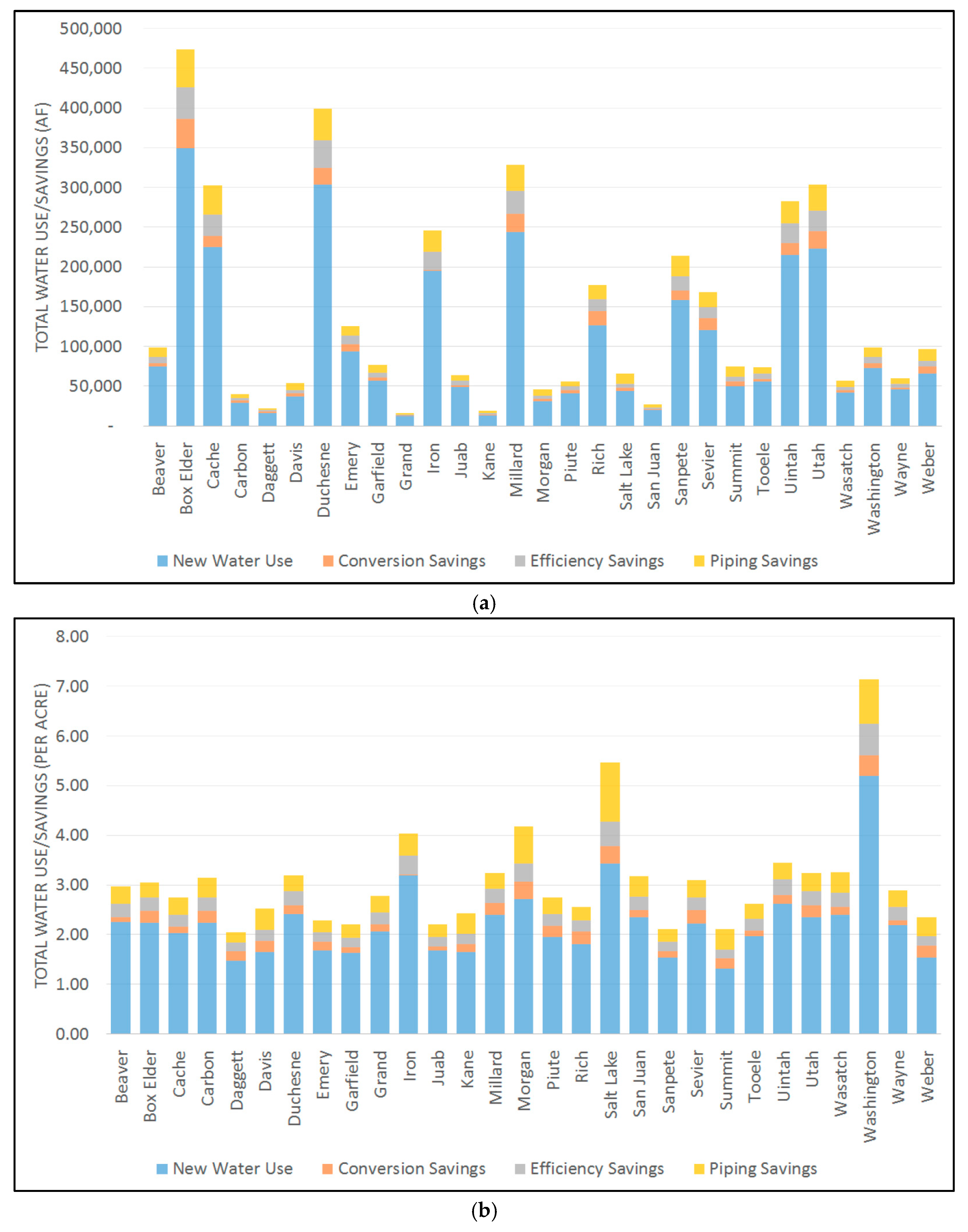
5]. Irrigation also represents the two largest categories of water use in the state, with agriculture accounting for 82% and residential outdoor accounting for 6% of total water use [6]. Therefore, we hypothesize that the largest conservation savings at the lowest prices will come from agricultural and urban irrigation.
The key contribution of this paper is to provide a “big picture” assessment of the costs associated with expanding the water supply though various policies and technologies. Although our estimates for any single conservation method should not be viewed as authoritative, we provide a general methodology for organizing information on the relative costs of various policies designed to conserve water supplies in Utah. The estimates provided herein can be easily updated and expanded as better information becomes available and new policies or technologies are developed. Our methodology is similar to the approach taken by Granade et al. in their report Unlocking Energy Efficiency in the U.S. Economy [7]. This report provided a clear graphical representation for a comparative assessment of different technologies in terms of cost and the amount of energy savings. This paper constructs a similar representation for a water efficiency supply curve to that of [8]. However, relative to electricity, water is a more localized commodity due to its high transportation cost, so we chose to focus on a constrained geographic area by developing estimates for the state of Utah. This is the first paper we are aware of to provide a direct comparison of conservation measures at the state and sub-state level interpretable by policymakers, water agencies, and water users.
Data is gathered on six potential categories for water conservation: residential indoor, residential outdoor, commercial, wastewater, agriculture, and water resource development. Within each area, multiple conservation technologies were selected based on their relevance to Utah water conservation. While not as comprehensive as other estimates, (e.g., [9]), this work is designed to better illustrate the economic tradeoffs and barriers to water conservation. Current water use in Utah is estimated at around 5.15 million acre-feet (AF) per year [
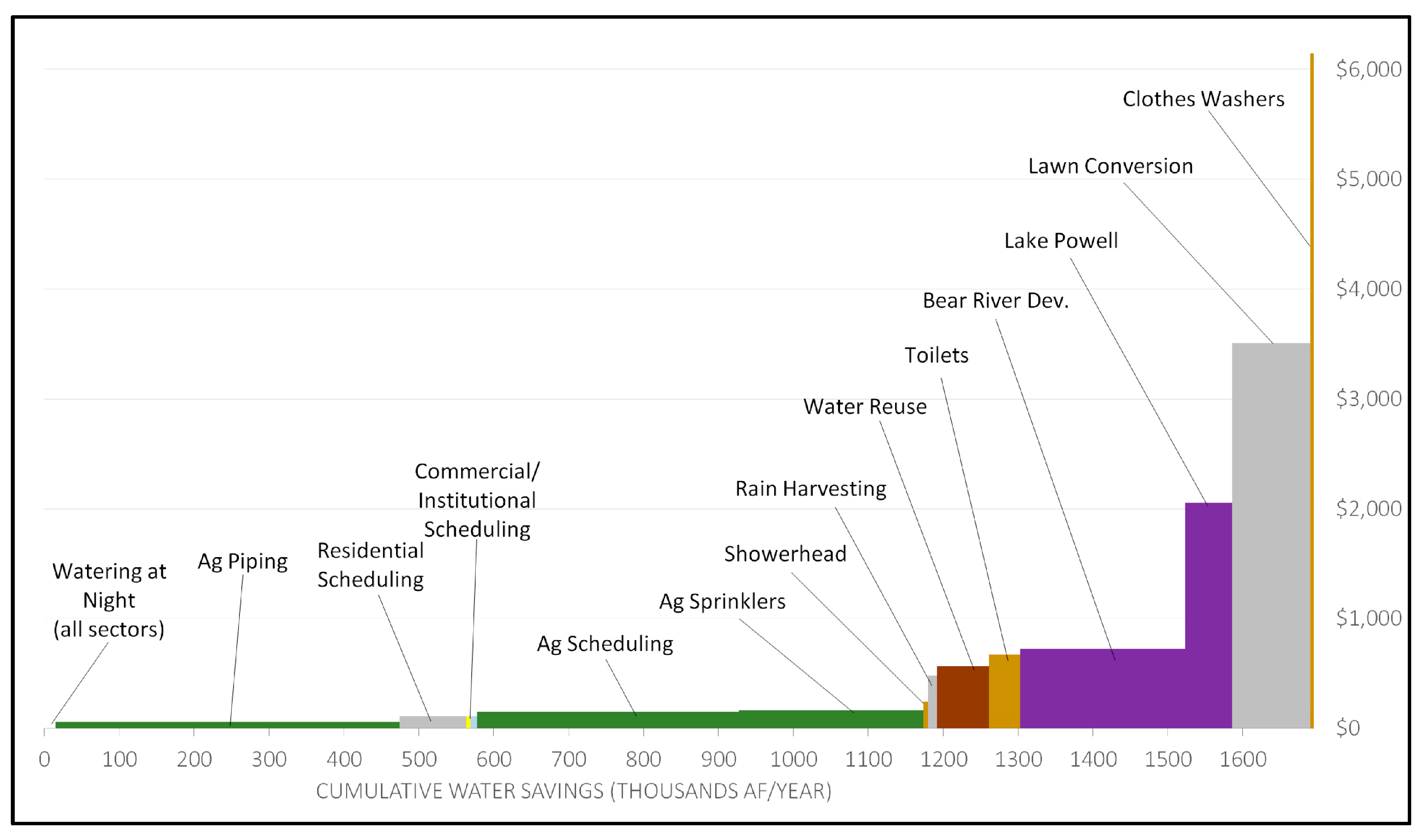
6], and in total the measures we consider could provide up to 1.7 million AF through conservation and new supply development. The cost of providing this water varies dramatically, from behavioral changes such as watering at night that cost nothing in monetary terms, to expensive landscape conversion costing around $3508 per AF saved.
Findings indicate that the largest potential water savings, at the lowest costs, are in agriculture and outdoor residential water use, where more efficient use of water can maintain acreage of crops and lawns at current levels while dramatically reducing use. Cost estimates for development projects, such as dams, are higher than many conservation technologies, even as these projects are seriously considered as viable supply options for the state of Utah. While conservation potential exists in agriculture, it is important to acknowledge that significant barriers to conservation exist, and even if conservation methods were adopted, they might not result in the movement of water to high value uses. For instance, subsidies for irrigation efficiency may not lead to reduced water usage, as the conserved water is applied to additional agricultural land and reduces return flows [10].

2. Methodology

We estimate a water efficiency supply curve for various water conservation measures in the state of Utah. The correct metric for measuring water use efficiency, especially in agriculture, is the subject of debate [11] and efficiency savings estimates that fail to account for return flows to the hydrologic system may overestimate actual water savings [12]. To address these issues, we define water efficiency as any technology, behavior, or system adjustment that conserves water without decreasing the direct benefits provided by the water in its original use. Thus, when the conservation of water decreases directly used return flows, savings are adjusted to the consumptive use only. This definition separates water supplied through conservation from water supplied via sales, transfers, or reallocations. We offer a comparison of various conservation approaches based on engineering and behavioral savings estimates. These comparisons can be used as a tool for policymakers to understand both the options for water conservation and the barriers that raise transaction costs and prevent the implementation of many seemingly low-cost conservation approaches.
To organize potential conservation measures, we designate six categories: residential indoor, residential outdoor, commercial, wastewater, agriculture, and development. Within each category we select a number of important water conservation measures. Table 1 provides a listing of the measures considered by each category. Overall we estimate the conservation potential and cost savings of 15 measures which were selected from a broader survey of potential measures. The list is not meant to be comprehensive. Instead, efforts were made to include measures that were widely discussed in the popular press, by professionals in the field, and in various disciplinary literatures. Because this project primarily focuses on Utah, some measures are specific to the potential water supply available in the state.
Research on each conservation approach was conducted to create an estimate of the quantity of water that could be conserved, and the cost of conserving that water. In economics, the short term is characterized by the adjustment of factors to provide the most efficient outcome given a fixed method of production. In the long term, the production process itself can be modified, changing the relationship between the factors of production. The majority of the measures considered are long-run, requiring an up-front capital investment to conserve a quantity of water for some period. For consistency, we generate a cost per AF per year. Given a project producing a quantity, Q, per year for a total cost K, lasting a number of years, t, we apply the annuity formula to find the per-year fixed cost, C 0 :
C 0 = r · K 1 ( 1 + r ) t
where r is the interest rate assumed across all approaches to be 5%. We add any annual cost, C p , such as maintenance, to arrive at the per year cost, C = C 0 + C p . We then define the per AF cost as κ = C Q .
The project cost is estimated by assessing all direct project expenditures, but excludes the opportunity cost of using water in a particular way. In general, this is straightforward: an approach to conserving water may require investment in technology, training, and construction, and all these costs are included. The alternative uses to which the water could be put, however, are excluded—these are the uses for which the conserved water can be applied, i.e., the demand curve. Environmental costs that are directly incurred, like payments made for required environmental mitigation, are included but costs that will not be directly borne are not. This approach is potentially problematic when conserving water creates large direct but unpriced environmental costs, for example a large dam development makes additional water available at the expense of ecological benefits provided by a flowing river. However, for practical reasons this approach is necessary: unpriced environmental benefits require empirical estimation beyond the scope of this paper. We return to environmental impact in detail in the discussion section of the paper.
We estimate the cost and useful life of the equipment as well as the amount of water made available by each conservation method using various sources including the available academic literature, governmental reports, and interviews with experts. The methodology and sources used for estimating the cost of each conservation method are described in detail in the Results section. To estimate the amount of water made available, technologies are scaled based on the total number of potential adopters. The baseline assumption is that any technology can be supplied at its estimated cost to the entire population of users who have not yet adopted it. The supply curve is constructed using our estimates of per-AF cost and the total potential quantity saved: the per-AF cost is plotted on the y-axis and the quantity conserved on the x-axis. Given n-conservation methods, we order them such that: κ 1 κ 2 κ n . Then we plot them, such that:
( x , y ) = ( j i i Q j , κ i ) ,   i = 1 , 2 , , n
For the ease of interpretation and calculation, conservation methods in this paper will form a step function. However, this method is generalizable to methods with upward sloping cost functions, with Equation (2) modified to sum continuous functions horizontally.

3. Results

For each of the six conservation categories, we describe data sources and the approach for calculating the cost and expected savings from adoption. Counterfactual scenarios examine adoption rates at 100%, as a means of showing the full water supply potential for each conservation method. We provide overall estimates for the state of Utah, and also geographically break the state into three regions: eastern, northern, and southwestern, as shown in Figure 1. Because water transportation potential is limited, these regional efficiency curves provide a more accurate projection of potential savings and costs.

3.1. Residential Indoor

Only about 4% of Utah’s water is used in a residential indoor setting [6]. Although water savings in this area appear limited, we investigate the potential for water conservation through the use of low-flow toilets, reduced-flow showerheads, and high-efficiency clothes washers. We model a 100% switchover scenario in which all possible appliances are converted to efficient models. This represents a best-case scenario for water savings, and avoids modeling the actual adoption rates under different incentive programs.
The Energy Policy Act mandated in 1994 that all new toilets should not exceed a maximum of 1.6 gallons per flush (gpf). Utah adopted these measures in 1991 [13]. To calculate the potential for water savings via conversion to low-flow toilets, we first assume pre-1990 fixtures use 6 gallons per flush [6] (p. 45). We also use data from a nationwide survey, the Residential End Uses of Water (REUW), conducted in 1999 by the American Water Works Association [14] and updated in 2016 [15]. Housing unit counts, including multifamily residential, are taken from the American Community Survey conducted by the US Census Bureau [16]. From the REUW we assume there are 2.27 toilets per housing unit [14] (p. 96) and that 37% of homes already have low-flow toilets [15] (p. 10). Multiplying these estimates by the total number of housing units gives an approximation of the stock of toilets that exist in Utah.
Applying an average of 5.05 flushes per day, per person [14] (p. 96), we counterfactually estimate a 100% switchover scenario where all standard toilets are converted to low-flow. We estimate a total conservation potential of 41,667 AF per year and the cost of a low-flow fixture replacement to be $180, plus installation costs of $110 for two hours of labor [9] (pp. 126–127), giving a cost estimate of $673 per AF. Our cost estimate is similar to the $200 for combined parts and labor found for a low-flow toilet replacement program conducted in Utah [13]. We chose to use the more expensive estimate because it was more transparent about the applicability of methods beyond the study at hand.
The Energy Policy Act mandated maximum flow rates for showerheads at 2.5 gallons per minute (gpm) while older models use between 3.5 and 8 gpm. We use an estimate of 5 gpm for the older models. Data from the REUW indicates that the average shower duration is 6.8 and 8.5 min long for older and newer models, respectively [14] (p. 171). We assume a shower frequency of 0.75 showers per person per day and 1.95 showerheads per home [15] (p. xxvii and 70). Eighty percent of homes are estimated to have already installed efficient showerheads [15] (p. 10). If 100% of high-flow showerheads were converted to low-flow, and adjusting for the fact that showers with low-flow heads are longer, we estimate a potential of 5693 AF per year of water savings. Average costs were estimated from a range of 25 different models to be $24.50 per showerhead and installation required 30 min of labor [9] (p. 128), leading to an estimate of $241 per AF.
Unlike toilets and showerheads, which were required to be upgraded under the Energy Policy Act, there have been no mandated technology standards for residential clothes washers. However, in 1992, the United States Environmental Protection Agency established the Energy Star program to promote a standard for energy efficient products. Gleick et al. [9] (p. 53), estimated that about 73% of households in California own washing machines and, based on industry information, estimated a useful life of 12 years for new washing machines. These estimates are applied to Utah due to a lack of specific state estimates in the literature. Forty-six percent of homes are estimated to have already installed high-efficiency (HE) washers [15] (p. 10). Standard flow washers were estimated at 36.1 gallons per load and HE at 24.2 gallons per load, with each house doing 0.96 cycles per day [9] (p. 52). We calculate a potential water savings of 4,804 AF for the state under a 100% switchover scenario. For HE washing machines, the replacement cost on average is about $587 and applying 2 h of installation at $55 per hour [9] (p. 125), gives a cost of implementation of $6145 per AF. Table 2 shows the number of fixtures or appliances changed, along with estimates of the cost and water savings.

3.2. Residential Outdoor

We examine four methods for conserving residential water used for irrigating turf and other plants: rainwater harvesting, watering at night, irrigation scheduling, and partial turf conversion. Rainwater harvesting utilizes barrels to collect and store water for residential irrigation. Water collection estimates for April–October were created using rain collection studies for Utah cities by the Utah State University Extension [16]. The average water gathered was then multiplied by the number of houses [17]. A wide range of costs and options exist for water barrels, ranging from $50 to over $1000 [16]. Because there are not clear conservation benefits to acquiring more expensive barrels, we use the lowest cost of a 50-gallon barrel and the relevant parts of $75 found at Home Depot. A 20-year useful life for the barrel was assumed. The average cost per AF across Utah was estimated at $482.
The other conservation measures in this category all build on each other by reducing losses in irrigating outdoor turf: subsequent methods only save water remaining after implementation of the methods adopted prior. Total water use estimates for residential irrigation come from the Utah Division of Water Resources [18]. Around 11.2% of Utah homes are estimated to use an alternative, non-turf, groundcover [19] (p. 24). The remaining homes could first switch to watering at night, a step that 46% of homes have already undertaken [19] (p. 28) and which saves around 5% of total irrigation [20]. This is a costless measure expected to save 12,666 AF per year. Homes also have the potential to utilize irrigation scheduling controllers, provided they are one of the 73.3% of Utahans with in-ground irrigation systems [19] (p. 27); users who hand water, colloquially referred to as hose-draggers, often irrigate much more efficiently already. We assume 10% of homes already use the scheduling feature of their irrigation controller and scheduling to irrigate less in wetter months is estimated to save 30% of total irrigation water over the season [21]. Controller costs are estimated at between $40 and $250, based on commercially available systems, with a useful life of 20 years. Turf can also be converted to less water intensive plants. We estimate the savings of turf conversion at 28.6%, which provides overall savings of a turf conversion and scheduling project consistent with an estimate of 50% from [21], and is similar to an estimate of net 30% water savings for conversion from [22] (p. 60). The cost of conversion is estimated at $1.37–$1.93 per square foot [22] (p. 51), with the assumed conversion being around 2126 square feet [22] (p. 11). Table 3 shows the potential savings and costs of outdoor conservation aggregated over all of Utah.

3.3. Commercial

We considered three categories for commercial water use: commercial, institutional, and industrial. In Utah, commercial uses were 97,000 AF per year, institutional uses were 85,000 AF per year, and industrial uses were 26,000 AF per year [6] (p. 4). Industrial savings were excluded because they amounted to little water spread across many disparate industries. For commercial and institutional, we consider only efficiency improvements from outdoor landscaping: watering at night and improved scheduling. Commercial users are assumed to use 20.06% of water for landscaping, an estimate for office buildings, and institutional users are assumed to use 36.77%, an estimate for schools [23] (p. B-5 and B-7). Institutional savings for the two measures total 9054 AF for the state, and commercial conversion saves 5637 AF. Per AF cost estimates for scheduling, taken from residential estimates, average $111 per AF for the state as a whole.

3.4. Wastewater

We estimate the potential for increased supply through wastewater reuse in Utah. Stonely et al. [24] (p. 35) estimate that about 50% of water from wastewater treatment plants (WWTP) that have total containment pools can be reused while about 40% from all other types of WWTPs can be reused. Recycled wastewater directly reduces return flows because a portion is consumed consumptively and does not return to the stream. We assume that wastewater is used for outdoor irrigation where the consumptive rate is estimated to be between 31% and 57% [25] (p. 42). We apply these rates to the water available for reuse from plants that do not have total containment pools. Plants with total containment pools have no return flows and therefore 100% of the water available for reuse was assumed to be a new supply.
We estimate the potential for water savings under both a high (57%) and low (31%) assumption for the consumptive rate of cities. Applying these rates to the estimates of current volumes available for reuse in Stonely et al. [24] (p. 35), we find the potential savings for Utah from water reuse is between 53,115 AF and 85,230 AF, of which we use a simple mean for display on the efficiency curves.
Due to confidentiality concerns expressed by Utah wastewater treatment plants, we estimate the costs associated with water reuse using the case of the Denver Water Recycling Project: the cost of the facility was approximately $80 million, and the cost of water distribution infrastructure was an additional $40 million, with yearly maintenance costs estimated to be $2.3 million [26] (p. 6). Assuming a useful life of 25 years [26], the fixed costs were amortized and then added to the yearly maintenance figure. Applying these costs to the yearly capacity of the plant, 19,027 AF, yields an estimate of $568/AF, consistent with the cost estimates reported in Stonely et al. [24] (pp. 73–74). Assuming an approximately constant return to scale production technology for water treatment facilities enables us to apply this cost estimate to the potential for water treatment plants in Utah.

3.5. Agriculture

In 2012 more than 67% of cropland in Utah was irrigated, and nearly 69% of harvested acres were hay or alfalfa [27]. Water use and potential savings vary across Utah based on climate and irrigation technology. Total agricultural water use by county from the United States Geological Survey [28] includes the amount of water used in surface and sprinkler irrigation. Surface, or flood, irrigation is typically less efficient than sprinkler irrigation. While northern Utah produces a wider variety of crops than southern Utah, there is no consistent pattern across the state in terms of irrigation method. Only 42% of agricultural water in Cache County is applied via surface irrigation while neighboring Box Elder County in the same watershed and with similar climate and crops applied 68% of water via flood irrigation [28]. These differences guided our decision to calculate agricultural water savings estimates on a per-county basis.
We estimate the costs and water availability of three types of agricultural conservation: conversion of surface irrigation to sprinklers, improved irrigation scheduling, and canal piping. Based on conversations with Utah State University extension specialists, we used estimates from the literature that flood irrigation is 70% efficient, center-pivot sprinklers are 80% efficient [29] (p. 52), and that the change in return flows is negligible. Thus, the potential savings from the conversion to sprinklers depend on the total irrigation water use for each county, as well as the method of application. The cost of a pivot system actually implemented by the USU extension was $716 per acre, with total amortized cost plus maintenance at around $58.29 per year [30]. These costs are similar but less than estimates in North Dakota ($1144/acre) [31] and Alabama ($1223/acre) [32]. We use the Utah estimate for the Utah efficiency curves, but note that the estimates from the literature would likely be more suitable for constructing curves elsewhere in the United States. Cost per AF of savings ranges from $67 in Washington County to $241 in Daggett County. Savings exceed 247,000 AF for all of Utah.
We estimate that improved irrigation scheduling can increase efficiency by 13% [33] via [34] (p. 46), and assume that 20% of irrigators have already adopted this technology [34] (p. 47). Both these estimates come from California and will be conservative in terms of efficiency gains; Utah is likely to have more gains from better scheduling and less current adoption due to lower valued agriculture. Savings are calculated after assuming the conversion to sprinkler technology has taken place: sprinkler savings are not available to be saved through scheduling. Costs of implementation are estimated at $15 per acre yearly [35] via [34] (p. 48) and the technological cost of the system itself is $20–30 per acre [34] (p. 48). Costs range from $63-$228/AF saved and total savings exceed 349,000 AF for all of Utah.
Canal piping saves water by reducing leakage and evaporation. Costs and savings are estimated after assuming that both conversion and efficiency investments have taken place. Currently projects in Utah apply for federal funding from the Bureau of Reclamation for canal piping funding. We use water savings from these projects, which range from 20% to more than 40%, as a basis for estimating the additional conservation available. Data shows each project’s estimated cost, the length of canal being piped, the flow of water through the pipe, and its estimated savings [36]. The state of Utah has approximately 1500 canal companies, and they are generally private; to our knowledge there is not a complete accounting of Utah’s canals and ditches. Thus, we estimate water diversions by taking the agricultural diversions by county, after assuming both conversion and efficiency investments have taken place, and divide by the number of canal companies [37]. We assume each canal company has a single ditch that preliminarily diverts its water before moving it into smaller ditches, feeders, and laterals. We estimate the water savings and canal length by running a linear regression on the BOR data [36], to estimate the relationship between water savings and quantity of diversion, and canal length and quantity of diversion. Total estimated water savings for the state exceed 459,000 AF, at costs ranging from $43–$78 per AF saved.
Figure 2a shows the potential savings for each county in Utah. The full column represents total current water use, which is the sum of the savings and projected new water use after the conservation savings are implemented. Figure 2b shows the per-acre savings in the same manner. The contrast between the figures shows that counties with the most potential savings per acre are not necessarily the highest water savers. Per-acre water savings are determined by per acre water use, which is a function of the type of irrigation used as well as other county specific factors. Overall water savings are related both to per-acre savings as well as the number of acres in production. Washington County has the largest potential per-acre savings, but because its agriculture base is limited, the total volume of potential savings is lower. Agricultural savings are not evenly distributed across the state, with the largest overall volumes in the far north and east, where there is more irrigated agriculture.

3.6. Development

We examine two large potential development projects to bring water to Utah cities and farmers: the Lake Powell Pipeline in southwestern Utah and the Bear River Project in northern Utah. For each estimate we used cost reports commissioned by engineering firms [38] (p. 12-6); [39] (p. 5-3 and 5-5). These costs may underestimate construction budget overruns and typically only provide present value costs, which obscures assumptions about cost escalation and discounting. However, because the projects are still in the early planning stages, these reports represent the best available information. To these costs we add environmental costs where construction was expected to lead to direct payments for environmental mitigation. For the Bear River Project, environmental mitigation costs were not included in project costs, but were estimated in the consultant report and are included using the “typical” wetland mitigation cost estimates [38] (pp. 10–27). These estimates were then used to calculate a mitigation to capital expenditure ratio to apply to the Lake Powell Pipeline; to our knowledge, mitigation cost estimates do not exist. Land acquisition costs for the Lake Powell Pipeline were not estimated and are not included. For the Bear River Development the capital estimates include pipeline right-of-way land acquisition costs, and our estimate adds reservoir land acquisition costs as well [38] (pp. 10–31). For both projects, an 8% operation and maintenance budget and 30-year life were assumed. Table 4 shows the expected water generated by each project, and estimated overall costs by category and per AF.

3.7. Water Efficiency Supply Curves

Figure 3 shows the water efficiency supply curve for the state of Utah. The curve shows savings totaling nearly 1.7 million AF. With costs ranging from $0 to over $6000 per AF conserved. The largest savings come from agriculture, due in part to its large proportion of water use in Utah. The curve provides a good visual representation of where water supply could come from via conservation. Another useful application is in examining regional conservation potential within Utah. We separate Utah into three geographically distinct regions (shown in Figure 1): northern Utah, fed by tributaries to the Great Salt Lake; eastern Utah, in the Green River/Colorado River basin; and southwestern Utah, which is supplied by the Virgin River and Sevier Lake systems. Table 5 provides a detailed breakdown of the savings and cost estimates for each measure, for Utah as a whole and for each of the three regions.
Figure 4a–c show the water conservation potential of each of the three regions. All areas see large potential savings from agricultural efficiency measures and relatively low costs. Northern Utah has the most potential savings, and due to its relatively high urban population, has more savings from residential conservation measures relative to the other regions. Eastern Utah has a small population and no potential supply development projects; water conservation in this region will come almost exclusively from agriculture. Southwestern Utah also has relatively low potential for residential conservation, leaving the region with a choice between low-cost agricultural conservation and high-cost supply development. Due to physical barriers, potential water transfers between basins are limited, and southwestern Utah is likely to look regionally, rather than to northern Utah, for conservation savings.

4. Discussion

Our results indicate that large potential water savings are achievable at a reasonable cost in Utah via conservation. Much of these potential savings come from agricultural and to a lesser extent urban irrigation, confirming our hypothesis that these sectors offer low-cost alternatives for water supply. As discussed in the introduction, growing urban demand is placing significant pressure on western water supplies, and high population growth and urbanization in Utah make understanding urban water supply options important to both policymakers and the general public [19]. Table 6 explores the growing urban demand in Utah’s six most populated counties. Current water use in these counties ranges from .24‒37 AF per person annually (authors’ calculations based on data from [18,40]). Current water rates for representative cities are also included in the table [41,42,43,44,45,46]. Increases in population are expected to lead to increased demand for water supply. The added demand column calculates an upper bound estimate of future water demand based on current per capita water consumption and projected population growth. These calculations are likely to be overestimates of future urban water demand as per capita water use has been steadily decreasing in western states over the past few decades [47].
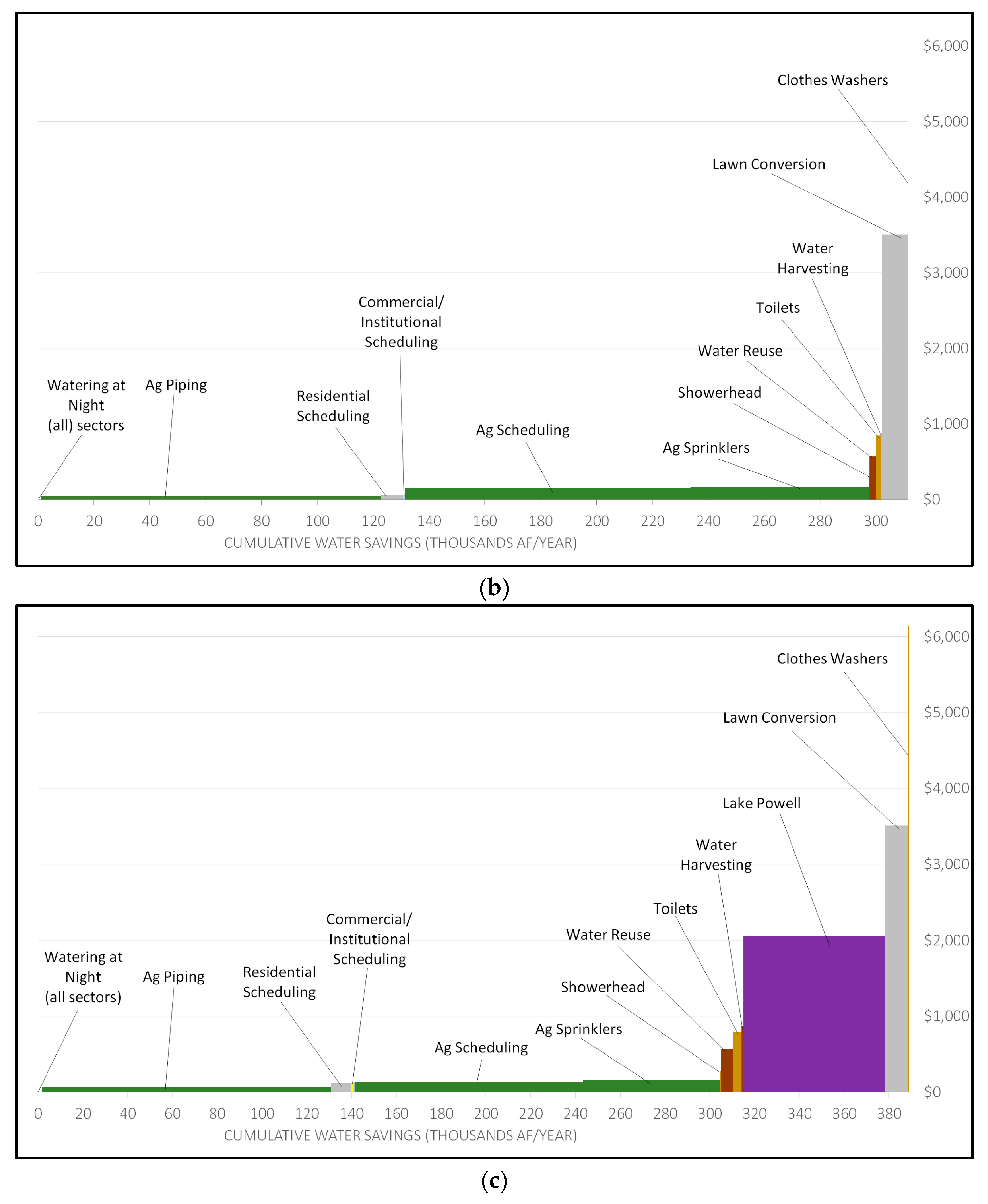
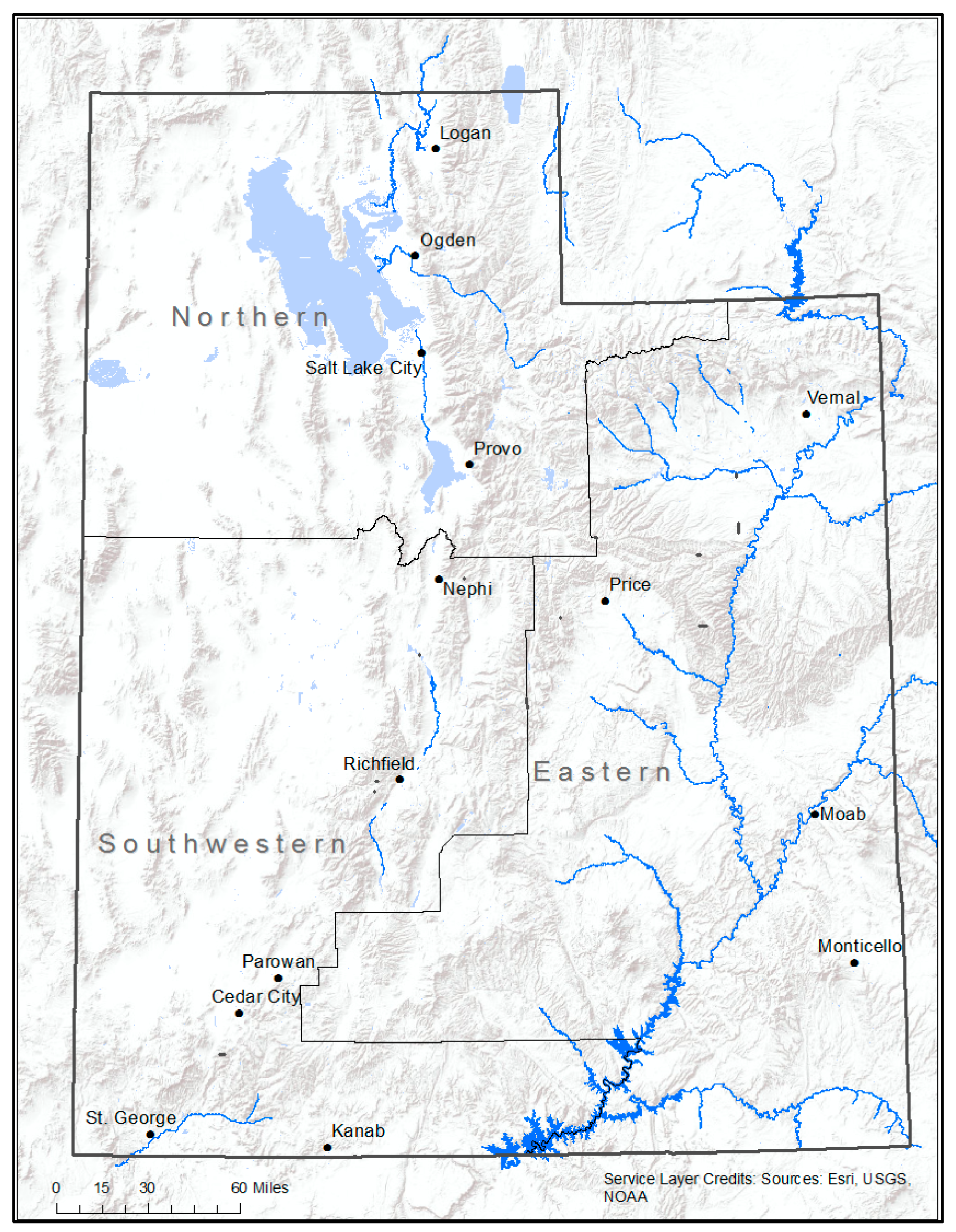
One potential use of a water efficiency supply curve is for policy makers and the public to examine the full range of options for providing water to growing urban areas. All the counties in the table except Washington are located in northern Utah. By 2060, these northern counties are projected to see population increases totaling 2,241,230 [
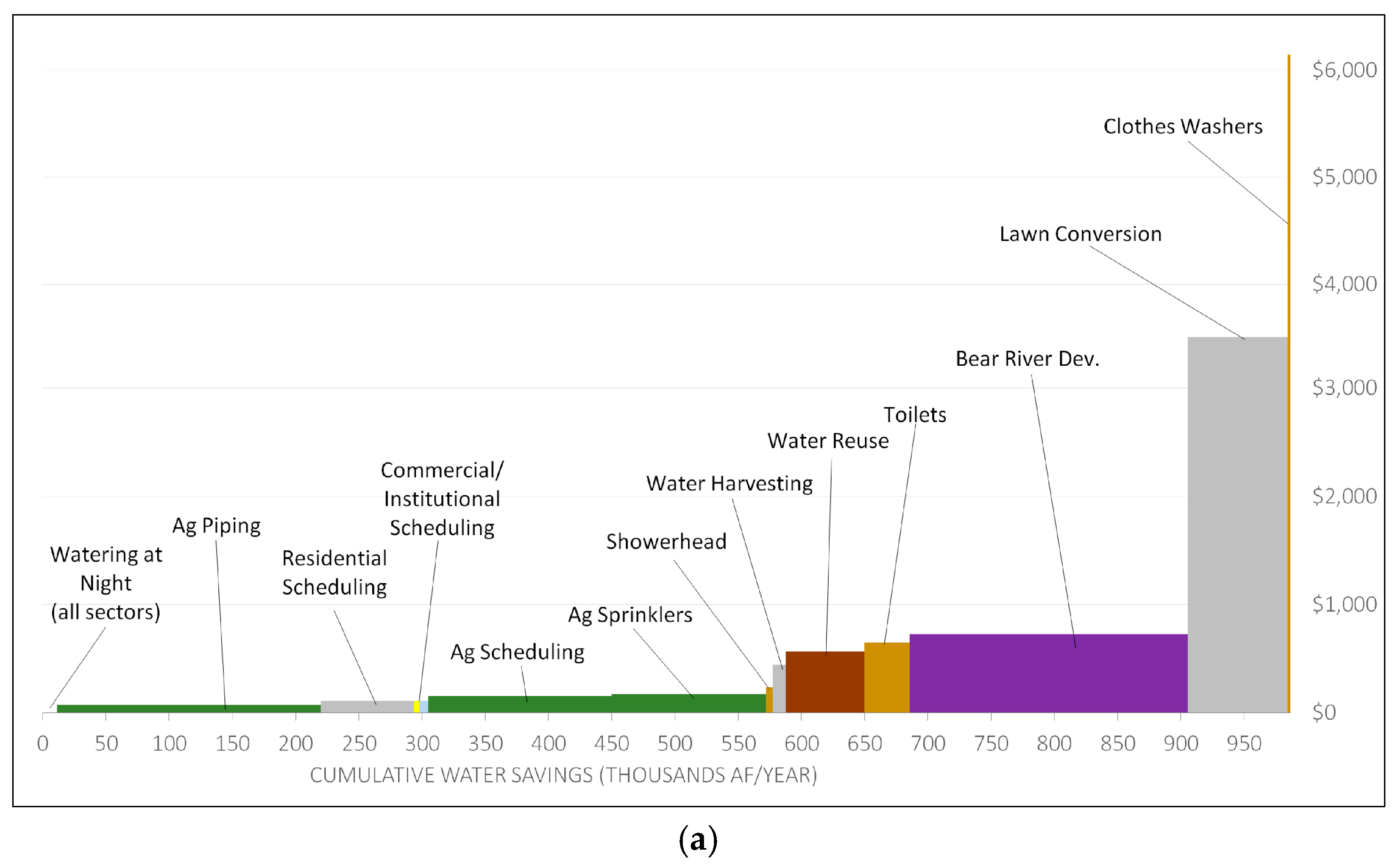
40]. This increase will require 564,213 additional AF of water at current per capita use rates. Using the cost curve for northern Utah, Figure 4a, the upper bound estimate of required urban supply could be met by undertaking only water conservation measures up to installing agricultural sprinklers. This water could be made available at or below a cost of $171 per AF, less than what most urban water users in these counties are currently paying, and substantially less than the per-AF cost of the Bear River Development Project.
Yet there are barriers to the use of water conservation savings to meet growing demand. In the short term, some of the potential water efficiency projects may not be feasible. For instance, a ditch-lining project would not address intra-year urban water shortfalls. This suggests the efficiency cost curve would be most useful in a long-term planning process, which would also enable planning for issues surrounding the potential environmental impact of the conservation measures. If efficiency savings are transferred out-of-basin, return flows and overall environmental water availability could decrease. This would be the case in northern Utah, where the highest water-use counties are not in the same basin as the highest demand-growth counties. A potential solution would be to introduce rules that limit transfer volumes to prior consumptive use [48].
Development projects such as dam and pipeline construction also have large environmental impacts that are not fully accounted for in the efficiency cost curves. Where possible, we include environmental mitigation costs. For instance, the Bear River Project would require substantial wetland mitigation, and this cost was included in the per AF cost estimates. However, other impacts are not included, for instance the effect of additional water diversions on the level of the Great Salt Lake, which in turn degrades ecosystems and can result in dust storms and other environmental problems [49].
Planning for how conservation savings can be moved to high-demand sectors is also an important aspect of using the efficiency curve. In some cases, new transportation infrastructure may be required, and construction and energy costs should be added to the per acre foot estimates when relevant. By examining the efficiency curves of more confined geographic regions, the impact of transportation costs will be reduced. Even when these costs are relatively low, rules against waste and third-party damages in most western states may limit the ability of right holders to transfer conserved water [50]. Farmers may fear partial forfeiture of their water right if conserved water cannot be put to immediate beneficial use on their farm [51]. Furthermore, their ability to transfer the water to a different sector may be opposed by other irrigators or environmental advocates [2]. Regulations locking water into agriculture can significantly depress water right value [52], making investments in even low-cost conservation projects uneconomical. Alternatives like development projects have high relative costs, but may be partially or fully publicly funded, delivering benefits to key interest groups [53,54]. Although the efficiency curve suggests water savings at low prices in agriculture, calls for farmers to increase efficiency without a mechanism to pay for conservation investments are unlikely to be successful. Economists have argued that the ability to transfer water makes each user account for the opportunity cost of its use—a necessary, although not sufficient, condition for improving water allocations [55].
Individual perceptions and behavior can also limit the adoption of water conservation. A nationwide study into individual perception of water use indicated that, on average, Americans underestimate the water use of common activities by a factor of two [56]. The same study found that when asked about ways to conserve water, people incorrectly considered behavioral changes to be more important to water conservation than upgrades. Another concern surrounds consumer acceptance of HE fixtures [57]. Though HE appliances have been around for over a decade and have benefited from continued innovation and national standards, there may be some lingering concerns over the effectiveness and durability of the fixtures. A 1999 survey of 1300 Ultra Low-Flush (ULF) toilet buyers in California concluded that “overall most consumers prefer their new ULF toilets to their old toilets [58],” while data on showerheads show a slight negative correlation between flow rate and customer satisfaction [59]. Other conservation areas are also affected by preferences and knowledge. Water reuse requires consumer buy-in, and there are potential obstacles in terms of environmental and human safety, and especially the social perceptions about the cleanliness of reused water [24]. Finally, the lack of knowledge about irrigation scheduling is likely a key barrier to its greater adoption [60].
The presence of barriers to effective implementation of the conservation measures discussed in this paper indicate that the efficiency curve is likely to be most beneficial as a tool in identifying conservation opportunities as part of a long-term planning process. This would provide time to overcome political, environmental, and educational barriers to conservation and provide adequate time for implementation of projects requiring longer leads.

5. Conclusions

Water conservation offers the potential to increase the supply of water in Utah at a relatively low cost. Agriculture and urban irrigation are the largest water users in the state of Utah and offer the largest potential to conserve water at relatively low prices. The water efficiency supply curve seeks to visually demonstrate what low-cost options exist and compare them across sectors. To meet demand through conservation, water conserved in high use sectors such as agriculture must be made available to high-demand sectors. Although there are barriers to the creation of mechanisms where entities with unmet demand can pay for conservation, doing so could create “win-win” outcomes where conservers and those paying for the water both benefit. The efficiency supply curve suggests that doing so could allow Utah to meet future water demands at low prices and in a way that is beneficial to all water users.

Supplementary Materials

The following are available online at www.mdpi.com/2073-4441/9/3/214/s1: spreadsheet of the data used in the paper and calculations.

Acknowledgments

We would like to thank Austin Brown, Kaaren Hodgson, Jack Trice, and Philip Visser for their contributions as research assistants, as well as Sara Sutherland, Niel Allen, Kelly Kopp, and four anonymous reviewers for their helpful comments. Funding was provided by iUTAH, NSF Award 1208732, a Utah State University Office of Research and Graduate Studies research catalyst grant, and UAES Project UTA01197.

Author Contributions

Eric Edwards conceived of and managed this research project and wrote the paper. Ryan Bosworth helped manage the data gathering and the writing of the paper. Patrick Adams, Viviane Baji, Amberlee Burrows, Coleman Gerdes, and Michelle Jones are listed in alphabetical order and contributed equally in providing the primary data for the project, creating the water efficiency supply curves, and writing the data section.

Conflicts of Interest

The authors declare no conflict of interest. Research sponsors had no role in the design of the study; in the collection, analyses, or interpretation of data; in the writing of the manuscript, and in the decision to publish the results.

References

  1. Chong, H.; Sunding, D. Water markets and trading. Annu. Rev. Environ. Resour. 2006, 31, 239–264. [Google Scholar] [CrossRef]
  2. Edwards, E.C.; Libecap, G.D. Water institutions and the law of one price. In Handbook on the Economics of Natural Resources; Halvorsen, R., Laytonm, D.F., Eds.; Edward Elgar Publishing: Northhampton, MA, USA, 2015; pp. 442–473. [Google Scholar]
  3. Brewer, J.; Glennon, R.; Ker, A.; Libecap, G. Presidential address water markets in the West: Prices, trading, and contractual forms. Econ. Inq. 2006, 46, 91–112. [Google Scholar] [CrossRef]
  4. Libecap, G.D. Institutional path dependence in climate adaptation: Coman’s “some unsettled problems of irrigation”. Am. Econ. Rev. 2011, 101, 64–80. [Google Scholar] [CrossRef]
  5. Grafton, R.Q.; Libecap, G.D.; Edwards, E.C.; O’Brien, R.B.; Landry, C. Comparative assessment of water markets: Insights from the Murray–Darling Basin of Australia and the Western USA. Water Policy 2012, 14, 175–193. [Google Scholar] [CrossRef]
  6. Office of Legislative Research and General Counsel (OLRGC). How Utah Water Works: An Overview of Sources, Uses, Funding, and Pricing. Utah Legislature Briefing Paper 2012. Available online: https://le.utah.gov/interim/2012/pdf/00002706.pdf (accessed on 26 February 2016).
  7. Granade, H.C.; Creyts, J.; Derkach, A.; Farese, P.; Nyguist, S.; Ostrowski, K. Unlocking Energy Efficiency in the U.S. Economy; McKinsey & Company: New York, NY, USA, 2009. [Google Scholar]
  8. Addams, L.; Boccaletti, G.; Kerlin, M.; Stuchtey, M. Charting Our Water Future: Economic Frameworks to Inform Decision-Making; 2030 Water Resources Group, McKinsey & Company: New York, NY, USA, 2009. [Google Scholar]
  9. Gleick, P.H.; Wolff, G.H.; Cushing, K.K. Waste Not, Want Not: The Potential for Urban Water Conservation in California; Pacific Institute for Studies in Development, Environment, and Security: Oakland, CA, USA, 2003. [Google Scholar]
  10. Ward, F.A.; Pulido-Velazquez, M. Water conservation in irrigation can increase water use. Proc. Natl. Acad. Sci. USA 2008, 105, 18215–18220. [Google Scholar] [CrossRef] [PubMed]
  11. Blum, A. Effective use of water (EUW) and not water-use efficiency (WUE) is the target of crop yield improvement under drought stress. Field Crops Res. 2009, 112, 119–123. [Google Scholar] [CrossRef]
  12. Seckler, D.; Molden, D.; Sakthivadivel, R. The concept of efficiency in water resources management and policy. In Water Productivity in Agriculture: Limits and Opportunities for Improvement; Seckler, D., Molden, D., Sakthivadivel, R., Eds.; Comprehensive Assessment of Water Management in Agriculture Series 2003; International Water Management Institute (IWMI): Colombo, Sri Lanka, 2003; pp. 37–51. [Google Scholar]
  13. Mohadjer, P. Residential Ultra-Low-Flush Toilet Replacement Program. Jordan Valley Water Conservancy District Report. West Jordan, UT, USA, 2003. Available online: http://www.cuwcc.org/Portals/0/Jordan%20Valley%20UFT%20Study%20030722.pdf (accessed on 3 April 2016).
  14. Mayer, P.W.; DeOreo, W.B.; Opitz, E.M.; Kiefer, J.C.; Davis, W.Y.; Dziegielewski, B.; Nelson, J.O. Residential End Uses of Water. American Water Works Association and AWWA Research Foundation Report. 1999. Available online: http://www.waterrf.org/PublicReportLibrary/RFR90781_1999_241A.pdf (accessed on 31 March 2016).
  15. DeOreo, W.B.; Mayer, P.; Dziegielewski, B.; Kiefer, J. Residential End Uses of Water, Version 2. Water Research Foundation, 2016. Available online: http://www.waterrf.org/4309 (accessed on 12 October 2016).
  16. Greene, B.; Mesner, N.; Brain, R. Rain Barrels in Utah; Utah State University Extension Sustainability Research Report; Utah State University: Logan, UT, USA, 2015; Available online: https://extension.usu.edu/waterquality/files-ou/Publications/Rainwater-Barrels-in-Utah-v-FINAL.pdf (accessed on 28 March 2016).
  17. American Community Survey (ACS). ACS 2010 (5-Year Estimates). U.S. Census Bureau Data. Available online: www.socialexplorer.com/tables/ACS2010_5yr/R11189913 (accessed on 27 May 2016).
  18. Utah Division of Water Resources (UDWR). State of Utah Municipal and Industrial Water Supply and Use Studies Summary 2010; Utah Department of Natural Resources Division of Water Resources Report; Utah Division of Water Resources (UDWR): Salt Lake City, USA, 2014.
  19. Endter-Wada, J.; Hall, A.; Jackson-Smith, D.; Flint, C. Utah’s Water Future: Perspectives on Water Issues in Utah’s Wasatch Range Metropolitan Area. Summary Report of Overall Findings from the iUTAH 2014 Household Survey, iUTAH Technical Report. 2015. Available online: http://data/iutahepscor.org/mdf/reports/SummaryReport-iUTAH2014HouseholdSurvey.pdf (accessed on 1 September 2016).
  20. Allen, N.; Utah State University Extension, Logan, UT, USA. Personal communication, 2016.
  21. Haley, M.B.; Dukes, M.D.; Miller, G.L. Residential irrigation water use in Central Florida. J. Irrig. Drain. Eng. 2007, 133, 427–434. [Google Scholar] [CrossRef]
  22. Sovocool, K.A. Xeriscape Conversion Study Final Report. Southern Nevada Water Authority Report. 2005. Available online: www.snwa.com/assets/pdf/about_reports_xeriscape.pdf (accessed on 27 March 2016).
  23. Environmental Protection Agency (EPA). Water Efficiency in the Commercial and Institutional Sector: Considerations for a WaterSense Program. Environmental Protection Agency Report; 2009. Available online: www3.epa.gov/watersense/docs/ci_whitepaper.pdf (accessed on 3 April 2016). [Google Scholar]
  24. Stonely, T.; Short, K.; Suflita, M.; Barrus, R.; Williams, J.; Smith, G. Water Reuse in Utah. State of Utah Natural Resources, Division of Water Resources Report. 2005. Available online: http://slco.org/WorkArea/DownloadAsset.aspx?id=2147520604 (accessed on 5 April 2016).
  25. Li, Y. Analysis of Urban Water Use and Urban Consumptive Water Use in Nebraska-Case Study in the City of Lincoln, Grand Island and Sidney. Master’s Thesis, University of Nebraska-Lincoln, Lincoln, NE, USA, 2013. [Google Scholar]
  26. Crook, J. Innovative Applications in Water Reuse and Desalination. Water Reuse Association Report. 2007. Available online: watereuse.org/wp-content/uploads/2015/10/WRA-103.pdf (accessed on 9 April 2016).
  27. United States Agricultural Census. State Summary Highlights. Volume 1, Chapter 2; 2012. Available online: www.agcensus.usda.gov/Publications/2012/Full_Report/Volume_1,_Chapter_2_US_State_Level/st99_2_001_001.pdf (accessed on 31 March 2016). [Google Scholar]
  28. United States Geological Survey (USGS). Water Use Data [Online Dataset]. 2012. Available online: waterdata.usgs.gov/ut/nwis/water_use (accessed on 1 August 2016). [Google Scholar]
  29. Burt, C.M.; Clemmens, A.J.; Bliesner, R.; Merriam, J.L.; Hardy, L. Selection of Irrigation Methods for Agriculture; American Society of Civil Engineers: Reston, VA, USA, 2000. [Google Scholar]
  30. Wamsley, N.; Store manager, Valley Implement, Logan, UT, USA. Personal communication, 2016.
  31. Scherer, T. Planning to Irrigate: A Checklist; North Dakota State University Extension Service Report: Fargo, ND, USA, 2013. Available online: www.ag.ndsu.edu/publications/crops/planning-to-irrigate-a-checklist (accessed on 15 March 2016).
  32. Tyson, T.W.; Curtis, L.M. 60 Acre Pivot Irrigation Cost Analysis; Biosystems Engineering Series Timely Information Report BSEN-IRR-08-01; Department of Biosystems Engineering, Auburn University: Auburn, AL, USA, 2008. Available online: www.aces.edu/timelyinfo/BioSysEng/2008/October/BSEN-IRR-08-01.pdf (accessed on 20 December 2016).
  33. Department of Water Resources (DWR). Fifteen Years of Growth and a Promising Future: The California Irrigation Management Information System. State of California, The Resources Agency, Department of Water Resources Report 1997. Available online: infohouse.p2ric.org/ref/32/31571.pdf (accessed on 20 December 2016).
  34. Cooley, H.; Christian-Smith, J.; Gleick, P.H. Sustaining California Agriculture in an Uncertain Future. Pacific Institute Report. Oakland, CA, USA, 2009. Available online: pacinst.org/app/uploads/2014/04/sustaining-california-agriculture-pacinst-full-report.pdf (accessed on 7 September 2016).
  35. Kranz, W.L.; Eisenhauer, D.E.; Retka, M.T. Water and energy conservation using irrigation scheduling with center-pivot irrigation systems. Agric. Water Manag. 1992, 22, 325–334. [Google Scholar] [CrossRef]
  36. Bureau of Reclamation (BOR). Selected Applications—WaterSMART Water and Energy Efficiency Grants [Online Database]. 2016. Available online: watersmartapp.usbr.gov/WaterSmart/ListProposals (accessed on 6 July 2016). [Google Scholar]
  37. Utah Division of Water Rights (UDWRi). Canal Companies and Contact Information [Online Data]. 2016. Available online: www.waterrights.utah.gov/canalinfo/canal_owners.asp (accessed on 6 July 2016). [Google Scholar]
  38. Bowen, Collins & Associates. Bear River Pipeline Concept Report Final. Report Prepared for the Utah Division of Water Resources, Consultant Job No. 233-09-01. 2014. Available online: www.cachecounty.org/water/br.html (accessed on 20 March 2016).
  39. Utah Board of Water Resources (UBWR). Lake Powell Pipeline: Final Study Report Number 20160502-5386; Final Socioeconomics and Water Resource Economics Study Report; Utah Board of Water Resources (UBWR): Salt Lake City, USA, 2016.
  40. Utah Governor’s Office of Management and Budget. 2012 Baseline City Population Projections [Online Data]. 2012. Available online: https://jobs.utah.gov/housing/owhlf/documents/GOPB2012BaselineProjections.pdf (accessed on 10 October 2016). [Google Scholar]
  41. City of Orem. New Tiered Water Rates. Available online: http://www.orem.org/new-tiered-water-rates/ (accessed on 6 October 2016).
  42. Salt Lake City. Water Rates: July 2016. Available online: http://www.slcdocs.com/utilities/PDF%20Files/UtilityRates/WaterrateswebCurrent.pdf (accessed on 6 October 2016).
  43. Ogden City. Rates and Discounts. Available online: http://www.ogdenwater.com/utilities-customer-service/rates-and-discounts/ (accessed on 6 October 2016).
  44. City of St. George. Utility Rates. Available online: https://www.sgcity.org/utilities/utilityrates (accessed on 6 October 2016).
  45. City of Logan. Resolution 12-36. Available online: http://www.loganutah.org/document_center/Public%20Works/1.12-36%20New%20Water%20Rates.pdf (accessed on 6 October 2016).
  46. Layton City. Welcome to Layton City. Available online: https://www.laytoncity.org/Downloads/finance/NewResidentInfoPacket.pdf (accessed on 6 October 2016).
  47. Maupin, M.A.; Kenny, J.F.; Hutson, S.S.; Lovelace, J.K.; Barber, N.L.; Linsey, K.S. Estimated Use of Water in the United States in 2010; US Geological Survey Report 2014, No. 1405; US Geological Survey: Reston, VA, USA, 2014.
  48. Johnson, R.N.; Gisser, M.; Werner, M. The definition of a surface water right and transferability. J. Law Econ. 1981, 24, 273–288. [Google Scholar] [CrossRef]
  49. Wurtsbaugh, W.; Miller, C.; Null, S.; Wilcock, P.; Hahnenberger, M.; Howe, F. Impacts of water development on Great Salt Lake and the Wasatch front. Watershed Sciences Faculty Publications 2016, Paper 875. Available online: digitalcommons.usu.edu/wats_facpub/875 (accessed on 1 October 2016).
  50. Ward, F.A.; King, J.P. Reducing institutional barriers to water conservation. Water Policy 1998, 1, 411–420. [Google Scholar] [CrossRef]
  51. Neuman, J.C. Beneficial use, waste, and forfeiture: The inefficient search for efficiency in western water use. Environ. Law 1998, 28, 919–1169. [Google Scholar]
  52. Edwards, E.C.; Cristi, O.; Edwards, G.; Libecap, G.D. An Illiquid Market in the Desert: The Role of Interest Groups in Shaping Environmental Regulation; National Bureau of Economic Research Working Papers, No. w21869; National Bureau of Economic Research: Cambridge, MA, USA, 2016. [Google Scholar]
  53. Reisner, M. Cadillac Desert: The American West and Its Disappearing Water; Penguin: New York, NY, USA, 1993. [Google Scholar]
  54. Shapiro, D.L. Can public investment have a positive rate of return? J. Polit. Econ. 1973, 81, 401–413. [Google Scholar] [CrossRef]
  55. Griffin, R.C. Water Resource Economics: The Analysis of Scarcity, Policies, and Projects, 2nd ed.; The MIT Press: Cambridge, MA, USA, 2016. [Google Scholar]
  56. Attari, S.Z. Perceptions of water use. Proc. Natl. Acad. Sci. USA 2014, 111, 5129–5134. [Google Scholar] [CrossRef] [PubMed]
  57. Chesnutt, T.W.; Pekelney, D.M. Urban Water Conservation Implementation Challenges and Opportunities. California Urban Water Agencies Report. Encinitas, California, USA, 2004. Available online: www.cuwa.org/pubs/092304WaterConsImplementationChallenges.pdf (accessed on 6 October 2016).
  58. The Metropolitan Water District of Southern California (MET). Ultra-Low Flush Toilet Program 1999 Residential Customer Satisfaction Survey. 1999. Available online: www.allianceforwaterefficiency.org/WorkArea/DownloadAsset.aspx?id=850 (accessed on 31 March 2016).
  59. California Utilities Statewide Codes and Standards Team (CUSCST). Multi-Head Showers and Lower-Flow Shower Heads: 2013 California Building Energy Efficiency Standards. California Statewide Utility Codes and Standards Program Report. Available online: www.map-testing.com/assets/reports/CA_Statewide%20CodesStandards_2013_CASE_R_Shower_Heads_Sept_2011.pdf (accessed on 31 March 2016).
  60. Kopp, K.; Utah State University Extension, Logan, UT, USA. Personal communication, 2016.
Figure 1. Map of the Utah geographic regions used for this paper.
Water 09 00214 g001
Figure 2. Agricultural water savings in Utah counties: (a) total water savings; (b) per-acre water savings.
Water 09 00214 g002
Figure 3. Water efficiency supply curves for Utah.
Water 09 00214 g003
Figure 4. Water efficiency supply curves for Utah’s regions: (a) northern Utah; (b) eastern Utah; (c) southwestern Utah.
Water 09 00214 g004aWater 09 00214 g004b
Table 1. Conservation measures by category.
CategoryConservation Measures
Residential IndoorLow-flow toilets
Low-flow showers
High-efficiency clothes washers
Residential OutdoorRainwater harvesting
Watering at night
Irrigation scheduling
Partial turf conversion
CommercialLandscape watering at night
Landscape irrigation scheduling
WastewaterSecondary wastewater irrigation
AgricultureConversion to sprinkler irrigation
Improved irrigation efficiency
Canal piping
DevelopmentBear River Development
Lake Powell Pipeline
Table 2. Indoor Residential Conservation.
Type of ReplacementNumber ReplacedAcre-Feet (AF) ConservedAverage Cost per Acre-Foot (AF)
Toilets1,361,98441,667$673
Showers371,4245693$241
Washing Machines375,4244804$6145
Table 3. Outdoor Residential Conservation.
Conservation MeasureAF ConservedAverage Cost per AF
Rainwater Harvesting11,886$482
Watering at Night12,666$0
Seasonal Scheduling90,335$109
Turf Conversion104,708$3508
Table 4. Development project present value costs.
ProjectAnnual AFCapital CostMaintenanceNet PowerEnviron. MitigationCost per AF
Lake Powell (Low)62,996$1163 M$93 M$37 M$75 M$1414
Lake Powell (High)62,996$1798 M$143 M$108 M$560 M$2697
Bear River B220,000$1682 M$133 M$97 M$801 M$803
Bear River M220,000$1823 M$144 M$97 M$117 M$646
Table 5. Regional and statewide savings (in AF) and cost estimates.
EasternNorthernSouthwesternUtah
TechnologyCostSavingsCostSavingsCostSavingsCostSavings
Resident. night$01123$010,278$01266$012,666
Commer. night$022$0451$052$0525
Instit. night$035$0725$083$0844
Ag piping$44121,474$74208,478$70129,474$58459,425
Resident. schedule$658007$11273,301$1269028$10990,335
Commer. schedule$65215$1124392$126505$1115112
Instit. schedule$65345$1127054$126811$1118211
Ag schedule$156102,283$158145,011$142102,056$153349,351
Ag sprinklers$16864,013$171122,070$16061,130$167247,213
Showers$303239$2334891$283562$2415693
Rain barrels$879345$44210,777$870764$48211,886
Water reuse$5682158$56861,972$5685042$56869,173
Toilets$8471751$65135,798$7894116$67341,667
Bear River $724220,000 $724220,000
Lake Powell $205562,996$205562,996
Turf conversion$35089281$350884,963$350810,464$3508104,708
Washers$6145254$61453993$6145557$61454804
Total 311,545 994,153 388,908 1,694,608
Table 6. Projected population and water demand.
County (Water Rate City)Water Use (AF per Person)Urban Rate per AFPopulation 2010Population 2060Added Demand 2060 1 (AF)
Utah (Orem)0.24$296516,5641,398,074215,343
Salt Lake (Salt Lake City)0.24$4341,029,6551,812,891187,964
Weber (Ogden)0.29$638231,236449,05362,331
Cache (Logan)0.29$378112,656273,81746,798
Davis (Layton)0.26$98306,479503,98551,778
Washington (St. George)0.37$67138,115581,731164,307
Note: 1 At current per-person water use rate.

