Article

Modeling Potential Impacts of Climate Change on Streamflow Using Projections of the 5th Assessment Report for the Bernam River Basin, Malaysia

by
Nkululeko Simeon Dlamini
1,
Md Rowshon Kamal
1,*,
Mohd Amin Bin Mohd Soom
2,
Mohd Syazwan Faisal bin Mohd
3,
Ahmad Fikri Bin Abdullah
1 and
Lai Sai Hin
4
1
Department of Biological and Agricultural Engineering, Faculty of Engineering, Universiti Putra Malaysia, 43400 UPM Serdang, Selangor, Malaysia
2
Faculty of Sustainable Agriculture, Universiti Malaysia Sabah (UMS), Jalan UMS, 88400 Kota Kinabalu, Sabah, Malaysia
3
Water Resources Research Centre and Climate Change, NAHRIM, 43300 Seri Kembangan, Selangor, Malaysia
4
Department of Civil Engineering, Faculty of Engineering, University of Malaya, 50603 Kuala Lumpur, Wilayah Persekutuan Kuala Lumpur, Malaysia
*
Author to whom correspondence should be addressed.
Water 2017, 9(3), 226; https://doi.org/10.3390/w9030226
Submission received: 17 January 2017 / Revised: 7 March 2017 / Accepted: 15 March 2017 / Published: 20 March 2017
(This article belongs to the Special Issue Adaptation Strategies to Climate Change Impacts on Water Resources)

Abstract

:
Potential impacts of climate change on the streamflow of the Bernam River Basin in Malaysia are assessed using ten Global Climate Models (GCMs) under three Representative Concentration Pathways (RCP4.5, RCP6.0 and RCP8.5). A graphical user interface was developed that integrates all of the common procedures of assessing climate change impacts, to generate high resolution climate variables (e.g., rainfall, temperature, etc.) at the local scale from large-scale climate models. These are linked in one executable module to generate future climate sequences that can be used as inputs to various models, including hydrological and crop models. The generated outputs were used as inputs to the SWAT hydrological model to simulate the hydrological processes. The evaluation results indicated that the model performed well for the watershed with a monthly R2, Nash–Sutcliffe Efficiency (NSE) and Percent Bias (PBIAS) values of 0.67, 0.62 and −9.4 and 0.62, 0.61 and −4.2 for the calibration and validation periods, respectively. The multi-model projections show an increase in future temperature (tmax and tmin) in all respective scenarios, up to an average of 2.5 °C for under the worst-case scenario (RC8.5). Rainfall is also predicted to change with clear variations between the dry and wet season. Streamflow projections also followed rainfall pattern to a great extent with a distinct change between the dry and wet season possibly due to the increase in evapotranspiration in the watershed. In principle, the interface can be customized for the application to other watersheds by incorporating GCMs’ baseline data and their corresponding future data for those particular stations in the new watershed. Methodological limitations of the study are also discussed.

1. Introduction

The Intergovernmental Panel on Climate Change (IPCC) and other researchers have reported compelling concerns revolving around the impact of climate change on our societies [1,2,3]. Climate change is a global phenomenon exhibited by three prominent signals, that is: (1) global average temperatures are gradually increasing; (2) changes in global rainfall patterns; and (3) rising of sea levels. One of the major impacts of this phenomenon is on local water resource availability, whose impact will be felt by many sectors, including agriculture. According to the recent Fifth Assessment Report by IPCC, the increase in temperature and warm trends will continue across most of the Southeast Asia region in the current century and that water is expected to be a major challenge because of the corresponding demand for it and lack of adaptive capacity to the impacts [4]. In Malaysia, climate change-related policies are still underway, and most of the climate knowledge is largely inferred from the Southeast Asia region due to limited local studies [5,6]. Effective adaptation measures require good understanding of local changes taking into account the projections provided by global climate models. Nowadays, basin-wide hydrologic investigations are becoming a basis for the implementation of robust adaptation strategies [7,
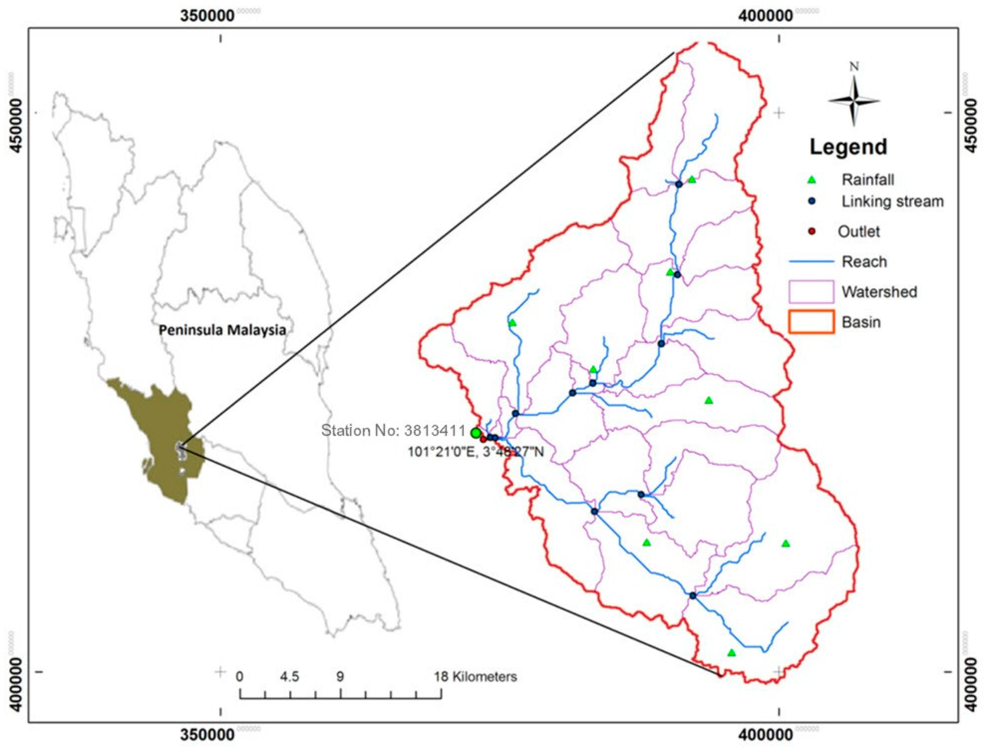
8]. This contribution assesses the effects of climate change on the hydrological flows of the Upper Bernam River Basin in Malaysia.
Rice is an important staple food for a large section of the people, and yet, its water demand is relatively high, accounting for over 80% of the country’s water resources [9,10]. The country’s rice self-sufficiency policy of 85% is sustained through practicing the double-cropping method, which requires constant supply of paddy water in the command areas at all times. Most of the rice farming systems are run-of-the-river systems and depend largely on direct river flows. Due to insufficient flows in certain periods, cultivation of paddy is usually staggered in phases to ensure constant supply of water on rice fields. However, it is a well-known fact that in many run-of-the-river irrigation schemes, water demand seldom matches the unreliable streamflows of rivers. In the past, this has led to difficulties in allocating irrigation water to paddy farmers. The Bernam River Basin is one important basin that supports paddy irrigation. The future outlook of climate change may thus pose serious implications on water resources for future paddy production in this basin. A previous study assessed only the impact of future land use changes on the flow of this river [11]. Assessment that also accounts for climate change is therefore critical for planning and management of future water allocations.
To do this, information derived from Global Climate Models (GCMs) is currently the most suitable in assessing both past and future likely changes in climate scenarios [12]. This climate information is then used as input to drive hydrologic and water demand models. Long-term locally-observed climate data are also required to validate climate model outputs to capture local conditions. However, direct application of GCM outputs to any model for subsequent assessment of impact is discouraged in climate studies because of resolution issues. GCMs run their simulations on large scales to account for various grids across the globe. Yet, the hydrologic system or cropping system of interest is affected by local climatic conditions [2,13]. The Bernam River Basin, for instance, is covered within an area of 1.2° × 1.0° longitude and latitude, whereas a GCM typically takes about 2.8° × 2.8° longitude and latitude. To overcome this issue, downscaling is adopted, a process of bringing down the climate information from GCM to hydrologic scales to produce outputs of higher resolution, which are more realistic with the local scale before assessing the risks associated with the future hydrologic scenarios.
Several downscaling techniques have advanced over the past two decades, evolving from two major schemes; dynamic downscaling and statistical downscaling techniques. The dynamic technique is often viewed as a mini-GCM because it attempts to simulate local climate variables by reducing the horizontal area covered (typically around 25 by 25 km or even smaller) using the same boundary conditions as the driving GCM. Although they produce high resolution climate data, they have not been widely adopted because of the costs and complexities involved in running this type of technique [14] in order to capture local- or regional-scale climate variables. Statistical downscaling techniques, involving methods such as, weather typing procedures, transfer functions and stochastic weather generators, are the most popular methods used in climate change studies today [2,15]. They produce future climate scenarios based on a statistical relationship between climate variables at one or more GCM grid points with the variable of interest at a particular station. They are adopted because they are relatively inexpensive to apply and also give point climate data at a specific site of interest [16]. A more inclusive review of these approaches as relates to hydrologic impact assessment is covered by [7]. Each method has its merits and demerits, and the choice will depend largely on the purpose of the study, the availability of observed data, the scale of required data (daily or monthly, etc.) and the size of the study area. In areas where there are no readily-available regional climate model outputs, such as in Malaysia, the change factor or delta method is widely used [7] on the GCM outputs for hydrological and crop modeling studies [2,17,18,19].
Carbon emission scenarios are the main forcings in driving climate models. Scenarios are pictures or images of how the world is likely to evolve in the future in terms of greenhouse gas [20]. In the present study, we use the latest scenarios, called Representative Concentration Pathways (RCPs), which have rarely been applied in Malaysia. RCPs offer a better understanding in terms of the concentration of future greenhouse gases for running climate models than previous scenarios [21,22]. The downscaled simulation outputs are then applied in a separate hydrologic model to develop future hydrologic scenarios for a particular river basin. The Soil and Water Assessment Tool (SWAT) is a widely-applied model in assessing hydrologic impacts. Global SWAT model applications are summarized in the work of [23].
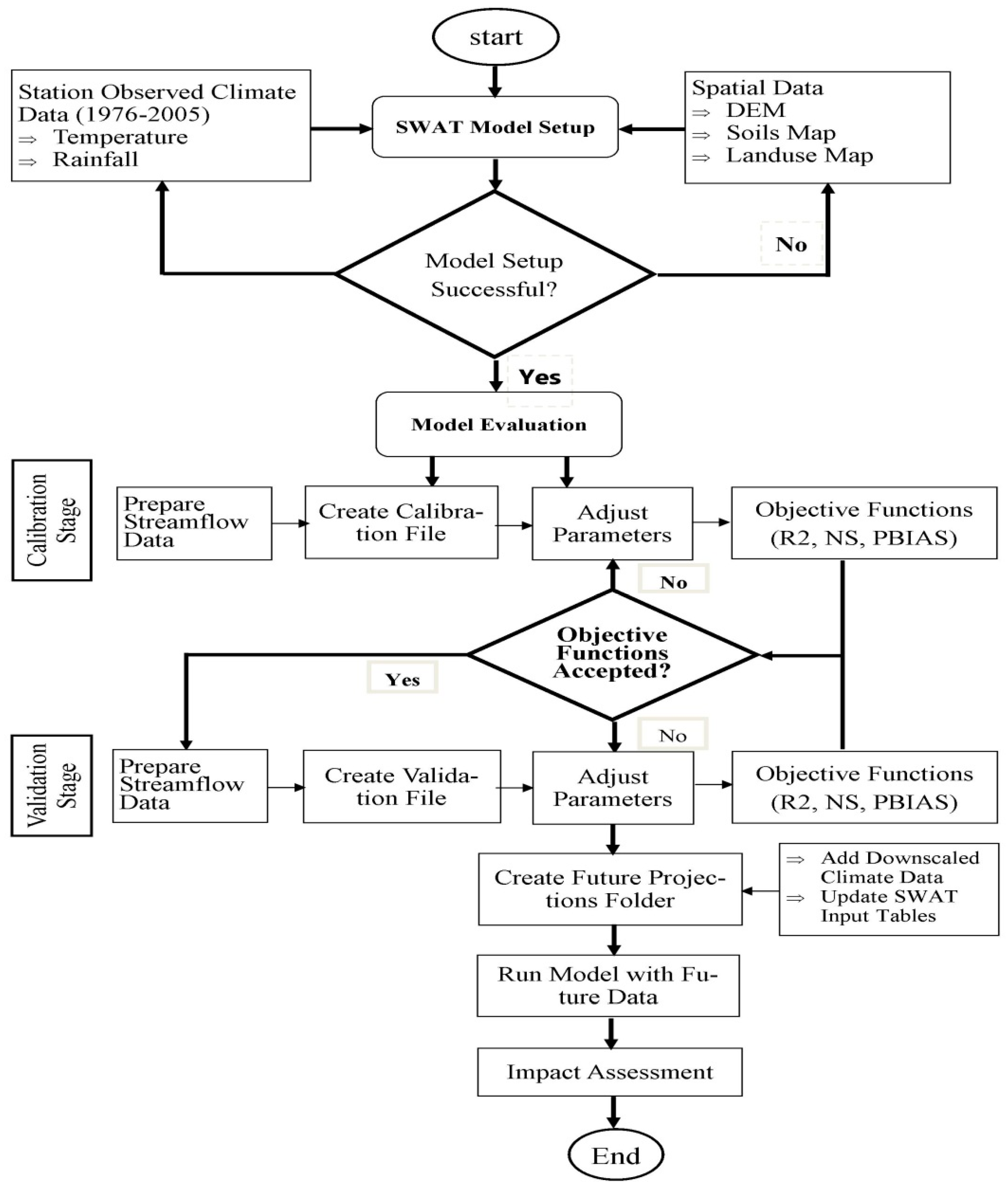
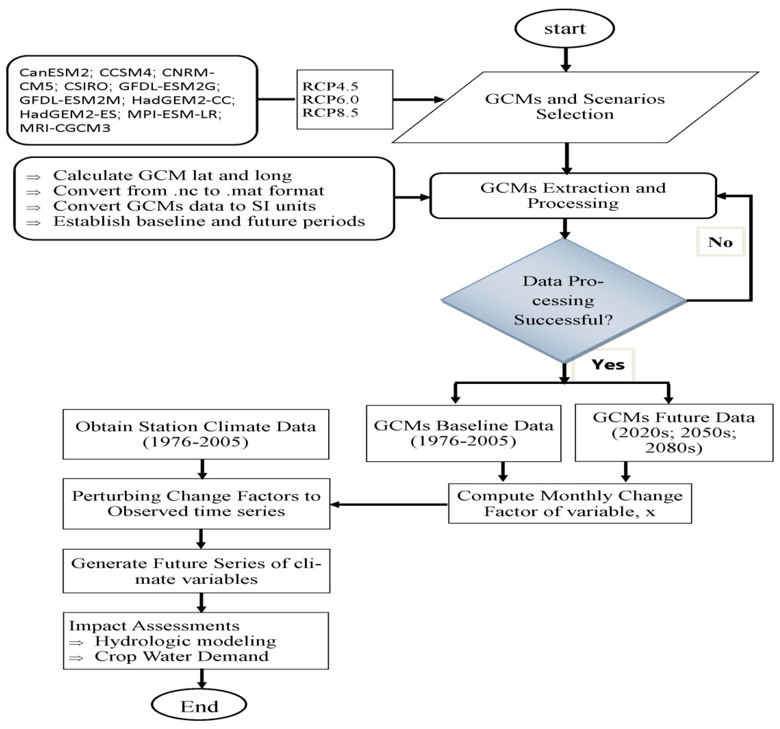
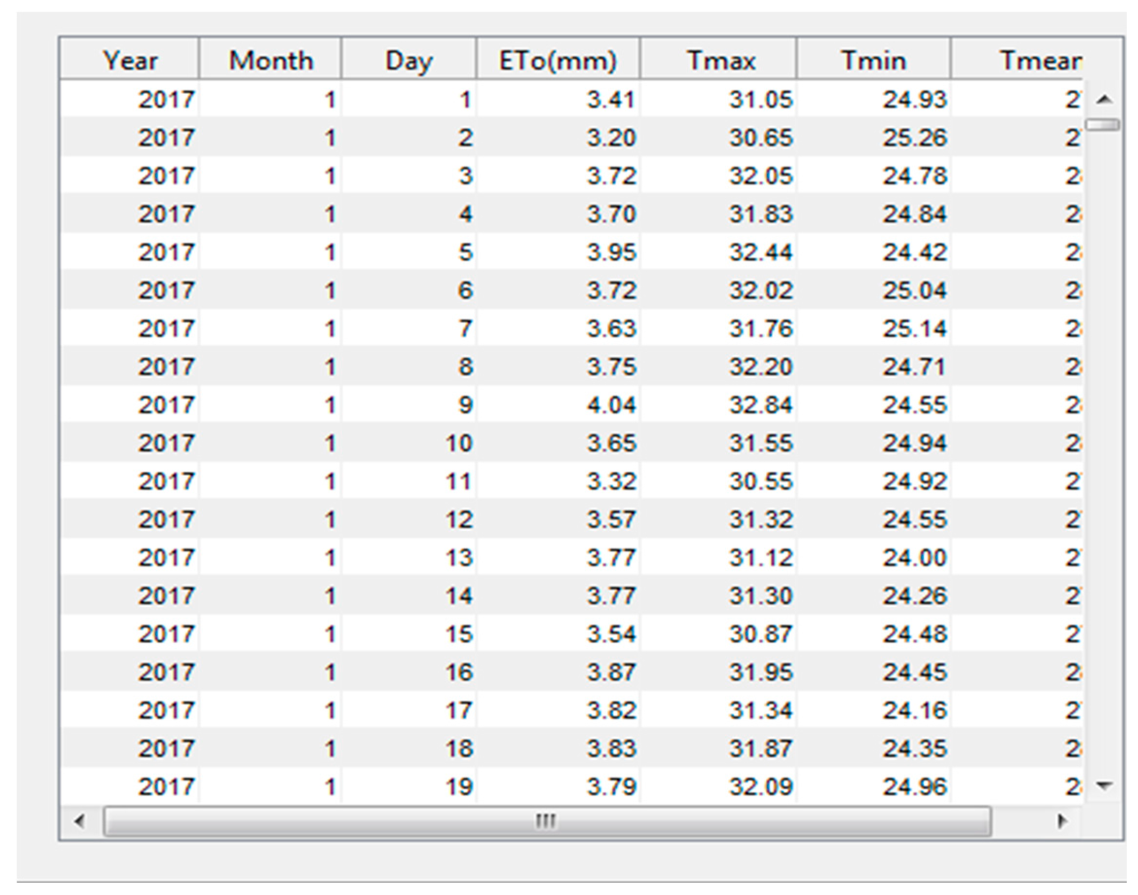
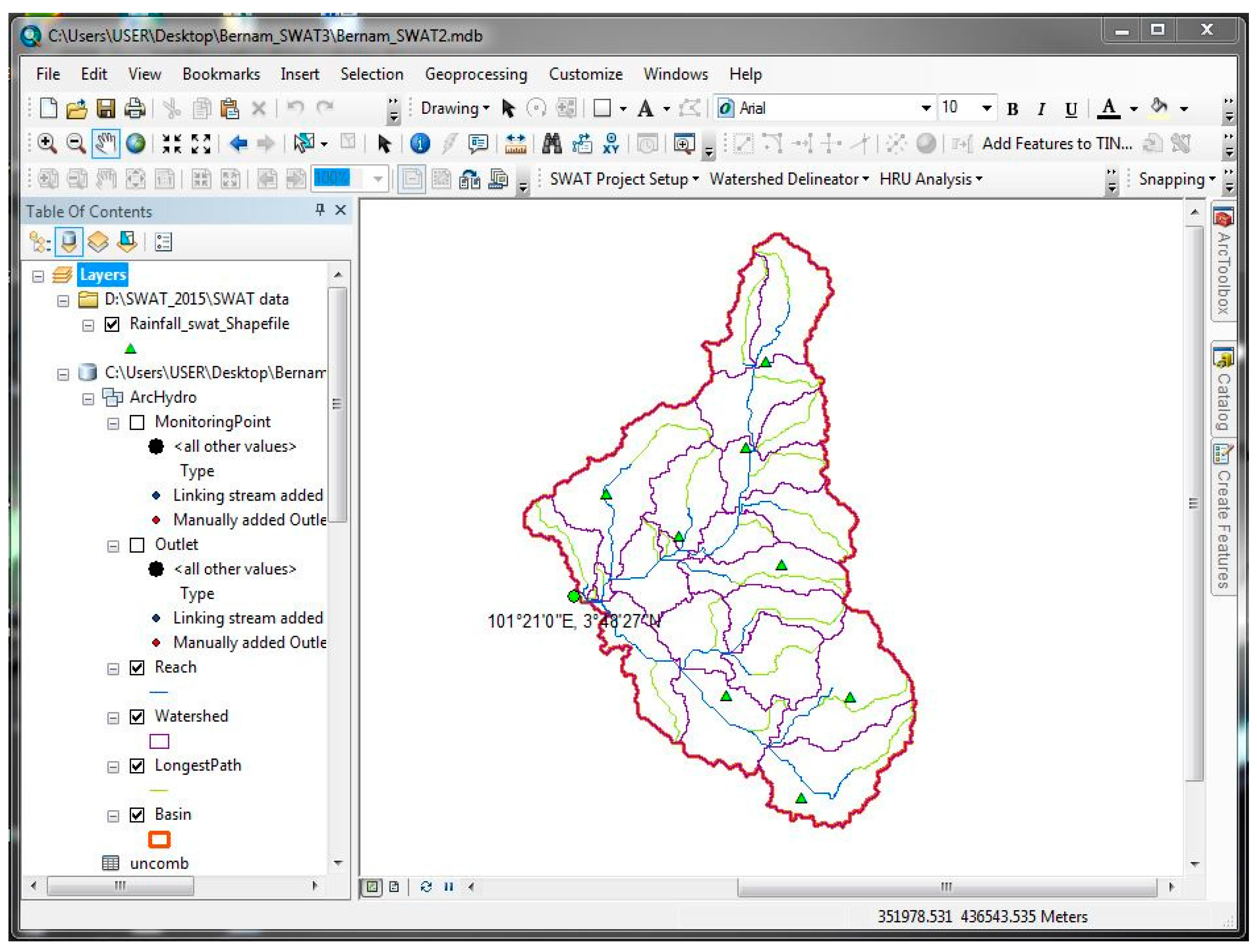
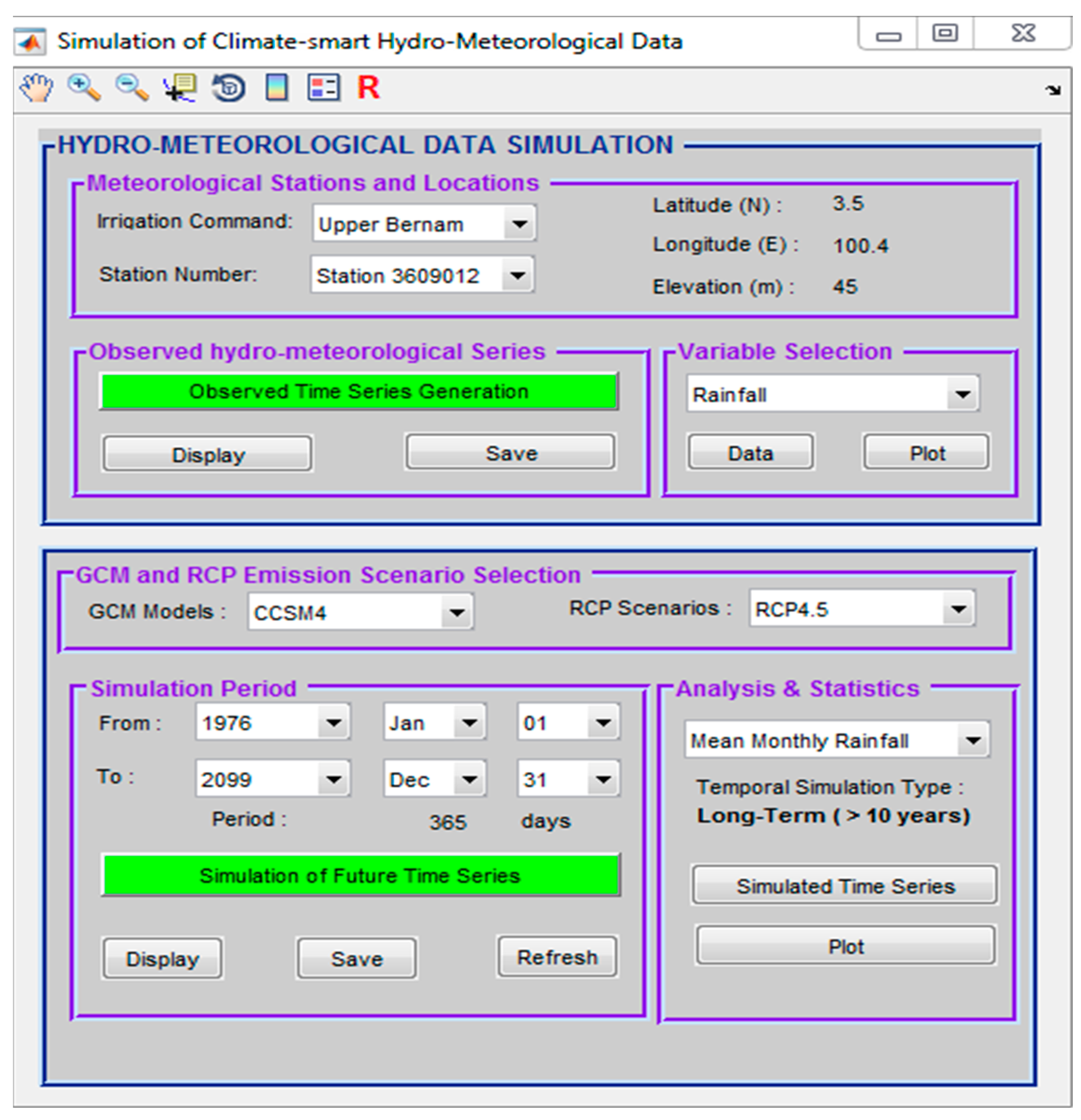
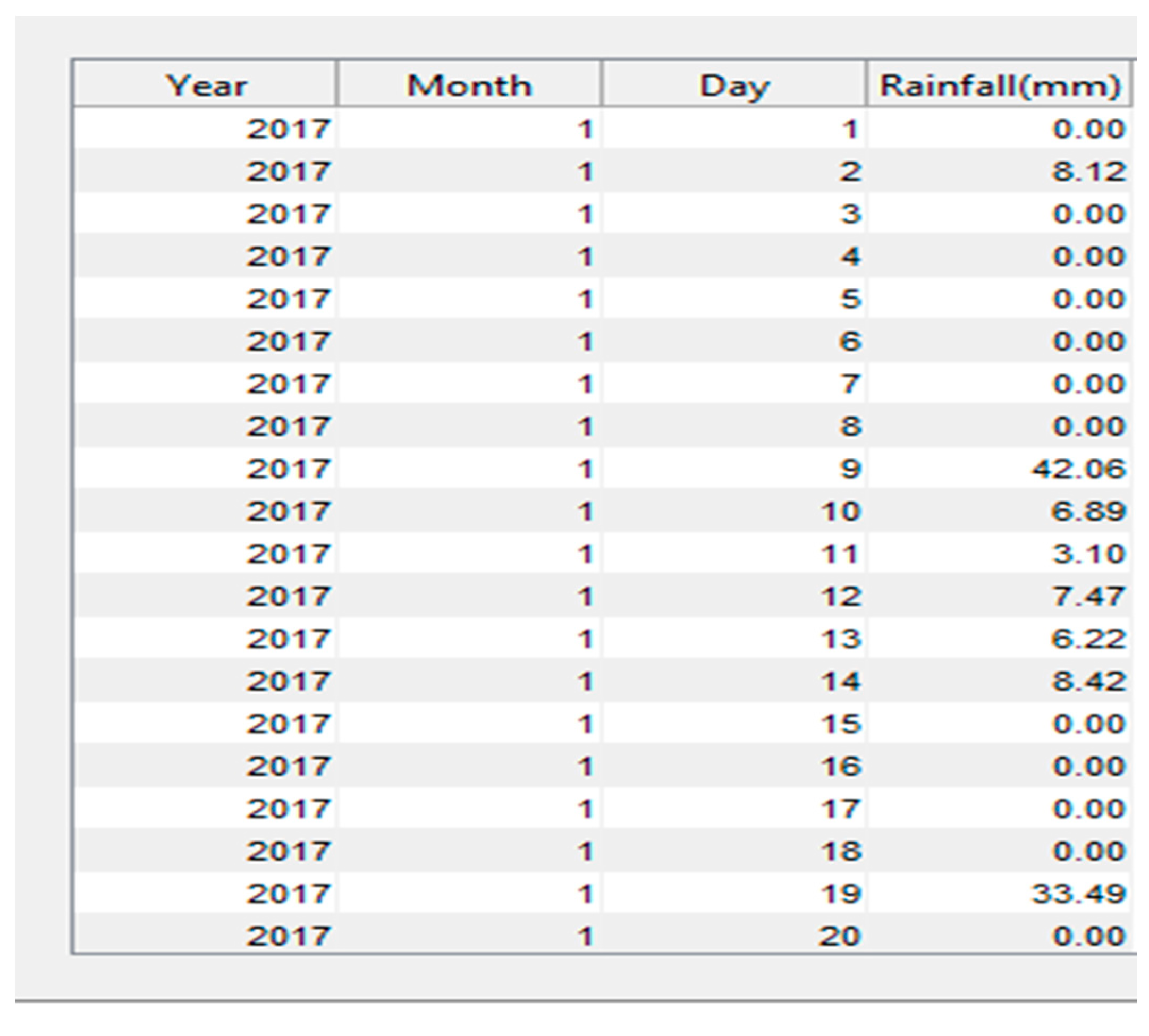
The main hydrologic impact of interest in this study is the monthly flows of the Bernam River Basin as a main source of water for the large irrigation scheme in the basin. However, generating future climate scenarios is still a challenge, as it involves several steps before outputs can be employed in impact assessments. In this study, a simple graphical user interface was developed that integrates all of the procedures of assessing climate change impacts, which includes GCMs and scenarios’ selection, downscaling procedures, climate projections. These procedures are linked in one executable module to generate future climate sequences that can be used as inputs to various models including hydrological and crop models. The core objective of the study, therefore, is to investigate the potential effects of climate change on the flows of the Bernam River Basin using the projections of the 5th Assessment Report of the IPCC. This involves: (1) evaluating the performance of the SWAT model for the simulation of flows in the Bernam River Basin; (2) developing an interface for the rapid simulation of climate variables (e.g., rainfall, temperature, etc.) at the local scale from large-scale climate models; (3) evaluating future changes in rainfall and temperature patterns in the basin; and (4) investigating future changes in the flow scenarios of the basin. The results will be used as input in a decision support system for modeling water allocation and planning for a run-of-the-river irrigation scheme under climate change impacts in Malaysia.

2. Materials and Methods

2.1. The Watershed

The Upper Bernam River watershed is located at the boundary between the States of Perak and Selangor (Figure 1). The river covers a basin area of 1097 km2 stretching about 127 km before discharging into the Malacca Strait. The watershed has a mean elevation of about 950 m above sea level (m a.s.l.). The lowest point is situated at 201 m a.s.l. at the Bernam River gauging station No. 3813411, and the highest point is 1800 m a.s.l. at the edge of Pahang State. The river flow routes through sections of a large forest complex, oil palm, rubber and paddy farms. The watershed has a humid tropic climate that is largely characterized by the two predominant rainfall seasons [24], the Southwest Monsoon and the Northeast Monsoon. In the agricultural context, these have generally been defined as the “dry season” (January–June) and the “wet season” (July–December), respectively. The average annual rainfall over the watershed is 2545 mm, which is concentrated mostly between September and December and to a limited extent in April–May. Generally, maximum and minimum temperatures are fairly constant throughout the year in Malaysia with the mean values of 31.5 °C and 22.3 °C, respectively [25].
Agriculture is the dominant type of land use within the basin with over 60% of the land being used for forest, oil palm, rubber and paddy rice production. The river is the major source of irrigation water for the Tanjung Karang Rice Irrigation Scheme (TAKRIS), located near the watershed. TAKRIS is the 4th largest rice scheme in the country with approximately 19,800 hectares planted with rice all year round under the double-cropping planting system. Because of low flows in the Bernam runoff during the dry season, rice cultivation has been re-staggered into four Irrigation Service Areas (ISAs I, II, III and IV) beginning from January (ISA I) through to June (ISA IV). The cycle is repeated for the wet season from July (ISA I) through to October (ISA IV) before the heavy rains begins. Water is diverted at the Bernam headworks, conveyed by canal systems and distributed in-field by several tertiary canals. Flow records at the SKC station have relatively long records dating as far back as the 1960s. The streamflow is high during the wet season and declines during the dry season, and reports on potential water shortages and rationing are common during the latter period. In the past, the rice scheme suffered frequent water shortages due to: (1) water shortages during the dry season months; (2) constraints to the delivery of water and timing; and (3) water management practices that led to inefficient use of water. Therefore, knowledge of future streamflow is indispensable for this scheme in order to minimize its proneness to likely future drought conditions.

2.2. The Study Framework

This study has combined three aspects: firstly, developing a MATLAB-based interface for rapid simulation of climate variables at the local scale from large-scale climate models; secondly, for input to a hydrological model, assessment of climate change impacts on the statistically downscaled climate variables (rainfall and temperature); and lastly, assessment of the response of the river’s hydrologic system to changes on downscaled climate variables. The methodological framework followed for the study is shown in Figure 2 and involves: (i) the preparation of spatial and climate data into SWAT format; (ii) model setup, including watershed delineation and Hydrologic Response Units (HRUs) definition; (iii) model calibration and validation; (iv) downscaling of climate variables; and (v) application into the hydrologic model.

2.3. Data Source

The SWAT model requires observed climate and spatial data to force the rainfall-runoff simulation process. Detailed information about the data used in this study, including the data type and their source, is presented in Table 1.
Observed climate data in the watershed area are largely of poor quality due to a series of years of missing values. For this reason, a gridded daily hydro-meteorological dataset developed in a separate study [26], covering the whole Peninsular Malaysia, was used in this study. The variables used include daily rainfall (mm/day) and daily air temperatures (°C) (maximum and minimum). The data are gridded from daily observed data at a spatial resolution of approximately 5 km based on Angular Distance Weighting (ADW) procedure, which performs relatively better in areas with sparse data, like in Malaysia. The gridded data were developed using observed data obtained from different sources, including the automatic data logger and the telemetry network database of the Department of Irrigation and Drainage (DID) and the Malaysia Meteorological Department (MMD). A small amount of data was also obtained from the publicly accessible Global Summary of the Day (GSOD) archive and the Global Energy and Water Balance Experiment (GEWEX) research program Asian Monsoon Experiment (GAME) archive. The data were checked for quality using several levels of data quality control, including discarding daily observations with statistics not supported by long-term MMD key stations and also station series with less than 40 rain days and more than 247 rain days, as well as annual amounts not consistent with long-term records. A detailed overview of the data processing, quality control and the methodology used in the data development is given by [26,27]. The final processed data used in this study were requested and obtained from the Department of Irrigation and Drainage (DID) of Malaysia. Eight existing stations of rainfall and two for temperature located within the watershed were considered to represent the historical spatial climate of the basin. The gridded data were extracted from the DID database based on the coordinates of these stations from January 1976 to December 2005. For rainfall, a threshold value of 0.5 mm was applied in order to remove small rainfall amounts.
Spatial information used in the model includes watershed land cover/land use, soils and the Digital Elevation Model (DEM). The DEM data corresponding to the study area were obtained from DIVA-GIS (www.diva-gis.org), DIVA-GIS is a free computer program for mapping and geographic data analysis (GIS). The DEM was re-sampled to 30-m resolution and used to apportion the basin into 23 sub-basins and 145 HRUs and generate drainage patterns based on the spatial data distribution within the watershed (Figure 3). The elevation in the Bernam River basin ranges from 201 m in the lower plains to 1800 m in the upper region.
Soil and land use maps of 2002 were obtained from the Department of Agriculture (DOA) as jpeg and were digitized into vector format using ArcGIS10.1. The land use map distinguishes eight land use classes, with forest (53.5%), oil palm (21.7%) and rubber (18.1%) being dominant in the study area. Soil properties such as soil depth, texture and water holding capacity were obtained from several sources for the SWAT database [28,29]. Details on land use and soil distribution are shown in Figure 4b,c.
Daily streamflow records (m3/s) at the Bernam River gauging station No. 3813411, located at the outlet of Sub-basin 16, were obtained from the same department (DID). The station has long enough flow records, but only the segment from January 1976 to December 2005, corresponding to the climate data, was used in the study. Missing values of discharge were filled using long-term averages of the station.
Future climate projections over the Upper Bernam watershed were extracted from ten Global Climate Models (GCMs) obtained from the Program for Climate Model Diagnosis and Inter-comparison (PCMDI) (http://pcmdi3.llnl.gov/esgcet/home.htm). GCMs were selected on the basis of: (1) the availability of the climate variables on a daily time scale for both baseline and future runs; and (2) addressing of inherent uncertainties in climate models. Three emission scenarios, namely the medium stabilization scenario (RCP4.5), the medium-high scenario (RCP6.0) and the very high scenario (RCP8.5), were selected on the basis of the high social development index exhibited by Malaysia based on a UNEP study [30]. However, at the time of downloading these data, the very-low forcing scenario (RCP2.6) was not available due to technical issues when changing from the old gateway to the new official site. Table 2 gives an overview of the GCMs used in this study.

2.4. The SWAT Model

The SWAT model, a product of the United States Department of Agriculture (USDA), is one of the hydrological models used by several researchers and agencies for water resource planning, which has contributed significantly in many scientific fields globally, including climate change assessments [18,31]. The extensive support from model developers through sufficient documentations on its use, annual seminars and continuous improvements by its users are some of the reasons that motivate its world-wide adoption, including this study. The model is a continuous-time, semi-distributed, process-based river basin model for simulation of the impact of land management practices and natural factors on water, sediment and nonpoint source pollution in large watersheds [32]. The key components for the SWAT model consist of; hydrology, weather, sedimentation, nutrients, crop growth, agricultural management and stream routing [33]. In this study, the focus is only on the hydrologic component of the model. SWAT offers spatial details of the watershed by way of dividing the watershed into several smaller units called sub-basins. The sub-basins are further divided into homogenous standardized units known as ‘Hydrologic Response Units’ (HRUs) characterized by uniform soil-land use and slope representing a unique hydrologic response [34]. Water balance is the main driving force behind the SWAT model, as it affects many of the processes, including plant growth and movement of sediments and other components. Soil water content is computed using the water balance equation (Equation (1)).
SW t = SW 0 + i = 1 t ( R day Q surf E a W seep Q gw )
where SWt denotes the soil water content (mm), SW0 denotes the initial soil water content in day i (mm), t denotes the time (days), Rday is the amount of precipitation in day i (mm), Qsurf denotes the amount of surface runoff in day i (mm), Ea is the amount of evapotranspiration in day i (mm), Wseep is the amount of percolation/seepage in day i (mm) and Qgw is the amount of return flow in day i (mm).
The surface runoff for each HRU is then simulated by the model by solving the water-budget components comprised of rainfall, runoff, evapotranspiration, percolation and return flow from the subsurface and groundwater flow and then aggregating this for the entire basin [33]. The model then gives discharge simulation outputs at each sub-basin and the whole basin at the outlet specified by the user. The surface daily discharge is estimated using the Soil Conservation Service (SCS) curve number method. Evapotranspiration is also computed using either the Hargreaves, Priestley–Taylor or the Penman–Monteith methods. Channel flow is predicted using either the variable coefficient method [35] or the Muskingum method. Further details on SWAT operation and the driving algorithms may be found in [36] and other user manuals. The basic assumption on the use of SWAT for climate change impact assessment is that land cover and soil properties and their hydrological behavior remain unchanged in the future.

2.5. Model Setup, Calibration and Validation

Model setup involves creating necessary working folders and databases to store all of the data for running the model. The latest ArcSWAT 2012, a GIS-based version, was used in this study to setup the model and is freely available to the public through the SWAT website. Model setup was accomplished using the spatial data and gridded climate datasets described earlier as inputs for the setup phase, shown in Figure 4.
Model calibration is the process of selecting the most suitable parameters for running a model to a given set of local conditions to reduce prediction uncertainty; whereas, model validation is the process of demonstrating that a given model is capable of making sufficiently accurate predictions based on the purpose of the project [36]. The SWAT Calibration and Uncertainty Programs tool (SWAT-CUP) developed by [37] was employed for model calibration, validation and sensitivity analysis. Among the four calibration methods found within SWAT-CUP, the Sequential Uncertainty Fitting algorithm (SUFI-2) was chosen because it can be run with several parameters (e.g., CN2, ALPHA_BF, ESCO, GW_REVAP, CH_N2, SOL_BD, GW_DELAY, GWQMN, CH_K2—see Table 8) in the smallest number of model runs to achieve good prediction uncertainty ranges [38,39], which is an important characteristic for computationally-demanding models [39]. The SUFI-2 approach combines both calibration and uncertainty analysis to find parameter uncertainties. The uncertainty reflects all sources of uncertainties, including those of the model itself, the driving variables (such as rainfall), parameters and input data. The detailed conceptual basis of SUFI-2 can be found in [38].
Generally, hydrological models require a “warm-up” period, defined as the time the model will run before starting to generate the actual outputs, in order to eliminate the initial bias. In this study, the monthly discharge records were split into two datasets for model calibration (1981–1998) and validation (1999–2006). The periods 1976–1980 and 1994–1998 were used as “warm-up” periods for calibration and validation purposes, respectively, to allow the model to initiate the hydrological parameters. Nine parameters as relates to streamflow, subsurface and base flow were selected for model calibration against monthly streamflow, and are presented in Section 3.3.1. Their initial ranges were considered based on information from other similar studies [11,18,40] and the SWAT user guide. Ranges were adjusted using the three qualifiers (r_relative, a_absolute and v_substitute) to capture the hydrological process of the basin. SUFI-2 was then run with 500 runs, and the statistical and uncertainty measures were calculated and new parameter ranges generated. The new final parameter values were obtained at the optimal objective functions and became the parameter range to be used for model validation with no further changes.

2.6. Model Prediction Evaluation

The model was evaluated on the basis of the statistical relationship between the simulated and observed flow outputs. The SUFI-2 allows for use of several objective functions; for this study, three objective functions were used for evaluating the model. The determination coefficient, R2 (Equation (2)), is used to evaluate the correlation between the simulated and observed flow data, with a range from −1 to 1 [41,42]. Nash–Sutcliffe Efficiency (NSE) (Equation (3)), which is widely used in hydrological studies, measures how well the plot of simulated versus observed data fit the 1:1 line [40]. Values of NSE closer to 1 indicate better model performance. The Percent Bias (PBIAS), which measures the average tendency of the simulated data becoming more or less than their observed counterparts, was calculated using Equation (4) [43]. Model prediction evaluation was categorized as satisfactory if R2 and NSE are >0.5 and PBIAS < ±25, based on [44] the criteria.
R 2 = ( i = 1 n ( P i obs P i mean ) ( P i sim P i mean ) [ i = 1 n ( P i obs P i mean ) 2 i = 1 n ( P i obs P i sim ) 2 ] 0.5 ) 2
NSE = 1 [ i = 1 n ( P i obs P i sim ) 2 i = 1 n ( P i obs P mean ) 2 ]
PBIAS = [ i = 1 n ( P i obs P i sim ) ( 100 ) i = 1 n ( P i obs ) ]
The notations P i sim and P i obs denote simulated and observed flows, respectively; Pmean denotes the mean of the observed flow; and n denotes the total number of flow observations.

2.7. Graphical User Interface for Generating Future Climate Data

2.7.1. Future Climate Data

Future projections of rainfall and temperature (maximum and minimum) data were extracted from 10 GCMs (shown in Section 2.3) and three carbon scenarios (RCP4.5, 6.0 and 8.5), obtained from the Program for Climate Model Diagnosis and Inter-comparison (PCMDI). GCM grid points were selected on the basis of climate stations’ coordinates within the watershed. GCMs’ grid points whose latitude and longitude are nearest to these stations were considered. Each GCM has four grid points, and in this study, all stations in the Bernam River watershed fit within a single grid cell in all of the GCMs used.

2.7.2. Graphical User-Interface Development

It is acknowledged in climate change assessment studies that most GCMs are inherently poor in simulating some of the climate variables compared to others, and therefore, their outputs cannot be used directly in hydrologic modeling studies [45,46]. For this reason, downscaling is used to bridge this gap in impact assessment studies. However, downscaling is still a complex and time-consuming task for many water users who are laymen in this field. In this study, a hydro-meteorological graphical user interface was developed that integrates all of the common procedures of assessing climate change impacts, which includes GCMs and scenarios selection, downscaling procedures, climate projections and linking with the SWAT hydrological model.
The interface is based on the delta method (also referred to as delta change factor methodology) as a statistical downscaling algorithm to create high resolution future rainfall and temperature projections at the station scale. It is an ordinary bias correction method, which is used in many climate change impact assessment studies to reduce the bias between the observed station data and GCMs’ outputs [47,48]. The methodology modifies the observed daily time series of the climate variables by adding and/or multiplying monthly mean changes of GCM outputs using the adjusting formulas. The adjusted formulas for modified daily temperature maximum (tasmax) and temperature minimum (tasmin) are expressed by Equations (5) and (6), and the modified daily rainfall is expressed by Equations (7) and (8). A baseline or control period is established from which to compare the future periods. A baseline period of 1960–1990 is suggested by the World Meteorological Organization for climate change studies. However, due to the lack of good quality data in the study area prior to 1976, the current study adopted 1976–2005 as a baseline period corresponding to the SWAT calibration and validation period.
Change factors for the GCM grid-box encompassing the catchment area are calculated for each month in the future years relative to the baseline. In the case of rainfall, relative changes of future rainfall are employed, and absolute changes from the baseline period are used for the case of temperature. Future climate sequences are then generated from the interface by perturbing the baseline observed series using change factors derived from mean projected changes in that particular variable from climate models. The advantage of this tool is that it reduces the task of downscaling from the part of users who may be laymen and also allows the speed of application of climate scenarios at the local scale. The tool can also be customized for the application to other geographical areas by simply incorporating observed data for those new stations and their corresponding baseline and future GCMs’ outputs for computing change factors. Moreover, these change factors can always be updated quickly as simulations from new GCMs and emission scenarios become available in the future. The delta method has been applied widely in hydrological and crop water demand studies around the world, including South Korea [17,19,49].
P delta = ( P ¯ future / P ¯ control ) monthly
P future , daily = P observed , daily   x   P delta
T delta = ( T ¯ future T ¯ control ) monthly
T future , daily = T observed , daily + T delta
where the notations P and T imply rainfall and temperature, respectively, the subscripts are as follows: delta,daily denotes the downscaled daily variable using the delta method; observed,daily denotes daily observations; future denotes the average monthly of GCM output for the future period; control denotes the average monthly of GCM output for the control or baseline period.
The user-friendly interface is implemented in MATLAB and its Graphical User Interface Development Environment (GUIDE). The interface is based on a mouse-driven approach with pop-up windows, pull-down menus and button controls. The advantage of using MATLAB is its computational capability, since climate change studies involve large amount of datasets that require file handling, data extraction, data processing and computations. It has support for read and write assorted data formats, with many built-in computational functions, and can create data visualizations. Several scripted functions were developed for the GCMs with each running under any of the three RCP scenarios (RCP4.5, RCP6.0 and RCP8.5). The interface is a separate executable module, and the large amount of GCMs data is contained in the MATLAB database, allowing for rapid replacement or upgrading as new climate scenarios and/or GCMs become available. Figure 5 shows the main dialog window for generating the perturbed future climate data for use as input variables in the validated SWAT model. The step-by-step flowchart for simulating daily climate sequences within the interface is presented in Figure 6.

3. Results and Discussion

3.1. User-Interface Operation and Outputs

The previous figure (Figure 5) shows the dialog window for simulating daily sequences of climate variables using the interface. To run a simulation, the user selects the station, variable of interest, GCM, RCP scenario and simulation period using the drop-down buttons. The “Time Series Generation button will appear green, implying that simulation has been achieved, and a confirmation window will appear. Simulated outputs can be derived either from a single GCM or ensemble projection under a selected RCP emission scenario. Available outputs are on daily and monthly time series, can be selected for viewing under the “Analysis and Statistics” button as pop-up tables and graphs and can be saved in Excel format for SWAT inputs. Figure 7 and Figure 8 show outputs examples of future climate variables’ (temperature and rainfall) time series generated using the interface for input into the validated SWAT model.

3.2. Future Climate Change Scenarios

Future rainfall and temperature (tmax and tmin) variables generated from the interface and analysis of future changes for GCM-scenario combinations with respect to the baseline were done using the ‘period change’ approach of 30-year monthly time segments centered on three prescribed future periods of the 2020s (2010–2039), 2050s (2050–2069) and the 2080s (2070–2099). Statistics of the projected outputs for different future periods are summarized and presented in the tables and figures.

3.2.1. Projected Temperature

Table 3 and Figure 9 show annual changes in temperature (tmax and tmin) ensemble projections from ten models in the future under RCP4.5, RCP6.0 and RCP8.5. The tmax is projected to increase in all scenarios’ future periods. The projected increases in tmax of the multi-model ensemble for the three future periods range from 0.7–1.6 °C, 0.5–1.9 °C and 0.8–3.3 °C, under RCP4.5, RCP6.0 and RCP8.5, respectively. Similarly, the mean annual tmin is also predicted to increase by a range of 0.7–1.8 °C under RCP4.5, from 0.5 to 1.9 °C under RCP6.0 and from 0.8 to 3.4 °C under RCP8.5 for the same periods. The largest monthly mean changes are observed during the dry season months (February–June) in all scenarios, with the most severe scenario, RCP8.5, recording significant increases of up to 3.7 °C for both tmax and tmin. Figure 10 shows output of the temperature maximum (tmax) projections by individual GCMs generated from the interface. There is a general consensus in all models with respect to temperature increases in the future under all three emission scenarios. This implies that the Bernam River watershed will experience warmer periods in the future, especially during the dry season months. These future changes are consistent with the IPCC findings for the Southeast Asia region [1,4].

3.2.2. Projected Mean Rainfall

Table 4 shows future changes in rainfall amounts between the two agricultural seasons (dry and wet) from the ensemble projections of the 10 GCMs, while Figure 11 shows specific monthly changes. There is a clear divide in predicted future rainfall amounts between the two seasons, with the dry season receiving reduced rainfall compared to the wet season for all of the scenarios. For the dry season, the average changes are −2.4%, −3.2% and −3.7% under RCP4.5, 6.0 and 8.5, respectively. The decrease ranges from −0.4% (RCP4.5) in the 2020s period to −7.1% in the 2080s under the most severe scenario (RCP8.5); whereas, the average changes in the wet season are 1.0%, 0.8% and 2.4% for RCP4.5, 6.0 and 8.5, respectively, with a range of 0.2% (RCP4.5 and 6.0) in the 2050s to 2.7% in the 2080s (RCP8.5).
From Figure 11, it can be seen that rainfall fluctuates between the months in all three scenarios and future periods. Most of the dry season months (January, February, March and June) show a decreasing trend in rainfall for most future periods and scenarios, with the exception of April and May. The largest decrease is 14.8% in the 2020s (RCP4.5), 23% (RCP6.0) and 29% (RCP8.5) during the 2080s period. The months April and May are predicted to have reasonable amounts of rainfall due to the Southwest Monsoon, which normally dominates the dry season period (January–June), but has a marked influence during these two months. Rainfall is predicted to increase during the wet season months especially from September to December, with the exception of July and August. The largest increase is 34.3% in October of the 2080s under the RCP8.5 scenario. This trend could lead to the occurrence of more frequent flood events corresponding to the current situation.
Based on the multi-model projections, the results indicate the overall average changes in annual rainfall of 0.8%, 0.4%, 1.0% for the 2020s, 0.2%, 0.2%, 1.8% for the 2050s and 0.9%, −0.4%, 2.7% for the 2080s under the RCP4.5, 6.0 and 8.5 scenarios. This means that GCMs’ projected rainfall will result in an increase at the end of the current century. The results are consistent with [6], which indicated that future rainfall will slightly increase within the Johor River Basin (JRB) as a result of locally projected climate from GCMs. There was no observed apparent difference among the eight stations in the basin with respect to future temperature and rainfall changes, possibly due to the small size of the watershed size (1097 km2), where all of the stations were within one GCM grid cell; however, a significant difference can be expected when comparing with other watershed areas.

3.3. Hydrological Impacts of Climate Change

3.3.1. Model Calibration and Validation

Historical gridded hydro-meteorological data from eight stations (in the case of rainfall) and two stations (in the case of temperature) were used to setup the SWAT model for the baseline period (1976–2005). Sensitivity analysis was performed to guide the calibration process and in identifying parameters that have significant impact on the streamflow. Table 5 presents the nine parameters in decreasing order of sensitivity that are influential in the Bernam streamflow. The SWAT-CUP parallel processing option was installed to accelerate the process of calibration by decreasing the overall time for processing.
Average monthly observed streamflow values were compared with the simulated values to the calibrate parameters of the model. Results on the calibration period (1981–1998) are slightly better than during the validation period (1999–2000), as shown in Figure 12. Generally, the calibrated results are satisfactory, with R2, NSE and PBIAS values of 0.67, 0.62 and −9.4 and 0.62, 0.61 and −4.2 for the validation period. Observed and simulated monthly flows matched reasonably well for the calibration period. The results show slight over-prediction of flows in some months after further adjustments had been done on base and subsurface flow-related parameters. The model was able to capture some of the peak flow events although with some over-prediction in certain periods. Model validation was performed using eight years (1999–2006) of streamflow subset data. Validation results also show a good match between observed and simulated flow values at SKC station. However, it is noted that the validation result for the simulated monthly streamflow highly deviated from the observed values especially at Month Numbers 10–13 and also at Month Numbers 83–96. It is not surprising to see this scenario, as part of the reason could be that these months had gross missing values, which were estimated using long-term averages of the station. In addition, studies also show that often times, statistical values during the validation period rarely get higher than those for the calibration period for the simple reason that parameters have been optimized for the calibration period, which could likely be the reason for this case [50,51]. Overall model performance results are acceptable, as suggested by the [44] evaluation criteria and can reasonably be applied for hydrological impact in the basin.

3.3.2. Streamflow Changes Corresponding to Future Scenarios

The downscaled rainfall and temperature outputs from the interface were used as inputs to the validated SWAT model to explore the responses of the Bernam streamflow in the future years. The 25 simulation results are presented as changes relative to the baseline period. The effect of emission scenarios was analyzed by combining all runs made with the same emission scenarios irrespective of the GCM. Table 6 presents the average future changes in seasonal streamflow under the RCP4.5, 6.0 and 8.5 scenarios based on multi-model projections. A clear change is observed between the dry and wet season in terms of future streamflow in the Bernam River basin. The average changes under RCP4.5, 6.0 and 8.5 are −1.5%, −2.8% and −4.3%, respectively, during the dry season. Generally, all future periods show a decreasing trend in streamflow during this season, with a significant decrease (−6.6%) occurring in the late century (2080s) of the RCP8.5 scenario. The wet season, on the other hand, is predicted to receive more rainfall with average changes of 4.4%, 5.0% and 9.4% for RCP4.5, 6.0 and 8.5, respectively. The maximum increase (11.4%) is predicted to occur in the 2080s under the worst-case scenario (RCP8.5). This is consistent with the predicted monthly changes in rainfall and temperature patterns in the future. The predicted increase in temperature would likely result in the increase in evapotranspiration and interfere with the decrease in streamflow directly.
Figure 13 presents monthly fluctuations of streamflow during future periods under all three scenarios. For most scenarios, the streamflow showed a decreasing trend during January, February and March (with the exception of April and May) and in June, July and August. The increase during April and May represents the Southwest Monsoon rainfall that usually comes during these months, although, to a limited extent. The greatest flow decrease is 12.3% in the 2050s (RCP4.5), 14.4% (RCP6.0) and 24.8% (RCP8.5) during the 2080s period. The remaining months of the wet season (September, October, November and December) show an increasing trend in streamflow following the Northeast Monsoon rainfall during these months. The most significant mitigation and adaptation activity could include flood control, especially for the rice fields during the harvesting period, which require less rainfall water. The overall future annual streamflow projections show a slight increase of 2.5% and 4.4% in the 2020s under RCP4.5 and RCP6.0, respectively, with almost no change in the other periods (2050s and 2080s), while the changes under RCP8.5 are between 3.1%, 0.5% and 1.3% for the 2020s, 2050s and 2080s, respectively.

4. Methodological Limitations

The methodologies developed in this study, which have linked gridded meteorological data, climate models’ outputs and hydrological modeling, have several limitations. The SWAT model evaluation for the simulation of future streamflow scenarios of the Bernam River watershed was based on gridded hydro-meteorological data (rainfall, temperature: minimum and maximum) developed for the whole of Peninsular Malaysia. However, this may not truly represent the actual data for the watershed as reflected in the model evaluation results obtained. Another source of uncertainty could be the lack of daily data for the other climate variables, including wind speed, relative humidity and solar radiation. These variables are usually generated using the internal SWAT stochastic weather generator based on their monthly records. Although gridded data are widely used for generating new data from GCM outputs [52], a more detailed assessment would need to consider all of the climate variables and realistic station data.
Linked to this is the technique of downscaling. A popular approach using change factors (or the delta method) was used in this study to modify daily temperature and rainfall time series in order to remove the bias between observed station data and future data from GCMs over the watershed. However, this approach represents another source of uncertainty. This approach assumes that the temporal rainfall and temperature pattern are identical in the future. It does not adjust future rainfall occurrence and distribution. Future studies should consider employing regression-based and stochastic weather generators, which would allow more detailed analysis of climate change impacts.
Land use/cover is another source of uncertainty on the future streamflow of this basin. In this study, the impact of climate change on future streamflow was based on the hypothesis that land use is stationary in the future. However, land use change is generally considered one of the main factors affecting the rainfall-runoff relationship. A previous study by [
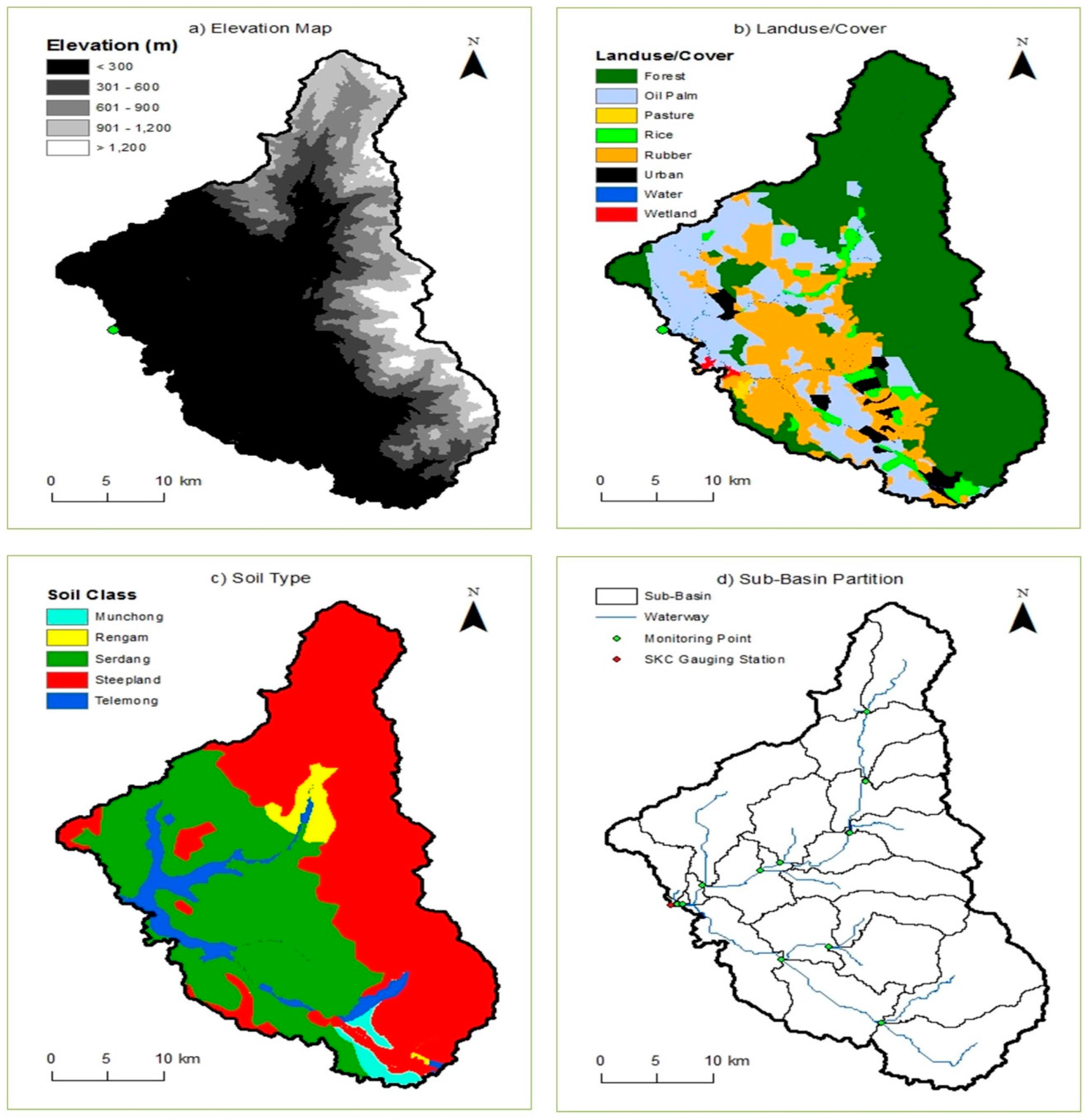
11] was performed using five scenarios to identify the effect of mixed land use change on the streamflow of the Bernam River basin. The results showed that land use changes are responsible for the increase in the annual flow depth between 8% and 39% during high flow months and decreases between 3% and 32% during low flow months, thus the need for best management practices as mitigative measures on future changes in land use on flow quantity. Table 1 and Figure 3 in [11] also show that the land use in this basin is changing based on data from 1984 to 2009. To-date, for instance, land use for oil palm has increase from 18.4% to 21.7% and rubber from 12.8% to 18.1%. Therefore, in our future studies, multiple GCMs and scenarios (including RCP2.6) and other downscaling methods would be employed to assess water shortage and allocation taking into account land use change scenarios within the basin. It is believed that the change of land use in the future will have a corresponding impact on streamflow.

5. Conclusions

The impact of climate change on the flows of the Upper Bernam River Basin in Malaysia was studied using the SWAT hydrological model. A graphical user interface was developed that integrates all of the common procedures of assessing climate change impacts, based on the delta method, to quickly simulate climate variables (e.g., rainfall, temperature, etc.) at the local scale from large-scale climate models. The interface is run with ten GCMs under three climate forcings. The tool was modified to generate future daily sequences by perturbing the baseline observed series using change factors derived from mean projected changes for that particular variable from climate models.
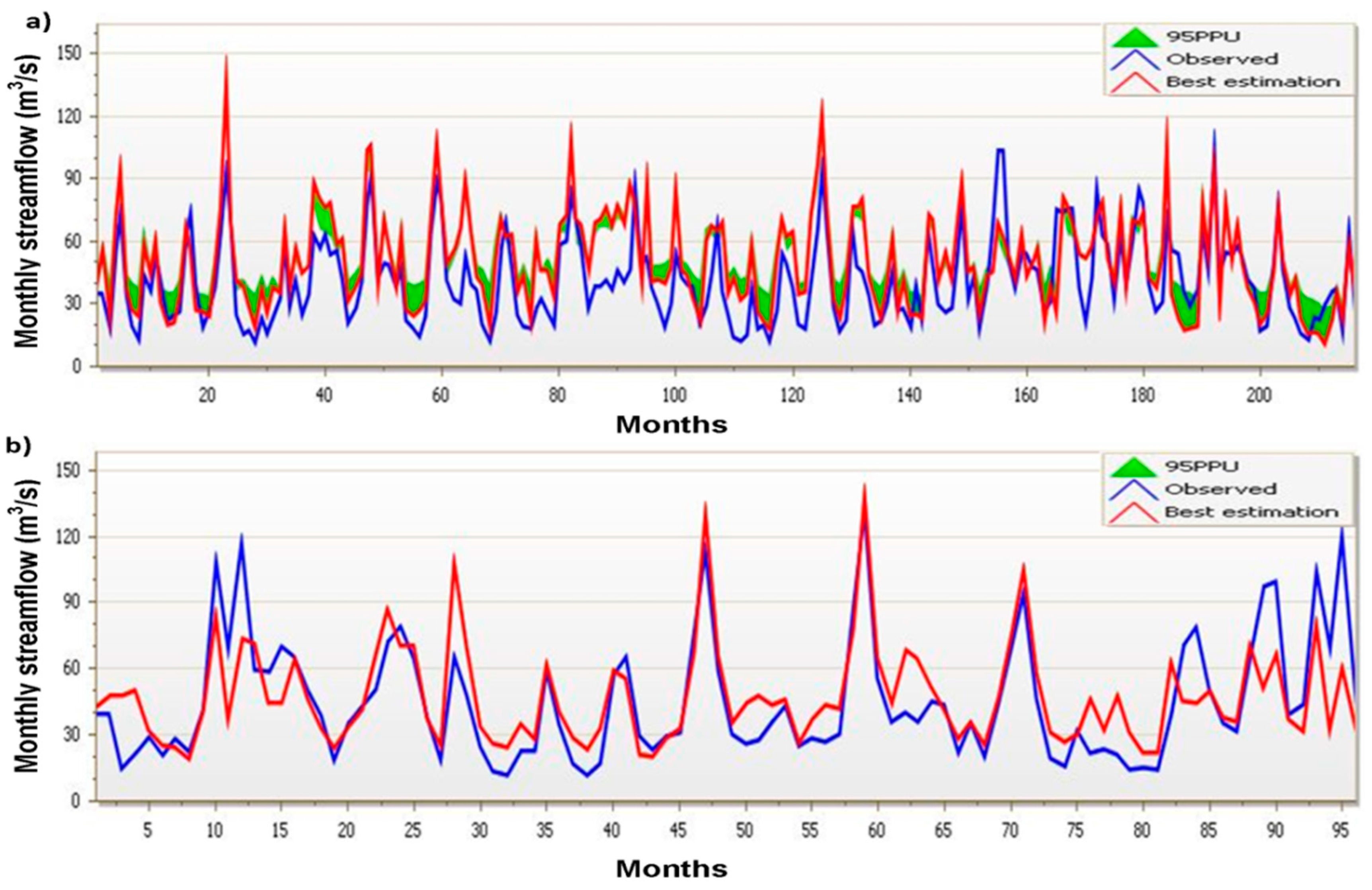
Climate variables influential for streamflow (mainly rainfall and temperature) were generated from the interface on the basis of the ten GCMs under RCP4.5, RCP6.0 and RCP8.5 and used as inputs to the SWAT hydrological model. This modeling study was carried out for the periods 2010–2039, 2050–2069 and 2070–2099 relative to the baseline period (1976–2005). The analysis was done on the basis of the rice farming seasons; dry (January–June) and wet (July–December). The evaluation results indicated that the hydrological model performed acceptably well in the study watershed with monthly R2, NSE and PBIAS values of 0.67, 0.62 and −9.4 and 0.62, 0.61 and −4.2 for the calibration and validation periods, respectively.
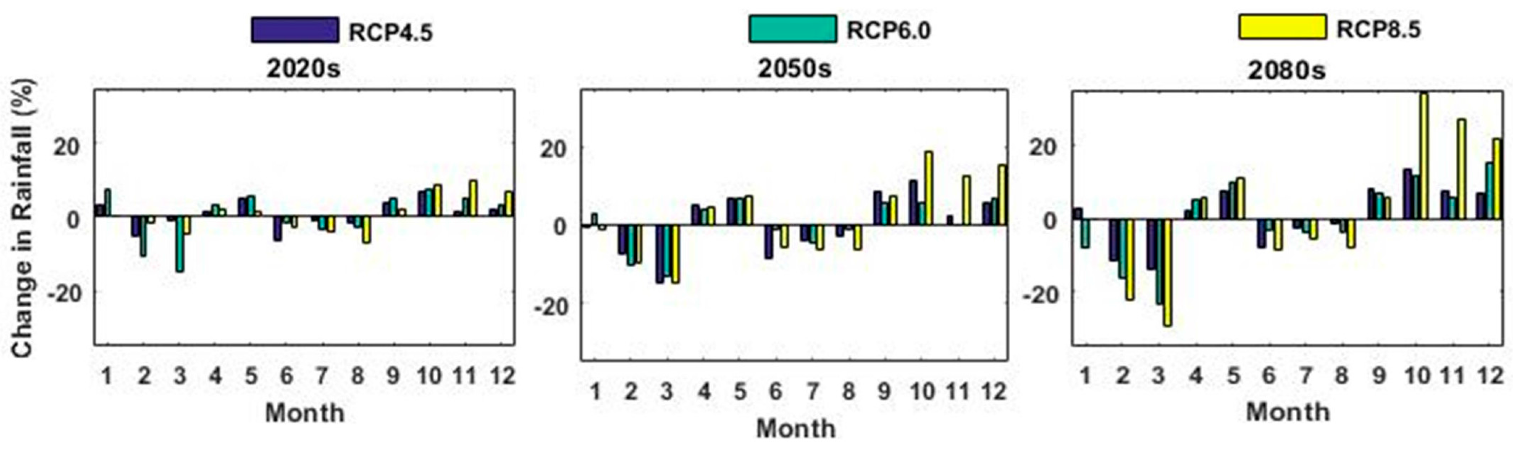
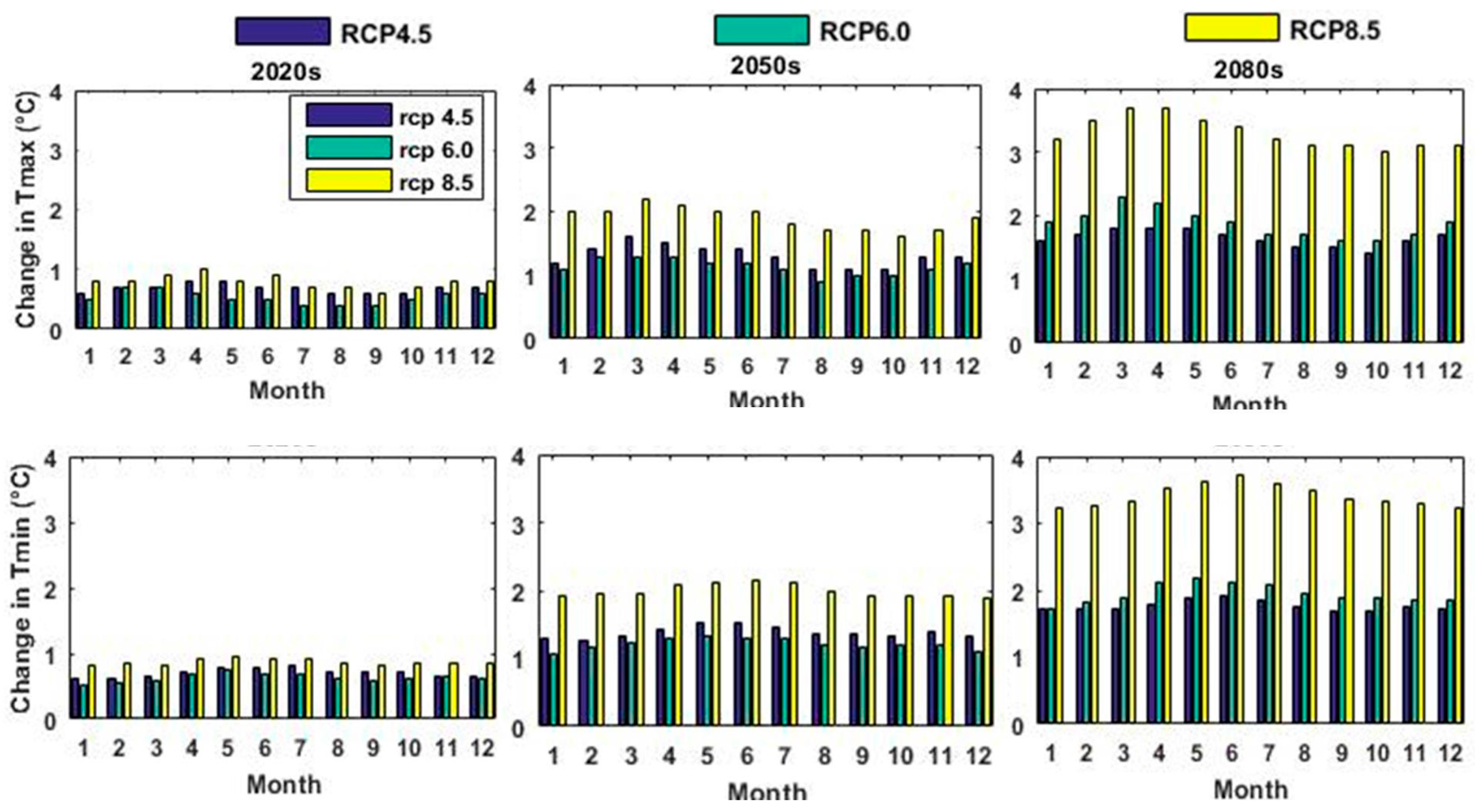
The multi-model projections indicated that the Upper Bernam River basin is likely to become warmer and wetter during some months in the future. Temperature is projected to increase in all respective scenarios. The largest monthly mean changes are observed during the dry season months (February–June) in all scenarios and are more significant under the most severe scenario, RCP8.5. Changes in rainfall showed variation between the two agricultural seasons (dry and wet) from the ensemble projections of the 10 GCMs. The dry season indicated a shortage in future rainfall with average changes of −2.4%, −3.2% and −3.7% under RCP4.5, 6.0 and 8.5, respectively. The wet season, on the other hand, is predicted to be wetter with average changes of about 1.0%, 0.8% and 2.4% for RCP4.5, 6.0 and 8.5, respectively. Overall annual future rainfall is likely to increase slightly with no significant changes from the baseline, although the monthly changes might affect rice water availability during the dry season and flooding in the wet season.
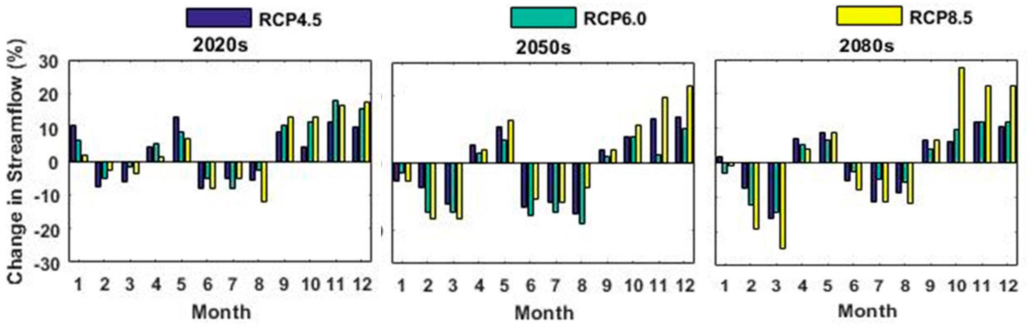
Streamflow projections followed that of rainfall to a great extent with a distinct change between the dry and wet season. Generally, all future periods show a decreasing trend in streamflow during this season and an increasing pattern in the wet season. The significant decrease (−6.6%) occurs under the RCP8.5 scenario in the late century (2080s), while a significant increase of 11.4% occurs in the same future period under the same scenario. On the basis of these results, it can be inferred that the water resource of the Bernam River Basin may be sufficient up to the end of the century, since the projected decreases are counteracted by the increases. However, the basin may experience tremendous pressure due to low flows during the dry season and flooding during the wet season. Thus, it necessitates integrated water resources solutions to ensure water availability for rice production at all times and mitigative measures against flooding risk. It can be concluded that the interface is user friendly and can, in principle, be customized for application to other geographical areas or catchments by incorporating baseline data for those particular stations of the new catchment area and their corresponding GCMs’ outputs, for the quick generation of climate variables for hydrological assessment and/or as inputs to crop models.

Acknowledgments

The authors wish to acknowledge the Ministry of Higher Education in Malaysia (MOHE) and Universiti Putra Malaysia (UPM) for providing funding for this research. This research is funded by the Universiti Putra Malaysia under Putra Grant 9406300 and the Ministry of Higher Education (MOHE) under Fundamental Research Grant Scheme (FRGS): 5524362. We are grateful to the staff of the Department of Irrigation and Drainage (DID) and the National Hydraulic Research Institute of Malaysia (NAHRIM) for providing hydro-meteorological data. Sincere appreciation is also extended to the reviewers for their valuable critiques and recommendations in improving this manuscript.

Author Contributions

Nkululeko Simeon Dlamini is a postgraduate student, who worked on downloading the GCM data from the website, downscaling using MATLAB programming and running future simulations on the SWAT model. Rowshon Kamal is the corresponding author, who has given scholastic and valuable comments, reviewed the manuscript and designed the user-interface development. He is also the supervisor and the leader of the sponsored projects for this study. Mohd Amin Bin Mohd Soom edited the final manuscript. Mohd Syazwan Faisal bin Mohd provided data and the technical support for the calibration and validation of the SWAT model. The remaining co-authors were involved in the project. They gave valuable comments and reviewed the analysis of the future streamflow outputs to ensemble projections. All of them are members of the supervisory committee, except Mohd Syazwan Faisal bin Mohd.

Conflicts of Interest

The authors declare no conflict of interest.

References

  1. Solomon, S. Climate Change 2007—The Physical Science Basis: Working Group I Contribution to the Fourth Assessment Report of the IPCC (Vol. 4); Cambridge University Press: Cambridge, UK, 2007. [Google Scholar]
  2. Wilby, R.; Charles, S.; Zorita, E.; Timbal, B.; Whetton, P.; Mearns, L. Guidelines for Use of Climate Scenarios Developed from Statistical Downscaling Methods, IPCC Task Group on Scenarios for Climate Impact Assessment (TGCIA). Availiable online: www.ipcc-data.org/guidelines/dgm_no2_v1_09_2004.pdf (accessed on 4 August 2014).
  3. Xu, C.Y. Climate change and hydrologic models: A review of existing gaps and recent research developments. Water Resour Manag. 1999, 13, 369–382. [Google Scholar] [CrossRef]
  4. Stocker, T. Climate Change 2013: The Physical Science Basis: Working Group I Contribution to the Fifth Assessment Report of the Intergovernmental Panel on Climate Change; Cambridge University Press: Cambridge, UK, 2014. [Google Scholar]
  5. Alam, M.M.; Siwar, C.; Molla, R.I.; Talib, B.; Bin Toriman, M.E. Paddy farmers’ adaptation practices to climatic vulnerabilities in Malaysia. Mitig. Adapt. Strateg. Glob. Chang. 2012, 17, 415–423. [Google Scholar] [CrossRef]
  6. Tan, M.L.; Ficklin, D.L.; Yusop, Z. Impacts and uncertainties of climate change on streamflow of the Johor River Basin, Malaysia using a CMIP5 General Circulation Model ensemble. J. Water Clim. Chang. 2014, 5, 676–695. [Google Scholar] [CrossRef]
  7. Fowler, H.; Blenkinsop, S.; Tebaldi, C. Linking climate change modelling to impacts studies: Recent advances in downscaling techniques for hydrological modelling. Int. J. Climatol. 2007, 27, 1547–1578. [Google Scholar] [CrossRef]
  8. Prudhomme, C.; Reynard, N.; Crooks, S. Downscaling of global climate models for flood frequency analysis: Where are we now? Hydrol. Process. 2002, 16, 1137–1150. [Google Scholar] [CrossRef]
  9. Ghazalli, M. Modernisation of Irrigation and Drainage Management for Agricultural Production; Department of Irrigation and Drainage Malaysia: Kuala Lumpur, Malaysia, 1998. [Google Scholar]
  10. Lee, T.S.; Haque, M.A.; Najim, M. Scheduling the cropping calendar in wet-seeded rice schemes in Malaysia. Agric. Water Manag. 2005, 71, 71–84. [Google Scholar] [CrossRef]
  11. Alansi, A.; Amin, M.; Abdul Halim, G.; Shafri, H.; Aimrun, W. Validation of SWAT model for stream flow simulation and forecasting in Upper Bernam humid tropical river basin, Malaysia. Hydrol. Earth Syst. Sci. Discuss. 2009, 6, 7581–7609. [Google Scholar] [CrossRef]
  12. Prudhomme, C.; Jakob, D.; Svensson, C. Uncertainty and climate change impact on the flood regime of small UK catchments. J. Hydrol. 2003, 277, 1–23. [Google Scholar] [CrossRef]
  13. Dibike, Y.B.; Coulibaly, P. Hydrologic impact of climate change in the Saguenay watershed: Comparison of downscaling methods and hydrologic models. J. Hydrol. 2005, 307, 145–163. [Google Scholar] [CrossRef]
  14. Jones, R.; Murphy, J.; Noguer, M.; Keen, A. Simulation of climate change over Europe using a nested regional-climate model. II: Comparison of driving and regional model responses to a doubling of carbon dioxide. Q. J. R. Meteorol. Soc. 1997, 123, 265–292. [Google Scholar] [CrossRef]
  15. Mearns, L.; Giorgi, F.; Whetton, P.; Pabon, D.; Hulme, M.; Lal, M. Guidelines for Use of Climate Scenarios Developed from Regional Climate Model Experiments. Data Distribution Centre of the Intergovernmental Panel on Climate Change, IPCC Task Group on Scenarios for Climate Impact Assessment (TGCIA). Available online: www.ipcc-data.org/guidelines/dgm_no1_v1_10-2003.pdf (accessed on 4 August 2014).
  16. Wilby, R.L.; Hassan, H.; Hanaki, K. Statistical downscaling of hydrometeorological variables using general circulation model output. J. Hydrol. 1998, 205, 1–19. [Google Scholar] [CrossRef]
  17. Chung, S.O.; Rodríguez-Díaz, J.; Weatherhead, E.; Knox, J. Climate change impacts on water for irrigating paddy rice in South Korea. Irrig. Drain. 2011, 60, 263–273. [Google Scholar] [CrossRef]
  18. Dessu, S.B.; Melesse, A.M. Impact and uncertainties of climate change on the hydrology of the Mara River basin, Kenya/Tanzania. Hydrol. Process. 2013, 27, 2973–2986. [Google Scholar] [CrossRef]
  19. Diaz-Nieto, J.; Wilby, R.L. A comparison of statistical downscaling and climate change factor methods: Impacts on low flows in the River Thames, United Kingdom. Clim. Chang. 2005, 69, 245–268. [Google Scholar] [CrossRef]
  20. Nakicenovic, N.; Swart, R. Special Report on Emissions Scenarios Edited by Nebojsa Nakicenovic and Robert Swart; Cambridge University Press: Cambridge, UK, 2000; p. 612. ISBN 0521804930. [Google Scholar]
  21. Meinshausen, M.; Smith, S.J.; Calvin, K.; Daniel, J.S.; Kainuma, M.; Lamarque, J.; Riahi, K. The RCP greenhouse gas concentrations and their extensions from 1765 to 2300. Clim Chang. 2011, 109, 213. [Google Scholar] [CrossRef]
  22. Wayne, G. The Beginner’s Guide to Representative Concentration Pathways. 2013. Available online: https://skepticalscience.com/docs/RCP_Guide.pdf (accessed on 7 January 2015).
  23. Gassman, P.; Reyes, M.; Green, C.; Arnold, J. The soil and water assessment tool: Historical development, applications, and future research directions Invited Review Series. Trans. Am. Soc. Agric. Eng. 2007, 50, 1211–1250. [Google Scholar]
  24. Deni, S.M.; Jemain, A.A. Fitting the distribution of dry and wet spells with alternative probability models. Meteorol. Atmos. Phys. 2009, 104, 13–27. [Google Scholar] [CrossRef]
  25. The study on Modernization of Irrigation Water Management System in the Granary Areas of Peninsular Malaysia. In Nippon Koei, Kuala Lumpur, Malaysia; JICA, DID: Kuala Lumpur, Malaysia, 1998.
  26. Wong, C.; Venneker, R.; Jamil, A.; Uhlenbrook, S. Development of a gridded daily hydrometeorological data set for Peninsular Malaysia. Hydrol. Process. 2011, 25, 1009–1020. [Google Scholar] [CrossRef]
  27. Wong, C.; Venneker, R.; Uhlenbrook, S.; Jamil, A.; Zhou, Y. Variability of rainfall in Peninsular Malaysia. Hydrol. Earth Syst. Sci. Discuss. 2009, 6, 5471–5503. [Google Scholar] [CrossRef]
  28. Lai, S.H. Application of Swat Hydrological Model with GIS Interface to Upper Bernam River Basin. Unpublished Thesis, Universiti Putra Malaysia, Serdang, Selangor, 2001. [Google Scholar]
  29. Wong, I.F. Reconnaissance Soil Survey of Selangor; Ministry of Agriculture and Lands, Division of Agriculture: Putrajaya, Malaysia, 1970. [Google Scholar]
  30. Babel, M.S.; Wahid, S.M. Freshwater Under Threat South East Asia: Vulnerability Assessment of Freshwater Resources to Environmental Change: Mekong River Basin. United Nations Environment Programme (UNEP): Nairobi, Kenya, 2009. Available online: http://www.unep.org/pdf/southasia_report.pdf (accessed on 7 January 2015).
  31. Raneesh, K.; Thampi Santosh, G. A study on the impact of climate change on streamflow at the watershed scale in the humid tropics. Hydrol. Sci. J. 2011, 56, 946–965. [Google Scholar] [CrossRef]
  32. Neitsch, S.L.; Arnold, J.G.; Kiniry, J.R.; Williams, J.R. Soil and Water Assessment Tool Theoretical Documentation Version 2009; Texas Water Resources Institute: College Station, TX, USA, 2011. [Google Scholar]
  33. Arnold, J.G.; Srinivasan, R.; Muttiah, R.S.; Williams, J.R. Large Area Hydrologic Modeling and Assessment Part I: Model Development 1; Wiley Online Library: Hoboken, NJ, USA, 1998. [Google Scholar]
  34. Eckhardt, K.; Arnold, J. Automatic calibration of a distributed catchment model. J. Hydrol. 2001, 251, 103–109. [Google Scholar] [CrossRef]
  35. Williams, J.R. Flood routing with variable travel time or variable storage coefficients. Trans. Am. Soc. Civ. Eng. 1969, 12, 100–103. [Google Scholar] [CrossRef]
  36. Arnold, J.G.; Moriasi, D.N.; Gassman, P.W.; Abbaspour, K.C.; White, M.J.; Srinivasan, R.; van Liew, M.W. SWAT: Model use, calibration, and validation. Trans. Am. Soc. Agric. Eng. 2012, 55, 1491–1508. [Google Scholar]
  37. Abbaspour, K.C.; Yang, J.; Maximov, I.; Siber, R.; Bogner, K.; Mieleitner, J.; Srinivasan, R. Modelling hydrology and water quality in the pre-alpine/alpine Thur watershed using SWAT. J. Hydrol. 2007, 333, 413–430. [Google Scholar] [CrossRef]
  38. Abbaspour, K.; Johnson, C.; van Genuchten, M.T. Estimating uncertain flow and transport parameters using a sequential uncertainty fitting procedure. Vadose Zone J. 2004, 3, 1340–1352. [Google Scholar] [CrossRef]
  39. Yang, J.; Reichert, P.; Abbaspour, K.; Xia, J.; Yang, H. Comparing uncertainty analysis techniques for a SWAT application to the Chaohe Basin in China. J. Hydrol. 2008, 358, 1–23. [Google Scholar] [CrossRef]
  40. Ashraf Vaghefi, S.; Mousavi, S.; Abbaspour, K.; Srinivasan, R.; Yang, H. Analyses of the impact of climate change on water resources components, drought and wheat yield in semiarid regions: Karkheh River Basin in Iran. Hydrol. Process. 2014, 28, 2018–2032. [Google Scholar] [CrossRef]
  41. Santhi, C.; Arnold, J.G.; Williams, J.R.; Dugas, W.A.; Srinivasan, R.; Hauck, L.M. Validation of the SWAT model on a large river basin with point and nonpoint sources. J. Am. Water Resour. Assoc. 2001, 37, 1169–1188. [Google Scholar] [CrossRef]
  42. Van Liew, M.; Arnold, J.; Garbrecht, J. Hydrologic simulation on agricultural watersheds: Choosing between two models. Trans. Am. Soc. Civ. Eng. 2003, 46, 1539–1551. [Google Scholar] [CrossRef]
  43. Gupta, H.V.; Sorooshian, S.; Yapo, P.O. Status of automatic calibration for hydrologic models: Comparison with multilevel expert calibration. J. Hydrol. Eng. 1999, 4, 135–143. [Google Scholar] [CrossRef]
  44. Moriasi, D.N.; Arnold, J.G.; van Liew, M.W.; Bingner, R.L.; Harmel, R.D.; Veith, T.L. Model evaluation guidelines for systematic quantification of accuracy in watershed simulations. Trans. Am. Soc. Agric. Eng. 2007, 50, 885–900. [Google Scholar]
  45. Ghosh, S.; Mujumdar, P. Nonparametric methods for modeling GCM and scenario uncertainty in drought assessment. Water Resour. Res. 2007, 43. [Google Scholar] [CrossRef]
  46. New, M.; Hulme, M. Representing uncertainty in climate change scenarios: A Monte-Carlo approach. Integr. Assess. 2000, 1, 203–213. [Google Scholar] [CrossRef]
  47. Chen, J.; Brissette, F.P.; Leconte, R. Uncertainty of downscaling method in quantifying the impact of climate change on hydrology. J. Hydrol. 2011, 401, 190–202. [Google Scholar] [CrossRef]
  48. Ouyang, F.; Zhu, Y.; Fu, G.; Lü, H.; Zhang, A.; Yu, Z.; Chen, X. Impacts of climate change under CMIP5 RCP scenarios on streamflow in the Huangnizhuang catchment. Stoch. Environ. Res. Risk Assess. 2015, 29, 1781–1795. [Google Scholar] [CrossRef]
  49. Knox, J.W.; Díaz, J.R.; Nixon, D.; Mkhwanazi, M. A preliminary assessment of climate change impacts on sugarcane in Swaziland. Agric. Syst. 2010, 103, 63–72. [Google Scholar] [CrossRef] [Green Version]
  50. Lelis, T.A.; Calijuri, M.L.; Santiago, A.D.F.; Lima, D.C.D.; Rocha, E.D.O. Sensitivity analysis and calibration of SWAT model applied to a watershed in southeastern Brazil. Rev. Bras. Ciênc. Solo 2012, 36, 623–634. [Google Scholar] [CrossRef]
  51. Pinto, D.B.F.; da Silva, A.M.; Beskow, S.; de Mello, C.R.; Coelho, G. Application of the soil and water assessment tool(swat) for sediment transport simulation at a headwater watershed in Minas Gerais State, Brazil. Trans. Am. Soc. Agric. Eng. 2013, 56, 697–709. [Google Scholar]
  52. Kilsby, C.; Jones, P.; Burton, A.; Ford, A.; Fowler, H.; Harpham, C.; Wilby, R. A daily weather generator for use in climate change studies. Environ. Model. Softw. 2007, 22, 1705–1719. [Google Scholar] [CrossRef]
Figure 1. Map of study area: Upper Bernam watershed, Malaysia.
Water 09 00226 g001
Figure 2. Framework of the study for the assessment of climate change impacts on future flows of the Bernam River Basin. NS, Nash–Sutcliffe; PBIAS, Percent Bias.
Water 09 00226 g002
Figure 3. Bernam watershed delineation process in the SWAT model.
Water 09 00226 g003
Figure 4. Spatial input data in the SWAT model for Bernam River Basin, including: (a) Digital Elevation Model (DEM) at 30-m resolution; (b) reclassified land use dataset; (c) soils dataset from DOA; (d) sub-basins’ partition.
Water 09 00226 g004
Figure 5. Dialog main window of the hydro-meteorological interface for the simulation of climate data in the Bernam River catchment area.
Water 09 00226 g005
Figure 6. Schematic flowchart for the simulation of climate sequences in the hydro-meteorological interface under climate forcing.
Water 09 00226 g006
Figure 7. Example of a one-year simulation of daily sequences of climate variables using the CCSM4 model under the RCP4.5 scenario (1 January–31 December 2017).
Water 09 00226 g007
Figure 8. Example of a one-year simulation of daily rainfall sequences using the CCSM4 model under the RCP4.5 scenario (1 January–31 December 2017).
Water 09 00226 g008
Figure 9. Mean monthly changes in temperatures (tmax and tmin (°C) for the future years (2020s, 2050s and 2080s)) under the RCP4.5, 6.0 and 8.5 scenarios.
Water 09 00226 g009
Figure 10. Example of the mean monthly changes in future temperature maximum (tmax) under the RCP45 scenario generated from the interface.
Water 09 00226 g010
Figure 11. Mean monthly changes in rainfall (°C) for the future years (2020s, 2050s and 2080s) under the RCP4.5, 6.0 and 8.5 scenarios compared with the baseline period (1976–2005).
Water 09 00226 g011
Figure 12. Plot of the observed and simulated streamflow for the calibration (1981–1998) and validation (1999–2006) periods at SKC station.
Water 09 00226 g012
Figure 13. Average projected changes of monthly streamflow for the 2020s, 2050s and 2080s under RCP4.5, RCP6.0 and RCP8.5, with respect to the baseline simulation (1976–2005).
Water 09 00226 g013
Table 1. Summary of the input dataset for flow modeling of Bernam River Basin.
DataData SourceData Description
Digital Elevation Model (DEM)DIVA-GIS (GIS Data Depository Organization)Elevation, overland, channel slopes, boundary
Soils MapDepartment of Agriculture (DOA)Soil classification and properties
Land Use MapDepartment of Agriculture (DOA)Land use classification: cropland, forest, pastures, etc.
Climate DataDepartment of Irrigation and Drainage (DID)Daily rainfall, maximum and minimum temperature (1976–2005)
StreamflowDepartment of Irrigation and Drainage (DID)Daily stream outflow (1975–2006)
Table 2. List of Global Climate Models used in this study.
OrganizationGCMResolution
LatitudeLongitude
Canadian Centre for Climate Modelling and AnalysisCanESM22.82.8
National Center for Atmospheric ResearchCCSM41.250.94
Centre National de Recherches Météorologiques/Centre Européen de Recherche et Formation Avancée en CalculScientifiqueCNRM-CM51.41.4
Commonwealth Scientific and Industrial Research Organization in collaboration with Queensland Climate Change Centre of ExcellenceCSIRO1.81.8
NOAA Geophysical Fluid Dynamics LaboratoryGFDL-ESM2G2.52.0
NOAA Geophysical Fluid Dynamics LaboratoryGFDL-ESM2M2.52.0
Met Office Hadley CentreHadGEM2-CC1.881.25
Met Office Hadley Centre HadGEM2-ES1.881.25
Max-Planck-Institutfür Meteorologie (Max Planck Institute for Meteorology)MPI-ESM-LR1.881.87
Meteorological Research InstituteMRI-CGCM31.11.1
Notes: Canadian Earth System Model (CanESM2); Community Climate System Model (CCSM4); Centre National de RecherchesMétéorologiques/Centre Européen de Recherche et Formation Avancée en CalculScientifique (CNRM-CM5); Commonwealth Scientific and Industrial Research Organization (CSIRO); Coupled Global Climate Model (CGCM3); Max Planck Institute for Meteorology (MPI-M), the new Earth system model (MPI-ESM-LR); Hadley Global Environment Model 2—Earth System (HadGEM2-ES); Hadley Global Environment Model 2—Carbon Cycle (HadGEM2-CC); Earth System Models using Generalized Ocean Layer Dynamics (ESM2G); Earth System Models using the Modular Ocean Model (GFDL-ESM2M).
Table 3. Annual changes in future tmax, tmin and rainfall under the RCP45, 60 and 85 scenarios.
PeriodsAnnual Changes Corresponding to Scenarios
RCP4.5RCP6.0RCP8.5
Maximum temperature (°C)
2020s0.70.50.8
2050s1.31.11.9
2080s1.61.93.3
Minimum temperature (°C)
2020s0.70.60.9
2050s1.41.22.0
2080s1.81.93.4
Table 4. Annual changes in future rainfall under the RCP45, 60 and 85 scenarios.
PeriodsAnnual Changes Corresponding to Scenarios
RCP4.5RCP6.0RCP8.5
Average change (Dry season)−2.4−3.2−3.7
2020s−0.4−1.8−0.7
2050s−3.2−1.8−3.3
2080s−3.6−6.1−7.1
Average change (Wet season)1.00.82.4
2020s2.02.52.7
2050s0.20.21.8
2080s0.9−0.42.7
Average change (Annual)
2020s0.80.41.0
2050s0.20.21.8
2080s0.9−0.42.7
Note: Rice farming seasons: (1) dry season: (January–June); (2) wet season: (July–December).
Table 5. SWAT parameter changes during calibration stage.
RankParameters DescriptionFileFinal Parameter Range
Min Max
1CN2 (SCS curve number).mgt−0.30000.3000
2ALPHA_BF (Baseflow alpha factor).gw0.00001.0000
3ESCO (Soil evaporation compensation factor).hru0.00001.0000
4GW_REVAP (Groundwater revap coefficient).gw0.00000.4000
5CH_N2 (Manning’s value for main channel).rte0.00000.3000
6SOL_BD (Soil bulk density).sol−0.02700.3000
7GW_DELAY (Groundwater delay).gw30.000450.00
8GWQMN (Threshold water depth in the shallow aquifer for flow).gw0.00001.8800
9CH_K2 (Channel effective hydraulic conductivity).rte4.0000130.00
Table 6. Annual changes in future streamflow under the RCP45, 60 and 85 scenarios.
PeriodsSeasonal Changes Corresponding to Scenarios
RCP4.5RCP6.0RCP8.5
Dry season−1.5−2.8−4.3
2020s1.11.3−0.9
2050s−3.6−6.4−5.3
2080s−2.0−3.4−6.6
Wet season4.45.09.4
2020s5.29.58.5
2050s3.90.08.4
2080s4.35.311.4
Annual
2020s2.54.43.1
2050s−0.8−4.00.5
2080s0.10.51.3
Note: Rice farming seasons: (1) dry season: (January–June); (2) wet season: (July–December).

