Article

Quantitative Spatio-Temporal Characterization of Scour at the Base of a Cylinder

1
Water Unit, AECOM, Houston, TX 77094, USA
2
Department of Civil and Environmental Engineering, Lehigh University, Bethlehem, PA 18015, USA
3
Department of Mechanical Engineering, Virginia Tech, Blacksburg, VA 24061, USA
4
Department of Civil and Environmental Engineering, Virginia Tech, Blacksburg, VA 24061, USA
*
Author to whom correspondence should be addressed.
Water 2017, 9(3), 227; https://doi.org/10.3390/w9030227
Submission received: 10 January 2017 / Revised: 8 March 2017 / Accepted: 16 March 2017 / Published: 20 March 2017
(This article belongs to the Special Issue Stream Channel Stability, Assessment, Modeling, and Mitigation)

Abstract

:
The measurement of the morphologic characteristics of evolving sediment beds around hydraulic structures is crucial for the understanding of the physical processes that drive scour. Although there has been significant progress towards the experimental characterization of the flow field in setups with complex geometries, little has been done with respect to the quantitative investigation of dynamic sediment bed geometry, mainly due to the limited capabilities of conventional instrumentation. Here, a recently developed computer vision technique is applied to obtain high-resolution topographic measurements of the evolving bed at the base of a cylinder during clear water scour, without interrupting the experiment. The topographic data is processed to derive the morphologic characteristics of the bed such as the excavated volume and the slopes of the bed. Subsequently, the rates of scour and the bathymetry at multiple locations are statistically investigated. The results of this investigation are compared with existing flow measurements from previous studies to describe the physical processes that take place inside a developing scour hole. Two distinct temporal phases (initial and development) as well as three spatial regions (front, side and wake) are defined and expressions for the statistical modelling of the bed features are derived.

1. Introduction

The interaction among hydraulic structures, water flows and sediment beds is one of the most complicated phenomena in hydraulic engineering. The prediction of changes in the bed topography due to scour is fundamental for the safe and cost-effective design of hydraulic structures [1]. This problem has been extensively investigated over the last decades through numerous laboratory tests, field observations, numerical simulations, and derivation of empirical relationships. The main focus of the majority of these studies has been the prediction of the maximum scour depth after several hours or even days of testing, when equilibrium conditions have been reached. Fewer studies have focused on the temporal evolution of the instantaneous maximum scour depth. Many of the derived empirical or semi-empirical relationships were recently summarized and evaluated in [2]. Although these efforts have provided us with important insights on the effects of various parameters on the scour depth in laboratory simulations, physical understanding of the phenomenon is incomplete. Consequently, improved engineering tools are needed to advance the design and protection of hydraulic structures.
In an effort to better understand the physics behind scour, fluid flows around wall-mounted obstacles, such as cylinders or wings, have been described from experimental observations [3,4,5,6] or numerical simulations [7,8,9]. These studies examined the time-averaged and time-resolved characteristics of flows around the obstacles. Coherent vortices forming at the face of the obstacles and periodically shedding vortices at the wake of these obstacles were identified as the main agents that drive scour.
In order to examine directly the interaction between the flow, the structure and the channel bed, experiments of flows over erodible boundaries have been carried out by several researchers. However, the laboratory investigation of these cases presents important challenges that usually compromise the resolution and reliability of the measurements. Consequently, many of these studies focus on the description of the flow over static beds that have either been artificially stabilized, or have reached equilibrium conditions [10,11,12,13,14]. However, artificially stabilized beds provide a nearly static representation of the actual dynamic phenomenon and therefore do not allow for the study of the evolving scour hole due to the complex interaction between the flow, the structure and the channel bed. Also, many researchers agree that equilibrium is not representative of the conditions in the field, due to the very long duration of floods that are required to approach it [15,16,17]. Furthermore, recent studies have shown that the morphodynamics of the scour hole depend greatly on the shape of the hydrograph [18]; thus the examination of scour under steady-discharge flows of very long durations do not describe accurately the effects of real-life floods.
In some other cases, time-resolved measurements of the bed have been carried out by measuring the bathymetry of the bed at one or a few locations within the scour hole [15,19,20]. This is usually accomplished with acoustic or laser range finders, or simpler methods such as the recording of measuring scales attached to the model structure. These measurements can be useful for the derivation of relationships between time and scour depth; yet, more detailed measurements that capture the morphological characteristics of the entire scour hole evolution in time are necessary for obtaining further insight on the physics of the phenomenon. Additionally, detailed representations of the scour hole have been obtained with photogrammetric [21] or laser-based techniques [22] that are capable of high-spatial resolution measurements. However, to use these techniques it was necessary to stop the experiment and drain the flume.
In a few cases the evolving topography of the scour hole has been investigated without interrupting the experiment. For example, in [23,24] an image-processing technique was employed to study the kinematics of the mobile sediment within a scour hole around an abutment. They recorded the sediment bed through a transparent window that was covering the surface of the flow to observe how the patterns of sediment transport vary as scour grows. Also, in [25] a laser range finder was mounted on a motorized carriage inside a transparent cylinder and obtained multiple bathymetric measurements within an evolving scour hole. In their study, complete topographies were measured in an asynchronous manner using 30–180 s per topography scan and a few of them were presented to discuss some morphological characteristics of the bed, such as volumes and slopes around the scour hole. Additionally, [26] presented the evolving centerline profile upstream and downstream of a cylinder, at the initial instants of scour and included an extensive discussion about the characteristics of the flow and corresponding bathymetric profiles. In this important contribution, however, the discussion about various bed features was mainly qualitative in nature.
Thorough descriptions of the evolving morphological characteristics of the bed and correlations with the flow are provided in recent numerical simulations in [27,28,29]. These groups carried out coupled modelling of the flow characteristics and the bed evolution in an effort to identify the cause and effect relationships that drive scour. Their models were validated with the findings of [26] or with basic laboratory measurements that they carried out themselves.
Based on the measurements, simulations, and visual observations available in existing studies, several descriptions have been provided about the phenomena that take place inside developing scour holes and empirical descriptions of this complicated phenomenon have been proposed. Although reasonable, some of these empirical descriptions are not fully supported by detailed experimental measurements.
Here we describe the morphological characteristics of an evolving gravel bed around a circular cylinder, under clear-water scour conditions at a laboratory scale. We have employed a recently developed computer vision technique [30] to overcome the limitations of existing instrumentation and measure accurately, continuously and non-intrusively the development of the scour hole topography at very high spatial and temporal resolution. Such measurements avoid the disturbances introduced by stopping and restarting the experiment and the impact of intrusive measuring technologies, both of which can alter the outcome of the experiment. Contrary to the vast majority of existing bridge scour studies that presented limited morphological features obtained from several experiments, here the dynamic scour hole morphology is examined thoroughly for a simple, yet broadly representative experimental case. The results are physically interpreted and compared with descriptions of the flow and bed characteristics that have been presented in previous studies, to investigate the main mechanisms of scour.
The experimental parameters and the measuring technique are described in the next section. The evolving topographic features, scour rates, slopes and volume of the scour hole are presented and discussed in Section 3. In Section 4, the overall results are considered in an effort to associate the findings with expected flow characteristics and describe physically the phenomenon. Finally, the main conclusions are summarized in Section 5.

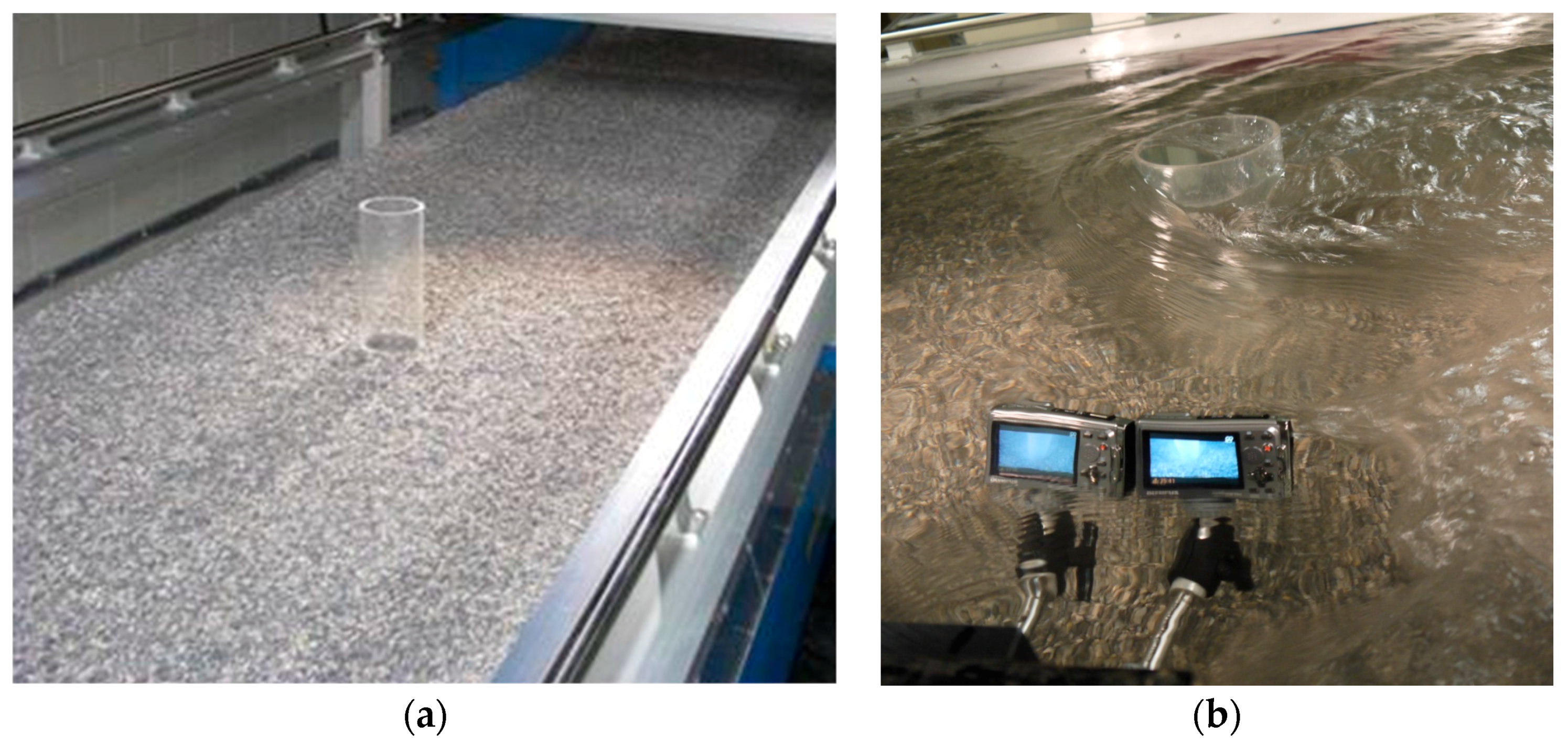
2. Experimental Set Up and Data Collection

The main objective of this work was to study the scour development process around a circular pier with an unprecedented degree of detail. To meet this objective and allow for the comparison of the current work with results obtained from previous studies, a simple, yet broadly representative experimental case was considered here. The experiment was carried out in a flume 16.2-m long and 1.2-m wide, with slope (S) equal to 0.0005 (Figure 1a). The bed material was uniform crushed gravel with median diameter, d50 = 3.55 mm, geometric standard deviation, σ = 1.35, and angle of repose, φ = 35°. The approach flow depth, H, was 0.205 m, the approach depth-averaged flow velocity (V) was 0.620 m/s, and the water temperature (T) was 25 °C. The model pier was a circular cylinder with diameter, D, equal to 0.152 m. The cylinder was mounted on the center of the flume approximately 50 flow depths downstream of its entrance to ensure that the flow was fully developed [31]. The experiment lasted for 250 min. The most relevant dimensionless parameters of the experiment are: τ/τc = 0.95, H/D = 1.35, D/d50 = 43, ReD = 81,000, ReH = 109,000, Fr = 0.44; where τ: bed shear stress; τc: critical bed shear stress for sediment entrainment, ReD: pier diameter-based Reynolds number (ReD = VD/ν, ν: kinematic viscosity), ReH: approach flow depth-based Reynolds number (ReH = VH/ν), and Fr: Froude number (Fr = V/(gH)0.5, g: gravitational acceleration). The critical shear stress (τc) was found experimentally by the gradual increase of the flow velocity and the observation of the flume for sporadic sediment entrainment.
For the monitoring of the channel bed evolution in the vicinity of the pier, two waterproof cameras (Olympus Stylus Tough—6020, Olympus Corporation, Tokyo, Japan) were used. The cameras were mounted firmly on the sidewalls of the flume close to the test section, as shown in Figure 1b, and were recording videos at 30 frames per second, with resolution equal to 720 × 1280 pixels, while being partially submerged. The dimensions of the cameras were 100 × 65 × 26 mm. The purpose was to record the lateral half of the scour hole and assume symmetry about the centerline of the flume. In that area every 1 cm2 was represented by more than 6500 pixels. The distance of the cameras from the bed and the cylinder were approximately 180 mm and 400 mm, respectively. Before the beginning of the experiment, water was introduced gradually, while an adjustable tailgate at the downstream end of the flume was raised. As soon as the flow reached the desired depth, the cameras were synchronized using a stroboscopic light, and started recording videos. The target velocity was reached by adjusting the flow discharge and the tailgate. At the completion of the experiment, the flow discharge was reduced and the tailgate was raised. Before draining the flume, the velocity of the flow was greatly decreased and the bed bathymetry was measured with a point gauge to validate the accuracy of the primary measurements.
The recorded videos were processed in Matlab by applying a computer-vision based technique that was recently developed in [30]. The inputs for this technique are the two synchronized videos of the evolving bed and the final outputs are the 3D representations of the bed topography at multiple instants. This is achieved by the implementation of a series of algorithms that perform calibration of the cameras and stereo-triangulation to derive 3D surfaces. The maximum temporal resolution of the measurements was 30 reconstructed surfaces per second. An area of approximately 140 cm2 of the bed was represented by more than 6000 points at every instant. The accuracy of the measurements was 0.86 mm and the precision was 2.31 mm. The detailed description of the technique along with investigations of its accuracy and reliability are presented in [30]. Overall, this methodology allows for the continuous collection of very high temporal and spatial resolution measurements of the bed topography, while being minimally intrusive. Though numerous experiments using similar configurations have been carried out in the past, this is the first time, to the authors’ knowledge, that such high quality quantitative observations of the scour around a pier have been made possible.

3. Results

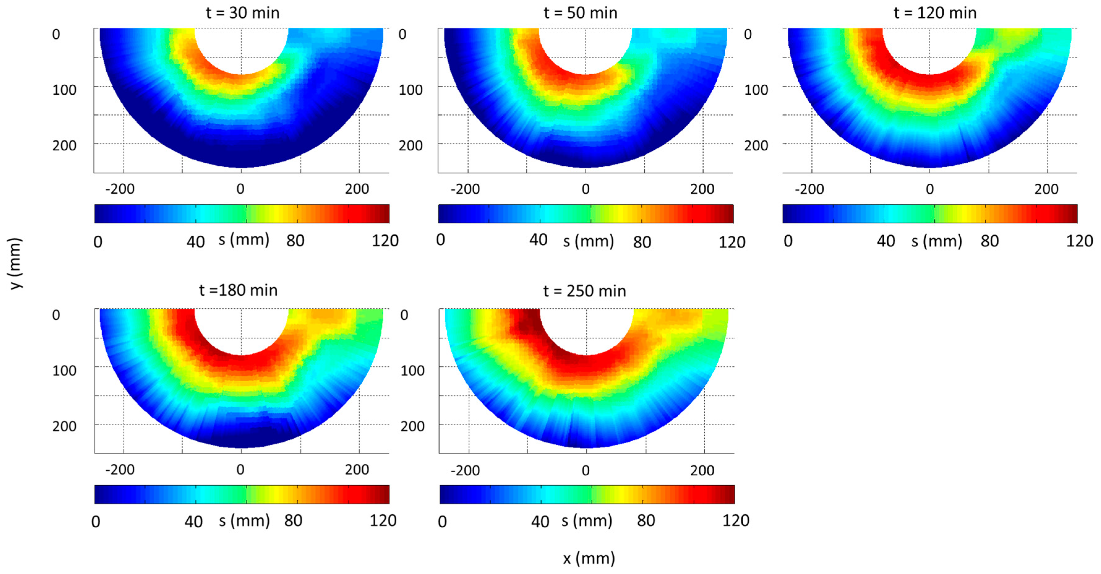
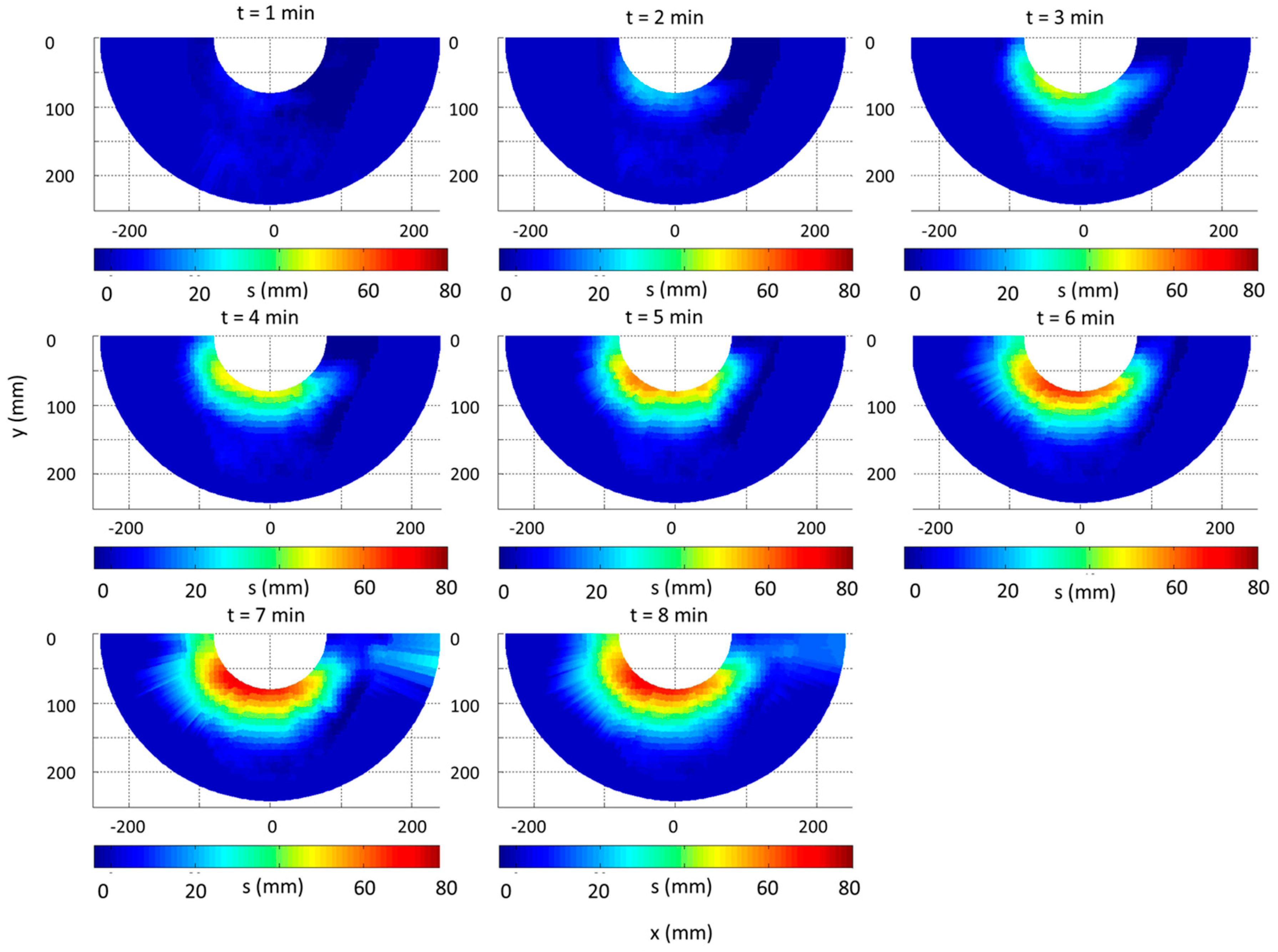
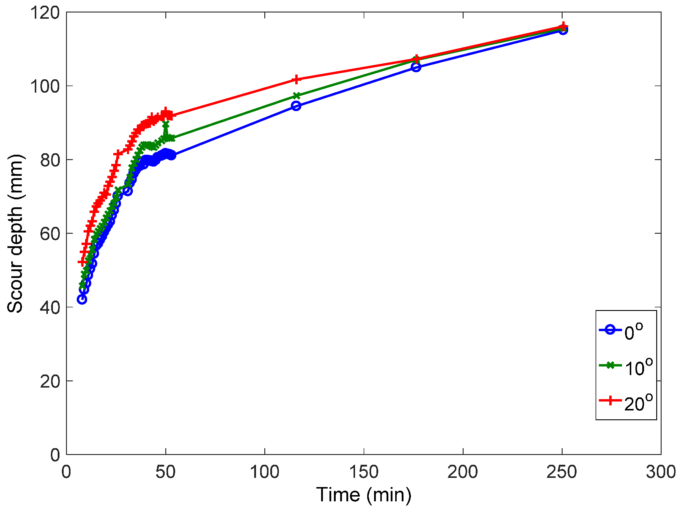
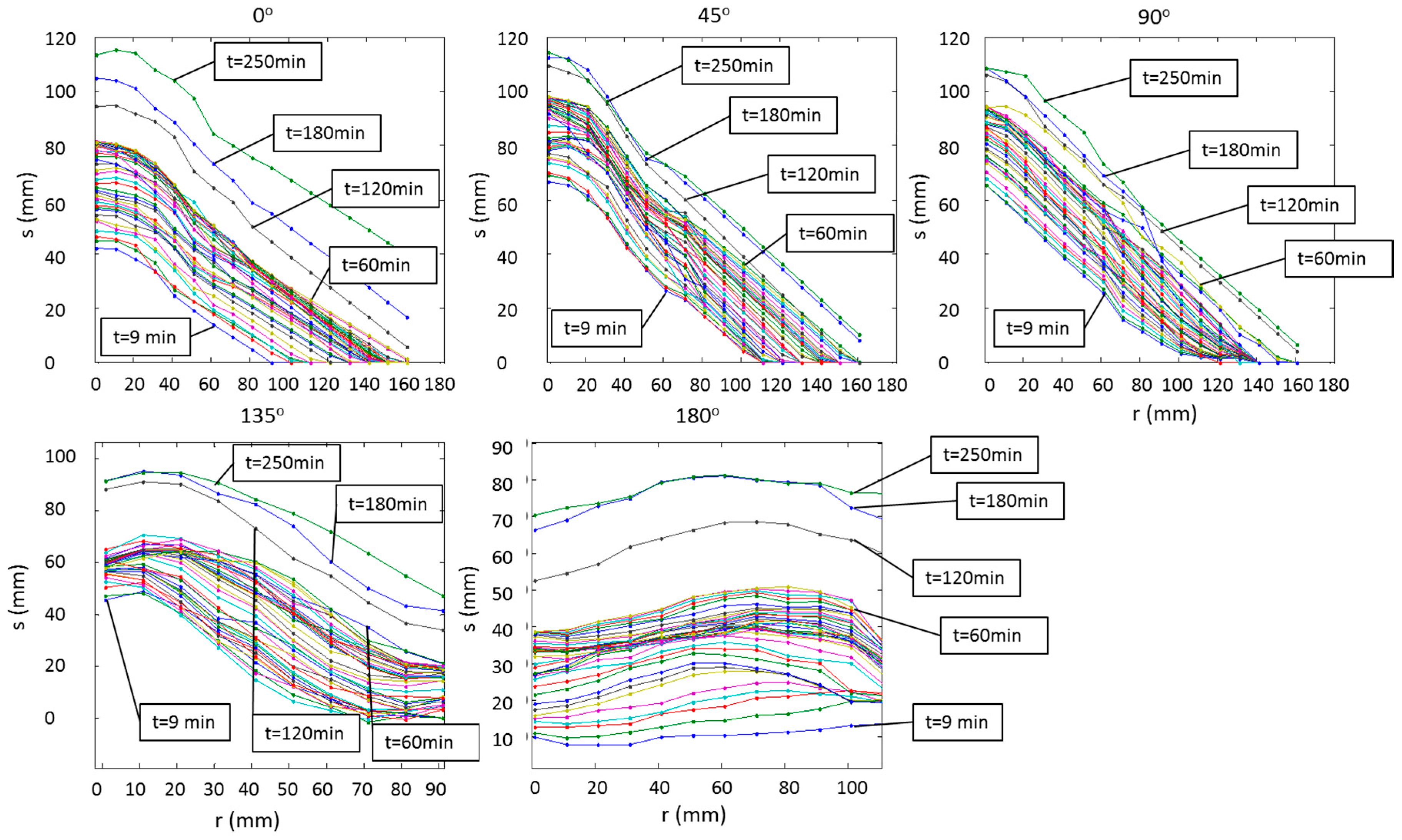
3.1. Overview of the Scour Hole Evolution

In this section series of scour depth and scour-rate maps are presented to provide an overview of the evolution of scour. The included series of contour maps provide a useful overview of the spatial and temporal characteristics of scour. Although these maps are very accurate, they can better convey qualitative rather than quantitative features of the phenomenon. A more quantitative investigation of the statistical properties of the scour evolution is included in Section 3.2. All results are presented in terms of dimensional parameters in an effort to render the trends easier to follow. Furthermore, since data obtained from a single scour experiment are described here, a dimensionless approach would not generalize the results in a meaningful way. For most of the results a cylindrical coordinate system is used (r, θ, s); where r is the radial distance from the surface of the pier; θ is the angle of the plane around the cylinder, measured from the direction of the flow; and s is the scour depth measured from the original unscoured plane bed elevation.
Figure 2 includes representations of the scour depth maps during the first 8 min of the experiment. It is shown that scour starts at planes 45°–110° from the axis of symmetry. Some small erosion is also observed at a radial distance r = 90 mm from the surface of the cylinder, at planes 60°–100°; but the maximum scour is adjacent to the cylinder surface. From the sequence of the contour maps shown in Figure 2, it is evident that the maximum depth during the first 8 min is constantly located around the 60° plane. The scour hole expands around the perimeter of the cylinder and reaches the axis of symmetry, θ = 0°, after approximately 3 min. Scour depth along the axis of symmetry remains significantly smaller compared to that at the sides for the duration of the experiment. Overall, the radial span of the scour hole increases continuously during the first 8 min, reaching a maximum value of 107 mm at the 20° plane.
The sediments that were eroded during the first 4 min are deposited in the area confined between planes 150°–180°. The height and span of the initially formed deposition area remain essentially constant during the first 4 min. Then, this small deposition of sediments is removed and scour in the wake region begins at time (t) = 6 min.
At t = 8 min, a horseshoe-shaped scour hole has already been developed around the cylinder. The slopes of the hole are steep (up to 39°) on the sides of the cylinder and very flat (less than 15°) at the wake of the cylinder. It is noted that the maximum scour depth at t = 8 min (70.8 mm) is 61% of the maximum scour depth at t = 250 min (116.2 mm).
Additional scour depth profiles are included in Figure 3. The time interval between these consecutive snapshots is longer than those in Figure 4, because the rate of scour is more moderate and milder differences are observed. From t = 9 min to t = 30 min, the most important bathymetric differences have taken place at the front (0°–20°) and the wake (130°–180°) sectors of the cylinder. During this time interval, the maximum scour depth, which is always observed between 50° and 60°, is moderately increased (from 72.5 mm to 92.8 mm). Similarly, the contour maps at t = 50 min, 120 min and 180 min, show that changes in local bathymetry are more pronounced at the sectors 0°–20° and 155°–180°. From t = 30 min to t = 180 min, the scour depth at the front of the cylinder is increasing faster (from 82.8 mm to 107.3 mm), compared to the side (from 92.8 mm to 111.2 mm). Also, during this period, the horizontal span of the scour hole is increasing uniformly around the cylinder, except for the wake region. The width of the wake region is decreasing, as a deep groove that has formed adjacent to the cylinder is expanding towards the downstream direction. From t = 180 min to t = 250 min, the bathymetric changes are very small and are characterized by the increased scour depth at the front of the cylinder and increased width of the groove adjacent to the cylinder. At t = 250 min, the maximum scour depth is marginally higher at the upstream axis of symmetry, compared to the sides of the cylinder, for the first time since the beginning of the experiment.

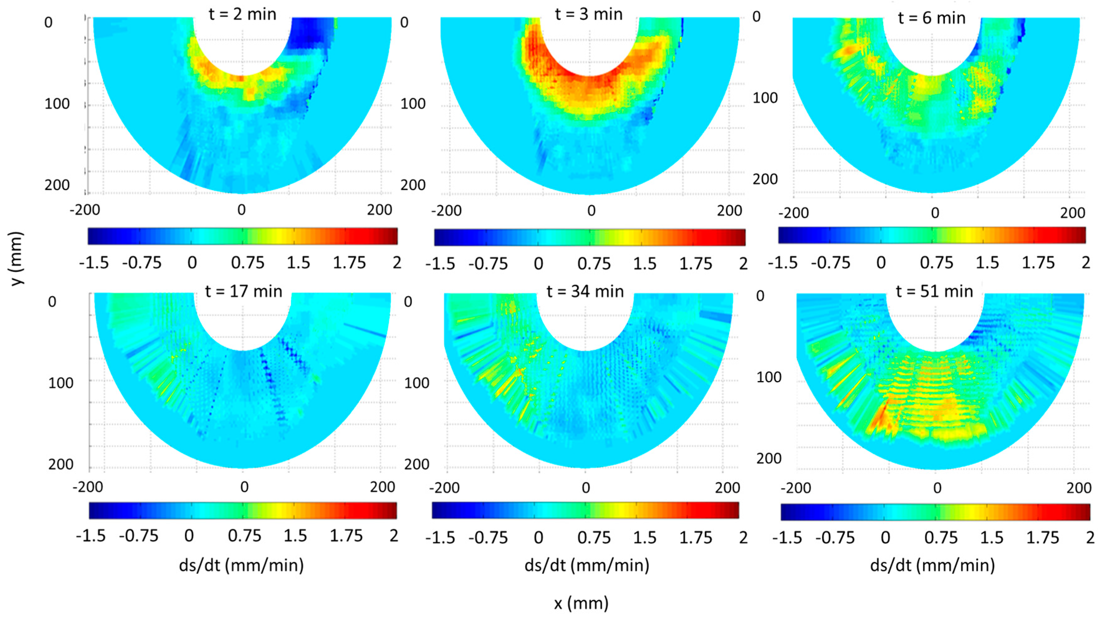
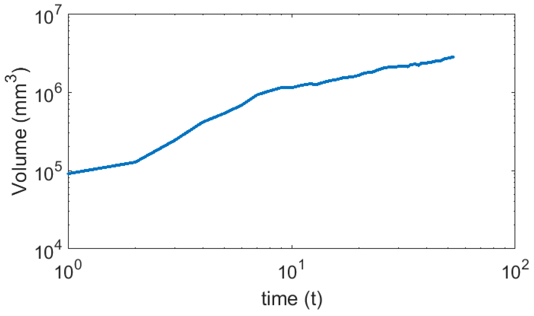
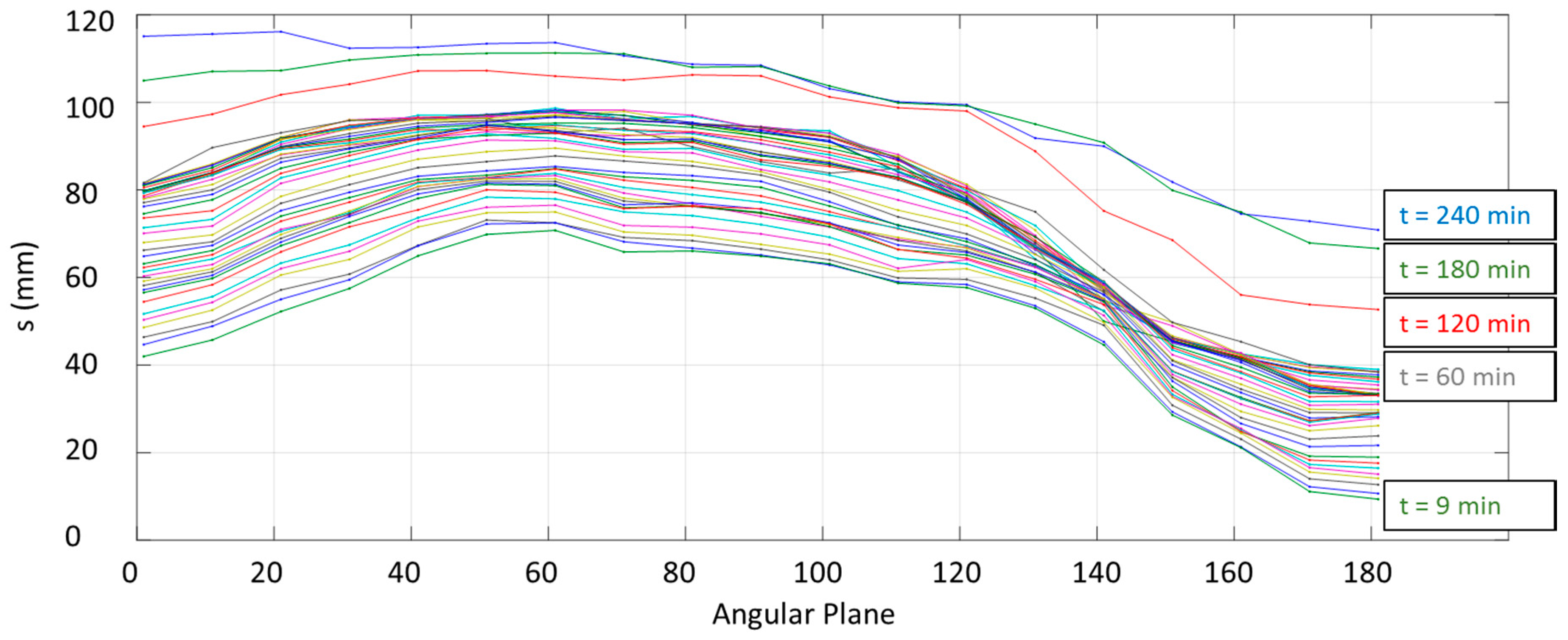
3.2. Overview of the Scour Rate Evolution and Distribution

In an effort to identify the change in the rate of scour activity with location, corresponding maps were developed (Figure 4). The rates were estimated as follows: (1) A dense cylindrical grid (18 × 20) that covers the area of the reconstructed topographies was defined at every instant (Figure 5). The radial distance between the points of the grid was 1 cm and the angular offset was 1°; (2) The scour evolution at every point of the grid was calculated; (3) The gradient of every point-wise scour evolution curve was estimated and values of rates were assigned to all the grid points, at every instant; (4) New contour maps were reconstructed from the grid with the rate values.
In Figure 4, at t = 2 min and t = 3 min, it is shown clearly that scour starts at the side of the cylinder and it is initially progressing at higher rates there. At the same instants, it is shown that scour rates at the 0° plane are very low and that sediments are deposited downstream of the cylinder immediately after the initiation of scour. At t = 6 min, the scour rates have been reduced and the maximum values are observed in patches that are not located directly adjacent to the cylinder, but coincide approximately with the location of the maximum scour depth as shown in Figure 2. Also, at this instant, scouring has already begun at the wake of the cylinder. The rate of scour in the wake region during the period of 6–8 min (not shown here) is higher compared to that observed in any other area within the scour hole.
At the contour maps after t = 8 min, it is observed that scour rates have been further decreased and their distribution does not follow any particular pattern. As an example of this random distribution, the scour rate maps at t = 17 min, 34 min and 51 min are included in Figure 4. It is shown that the maximum rates form smaller patches whose location varies in time. At some instants the scouring activity is very low at all locations (e.g., t = 17 min), and at some other instants most of the high-rate patches are accumulated at the front of the cylinder (e.g., t = 34 min), or at the side of the cylinder (e.g., t = 51 min). Overall, the most notable feature of the sequence of the scour rates is that after t = 8 min, the location, distribution and magnitude of the instantaneous rates vary significantly with time. Consequently, the distributions of scour rates averaged over longer periods (not shown here) are very low and uniform. The contrast in the evolution of the scour hole before and after t = 8 min suggests initially the presence of an organized structure whose effects subsequently disappear and, as a result, the phenomenon becomes more random.
The examination of all the series of scour rates shows that during t = 0–8 min the maximum scour rates coincide with the location of maximum scour depth. On the other hand, after t = 8 min, low duration peaks of high scour rates appear at random locations. These values reveal a very slow evolution pattern when averaged over 20 min or more.
To provide a more complete overview of the temporal evolution of scour, the volume of the excavated material of the reconstructed scour holes as a function of time is plotted in Figure 6. The temporal evolution of the volume can be accurately described by two power curves. The breakpoint between the two curves is observed at about t = 9 min. As mentioned earlier, this instant also marks the difference in the spatial distribution of the scour rates. Another important comparison between the temporal evolution of the rates and the volume is that despite the random distribution of the low duration maximum scour rate locations, the overall eroded volume, after t = 9 min, is very well described by a single power curve.
Therefore, the scour hole evolution could be divided in two phases, namely one before and one after t = 9 min. Also, there can be made a crude categorization of different areas around the cylinder. The initial and development phases, and the front, side and wake regions will be defined here to assist the presentation of the results and their discussion in the following sections. Table 1 includes the limits of the phases and the regions and some of their characteristics that will be discussed next.

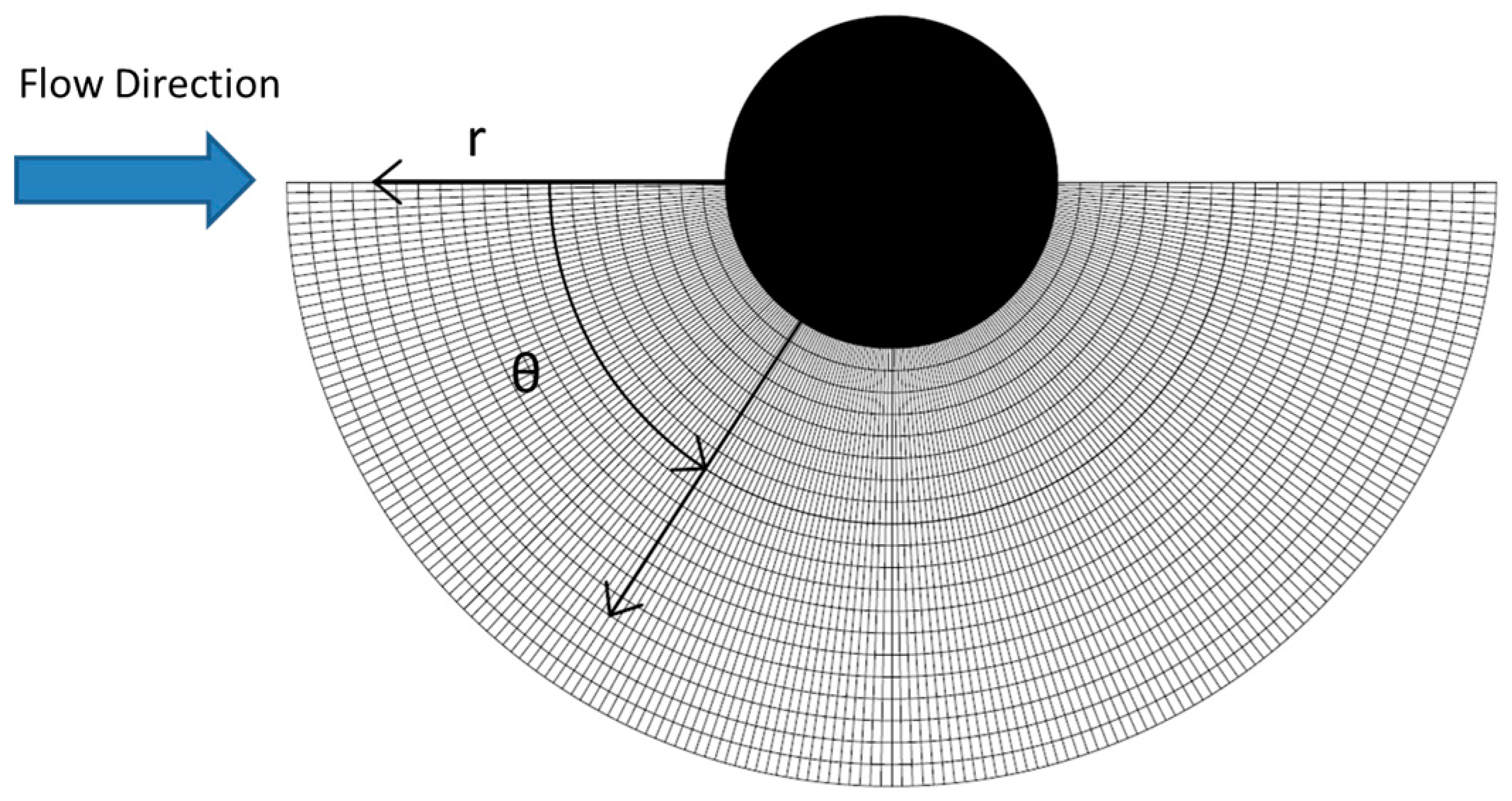
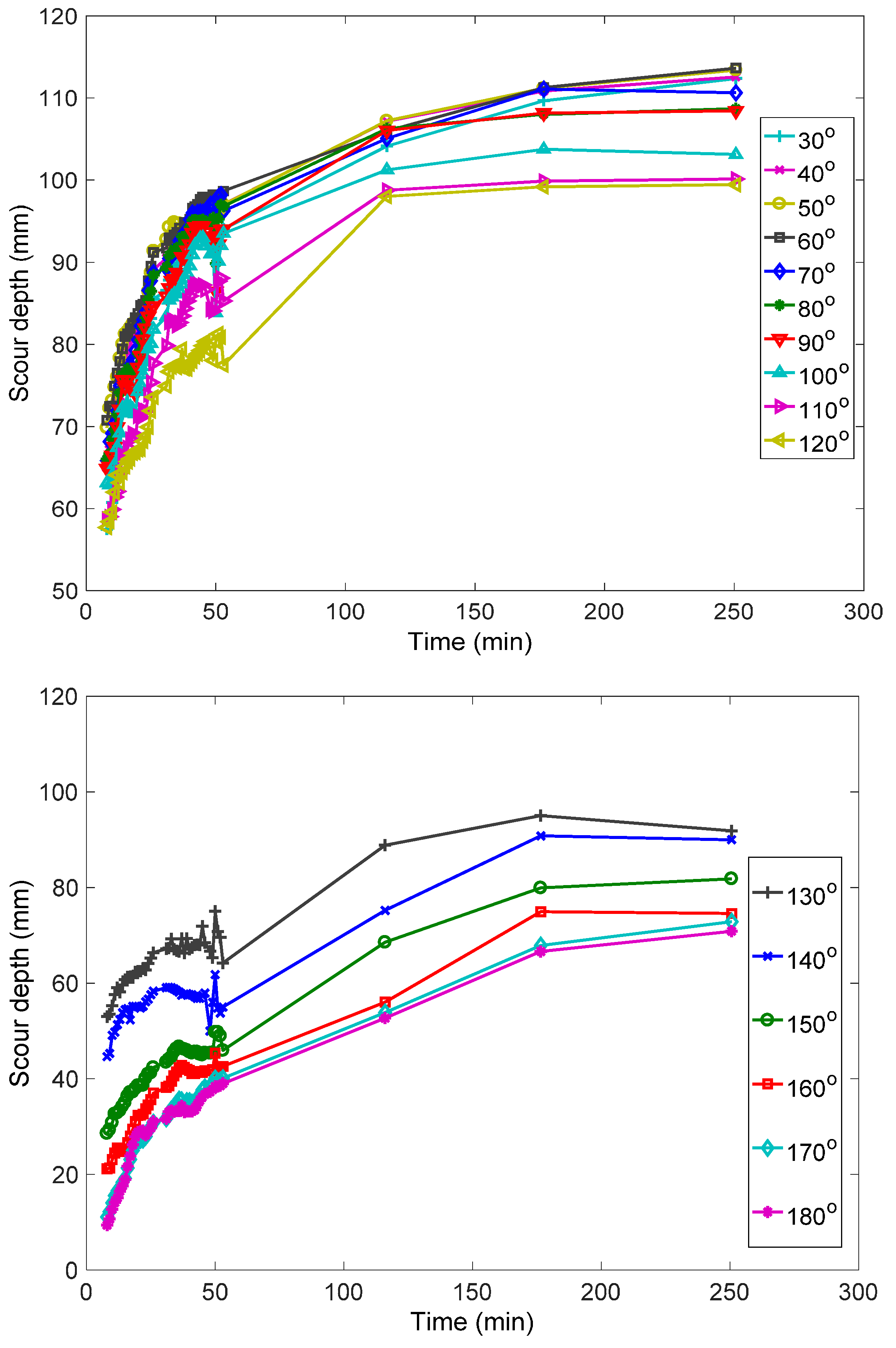
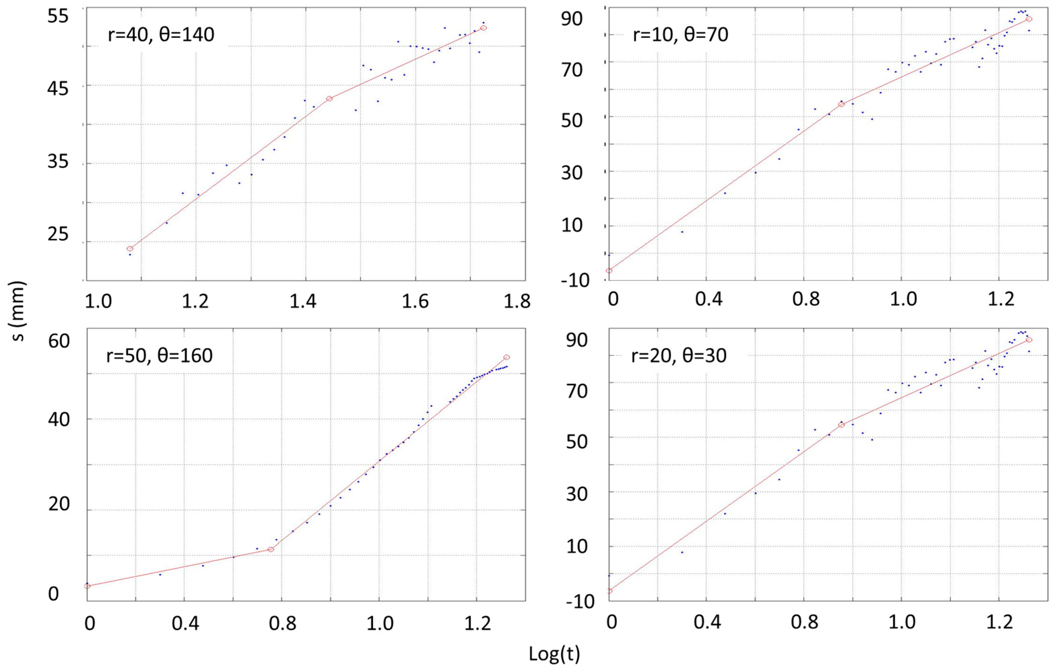
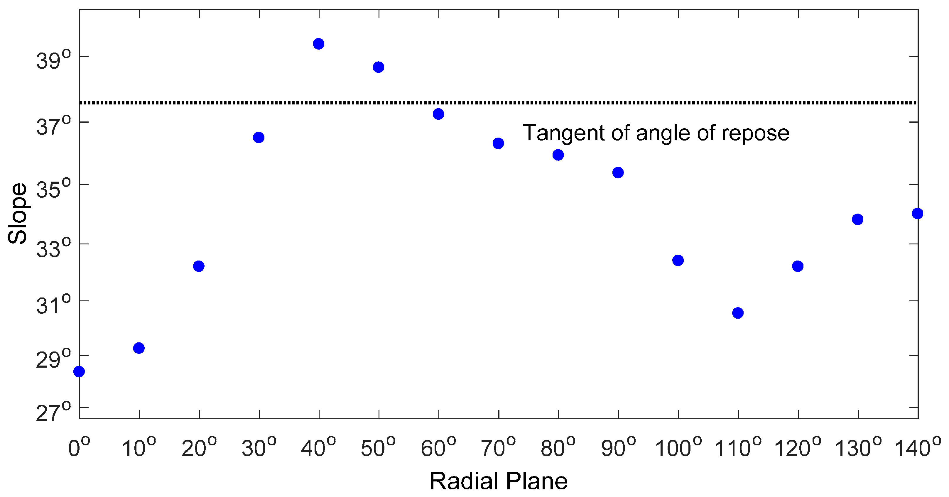
3.3. Dependence of Scour Depth on Location and Time

For the same 18 × 20 cylindrical grid a regression analysis was carried out to express scour depths as function of time. To do that, a Matlab code was written to fit logarithmic, power and polynomial functions to describe the temporal evolution of scour at all locations and evaluate the statistical justification of these functions based on the coefficient of determination (R2) and the sum of squared errors (SSE). It was found that the temporal evolution of the scour depth at every location with θ < 130° could be optimally (R2 > 0.95) described by a piecewise power function, with one breakpoint. The area of the scour hole with θ ≥ 130° was described less successfully (R2 ~ 0.7) by power functions. Table 1 shows the general form of the equations that describe scour as a function of time and Figure 7 illustrates some examples of the curve fitting results. The breakpoint that most accurately separates the two distinct scour rates was placed successfully at t = 9 min for the locations where scour started during the first 3 min of the experiment (see Figure 2). At the locations where scour started later, the breakpoint was placed at succeeding instants that varied significantly.
An additional distinction could be made for the area with θ 0° < θ ≤ 20° where the slopes of the curves after the breakpoint were consistently higher compared to the slopes of the curves at 20° < θ < 130°. This is illustrated in Figure 8, where pointwise scour is plotted against time for locations with r = 10 mm and θ varies from 0° to 180°. It is shown that after the initial phase (t ≥ 9 min) the scour rate at 0° < θ ≤ 20° is greater compared to the other plane sectors. As a result, at t = 250 min the scour depth is higher at this region. As can be observed in Figure 8, the shapes of the scour depth evolution curves for θ ≥ 130° are significantly different compared to the other planes, and they cannot be described accurately by a relatively simple function.
The second part of the morphological investigation was the regression analysis between the instantaneous scour depth and the radial distance from the cylinder (Figure 9). The most important observation in Figure 9 is that the slopes of all radial profiles within the scour hole remain relatively constant after t = 9 min. Also, the plots at planes 0° to 90° show more clearly the existence of the deeper groove that is located immediately adjacent to the cylinder and it was also observed in Figure 2 and Figure 3. The width of the groove is decreased towards the downstream direction. Despite the deepening effect of the groove, the regression analysis for the angular planes at the front and the sides of the cylinder (0° < θ < 130°), can be well approximated (R2 > 0.9) with linear curves whose slopes remain relatively constant in time but vary with θ. On the other hand, the radial profiles at θ ≥ 130° cannot be represented with linear functions of r as effectively. Instead second- or third-degree polynomials should be used to approximate the local bed topography along angular planes at the wake (Table 1).
The time-averaged slope of every radial profile, after t = 9 min was found from the instantaneous linear fits of the radial profiles (as shown in Figure 9). The results are plotted in Figure 10. It is shown that the average slopes at different angular planes vary significantly. They increase from θ = 0° to θ = 40° and then they decrease from θ = 40° to θ = 110°. Also, the time-averaged slopes at approximately 35° ≤ θ ≤ 55° are higher than the estimated angle of repose (35°).
The final part of the morphological analysis included the investigation of functional relationships between scour (s) and angular plane (θ) (Figure 11). It is shown that after t = 9 min, at r = 5 mm, s can be expressed as a sinusoidal function of θ (Table 1). Notably, the period of the sinusoidal equation that is defined in Figure 11, is similar to the period of the sinusoidal function that could be used to represent the average slope of the radial profiles in Figure 10. As a result, a sinusoidal equation between s and θ could be applied at any r. The only area that does not follow this trend is at the front face of the cylinder (θ < 20°). At the latter location, scour depth increases at higher rates, as discussed above.

4. Discussion

Based on the results summarized in Table 1, we can define two phases of temporal scour development and identify three regions that exhibit distinct spatial scour hole evolution processes. Specifically, the initial phase lasts until t = 9 min and is followed by the scour development phase that lasts until the end of the experiment (t = 250 min). Regarding the spatial discretization of the scour hole, the angular limits of each region relative to the flow direction, are: θ ≤ 20° for the front region, 20° < θ < 130° for the side region and 130° ≤ θ ≤ 180° for the wake region.

4.1. Interpretation of the Results

During the initial scour phase, scour starts and evolves at very high rates at the side region (Figure 2 and Figure 4). This is attributed to the higher bed stresses that are caused by the contraction of the streamlines as flow moves around the cylinder [10,26]. In general, the distribution of the scour rates, that remains relatively constant during the initial phase, provides a good representation of the distribution of the shear stresses whose intensity and duration are sufficiently high to induce particle entrainment [32]. Specifically, the sinusoidal distribution of the scour depth around the cylinder (Figure 7) is consistent with the results of flow measurements in previous studies. The velocity measurements of [11], over a developing scour hole, showed that the bed shear increases from the 0°-plane to the 45° plane and then it keeps decreasing continuously at the 90°, 135° and 180° radial planes. Our results show a similar trend with the maximum scour depth located at the 65° plane. Further, it is noteworthy that the slope of the scour hole in the radial direction, around the cylinder follows a similar distribution with the time-averaged shear stress and scour depth (Figure 10). Consequently, these experimental results do not support the common assumption that the slopes of the scour hole at every angular plane, except for the wake region, are equal to the angle of repose [33,34,35]. Also, the slopes at the angles 40° to 60° are higher than the angle of repose. Such steep slopes can be supported by hydrodynamic forces, potentially attributed to the presence of a horseshoe vortex within the scour hole, that partially counteract gravity. This interaction was evident from visual observations of scour. Specifically, it was observed that during the development phase sediments were sliding inside the scour hole, and were subsequently transferred downstream by the eulerlocal vortices, as has been described in several previous studies (e.g., [36,37]).
Overall, the fact that the location of maximum time-averaged erosion rates coincides with the maximum depth suggests that scour during the initial scour phase is driven by local shear stresses whose distribution in space remains constant. As a matter of fact, measurements in [5,38] have shown that the time-average shear stresses at the sides of cylinders on flat beds are up to 10 times as high as those measured in the approach flow upstream of the junction. The flat bed geometry can be representative of the initial instants of scour of an erodible bed.
Another feature of the scour hole that was observed in both bed topographies (Figure 2 and Figure 3) and the angular planes (Figure 9), is the existence of the deeper groove around the cylinder that is expanding with time. The groove has also been observed in [39,40] and it has been attributed to the existence of a corner vortex that is located at the intersection of the bed with the cylinder and rotates in the opposite (counterclockwise) direction compared to the primary horseshoe vortex [41].
At the beginning of the development phase, two important differences are observed compared to the initial phase: (1) the rate of scour at the front region is higher compared to the sides and the wake (Figure 8); and (2) the rate of scour at any location within the scour hole is reduced (Figure 7 and Figure 8). The former could be attributed to the stabilization of the core of the horseshoe vortex upstream of the cylinder, as it has also been suggested in [10,11,27]. This is further supported by the fact that the slopes of the radial profiles remain relatively constant in time (Figure 9).
The reduced scour rates, at the front and side regions, are commonly explained by the increase in the size of the horseshoe vortex that scales with the span of the scour hole [13,28,29]. As the size of the horseshoe vortex increases, its strength decreases and exerts lower shear stresses on the bed. If we associate these flow investigations with the present results, we could conclude that the stabilization of the horseshoe vortex is manifested by the breakpoint in the power plots of scour depth and volume (Figure 6, Figure 7 and Figure 8). Also, it is remarkable that the reduction of the strength of the horseshoe vortex that leads to the decreased average shear stresses and marks the end of the initial scour phase, occurs only 9 min after the beginning of the experiment.
During the development phase, the distribution of the scour rates (Figure 4) implies that scour is driven by peaks of high bed stresses with relatively high duration, randomly distributed in space, and that there is no indication of high-impulse events that act persistently at the same location. This observation resembles the findings of the numerical simulations in [8] in scour holes that were close to equilibrium. However, in the present experiment this observation is valid a few minutes after the beginning of scour. This suggests that a quasi-equilibrium state is typically reached fairly early in the scouring process, at the completion of the initial phase, especially in the front and side regions. The persistence of the quasi-equilibrium stage for the remainder of the experiment and similarity of the horseshoe vortex hydrodynamic behavior throughout this period support a consistent trend of scour development. This indicates that two temporal phases are sufficient to represent the scour hole evolution trends, in the front and side regions.
Overall, despite the seemingly random distribution of the maximum scour rates, the point-wise temporal evolution of the scour depth (at the front and the sides), (Figure 7 and Figure 8), and the volume of the eroded material (Figure 6) are well described by a power function. Also, because the slopes are constant during the development phase, it can be concluded that the horizontal span of the scour hole at every plane is proportional to the scour depth at every plane, therefore it evolves following a power function as well.
Regarding the wake region, it is shown in Figure 8 that the scour evolution follows different patterns in different locations. Also, the slopes of the radial profiles (Figure 9) within the wake region are becoming flatter towards the wake region. According to the literature, the flow components that drive the temporal evolution and the shape of the wake region are the vortices that are shed periodically downstream of the pier [4,40] and the oscillating legs of the horseshoe vortex [28,29,40]. Similar to the observations at the front and the side regions, there is not an evident imprint of the aforementioned flow components in the scour rate maps. The erosional pattern in the wake region detected through the image analysis supports the notion of a scour hole driven by instantaneous peaks of impulse.
Further, in Figure 3 it is observed that the angular span of the wake region is reduced in time, as the deep groove is expanding around the cylinder. This trend was also observed in the vorticity contour maps of [28].
Overall, it is concluded that the initial phase, despite its short duration, is critical for modelling purposes because 61% of the 4-h scour depth is developed then and because after this phase the shape of the scour hole does not undergo significant changes, thus supporting the notion of a quasi-equilibrium condition.

4.2. Evaluation of the Measurements

Although the computational algorithms and the reliability of the experimental technique have been thoroughly discussed in [30], a brief description is included here for completeness purposes. The first step of the technique involves the extraction of synchronized frames from the videos and the calibration of the cameras. The second step is the processing of the extracted frames and the establishment of stereo correspondences via cross-correlation. At the third step, stereo triangulation is carried out to derive clouds of 3D points at every instant, using the camera calibration parameters and the stereo correspondences. Finally, at the fourth step, outliers are removed and surfaces are fitted to the 3D points.
Error is generated at every step of the technique and cannot be accurately estimated via theoretical methods. Instead, the expected error of the technique was estimated by the reconstruction of objects with known dimensions and sediment beds with known elevations [30]. A long series of validation measurements showed that the accuracy of the technique (i.e., mean value of errors) is 2.31 mm and the precision (i.e., root mean square of errors) is 0.86 mm. For the experiment presented here, the error of 20-point gauge measurements had a mean value equal to 1.8 mm and RMS (root mean square) equal to 0.75 mm. Regarding the intrusiveness of the experimental technique, experimental runs with and without the presence of cameras in the water demonstrated that there is no observable effect on the scour hole dimensions. The same conclusion was drawn from visual observations of the flow during the experiment.
One of the limitations of the current results, is that some areas of the scour hole were not measured, because they were not located within the common field of view of the cameras. These areas include: (1) the largest part of the scour hole at the opposite side of the plane of symmetry; (2) small areas close to the outer edge of the scour hole, at the side region, after t = 60 min; and (3) the entire deposition area downstream of the wake region. Regarding the area across the plane of symmetry, it is common practice to assume symmetry in bridge scour experiments given the symmetric nature of the flow. Next, the occluded areas near the edge of the scour hole were reconstructed through extrapolation to better visualize the results. Due to the location (relatively far from the cylinder) and size of these areas (always less than 4 cm2) it is expected that the results and discussion presented here cannot be significantly affected. Finally, though an investigation of the characteristics of the depositional area would be very interesting, such information is not necessary for the conclusions that are drawn here.
There is ambiguity about the temporal evolution of the bed characteristics after the end of the measurements. Specifically, past studies [26,42] have identified an additional temporal phase before equilibrium. Therefore, it is possible that the new curves could be used to describe the evolution of scour or volume after the end of the presented measurements. However, the purpose of this study was not the investigation of the equilibrium conditions, but rather the temporal and spatial characteristics of the phenomenon. Based on the presented results, it is expected that further variations in the characteristics of the scour evolution, if any, would take place at significantly lower rates.
It is emphasized that the spatiotemporal characteristics of scour are expected to vary with different experimental parameters. Therefore, the purpose of this study is not to provide general rules applicable to any bridge scour simulation. However, the physical interpretation of the results and their correlation with existing flow investigations in similar setups, provide insight towards the understanding of the phenomenon. Also, the results presented here represent the most comprehensive and detailed description of the evolution of a scour hole the authors are aware of and could be used for the interpolation and/or explanation of experimental results of lower resolution or accuracy. It should be noted that previously suggested distinctions of phases or areas, in existing studies, were not defined quantitatively; rather they were mostly based on visual observations.
Finally, based on some of the most commonly used cases of bridge scour simulations [43,44], the experiment considered here is representative of clear-water conditions, with intermediately shallow flow, and uniform, non-cohesive and of intermediate degree of relative coarseness sediments in a subcritical flow. This is probably the most commonly studied case of bridge scour that can be found in the literature.

5. Conclusions

A new computer vision-based technique was employed to monitor the morphological characteristics of an evolving gravel bed at the base of a cylinder, in clear water scour conditions, with very high temporal and spatial resolution. Dynamic characteristics of the bed, such as point-wise bathymetry at various locations and slope around the cylinder and volumes of excavated material, were calculated from the measured bed topography. The evaluation of the calculated statistics led to the categorization of the scour phenomenon in two main temporal phases, namely the initial (0 min < t < 9 min) and the development (9 min < t < 250 min) phases. Also, the area of the scour hole was divided into three main regions, which are the front (0° ≤ θ ≤ 20°), the side (20° < θ < 130°) and the wake (130° ≤ θ ≤ 180°) regions. During both phases, the temporal evolution of scour at the front and the side region and the volume of the excavated material are well described by power laws. Although similar classifications have been reported in the past, this is the first time that the distinction of phases and regions of scour is based on detailed experimental data and a quantitative characterization of their limits and their spatiotemporal statistics (Table 1).
It is shown that during the brief initial phase of scour, the bed material was eroded very fast. The maximum scour rates were concentrated on the side region and their spatial distribution remained relatively constant during the initial phase. At the end of this phase, the variation of the bed’s bathymetry and radial slopes at different angles relative to the flow direction resembled the distribution of the shear stresses in that area, as has been described in past studies. Consequently, the maximum radial slopes were observed at planes 40° ≤ θ ≤ 50° and were marginally greater than the sediments’ angle of repose. It is conjectured here that the end of the initial phase and the beginning of the development phase were associated with the stabilization of the horseshoe vortex within the scour hole and resulted in important changes in the dynamic behavior of the bed. Specifically, the distribution of the maximum scour rates was characterized by small patches whose location was constantly changing in time. During the development phase scour evolved faster at the front region and the wake region, and only limited activity was observed in the side region. Remarkably, the radial slopes of the scour hole remained essentially the same during the development phase.
Overall, the experiment employed in this study represents a simple geometry that has been widely used in the past for investigations of the flow characteristics. This similarity allows for straightforward comparisons between the topography of the evolving scour hole as measured here, and the topology of the flow field obtained from previous physical or numerical models. The detailed characterization of the brief but very important initial phase is an element that is usually missing from most existing scour studies. This study contributes to the understanding of the scour phenomenon and the dynamic interaction between the flow and the evolving bed.
The dynamic morphological features that were documented here could be used to examine the validity of numerical simulations and evaluate their accuracy.

Acknowledgments

The authors would like to thank the National Science Foundation (grants EAR 0738759 and CBET-1033196) and the Research Office of the United States Army Corps of Engineers (ARO 53512-EV) for their support for this study. The first author is also grateful to the Gerondelis Foundation and the Edna Bailey Sussman Foundation.

Author Contributions

Pol Bouratsis, Panayiotis Diplas and Clinton L. Dancey conceived the experiments; Pol Bouratsis designed and performed the experiments; Pol Bouratsis analyzed the data; Panayiotis Diplas, Clinton L. Dancey and Nikolaos Apsilidis contributed to the analysis and the interpretation of the results; Pol Bouratsis, Panayiotis Diplas and Clinton L. Dancey wrote the paper.

Conflicts of Interest

The authors declare no conflicts of interest.

References

  1. Johnson, P.A.; Jones, J.S. Merging laboratory and field data in bridge scour. J. Hydraul. Eng.-ASCE 1993, 119, 1176–1181. [Google Scholar] [CrossRef]
  2. Sheppard, D.M.; Demir, H.; Melville, B.W. Scour at Wide Piers and Long Skewed Piers; National Research Council (U.S.), Transportation Research Board, National Cooperative Highway Research Program, American Association of State Highway and Transportation Officials, and Federal Highway Administration: Washington, DC, USA, 2011. [Google Scholar]
  3. Baker, C.J. The Turbulent Horseshoe Vortex. J. Wind. Eng. Ind. Aerod. 1980, 6, 9–23. [Google Scholar] [CrossRef]
  4. Dargahi, B. The Turbulent-Flow Field around a Circular Cylinder. Exp. Fluids 1989, 8, 1–12. [Google Scholar] [CrossRef]
  5. Devenport, W.J.; Simpson, R.L. Time-dependent and time-averaged turbulence structure near the nose of a wing body junction. J. Fluid Mech. 1990, 210, 23–55. [Google Scholar] [CrossRef]
  6. Apsilidis, N.; Diplas, P.; Dancey, C.L.; Bouratsis, P. Time-resolved flow dynamics and Reynolds number effects at a wall-cylinder junction. J. Fluid Mech. 2015, 776, 475–511. [Google Scholar] [CrossRef]
  7. Paik, J.; Sotiropoulos, F. Numerical simulation of strongly swirling turbulent flows through an abrupt expansion. Int. J. Heat Fluid Flow 2010, 31, 390–400. [Google Scholar] [CrossRef]
  8. Escauriaza, C.; Sotiropoulos, F. Initial stages of erosion and bed form development in a turbulent flow around a cylindrical pier. J. Geophys. Res.-Earth 2011, 116. [Google Scholar] [CrossRef]
  9. Koken, M.; Constantinescu, G. An investigation of the dynamics of coherent structures in a turbulent channel flow with a vertical sidewall obstruction. Phys. Fluids 2009, 21, 085104. [Google Scholar] [CrossRef]
  10. Istiarto, I.; Graf, W.H. Experiments on flow around a cylinder in a scoured channel bed. Int. J. Sediment Res. 2001, 16, 431–444. [Google Scholar]
  11. Dey, S.; Raikar, R.V. Characteristics of horseshoe vortex in developing scour holes at piers. J. Hydraul. Eng.-ASCE 2007, 133, 399–413. [Google Scholar] [CrossRef]
  12. Debnath, K.; Manik, M.K.; Mazmder, B.S. Turbulence statistics of flow over scoured cohesive sediment bed around circular cylinder. Adv. Water Resour. 2012, 41, 18–28. [Google Scholar] [CrossRef]
  13. Kumar, A.; Kothyari, U.C.; Raju, K.G.R. Flow structure and scour around circular compound bridge piers—A review. J. Hydro-Environ. Res. 2012, 6, 251–265. [Google Scholar] [CrossRef]
  14. Beheshti, A.A.; Ataie-Ashtiani, B. Scour hole influence on turbulent flow field around complex bridge piers. Flow Turbul. Combust. 2016, 97, 451–474. [Google Scholar] [CrossRef]
  15. Melville, B.W.; Chiew, Y.M. Time scale for local scour at bridge piers. J. Hydraul. Eng.-ASCE 1999, 125, 59–65. [Google Scholar] [CrossRef]
  16. Kothyari, U.C.; Hager, W.H.; Oliveto, G. Generalized approach for clear-water scour at bridge foundation elements. J. Hydraul. Eng.-ASCE 2007, 133, 1229–1240. [Google Scholar] [CrossRef]
  17. Simarro, G.; Teixeira, L.; Cardoso, A.H. Closure to “Flow Intensity Parameter in Pier Scour Experiments” by Gonzalo Simarro, Luis Teixeira, and Antonio H. Cardoso. J. Hydraul. Eng.-ASCE 2009, 135, 155. [Google Scholar] [CrossRef]
  18. Link, O.; Castillo, C.; Pizarro, A.; Rojas, A.; Ettmer, B.; Escauriaza, C.; Manfreda, S. A model of bridge pier scour during flood waves. J. Hydraul. Res. 2016. [Google Scholar] [CrossRef]
  19. Oliveto, G.; Hager, W.H. Temporal evolution of clear-water pier and abutment scour. J. Hydraul. Eng.-ASCE 2002, 128, 811–820. [Google Scholar] [CrossRef]
  20. Lu, J.Y.; Shi, Z.Z.; Hong, J.H.; Lee, J.J.; Raikar, R.V. Temporal Variation of Scour Depth at Nonuniform Cylindrical Piers. J. Hydraul. Eng.-ASCE 2011, 137, 45–56. [Google Scholar] [CrossRef]
  21. Umeda, S.; Yamazaki, T.; Ishida, H. Time evolution of scour and deposition around a cylindrical pier in steady flow. In Proceedings of the International Conference on Scour and Erosion, Tokyo, Japan, 5–7 November 2008; pp. 140–146.
  22. Dodaro, G.; Tafarojnoruz, A.; Sciortino, G.; Adduce, C.; Calomino, F.; Gaudio, R. Modified Einstein sediment transport to simulate the local scour evolution downstream a rigid bed. J. Hydraul. Eng.-ASCE 2016, 142. [Google Scholar] [CrossRef]
  23. Radice, A.; Porta, G.; Franzetti, S. Analysis of the time-averaged properties of sediment motion in a local scour process. Water Resour. Res. 2009, 45, 12. [Google Scholar] [CrossRef]
  24. Radice, A.; Tran, C.K. Study of sediment motion in scour hole of a circular pier. J. Hydraul. Res. 2012, 50, 44–51. [Google Scholar] [CrossRef]
  25. Link, O.; Pfleger, F.; Zanke, U. Characteristics of developing scour-holes at a sand-embedded cylinder. Int. J. Sediment Res. 2008, 23, 258–266. [Google Scholar] [CrossRef]
  26. Dargahi, B. Controlling Mechanism of Local Scouring. J. Hydraul. Eng.-ASCE 1990, 116, 1197–1214. [Google Scholar] [CrossRef]
  27. Kirkil, G.; Constantinescu, G. Flow and turbulence structure around an in-stream rectangular cylinder with scour hole. Water Resour. Res. 2010, 46, W11549. [Google Scholar] [CrossRef]
  28. Escauriaza, C.; Sotiropoulos, F. Reynolds Number Effects on the Coherent Dynamics of the Turbulent Horseshoe Vortex System. Flow Turbul. Combust. 2011, 86, 231–262. [Google Scholar] [CrossRef]
  29. Khosronejad, A.; Kang, S.; Sotiropoulos, F. Experimental and computational investigation of local scour around bridge piers. Adv. Water Resour. 2012, 37, 73–85. [Google Scholar] [CrossRef]
  30. Bouratsis, P.; Diplas, P.; Dancey, C.L.; Apsilidis, N. High-resolution 3-D monitoring of evolving sediment beds. Water Resour. Res. 2013, 49, 977–992. [Google Scholar] [CrossRef]
  31. Sabersky, R.H.; Acosta, A.J.; Hauptmann, E.G. Fluid Flow: A First Course in Fluid Mechanics, 3rd ed.; Collier Macmillan: New York, NY, USA, 1989. [Google Scholar]
  32. Diplas, P.; Dancey, C.L.; Celik, A.O.; Valyrakis, M.; Greer, K.; Akar, T. The role of impulse on the initiation of particle movement under turbulent flow conditions. Science 2008, 322, 717–720. [Google Scholar] [CrossRef] [PubMed]
  33. Mia, F.; Nago, H. Design method of time-dependent local scour at circular bridge pier. J. Hydraul. Eng.-ASCE 2003, 129, 420–427. [Google Scholar] [CrossRef]
  34. Yanmaz, A.M.; Kose, O. A semi-empirical model for clear-water scour evolution at bridge abutments. J. Hydraul. Res. 2011, 47, 110–118. [Google Scholar]
  35. Guo, J. Semi-analytical model for temporal clear-water scour at prototype piers. J. Hydraul. Res. 2014, 52, 366–374. [Google Scholar] [CrossRef]
  36. Dey, S. Clear Water Scour around Circular Bridge Piers: A Model; Department of Civil Engineering, Indian Institute of Technology: Kharagpur, India, 1991. [Google Scholar]
  37. Euler, T.; Herget, J. Controls on local scour and deposition induced by obstacles in fluvial environments. Catena 2012, 91, 35–46. [Google Scholar] [CrossRef]
  38. Roulund, A.; Sumer, B.M.; Fredsoe, J.; Michelsen, J. Numerical and experimental investigation of flow and scour around a circular pile. J. Fluid Mech. 2005, 534, 351–401. [Google Scholar] [CrossRef]
  39. Breusers, H.N.C.; Raudkivi, A.J. Scouring; International Association for Hydraulic Research: Rotterdam, The Netherlands, 1991. [Google Scholar]
  40. Kirkil, G.; Constantinescu, G.; Ettema, R. Detached Eddy Simulation Investigation of Turbulence at a Circular Pier with Scour Hole. J. Hydraul. Eng.-ASCE 2009, 135, 888–901. [Google Scholar] [CrossRef]
  41. Apsilidis, N.; Diplas, P.; Dancey, C.L.; Bouratsis, P. Effects of wall roughness on turbulent junction flow characteristics. Ex Fluid 2016, 57. [Google Scholar] [CrossRef]
  42. Melville, B.W.; Raudkivi, A.J. Flow characteristics in local scour at bridge piers. J. Hydraul. Res. 1997, 15, 373–380. [Google Scholar] [CrossRef]
  43. Melville, B. Pier and Abutment Scour: Integrated Approach. J. Hydraul. Eng.-ASCE 1997, 123, 125–136. [Google Scholar] [CrossRef]
  44. Sheppard, D.M.; Melville, B.; Demir, H. Evaluation of Existing Equations for Local Scour at Bridge Piers. J. Hydraul. Eng.-ASCE 2014, 140, 14–23. [Google Scholar] [CrossRef]
Figure 1. (a) View of the hydraulic flume; (b) View of the cameras recording the bed during the experiment.
Water 09 00227 g001
Figure 2. Scour depth (s) contour maps during the first 8 min of the experiments. Flow direction is from left to right. t: time.
Water 09 00227 g002
Figure 3. Scour depth contour maps at various instants. Flow direction is from left to right.
Water 09 00227 g003
Figure 4. Instantaneous scour rate distributions.
Water 09 00227 g004
Figure 5. The cylindrical grid that was used for the statistical analysis of the scour hole’s morphology. r: radial distance from the surface of the pier; θ: angle of the plane around the cylinder.
Water 09 00227 g005
Figure 6. Temporal evolution of the eroded volume.
Water 09 00227 g006
Figure 7. Examples of the piecewise curve fitting for the temporal functions of scour.
Water 09 00227 g007
Figure 8. Temporal evolution of scour at locations with r = 10 mm and θ ranging from 0° to 180°.
Water 09 00227 g008aWater 09 00227 g008b
Figure 9. Scour depth against radial distance from the surface of the cylinder, for various instants after t = 9 min, in 5 angular planes, around the cylinder.
Water 09 00227 g009
Figure 10. Average slope of radial profiles during the development phase.
Water 09 00227 g010
Figure 11. Average slope of radial profiles, at r = 5 mm, at the front and the sides of (or around) the cylinder during the development phase.
Water 09 00227 g011
Table 1. Quantitative characteristics of the various phases and regions. Parameters ci are constants used in the derived equations.
Initial Scour PhaseDevelopment Scour Phase
(0 min ≤ t < 9 min)(9 min ≤ t ≤ 250 min)
FrontSideWakeFrontSideWake
(0 ≤ θ ≤ 20)(20 < θ < 130)(130 ≤ θ < 180)(0 ≤ θ ≤ 20)(20 < θ < 130)(130 ≤ θ < 180)
Terminal scour depth (mm)46.070.823.9116.2114.280.5
Location of max scour depth (θ, r)(20, 30)(60, 30)(175, 180)(0, 20)(60, 5)(175, 100)
Terminal eroded volume (mm3)1.14 × 1064.76 × 106
Scour (s) vs. Time (t)s = tc1s = tc1 + c2Undefineds = tc1s = tc1 + c2Undefined
Scour (s) vs. Angular Plane (θ)Undefineds = c3sin(c4θ) + c5
Scour (s) vs. radial distance (r)s = c5r + c6s = c7r3 + c8r2 + c9r + c10s = c5r + c6s = c7r3 + c8r2 + c9r + c10
Eroded Volume (V) vs. Time (t)V = tc11V = tc11 + c12
Slope of the angular profile (Z) vs. Angular Plane (θ)UndefinedZ = c13sin(c14θ) + c15Undefined

