
Effects of Pore-Scale Geometry and Wettability on Two-Phase Relative Permeabilities within Elementary Cells


1
Dipartimento di Ingegneria Civile e Ambientale (DICA), Politecnico di Milano, Piazza Leonardo da Vinci 32, 20133 Milano, Italy
2
Department of Hydrology and Atmospheric Sciences, Tucson, AZ 85721, USA
*
Author to whom correspondence should be addressed.
Water 2017, 9(4), 252; https://doi.org/10.3390/w9040252
Submission received: 26 January 2017
/
Revised: 23 March 2017
/
Accepted: 27 March 2017
/
Published: 5 April 2017
(This article belongs to the Special Issue Water and Solute Transport in Vadose Zone)
Abstract
:We study the relative role of the complex pore space geometry and wettability of the solid matrix on the quantification of relative permeabilities of elementary cells of porous media. These constitute a key element upon which upscaling frameworks are typically grounded. In our study we focus on state immiscible two-phase flow taking place at the scale of elementary cells. Pressure-driven two-phase flow following simultaneous co-current injection of water and oil is numerically solved for a suite of regular and stochastically generated two-dimensional explicit elementary cells with fixed porosity and sharing main topological/morphological features. We show that the relative permeabilities of the randomly generated elementary cells are significantly influenced by the formation of preferential percolation paths, called principal pathways, giving rise to a strongly nonuniform distribution of fluid fluxes. These pathways are a result of the spatially variable resistance that the random pore structures exert on the fluid. The overall effect on relative permeabilities of the diverse organization of principal pathways, as driven by a given random realization at the scale of the elementary cell, is significantly larger than that of the wettability of the host rock. In contrast to what can be observed for the random cells analyzed, the relative permeabilities of regular cells display a clear trend with contact angle at the investigated scale.
1. Introduction
Multi-phase flows within natural and engineered porous structures are ubiquitous [1,2]. In the context of groundwater quality and subsurface energy management and exploitation, the migration of NAPLs (Non-Aqueous Phase Liquids) through the vadose zone and multi-phase dynamics in oil bearing formations and their feedback with overlying fresh groundwater bodies constitute an example of the interest in the issues associated with our understanding of such flow settings. Despite recent progress in studying these processes, knowledge of them is still far from being complete. Multi-phase flows are characterized by a multiscale nature, being distributed over a multiplicity of scales ranging from pore- to continuum-scales. This has suggested the development and application of upscaling frameworks to derive macroscopic models able to capture key features of processes occurring at the pore-scale. Upscaled models are typically formulated in terms of effective medium properties that are evaluated on the basis of micro-scale characteristics. The latter are commonly evaluated within elementary (or unit) cells (e.g., [3,4,5,6,7]).
Upscaling procedures based on homogenization via multiple scale expansion [4,8] or volume averaging techniques [9,10] have been proposed to analyze immiscible continuous or dispersed (e.g., [6]) two-phase flow in porous media as well as non reactive (e.g., [3,5]) and reactive (e.g., [11] and references therein) transport processes. The upscaling of immiscible two-phase flow has also been proposed through the thermodynamically constrained averaging theory by Gray and Miller [12]. Auriault [4] and Whitaker [9,10] derived effective models for two-phase immiscible fluid flow that include terms representing the effect of viscous coupling between flowing phases. When the latter phenomenon is negligible or the same pressure gradient is applied to both fluids, these models reduce to the traditional Darcy-Buckingham equation, i.e., , with subscript α indicating fluid phase, and , , , and K respectively being Darcy velocity, dynamic viscosity, pressure gradient across fluid phase α, and intrinsic permeability of the medium. Here, indicates the relative permeability of fluid phase α, lumps all complexities of the interfacial fluid dynamics behavior and strongly depends on the pore-scale features. Experimental (e.g., [13,14]) and numerical (e.g., [15,16,17]) pore-scale studies focus on the way is influenced by the viscosity ratio between the two fluids, the capillary number, medium wettability and initial configuration of the fluids in the system. Contact angles, which are associated with medium wettability, are recognized as key parameters in controlling macroscopic features of multiphase flow, such as fluid arrangement in the pore space and relative permeabilities. Nowadays there is a strong potential for their direct evaluation through advanced imaging techniques ([18,19] and reference therein). This element is also evidenced in Trojer et al. [20], wherein the displacement pattern of two migrating fluid phases is analyzed for diverse contact angles in a radial Hele-Shaw cell packed with glass beads. It has also been suggested that the micro-scale structure of the void space might play a critical controlling role on relative permeabilities and on the spatial arrangement of the flowing phases [21] at diverse spatial scales of interest. In this context, Liu et al. [22] presented a numerical study of an unsteady displacement problem for a two-dimensional setting, in which the solid phase is modeled through a set of non-overlapping circles associated with a random distribution of their diameter and location of their center, representing disaggregated porous media. Random realizations of pore-scale topological features have been employed in the context of pore network modeling of immiscible two-phase flows by Jiang et al. [23]. These authors investigated the effects on flow properties of random microscopic rock features, highlighting the key role of the connectivity function.
The choice of the geometrical features of the pore space of elementary cells significantly impacts effective coefficients evaluated with upscaling procedures (e.g., [24,25,26]). Icardi et al. [27] pointed out the need to include uncertainty in pore-scale physics to be used in upscaling models.
The assessment of the joint role that the uncertain geometry of an elementary cell and medium wettability have on relative permeabilities is still an open and challenging problem. Here we tackle this issue and study the role of wettability and pore-scale structure of realistic randomly generated and regular elementary cells in fluid phase distribution and relative permeabilities characterizing steady state immiscible two-phase flows. We do so through a set of numerical simulations of two-phase fluid flow performed in a diffusive-interface framework within two-dimensional explicit pore spaces representing elementary cells which can be employed for upscaling studies.
2. Materials and Methods
2.1. Generation of Regular and Random Elementary Cells
We consider water and oil as immiscible displacing fluids, i.e., the fluid phase α = w (water) or o (oil). We explore a suite of twelve two-dimensional elementary cells: (i) three media associated with an explicit regular structure of the pore space (hereafter termed as settings HDη, with η = a, b, c); and (ii) nine stochastically generated explicit pore spaces (hereafter termed Ei, with i = 1, …, 9). Each case is characterized by the same macro-scale characteristics, i.e., size of the medium along x-, Lx = 3.98 × 10⁻³ m, and y-, Ly = 3.45 × 10⁻³ m directions (see Figure 1), and connected porosity, n ≈ 0.5.
Systems in which solid elements are regularly distributed in space, as in HDη, are commonly employed in upscaling studies of flow and transport processes [6,7]. The elementary cell HDa (see Figure 1a) is composed of circular grains of diameter Dg = 0.48 mm with throat diameter Dt = 0.11 mm. Dg is chosen to guarantee that the Specific Surface Area (SSA) of the regular geometries is equal to the average SSA of the nine random samples, while Dt controls the sample porosity. Systems HDb and HDc are characterized by elliptical and square solid elements with round corners, respectively (see Figure 1b,c).
The random elementary cells we consider are generated on a rectangular lattice of size Lx/2 and Ly/2 using the procedure implemented in Hyman et al. [28] and in Siena et al. [29], to which we refer for additional details about the generation techniques and code as well as the associated generation parameters. The synthetic generation approach employed has been shown to produce realistic pore spaces and pore space geometric observables such as porosity and SSA to be controlled through the appropriate tuning of generation parameters [30]. Virtual pore spaces generated using this method were used to investigate the influence of (a) porosity on transport properties [28]; (b) porosity and mean hydraulic radius on single-phase fluid flow permeability [31]; (c) pore wall geometry and network topology on local mixing [32]; and (d) pore size distributions on fluid velocity statistics [29], as well as to assess the way in which statistics of porosity and SSA are affected by scale [33,34].
The generated samples are then mirrored along the x- and y-directions to obtain the periodic heterogeneous pore structures required by upscaling approaches. Figure 1d–l depicts the nine heterogeneous elementary cells we consider. As listed in Table 1, the connected porosity of all analyzed samples is virtually the same and equal to the value set for the regular media (≈0.5). Table 1 also lists values of sample SSA. This quantity contributes to control transport dynamics and does vary considerably in all of the cases.
2.2. Pore Space Spatial Correlation
All random cells are characterized by the same structure of the pore space spatial correlation. The latter has been described by analyzing the directional variograms ( being spatial separation distance rescaled by the domain size Li with i = x, y) of the indicator function, I (I = 1 in the solid matrix and I = 0 otherwise), of the pore space. These variograms are interpreted through a Maximum Likelihood (ML) approach (details not shown) via a spherical model, i.e., for 0 ≤ ≤ and for > , , and respectively representing variogram sill and range (rescaled by Li). ML estimates of , , and , , for all random samples are listed in Table 1. The degree of correlation of the void spaces, as quantified by , does not vary significantly with direction (indicating isotropy of the correlation structure of the pore spaces) and across samples (i.e., the spatial correlation structure of void spaces and solid matrix is statistically equivalent for all geometries). The variogram sill is fairly constant for all geometries and close to the theoretical value .
2.3. Topological/Morphological Analysis of the Elementary Cells
Both regular and random elementary cells are associated with comparable topological and morphological features. These characteristics are not controlled by the generation algorithm we employ and can be assessed a posteriori. We investigate the structure of the pore spaces within a pore-network framework using the maximal ball algorithm described in Dong and Blunt [35]. Each pore is associated with a coordination number, Cn, representing the number of pores connected to the pore under consideration. Figure 2 depicts the relative frequency of Cn evaluated in the nine random samples. The patterns of the shapes of the distributions associated with different geometries indicate that the systems share similar topological characteristics. Table 2 lists the total number of pores, Npores, the average coordination number, , and the ratio computed for the regular structures (HDa, HDb, HDc) and for each of the random samples considered. The ratio , which is a measure of the global connectivity of the pore network, is constant for the three regular domains HDη and varies weakly among the nine stochastic pore spaces, the coefficient of variation of being about 20%. Note that, on average and in seven of nine cases, the heterogeneous structures appear to be more connected than the regular ones.
To further characterize the morphology and the topology of the pore structures, we evaluate the Minkowski functionals by relying on the algorithm proposed by Mantz et al. [36]. These functionals are geometric measures defined for binary structures (see for details [37,38,39]). In a two-dimensional setting they correspond to the area of the solid phase (M0), the boundary length between solid and fluid (M1) and the Euler number (M2). While M0 and M1 are morphological measures, M2 is a topological metric describing connectivity. The latter is calculated by counting the number of isolated objects from which the number of redundant connections is subtracted and is negative for well connected structures and positive otherwise. The results listed in Table 2 show that all of the considered structures are well connected. Note also that, according to M2, the regular structure HDc appears to be characterized by the lowest connectivity.
2.4. Single Phase Flow Simulations
All flow simulations are performed using the finite element software COMSOL Multiphysics [40] by relying on a triangular element mesh. A body force of magnitude ΔP/Lx, with ΔP = 39.8 Pa, acts along the x-direction (from left to right in Figure 1). This magnitude has been selected to be comparable to a body force produced by the gravity (ρ|g|, where ρ = 1000 kg m−3 is the fluid density and |g| is the absolute value of gravitational acceleration).
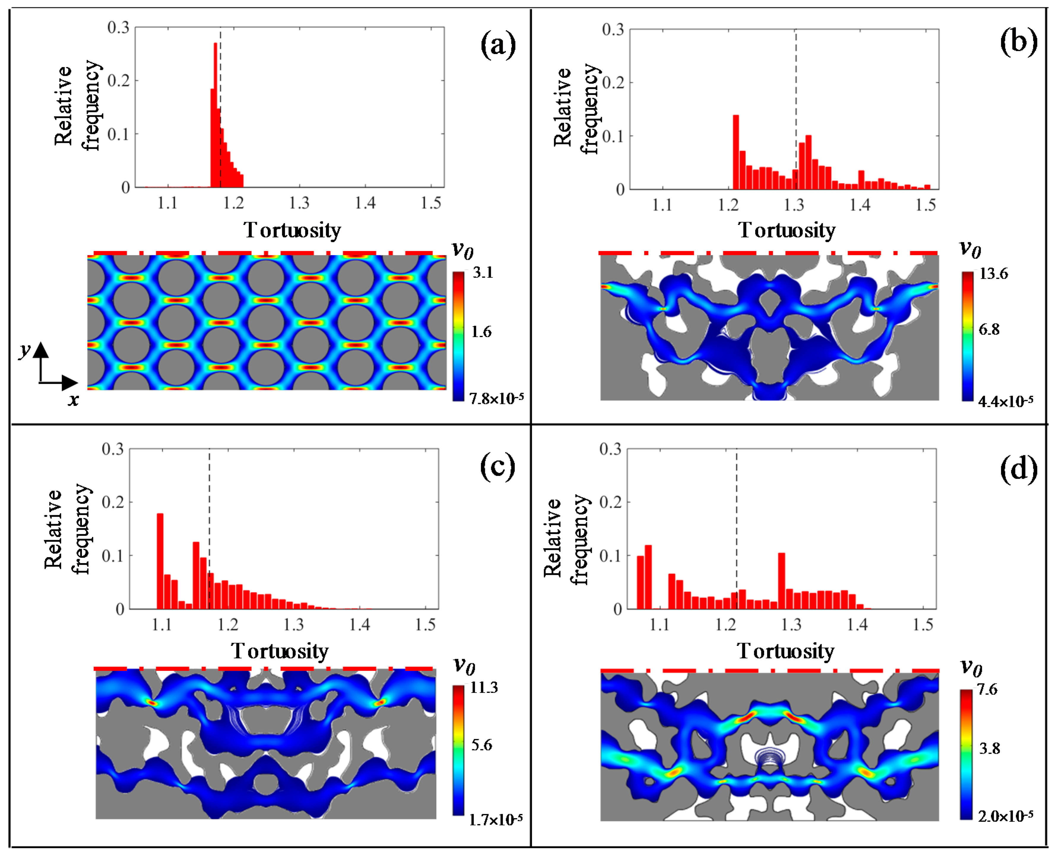
We start by solving the steady state single phase fluid problem to evaluate the intrinsic permeability , where the flow rate, Q, is obtained by integration of the steady state fluid velocity component along the y-axis at the system outlet (i.e., at x = Lx). The values of K associated with each scenario are listed in Table 1. These vary significantly across all elementary cells (either regular or random), the coefficient of variation of K for the random media being about 50%. The degree of heterogeneity of each cell is further quantified in terms of tortuosity values. We do so by considering the trajectories of N tracer particles which are released uniformly across the domain inlet (at x = 0) and advective displacement of which is tracked through the fluid domain. The tortuosity of a particle trajectory i is computed as , li being the trajectory length. Particles reaching stagnation regions are removed from the analysis, which then considers NP particles percolating through the medium. Relying on N = 5000 particles enabled us to obtain stable basic statistics of (details not shown). Depending on test case, 0.46 ≤ NP/N ≤ 0.98, as listed in Table 3. Figure 3 depicts the histogram of tortuosity, , for HDa and three selected random elementary cells. The mean, variance, skewness, and kurtosis of , are listed in Table 3. The tortuosity of HDη (η = a, b, c) varies over a narrow range of values and its histogram is characterized by a single peak. Otherwise, histograms of obtained in the randomly heterogeneous geometries exhibit a multimodal behavior and are characterized by an appreciable range of variability within and across samples (see Table 3 and Figure 3). This behavior is related to the complex spatial distribution of the void spaces characterizing the heterogeneous samples.
Colorized images of particle trajectories are depicted in Figure 3. Particles migrating in the randomly heterogeneous media tend to focus within areas of high velocity, forming trajectory bundles termed principal pathways [28]. The multimodal distribution of tortuosity for the heterogeneous cases can be related to the grouping of particle trajectories along principal pathways during percolation through the media. The emergence of these features is an intrinsic characteristic of the flow field taking place in such intricate pore structures, as opposed to what can be observed in regular pore spaces, where flow is spatially distributed according to a mostly uniform pattern. Note the occurrence of pore space regions that are not visited by particles during the time frame of the simulation (white regions in Figure 3). These observed behaviors will affect the results of our two-phase flow simulations, the ensuing fluid distribution in the pore space and the magnitude of relative permeabilities as a function of fluid saturation as discussed in Section 3.
2.5. Two-Phase Flow Simulations
Two-phase flow within the elementary cells is solved through a diffusive-interface formulation which simulates the evolution of the fluid/fluid interface within an energy based framework [41,42]. Within this approach the interface between the two phases is approximated through a small but finite transition region inside which the two components are mixed. The thickness of this region is controlled by a capillary length scale parameter, ε [41,42]. This methodology has been applied to describe steady state two-phase flows and displacement processes in porous media by Ahmadlouydarab et al. [17] and Amiri and Hamouda [43,44]. It requires the joint solution of the Cahn-Hilliard (1) and Navier-Stokes (2) equations
Here φ is the phase variable (φ = 1 in water and φ = −1 in oil), and v, p, m, and G respectively indicate fluid velocity vector, pressure, the Chan-Hilliard mobility constant and the chemical potential of the system. The latter arises from the variation of the system free energy with respect to φ and is defined as , λ being the mixing free energy density that arises from the molecular interaction between the two phases inside the transition region [41].
At equilibrium for a planar fluid/fluid interface the ratio λ/ε is proportional to the interfacial tension, , as [42,43], the quantity in (2) being the diffusive-interface representation of . Fluid density, ρ, and viscosity, μ, are defined as the average between the corresponding values associated with each fluid phase weighted by their volume fraction as with = ρ, μ. The fourth-order Chan-Hilliard Equation (1) is decomposed in two second-order equations through the auxiliary function ψ, i.e.,
Computations are therefore performed using the set of four independent variables {v, p, φ, ψ}. Bi-periodic boundary conditions are applied to the external sides of the domain for all variables of the system. The following boundary conditions are employed at the solid-fluid boundaries
with n being the unit normal vector pointing from the fluid to the solid. For the purpose of the present study we assume no slip condition on the solid matrix, ensured by the first condition of (4). The contact line motion is then due solely to Chan-Hilliard diffusion. Zero flux through the solid matrix is imposed via the second of (4), while the third of (4) corresponds to the diffuse-interface formulation of the contact angle, θ.
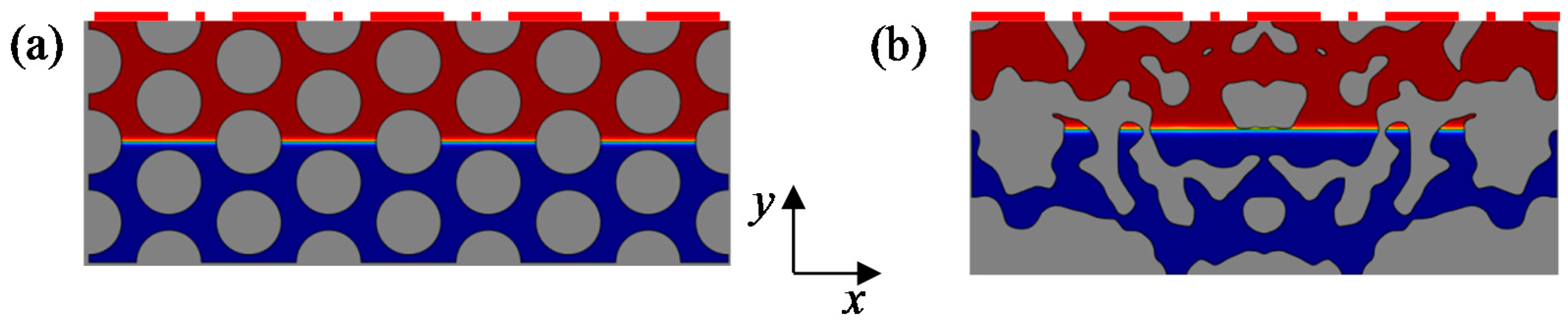
In our settings the oil phase is considered to reside initially in the central part of the system according to a given saturation, So, as exemplified in Figure 4 for HDa and E4 with So = 0.5. The initial configuration of the two phases has been selected considering that one of the assumptions underlying upscaling of two-phase flow is that the volume occupied by each fluid is connected [4]. One or both phases start flowing in the system under the action of the constant driving force until steady state conditions are reached and the resulting equilibrium configuration of the water-oil interface is observed. During the simulation the saturation of the two fluids is controlled by the bi-periodic boundary conditions applied to the external sides of the domain.
In typical experimental conditions the flow rate of the two fluid phases is imposed at the domain inlet and the pressure gradient, , between inlet and outlet is measured (see, e.g., Tallakstad et al. [14]). One can note that under these conditions the steady-state regime is commonly not identified in terms of a static equilibrium configuration of the water-oil interface and is considered to be attained in an average sense when the values of appear to fluctuate around a constant value.
Benchmarking of the numerical approach has been performed through comparison against the two-phase Poiseuille flow (details not shown). A key issue is the proper selection of the Chan-Hilliard model parameters, i.e., the capillary width, ε, and the mobility constant m [45,46] as well as the grid size h. The capillary width is associated with the Cahn number, , for the definition of which we select the pore throat of HDa as the characteristic length scale. The transition region (and therefore the associated Cn) needs to be very small to capture the physics of the two-phase flow problem [41,42]. The convergence of the numerical results with variations of h, ε and m has been verified for all settings (details not shown). On these bases and according to Amiri and Hamouda [42], we set a maximum value of h equal to 2 ε and m = ε2.
The simulations are performed by considering = 0.001 Pa s and = 0.002 Pa s (i.e., a viscosity ratio = 2), water and oil density equal to 1000 kg m−3, and interfacial tension = 0.04 N m−1, these values being representative of a typical oil/water system at reservoir condition [43,47]. Medium wettability is defined through the contact angle, θ, measured with respect to the water fluid phase. We set θ = 90°, 60° and 120° to mimic neutral wet (NW), water wet (WW) and oil wet (OW) systems, respectively. The distribution of pore-scale velocities is then computed for diverse values of So.
The magnitude of the imposed body force (the same used in single-phase simulations, Section 2.4) controls the flow rate of the two phases at steady-state and the capillary number = ( being the largest velocity of phase α along the x-direction).
We note that the largest value of the capillary number, is observed for the oil phase, and its magnitude is of the order of 10−4. This number represents the ratio of viscous to capillary forces, and the value we employ can be considered representative of standard oil/water systems at reservoir condition [44]. Albeit of interest, the study of the influence of diverse values of the capillary number (e.g., [14]) on relative permeability curves is outside the scope of the present contribution.
3. Results and Discussion
3.1. Equilibrium Two-Phase Distribution Patterns
Figure 5 depicts patterns of equilibrium (steady state) spatial distributions of the two fluid phases and streamlines in HDa and in three selected heterogeneous elementary cells for θ = 90° and So ≈ 0.5 (the actual values of So at steady state are listed in the caption of Figure 5). Pore space geometry significantly affects the steady state distribution of the interface between the two fluids and the flow field characteristics. The pattern of the flow fields in the random elementary cells is characterized by several regions not contributing to the total flow rate (clearly identifiable in Figure 5). For this degree of oil saturation both phases percolate in HDa (see Figure 5a) and in the heterogeneous samples E4 (Figure 5c) and E8 (Figure 5d), the water phase being blocked in sample E1 (Figure 5b). This behavior is related to the complex topology of the investigated geometries within which the two fluids are displaced and experience spatially variable resistances that are differently distributed depending on the realization analyzed. The percolation of the two fluids is strongly linked to (a) the number of inlet/outlet openings from which a fluid can be injected into (or exit from) each sample and (b) the distribution of principal pathways within the samples. The two fluids may flow simultaneously in cells characterized by more than one inlet and multiple principal pathways favoring the occurrence of several distinct percolation paths in the system (see Figure 3c,d). One or both fluids are immobile (at steady state) when the medium has only one inlet and/or one principal pathway (see Figure 3b). The emergence of the general patterns observed in Figure 5 has been found for all wettability values analyzed (see Figure 6).
3.2. Relative Permeabilities
The flow rate of the α phase, Qα, for a given oil saturation is computed by integrating the steady state fluid velocities along the portion of the outlet boundary through which the α phase flows. Normalization of Qα by the total flow rate computed when the medium is fully saturated by the α phase leads to an estimate of the relative permeability, Krα. We further note that the solution of closure equations associated with effective models [4,8,9,10] and leading to the evaluation of a full relative permeability tensor which includes the coupling phenomenon, is equivalent to the solution of (1)–(4), where flow is sustained by an imposed body force acting on both fluids at steady state conditions.
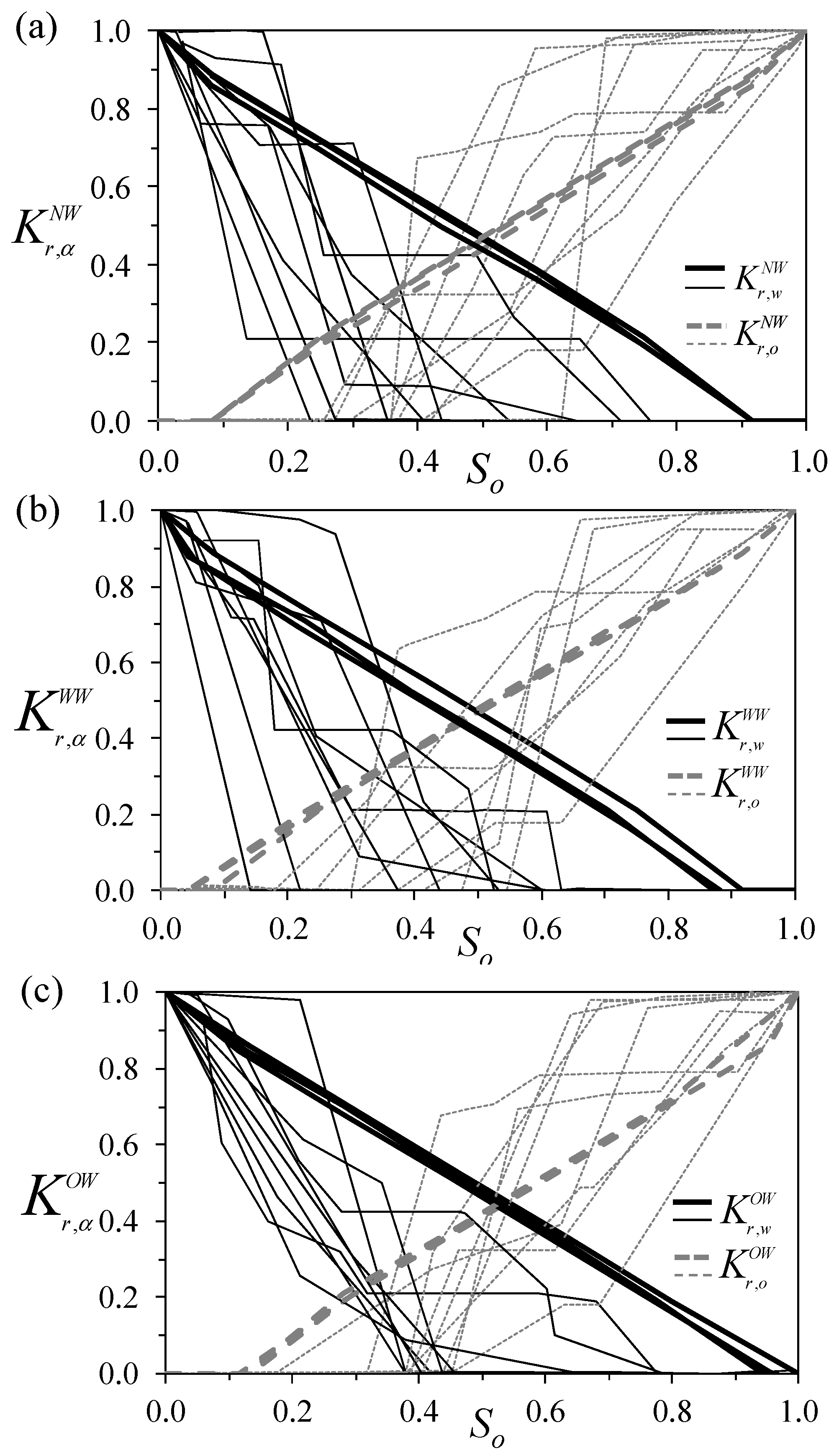
Relative permeabilities, , versus oil saturation are depicted in Figure 7 in regular media and in three selected heterogeneous elementary cells under diverse wettability conditions (here the superscript X = NW, WW and OW). It can be observed that in the regular media varies almost linearly with So for all wettability conditions analyzed (see Figure 7a–c). The simultaneous flow of both phases is observed for a wide range of saturations. Otherwise, the relative permeability values for a given saturation level consistently display a clear trend with contact angle. In this case the oil permeability under water wet conditions is higher than that corresponding to neutral or oil wet settings, the opposite behavior being documented for relative permeabilities of water. The relative permeabilities in the randomly heterogeneous cells are strongly influenced by the pore structure configuration (see Figure 7d–f) and vary in a highly non-linear fashion with fluid saturation. For instance, water relative permeability, , remains constant for all wettability values when 0.4 ≤ So ≤ 0.6, as in the case depicted in Figure 7e. This behavior is markedly controlled by the number of principal pathways and by the distribution of the two phases in the heterogeneous domains. The resulting fluid configuration could have a significant feedback with the occurrence of regions (Figure 5c) which do not contribute to water mass transport and could be linked to the number of inlet/outlet openings from which a fluid can be injected into (or exit from) a given sample. To further explore this point, we analyze the sample probability distributions (PDFs) of the horizontal component of the velocity field, uα (α = o, w, respectively for oil and water phase) normalized by the mean velocity of the corresponding phase. Results of these investigations are summarized in the Appendix A. It can be seen from these results that sample PDFs are not affected by saturation values for the homogeneous domains analyzed. For heterogeneous geometries the peak and the positive tail of the sample PDF of oil (or water) velocities tend to be respectively higher and longer with increasing saturation of the corresponding phase (i.e., So or Sw). This behavior is related to the observation that heterogeneous domains are characterized by the occurrence of regions with very limited contribution to oil/water mass transport.
Contrary to what is observed in the regular systems, the wettability conditions of a given random medium do not affect systematically the relative permeabilities of soil and water, the variability of which is mostly driven by the underlying random pore space configuration. This behavior is associated with the topological complexity of the heterogeneous cells, which shadows the influence of the contact angle on the final distribution pattern of the two fluid phases.
The role of the random pore-size distribution patterns on is further emphasized in Figure 8a where the curves evaluated for the regular settings and for the random samples are juxtaposed. The corresponding results for water and oil wet conditions are depicted in Figure 8b,c respectively. Comparison of Figure 7 and Figure 8 allows the dominant effect of random pore space geometry of the elementary cells to be recognized, as opposed to the impact of wettability on relative permeabilities. This is clearly evidenced by considering that the relative permeability values in Figure 8 are characterized by a significantly higher spread than that is evidenced in Figure 7 for a given saturation level. On the other hand, it is noted that the relative permeabilities associated with the three diverse regular settings analyzed can be barely distinguishable for a given wettability value.
Water relative permeability is generally smaller in the heterogeneous cells we analyze than in the HDη setting. This behavior is a consequence of the occurrence of regions where virtually no flow is observed for the water phase in Ei. The location of principal pathways within the medium in relation to the spatial pattern of fluid injection along the inlet section has a remarkable controlling role in the relative magnitude of oil and water relative permeabilities observed for the heterogeneous settings Ei as opposed to the regular pore distribution, where no distinct principal pathways are observed. For example, the relative permeability of oil for heterogeneous systems is always larger than that associated with the regular pore space patterns in cases where the segment along which oil injection takes place corresponds to the location of the principal pathways (e.g., samples E1, and E4; Figure 3b,c), the opposite behavior emerging when oil is injected through portions of the inlet that are not associated with principal pathways (e.g., sample E8; Figure 3d). We note that our work does not address the question of the existence or of the relevance of a representative scale for the assessment of the relative permeability curves of natural porous materials. Our findings are framed in the context of upscaling studies based on, e.g., volume averaging [48] or homogenization [49], wherein one relies on the solution of pore-scale physics at a scale that is much smaller than that of an investigated porous system.
In such a framework, results obtained at the micro-scale are used to evaluate macroscopic parameters (in our case relative permeabilities) which are intended to characterize a continuum-scale description of the system. When conditions of the applicability of these approaches are warranted, our results can then potentially be transferred to characterize larger scale systems.
The geometry of the pore space at the scale of the elementary cell is typically uncertain and this aspect impacts the quantification of macroscopic quantities such as relative permeabilities. Our results therefore support the need for considering such uncertainties when dealing with characterization of relative permeabilities based on upscaling frameworks.
3.3. Qualitative Comparison of the Numerical Results against Experimental Data
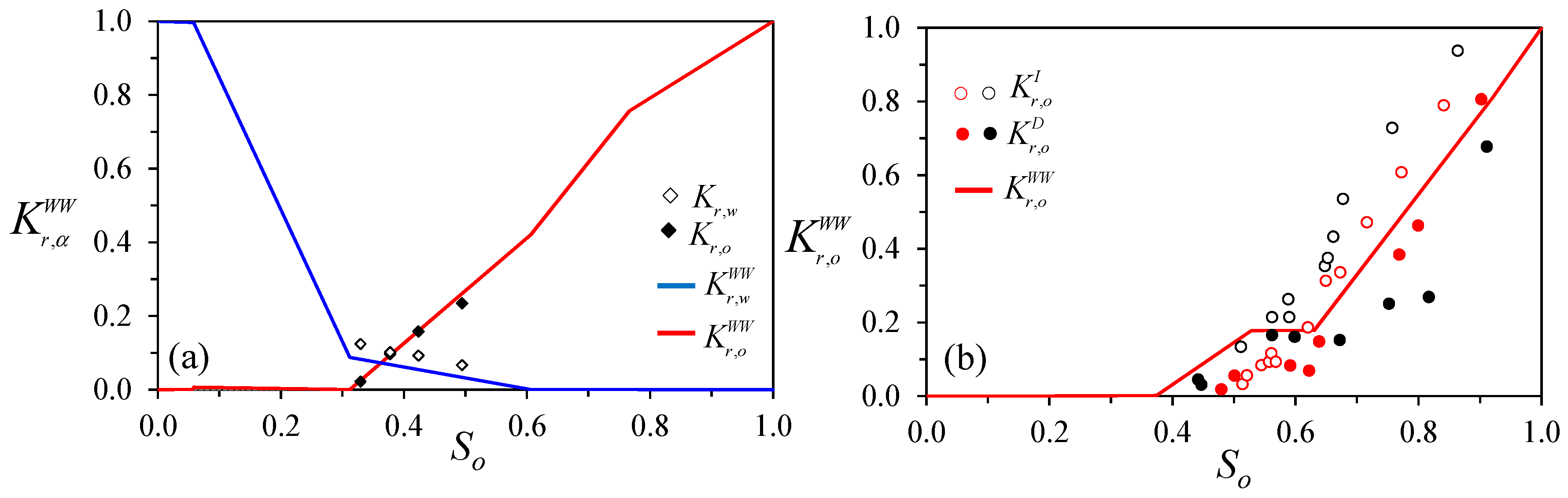
Finally, we provide a preliminary assessment of the ability of our generated pore structures to provide relative permeability curves which can be considered compatible/consistent with those arising from experimental observations. We do so by performing a qualitative comparison of our simulation results against experimental data collected within two-dimensional micromodels of porous media [13,50] under steady state conditions.
These authors analyze steady state two-phase flows at diverse capillary numbers and using diverse fluid pairs by way of two-dimensional micromodels forming a connected system of pores and throats. We collected a set of data from this study, which appears to be amenable to a qualitative comparison against our numerical results obtained under water wet conditions. The physicochemical properties of the fluids used in the experiments and in our computational analyses are listed in Table 4.
Figure 9a,b juxtapose the selected numerical results depicted in Figure 8b (curves) and the relative permeability values estimated in the considered experimental studies (symbols). Note that the experimental and numerical analyses have been performed under different conditions, e.g., in terms of the physicochemical properties of the fluids employed (see Table 4). It can be seen that the results associated with our random elementary cells are qualitatively consistent with the behavior displayed by the available relative permeability information. In this sense, it can be recognized that our relative permeability results for the random geometries display features that can be observed also in the experimental studies, namely: (a) the lack of connectivity of the oil phase for values of So smaller than a given threshold; and (b) relative permeability curves that vary in a highly non-linear fashion with fluid saturation.
When viewed also in this context, the results of our analysis are promising and suggest the worth of further systematic studies on the assessment of the way the uncertain geometry of elementary cells propagates to the macroscale description of porous media constructed through such systems.
4. Conclusions
We illustrate the role of complex micro-scale pore geometry and wettability on oil and water relative permeabilities within elementary cells under immiscible two-phase flow conditions. Two types of micro-scale elementary cells, characterized by comparable macro-scale properties and topological and morphological features, have been considered: (a) regular samples, constructed starting from a solid element of fixed geometry which is then distributed in the domain according to a regular pattern, and (b) random geometries, which share similarities with the complex pore structure of natural rocks. In the regular elementary cells, the two phases are well connected for several oil/water saturation values. This leads to relative permeabilities which vary (approximately) linearly with phase saturation and exhibit a clear trend with contact angle. In the random elementary cells, the relative permeability curves vary in a highly non-linear fashion with fluid saturation due to the occurrence of stagnant flow regions.
The key driver for the variability of relative permeability curves is the random geometry of the pore space of the elementary cell. This is clearly evidenced by our results (see Figure 7 and Figure 8), indicating that the relative permeability values associated with random pore spaces (for a given wettability) are characterized by a markedly higher spread than their counterparts related to diverse wettabilities (for a given random pore space). As our knowledge of the details of pore space structure and wettability is always incomplete, our findings: (a) have an impact on the assessment of the uncertainty associated with the quantification of relative permeabilities of porous materials stemming from the use of upscaling techniques which are based on the solution of closure equations formulated on elementary cells; and (b) suggest the need to perform systematic upscaling studies in a stochastic context to propagate the effects of uncertain pore space geometries to a probabilistic description of relative permeability at the continuum scale.
All data used in the paper will be retained by the authors for at least five years after publication and will be available to the readers upon request.
Acknowledgments
Funding from MIUR (Italian ministry of Education, University and Research, Water JPI, WaterWorks 2014, Project: WE-NEED-Water NEEDs, availability, quality and sustainability) and from the European Union’s Horizon 2020 Research and Innovation programme (Project Furthering the knowledge Base for Reducing the Environmental Footprint of Shale Gas Development FRACRISK, Grant Agreement No. 640979) is acknowledged.
Author Contributions
Emanuela Bianchi Janetti, Monica Riva and Alberto Guadagnini contributed to the setup of the methodology and to the design of the numerical simulations; Emanuela Bianchi Janetti performed the numerical simulations; and Emanuela Bianchi Janetti, Monica Riva and Alberto Guadagnini analyzed the results and contributed to the writing of the paper.
Conflicts of Interest
The authors declare no conflict of interest.
Appendix A. Probability Distribution of Velocity Fields
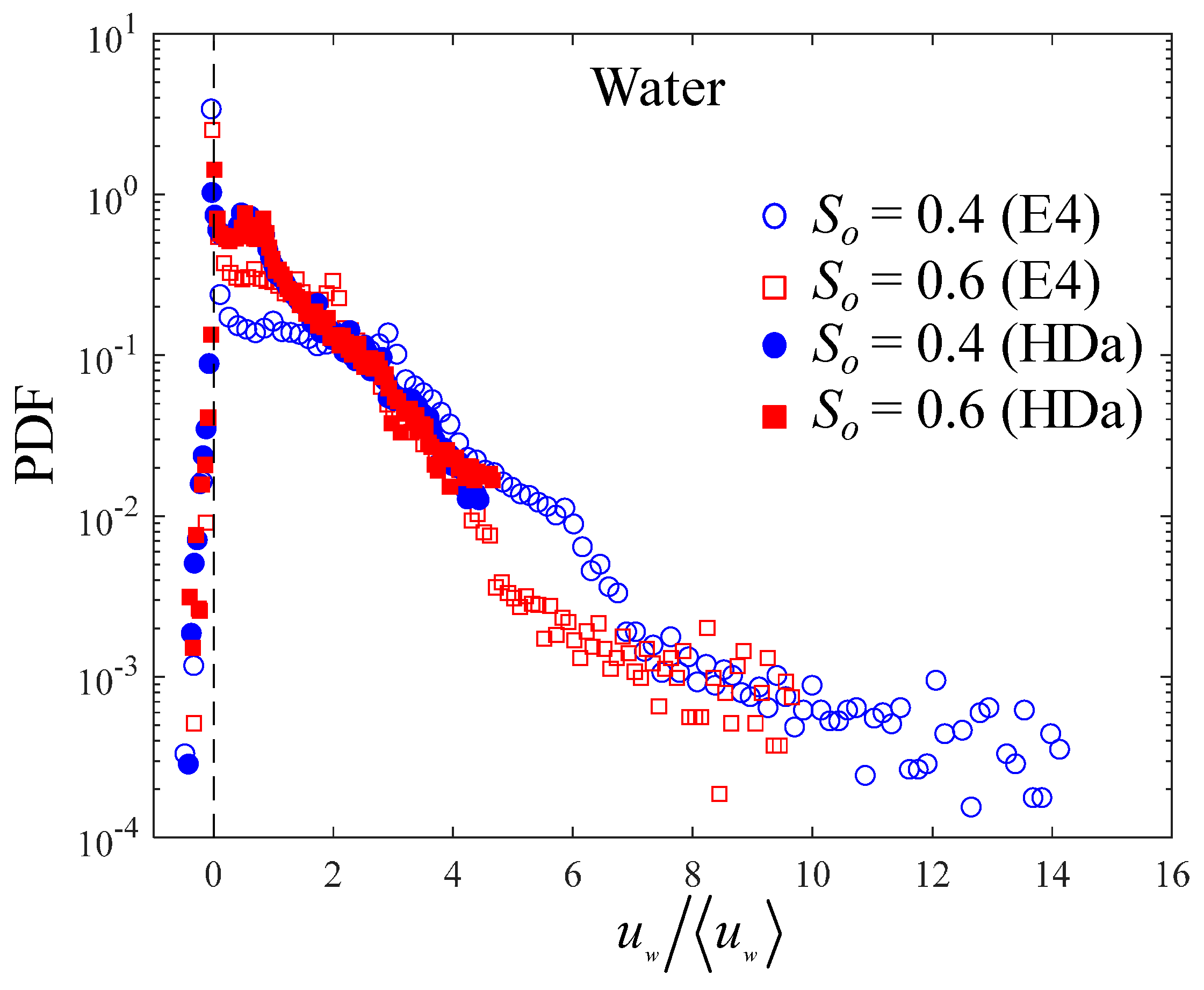
We explore the PDFs of the horizontal component of the velocity field, uα (α = o or w for oil and water phase, respectively). We compare homogeneous and heterogeneous domains considering neutral-wet conditions and diverse saturation values. Figure A1 depicts sample PDFs of , as the mean of uo over the domain occupied by the oil phase. Full and empty symbols respectively are associated with sample HDa and E4. Blue and red symbols are respectively associated with So = 0.4 and 0.6. Corresponding depictions of sample PDFs of water phase velocity are shown in Figure A2. The two saturation values considered in these Figures are associated with the region of the relative permeability curve (see Figure 7) characterized by an approximately constant value of .
Values of mean (m s−1), mode (m s−1), median (m s−1), variance (m2 s−2) and the coefficient of variation of uα (α = o or w) for samples HDa and E4 are listed in Table A1. The peak values of the sample PDFs of (α = o or w) are also included in the table.
We note that the mean and variance of horizontal velocity associated with the homogeneous and heterogeneous samples are of the same order of magnitude, the corresponding sample PDFs being characterized by diverse shapes (see Figure A1 and Figure A2). The values of the coefficient of variation (CV) are consistent with those observed by Siena et al. [29] in the context of the analysis of single phase velocity probability distributions in stochastically generated porous media characterized by similar porosity values.
The sample PDFs for the homogeneous sample HDa display positive tails up to horizontal velocity values corresponding to ≈ 5.0. We note that for both phases the shape of the PDFs is not affected by the saturation value. This is related to the observation that the pattern of the spatial distribution of the horizontal velocity field in the homogeneous domain is regular and does not change with increasing oil saturation. This aspect could then be linked to the pattern displayed by the relative permeability curves of such domains, where an almost linear dependence of relative permeabilities on phase saturation can be observed. The positive tails of the sample PDFs appear to be well represented by an exponential model. This behavior has been observed also in the aforementioned study of Siena et al. [29].
The positive tail of the sample PDF of oil (or water) velocities for the heterogeneous sample E4 tend to be longer with increasing saturation of the corresponding phase (i.e., So or Sw). This behavior is related to the observation that geometry E4 is characterized by the occurrence of regions with very limited contribution to mass transport of phase α. The relevance of these regions tends to increase with Sα, causing a decrease of the mean and an increase of the median velocity characterizing phase α (see Table A1). This is also linked to the observed increase of the peak of the PDF with increasing saturation of the corresponding phase. Note that the PDF displays its peaks at virtually zero values of velocities for both saturations.

Table A1.
Mean, mode, median, variance and the coefficient of variation (CV) of uα (α = o or w). Peak values of the sample probability distributions (PDFs) of are also included.
Table A1.
Mean, mode, median, variance and the coefficient of variation (CV) of uα (α = o or w). Peak values of the sample probability distributions (PDFs) of are also included.
| Sample Identifier | So | Oil | |||||
| Mean | Mode | Median | Variance | CV (%) | Peak | ||
| HDa | 40 | 4.65 × 10⁻⁴ | 0.00 | 3.49 × 10⁻⁴ | 1.87 × 10⁻⁷ | 92.9 | 1.37 |
| 60 | 4.76 × 10⁻⁴ | 0.00 | 3.48 × 10⁻⁴ | 1.88 × 10⁻⁷ | 91.1 | 1.19 | |
| E4 | 40 | 6.28 × 10⁻⁴ | 0.00 | 5.68 × 10⁻⁴ | 2.75 × 10⁻⁷ | 83.5 | 1.06 |
| 60 | 4.68 × 10⁻⁴ | 0.00 | 2.90 × 10⁻⁴ | 2.52 × 10⁻⁷ | 107.3 | 2.08 | |
| Sample Identifier | So | Water | |||||
| Mean | Mode | Median | Variance | CV (%) | Peak | ||
| HDa | 40 | 9.52 × 10⁻⁴ | 0.00 | 6.96 × 10⁻⁴ | 7.54 × 10⁻⁷ | 91.2 | 1.01 |
| 60 | 9.29 × 10⁻⁴ | 0.00 | 6.97 × 10⁻⁴ | 7.49 × 10⁻⁷ | 93.1 | 1.42 | |
| E4 | 40 | 2.59 × 10⁻⁴ | 0.00 | 1.72 × 10⁻⁵ | 1.50 × 10⁻⁷ | 149.4 | 3.35 |
| 60 | 3.80 × 10⁻⁴ | 0.00 | 2.71 × 10⁻⁴ | 1.74 × 10⁻⁷ | 109.9 | 2.51 | |
Figure A1.
Sample PDFs of , uo and , respectively being the horizontal component of the velocity vector of oil phase and its mean. Full and empty symbols respectively are associated with sample HDa and E4. Blue circles and red squares respectively correspond to So = 0.4, 0.6. The dashed line identifies the peak value of the sample PDFs.
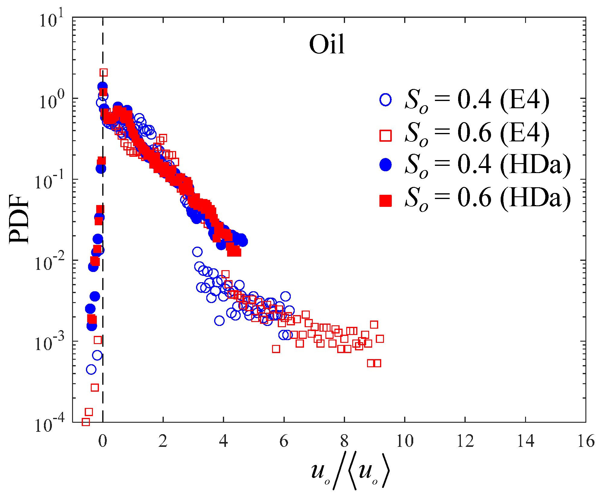
Figure A2.
Sample PDFs of , uw and , respectively being the horizontal component of the velocity vector of water phase and its mean. Full and empty symbols respectively are associated with sample HDa and E4. Blue circles and red squares respectively correspond to So = 0.4, 0.6. The dashed line identifies the peak value of the sample PDFs.
References
- Dullien, F.A.L. Porous Media Fluid Transport and Pore Structure, 2nd ed.; Academic: San Diego, CA, USA, 1992. [Google Scholar]
- Sahimi, M. Flow and Transport in Porous Media and Fractured Rock; Wiley VCH: Weinheim, Germany, 1995. [Google Scholar]
- Auriault, J.L.; Adler, P.M. Taylor dispersion in porous media: Analysis by multiple scale expansions. Adv. Water Resour. 1995, 4, 217–226. [Google Scholar] [CrossRef]
- Auriault, J.L. Non saturated deformable porous media: Quasistatic. Transp. Porous Media 1987, 2, 45–64. [Google Scholar] [CrossRef]
- Wood, B.D.; Valdès-Parada, F.J. Volume averaging: Local and nonlocal closures using a Green’s function approach. Adv. Water Resour. 2013, 51, 139–167. [Google Scholar] [CrossRef]
- Luévano-Rivas, O.A.; Valdés-Parada, F.J. Upscaling immiscible two-phase dispersed flow in homogeneous porous media: A mechanical equilibrium approach. Chem. Eng. Sci. 2015, 126, 116–131. [Google Scholar] [CrossRef]
- Alvarez-Ramirez, J.; Valdes-Parada, F.J.; Ibarra-Valdez, C. An Ohm’s law analogy for the effective diffusivity of composite media. Physica A 2016, 447, 141–148. [Google Scholar] [CrossRef]
- Auriault, J.L. Dynamics of two immiscible fluids flowing through deformable porous media. Transp. Porous Media 1989, 4, 105–128. [Google Scholar] [CrossRef]
- Withaker, S. Flow in porous media II: The governing equations for immiscible, two phase flow. Transp. Porous Media 1986, 105–125. [Google Scholar] [CrossRef]
- Whitaker, S. The closure problem for two-phase flow in homogeneous porous media. Chem. Eng. Sci. 1994, 49, 5. [Google Scholar] [CrossRef]
- Porta, G.M.; Chaynikov, S.; Riva, M.; Guadagnini, A. Upscaling solute transport in porous media from the pore scale to dual- and multi-continuum formulations. Water Resour. Res. 2013, 49, 2025–2039. [Google Scholar] [CrossRef]
- Gray, W.; Miller, C. Introduction to the Thermodynamically Constrained Averaging Theory; Springer: New York, NY, USA, 2014. [Google Scholar]
- Avraam, D.G.; Payatakes, A.C. Flow regimes and relative permeabilities during steady-state two-phase flow in porous media. J. Fluid Mech. 1995, 293, 207–236. [Google Scholar] [CrossRef]
- Tallakstad, K.T.; Knudsen, H.A.; Ramstad, T.; Løvoll, G.; Måløy, K.J.; Toussaint, R.; Flekkøy, E.G. Steady-state two-phase flow in porous media: Statistics and transport properties. Phys. Rev. Lett. 2009, 102, 074502. [Google Scholar] [CrossRef] [PubMed]
- Li, H.; Pan, C.; Miller, C.T. Pore-scale investigation of viscous coupling effects for two-phase flow in porous media. Phys. Rev. E 2005, 72, 026705. [Google Scholar] [CrossRef] [PubMed]
- Huang, H.; Lu, X. Relative permeabilities and coupling effects in steady-state gas-liquid flow in porous media: A lattice Boltzmann study. Phys. Fluids 2009, 21, 092104. [Google Scholar] [CrossRef]
- Ahmadlouydarab, M.; Liu, Z.S.; Feng, J.J. Relative permeability for two-phase flow through corrugated tubes as model porous media. Int. J. Multiphas. Flow 2012, 47, 85–93. [Google Scholar] [CrossRef]
- Andrew, M.; Bijeljic, B.; Blunt, M.J. Pore-scale contact angle measurements at reservoir conditions using X-ray microtomography. Adv. Water Resour. 2014, 68, 24–31. [Google Scholar] [CrossRef]
- Scanziani, A.; Singh, K.; Blunt, M.J.; Guadagnini, A. Automatic method for estimation of in situ contact angle from X-ray micro tomography images of two-phase flow in porous media. J. Colloid Interface Sci 2017, in press. [Google Scholar] [CrossRef] [PubMed]
- Trojer, M.; Szulczewski, M.L.; Juanes, R. Stabilizing fluid-fluid displacements in porous media through wettability alteration. Phys. Rev. Appl. 2015, 3, 054008. [Google Scholar] [CrossRef]
- Dou, Z.; Zhou, Z.F. Numerical study of non-uniqueness of the factors influencing relative permeability in heterogeneous porous media by lattice Boltzmann method. Int. J. Heat Fluid Flow 2013, 42, 23–32. [Google Scholar] [CrossRef]
- Liu, H.; Valocchi, A.J.; Werth, C.; Kang, Q.; Oostrom, M. Pore-scale simulation of liquid CO2 displacement of water using a two-phase lattice Boltzmann model. Adv. Water. Resour. 2014, 73, 144–158. [Google Scholar] [CrossRef]
- Jiang, Z.; van Dijke, M.I.J.; Wu, K.; Couples, G.D.; Sorbie, K.S.; Ma, J. Stochastic pore network generation from 3D rock images. Transp. Porous Med. 2012, 94, 571–593. [Google Scholar] [CrossRef]
- Ahmadi, A.; Aigueperse, A.; Quintard, M. Calculation of the effective properties describing active dispersion in porous media: From simple to complex unit cells. Adv. Water Resour. 2001, 24, 423–438. [Google Scholar] [CrossRef]
- Bahar, T.; Golfier, F.; Oltéan, C.; Benioug, M. An upscaled model for bio-enhanced NAPL dissolution in porous media. Transp. Porous Med. 2016, 113, 653–693. [Google Scholar] [CrossRef]
- Lugo-Méndez, H.D.; Valdés-Parada, F.J.; Porter, M.L.; Wood, B.D.; Ochoa-Tapia, J.A. Upscaling diffusion and nonlinear reactive mass transport in homogeneous porous media. Transp. Porous Med. 2015, 107, 683–716. [Google Scholar] [CrossRef]
- Icardi, M.; Boccardo, G.; Tempone, R. On the predictivity of pore-scale simulations: Estimating uncertainties with multilevel Monte Carlo. Adv. Water Resour. 2016, 95, 46–60. [Google Scholar] [CrossRef]
- Hyman, J.D.; Smolarkiewicz, P.K.; Winter, C.L. Heterogeneities of flow in stochastically generated porous media. Phys. Rev. E 2012, 86, 056701. [Google Scholar] [CrossRef] [PubMed]
- Siena, M.; Riva, M.; Hyman, J.D.; Winter, C.L.; Guadagnini, A. Relationship between pore size and velocity probability distributions in stochastically generated porous media. Phys. Rev. E 2014, 89, 013018. [Google Scholar] [CrossRef] [PubMed]
- Hyman, J.D.; Winter, C.L. Stochastic generation of explicit pore structures by thresholding Gaussian random fields. J. Comput. Phys. 2014, 277, 16–31. [Google Scholar] [CrossRef]
- Hyman, J.D.; Smolarkiewicz, P.K.; Winter, C.L. Pedotransfer functions for permeability: A computational study at pore scales. Water Resour. Res. 2013, 49, 2080–2092. [Google Scholar] [CrossRef]
- Hyman, J.D.; Winter, C.L. Hyperbolic regions in flows through three-dimensional pore structures. Phys. Rev. E 2013, 88, 063014. [Google Scholar] [CrossRef] [PubMed]
- Guadagnini, A.; Blunt, M.; Riva, M.; Bijeljic, B. Statistical scaling of geometric characteristics in millimeter scale natural porous media. Trans. Porous Med. 2014, 101, 465–475. [Google Scholar] [CrossRef]
- Hyman, J.D.; Guadagnini, A.; Winter, C.L. Statistical scaling of geometric characteristics in stochastically generated pore microstructures. Computat. Geosci. 2015, 19, 845–854. [Google Scholar] [CrossRef]
- Dong, H.; Blunt, M.J. Pore-network extraction from micro-computerized-tomography images. Phys. Rev. E 2009, 80, 036307. [Google Scholar] [CrossRef] [PubMed]
- Mantz, H.; Jacobs, K.; Mecke, K. Utilizing Minkowski functionals for image analysis: A marching square algorithm. J. Stat. Mech. 2008, 2008, P12015. [Google Scholar] [CrossRef]
- Vogel, H.J.; Roth, K. Quantitative morphology and network representation of soil pore structure. Adv. Water Resour. 2001, 24, 233–242. [Google Scholar] [CrossRef]
- Vogel, H.J.; Weller, U.; Schlüter, S. Quantification of soil structure based on Minkowski functions. Comput. Geosci. 2010, 36, 1236–1245. [Google Scholar] [CrossRef]
- Schlüter, S.; Vogel, H.J. On the reconstruction of structural and functional properties in random heterogeneous media. Adv. Water Resour. 2011, 34, 314–325. [Google Scholar] [CrossRef]
- COMSOL Multiphysics®. CFD Module User’s Guide, Version 4.4; Comsol Inc.: Burlington, MA, USA, 2013. [Google Scholar]
- Badalassi, V.E.; Ceniceros, H.D.; Banerjee, S. Computation of multiphase systems with phase field models. J. Comput. Phys. 2003, 190, 317–397. [Google Scholar] [CrossRef]
- Yue, P.; Feng, J.J.; Liu, C.; Shen, J. A diffuse-interface method for simulating two-phase flows of complex fluids. J. Fluid Mech. 2004, 515, 293–317. [Google Scholar] [CrossRef]
- Amiri, H.A.A.; Hamouda, A.A. Evaluation of level set and phase field methods in modeling two phase flow with viscosity contrast through dual-permeability porous medium. Int. J. Multiphas. Flow 2013, 52, 22–34. [Google Scholar] [CrossRef]
- Amiri, H.A.A.; Hamouda, A.A. Pore-scale modeling of non-isothermal two phase flow in 2D porous media: Influences of viscosity, capillarity, wettability and heterogeneity. Int. J. Multiphas. Flow 2014, 61, 14–27. [Google Scholar] [CrossRef]
- Yue, P.; Zhou, C.; Feng, J.J.; Ollivier-Gooch, C.F.; Hu, H.H. Phase-field simulations of interfacial dynamics in viscoelastic fluids using finite elements with adaptive meshing. J. Comput. Phys. 2006, 219, 47–67. [Google Scholar] [CrossRef]
- Yue, P.; Zhou, C.; Feng, J.J. Spontaneous shrinkage of drops and mass conservation in phase-field simulations. J. Comput. Phys. 2007, 223, 1–9. [Google Scholar] [CrossRef]
- Beal, C. The viscosity of air, water, natural gas, crude oil and its associated gases at oil field temperature and pressure. Trans. AIME 1946, 165, 94–115. [Google Scholar] [CrossRef]
- Whitaker, S. The Method of Volume Averaging; Kluwer Academic Publishers: Dordrecht, The Netherlands, 1999. [Google Scholar]
- Auriault, J.L.; Boutin, C.; Geindreau, C. Homogenization of Coupled Phenomena in Heterogeneous Media; Iste Wiley: London, UK, 2009. [Google Scholar]
- Chang, L.C.; Chen, H.H.; Shan, H.Y.; Tsai, J.P. Effect of connectivity and wettability on the relative permeability of NAPLs. Environ. Geol. 2009, 56, 1437–1447. [Google Scholar] [CrossRef]
Figure 1.
Regular elementary cells (a) HDa, (b) HDb, (c) HDc and randomly generated elementary cells (d) E1, (e) E2, (f) E3, (g) E4, (h) E5, (i) E6, (j) E7, (k) E8, and (l) E9. Gray and white regions respectively correspond to the solid matrix and to the pore space. Horizontal dashed-dotted lines indicate axes of symmetry of the systems. Lx: size of the medium along x-; Ly: size of the medium along y-; Dg: grain diameter; Dt: throat diameter.
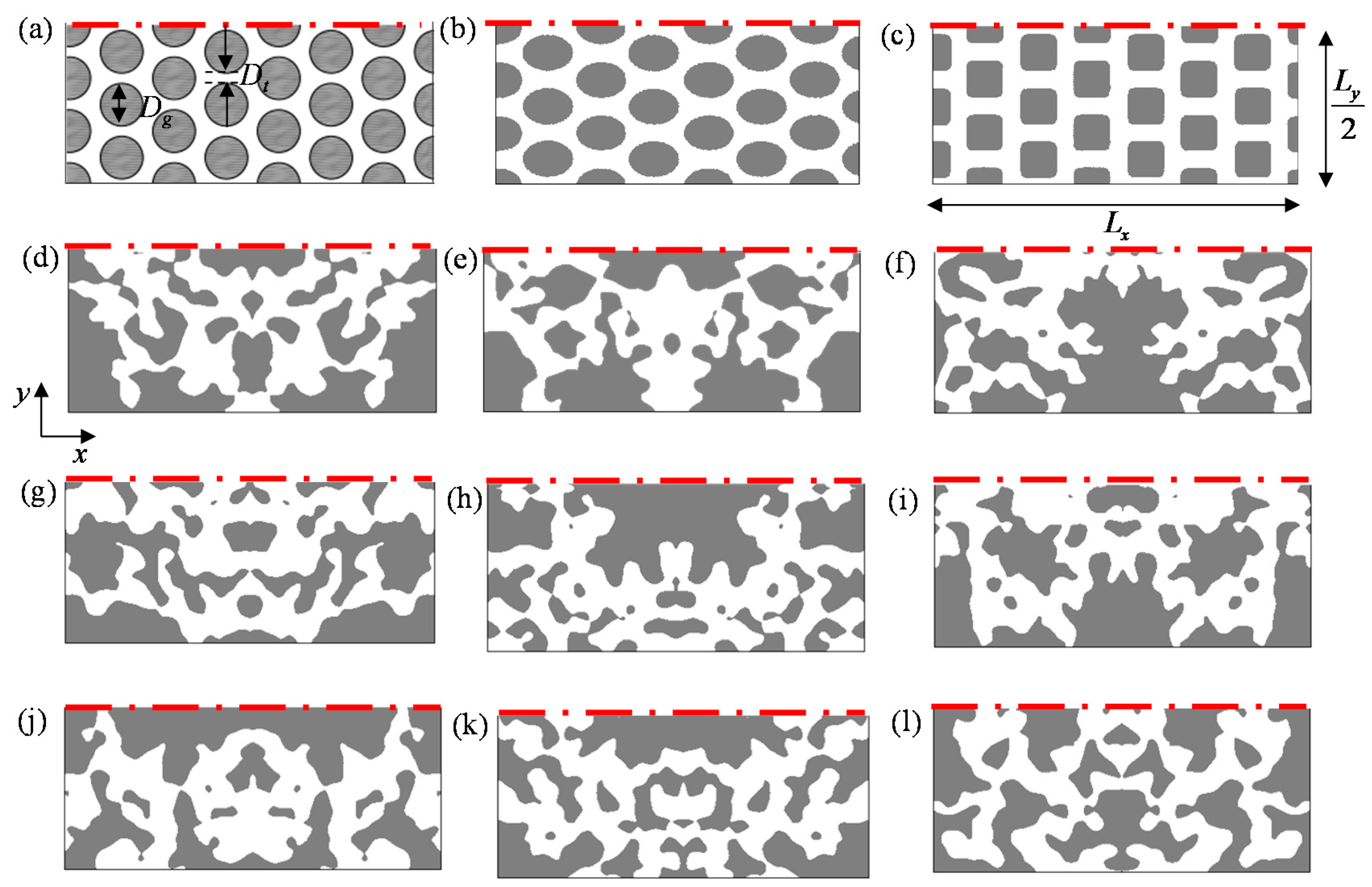
Figure 2.
Relative frequency of the coordination number in the random samples Ei (i = 1, ..., 9).
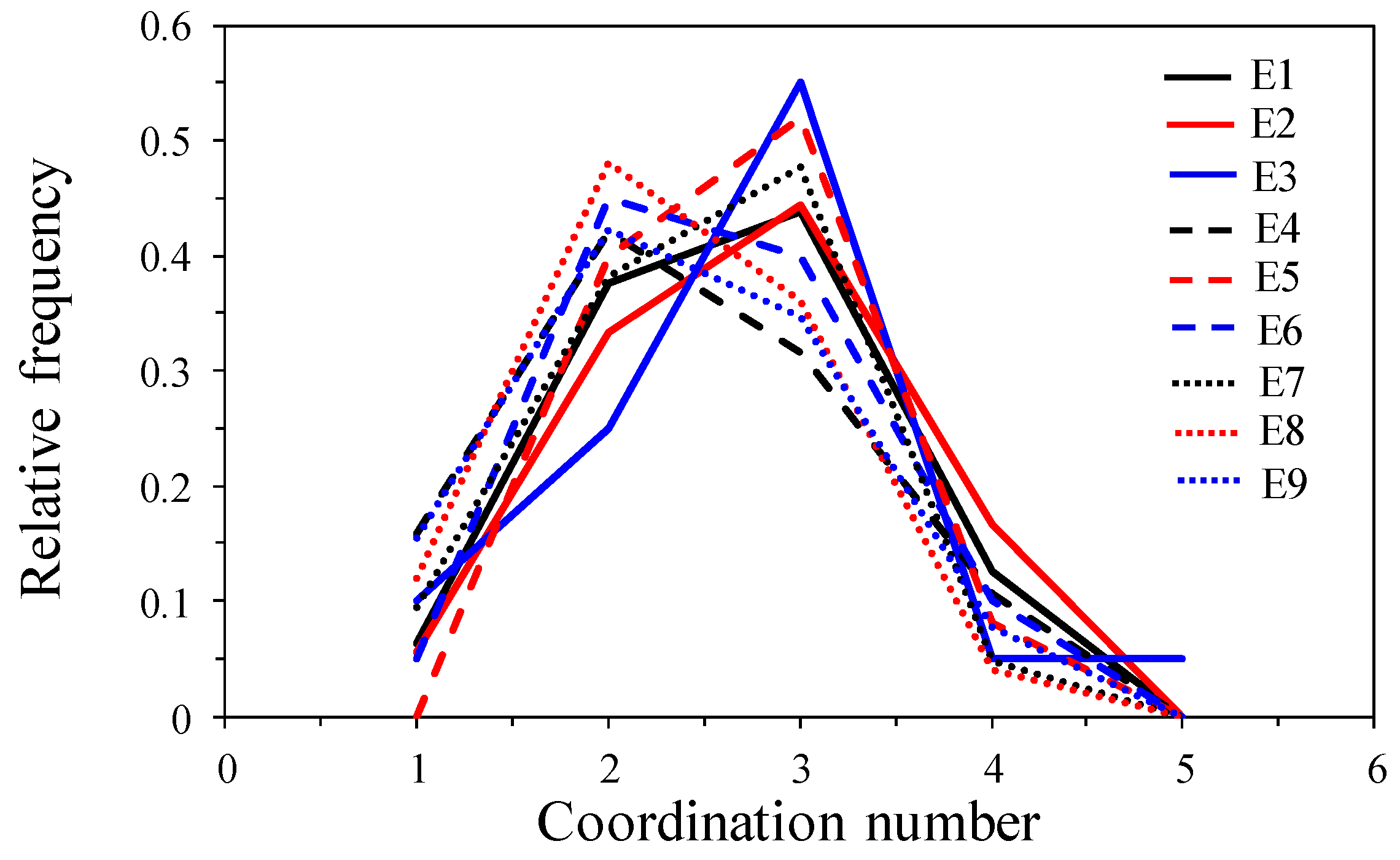
Figure 3.
Histogram of tortuosity, , and particle trajectories through the elementary cells (color scale expressed in terms of local normalized velocity , being the norm of the velocity vector v and its mean) for (a) HDa, (b) E1, (c) E4, and (d) E8. Vertical dashed lines correspond to mean tortuosity. Horizontal dashed-dotted lines indicate the axes of symmetry of the systems.

Figure 4.
Example of initial oil (red) and water (blue) phase distribution pattern within (a) HDa and (b) E4 for So = 0.5. Horizontal dashed-dotted lines indicate axes of symmetry of the systems.
Figure 4.
Example of initial oil (red) and water (blue) phase distribution pattern within (a) HDa and (b) E4 for So = 0.5. Horizontal dashed-dotted lines indicate axes of symmetry of the systems.

Figure 5.
Distribution of the two phases (oil, in red; water, in blue) at steady state with θ = 90° for (a) HDa and So = 0.42, (b) E1 and So = 0.49, (c) E4 and So = 0.50, and (d) E8 and So = 0.49. Streamlines of the flow field are plotted as white curves.
Figure 5.
Distribution of the two phases (oil, in red; water, in blue) at steady state with θ = 90° for (a) HDa and So = 0.42, (b) E1 and So = 0.49, (c) E4 and So = 0.50, and (d) E8 and So = 0.49. Streamlines of the flow field are plotted as white curves.
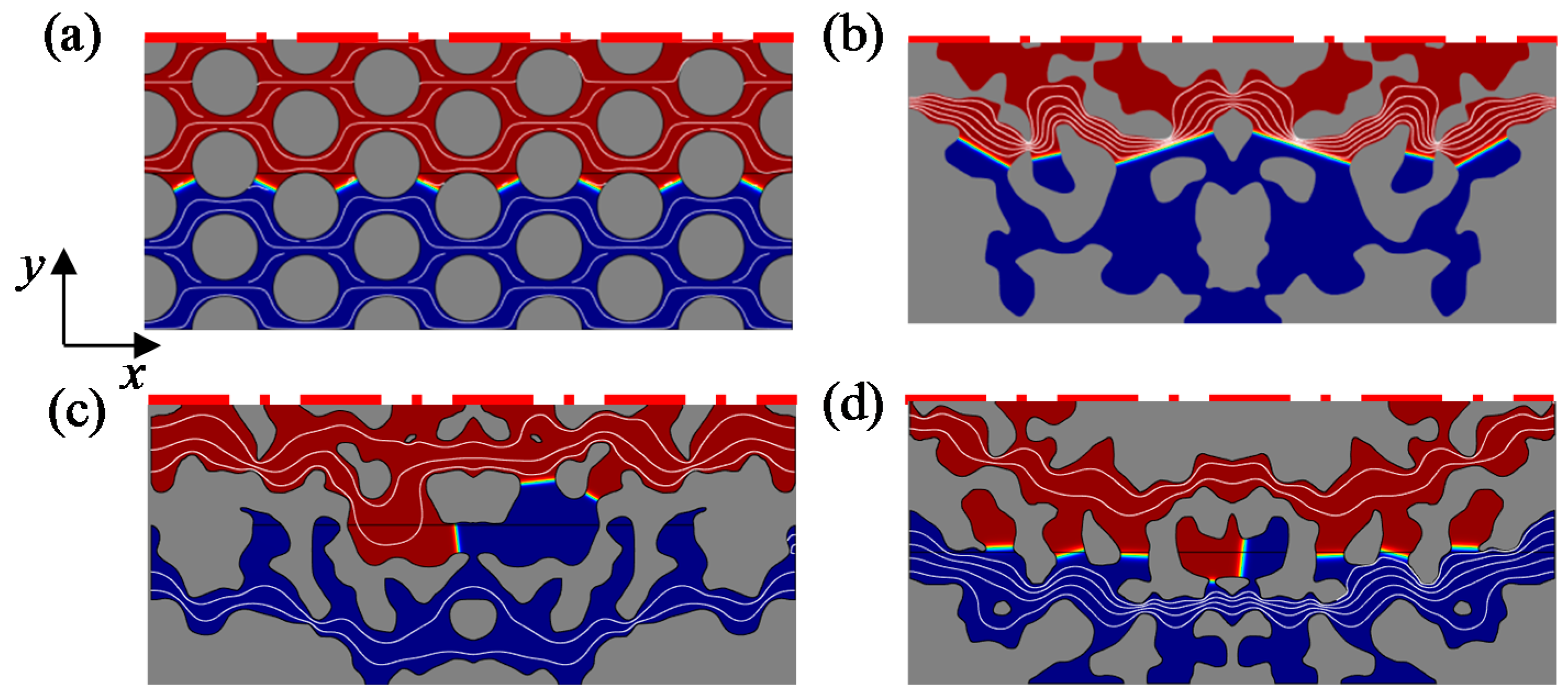
Figure 6.
Spatial distribution of the two phases (oil, in red; water, in blue) at steady state with θ = 60° (WW) and θ = 120° (OW) at (a) HDa with So = 0.53 (WW) and So = 0.47 (OW); (b) E1 with So = 0.53 (WW) and So = 0.56 (OW); (c) E4 with So = 0.48 (WW) and So = 0.52 (OW); and (d) E8 with So = 0.49 (WW) and So = 0.47 (OW). Streamlines of the flow field are plotted as white curves. WW: water wet, OW: oil wet.
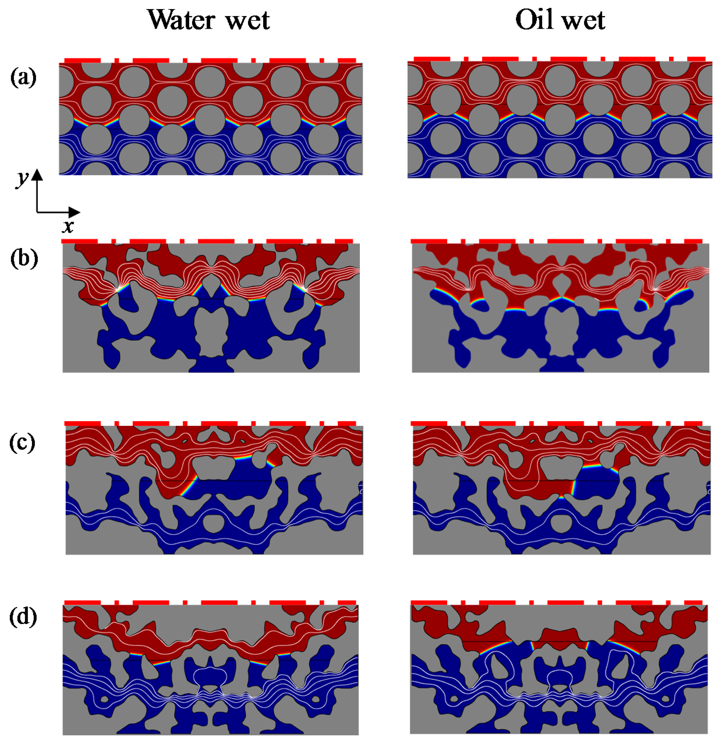
Figure 7.
Relative permeability curves () in (a) HDa, (b) HDb, (c) HDc, (d) E1, (e) E4, and (f) E8 for: θ = 90° (NW), θ = 60° (WW) and θ = 120° (OW). NW: neutral wet.
Figure 7.
Relative permeability curves () in (a) HDa, (b) HDb, (c) HDc, (d) E1, (e) E4, and (f) E8 for: θ = 90° (NW), θ = 60° (WW) and θ = 120° (OW). NW: neutral wet.
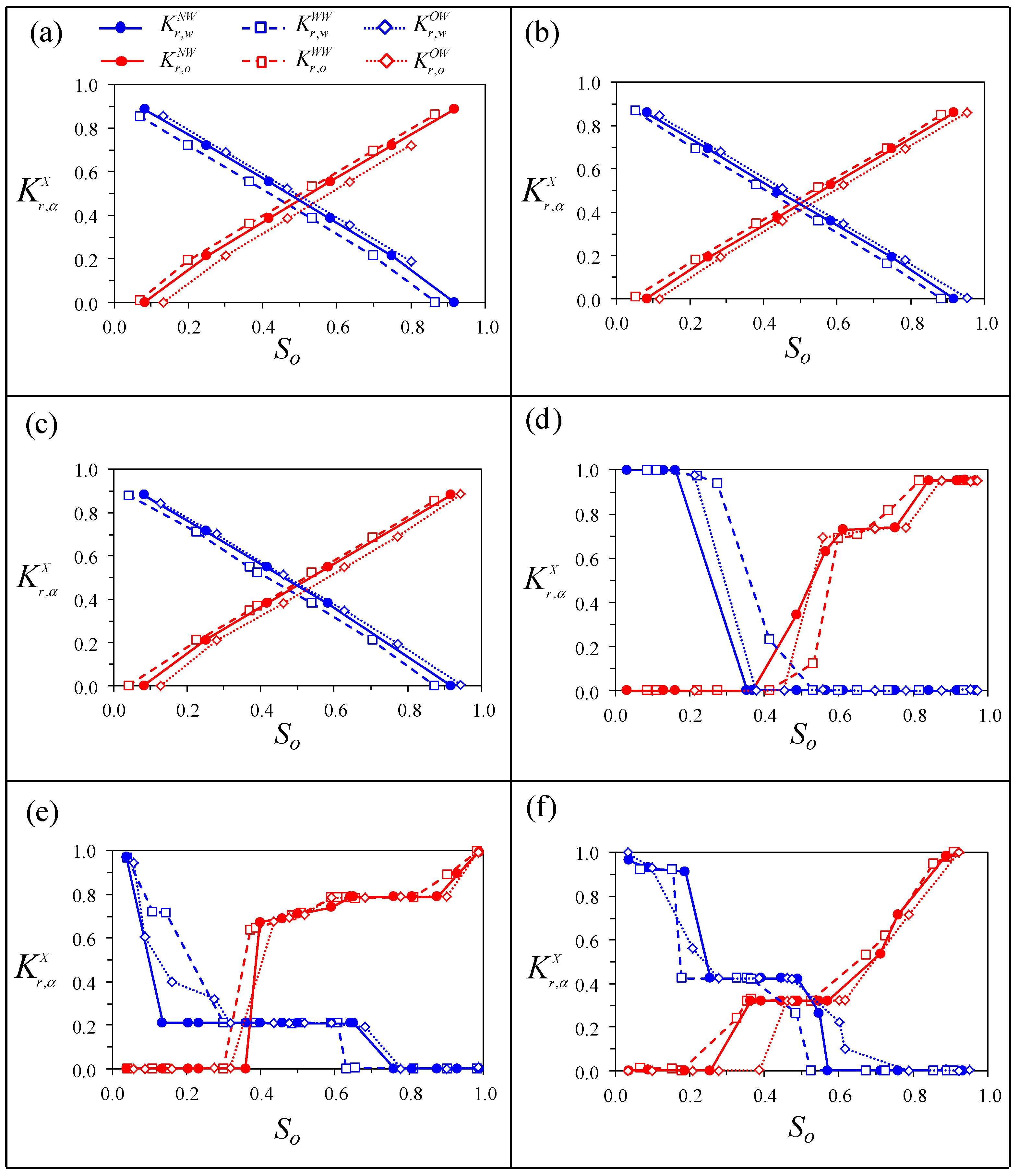
Figure 8.
Relative permeability curves in the three regular settings (thick curves) and in the nine heterogeneous elementary cells (thin curves) for (a) θ = 90° (NW), (b) θ = 60° (WW), (c) θ = 120° (OW).
Figure 8.
Relative permeability curves in the three regular settings (thick curves) and in the nine heterogeneous elementary cells (thin curves) for (a) θ = 90° (NW), (b) θ = 60° (WW), (c) θ = 120° (OW).

Figure 9.
Comparison between relative permeability curves associated with our computational analyses (curves) and data from experimental studies on micromodels (symbols) of (a) Avraam and Payatakes [13]; and (b) Chang et al. [50]. Red and black symbols in (b) are respectively associated with a Water/Diesel fuel system and Water / Tetrachloroethane tests. Open and solid circles respectively correspond to imbibition and drainage experiments (corresponding relative permeabilities are respectively indicated with superscripts I and D).

Table 1.
Connected porosity (n), Specific Surface Area (SSA), intrinsic permeability (K) and maximum likelihood (ML) estimates of range and sill ( and ; i = x, y) of directional variograms of the indicator function of the pore space.
Table 1.
Connected porosity (n), Specific Surface Area (SSA), intrinsic permeability (K) and maximum likelihood (ML) estimates of range and sill ( and ; i = x, y) of directional variograms of the indicator function of the pore space.
| Sample Identifier | n | SSA (10−3 m−1) | K (10−10 m2) | ||||
|---|---|---|---|---|---|---|---|
| HDa | 0.48 | 8.63 | 4.97 | - | - | - | - |
| HDb | 0.50 | 8.63 | 11.67 | - | - | - | - |
| HDc | 0.52 | 8.63 | 10.47 | - | - | - | - |
| Average HDa–HDc | 0.50 | 8.63 | 9.06 | - | - | - | - |
| E1 | 0.48 | 8.39 | 1.25 | 0.12 | 0.23 | 0.12 | 0.21 |
| E2 | 0.49 | 7.84 | 2.42 | 0.16 | 0.25 | 0.17 | 0.23 |
| E3 | 0.48 | 8.61 | 3.43 | 0.17 | 0.25 | 0.12 | 0.22 |
| E4 | 0.51 | 9.11 | 3.84 | 0.11 | 0.21 | 0.13 | 0.23 |
| E5 | 0.49 | 9.24 | 4.43 | 0.18 | 0.26 | 0.14 | 0.24 |
| E6 | 0.50 | 8.20 | 2.29 | 0.16 | 0.25 | 0.21 | 0.24 |
| E7 | 0.49 | 7.69 | 1.01 | 0.12 | 0.22 | 0.25 | 0.27 |
| E8 | 0.49 | 9.44 | 3.11 | 0.13 | 0.24 | 0.16 | 0.27 |
| E9 | 0.49 | 9.13 | 1.04 | 0.14 | 0.27 | 0.13 | 0.24 |
| Average E1–E9 | 0.49 | 8.63 | 2.54 | 0.14 | 0.24 | 0.16 | 0.24 |
Table 2.
Topological and morphological information of the elementary cells: total number of pores, Npores; average coordination number, ; ratio ; area of the solid phase, M0; boundary length between solid and fluid, M1; and Euler number, M2.
Table 2.
Topological and morphological information of the elementary cells: total number of pores, Npores; average coordination number, ; ratio ; area of the solid phase, M0; boundary length between solid and fluid, M1; and Euler number, M2.
| Sample Identifier | Npores | (%) | M0 (10−6 m2) | M1 (10−3 m) | M2 | |
|---|---|---|---|---|---|---|
| HDa | 112 | 3.00 | 2.68 | 8.10 | 69.91 | −173.25 |
| HDb | 112 | 3.00 | 2.68 | 8.53 | 73.19 | −181.00 |
| HDc | 112 | 3.00 | 2.68 | 10.73 | 80.77 | −64.25 |
| Average HDa–HDc | 112 | 3.00 | 2.68 | 9.12 | 74.62 | −139.50 |
| E1 | 64 | 2.63 | 4.10 | 7.20 | 60.45 | −145.25 |
| E2 | 72 | 2.72 | 3.78 | 7.03 | 55.10 | −133.25 |
| E3 | 80 | 2.70 | 3.38 | 7.16 | 61.61 | −147.50 |
| E4 | 76 | 2.37 | 3.12 | 6.74 | 61.39 | −160.75 |
| E5 | 100 | 2.68 | 2.68 | 6.95 | 64.24 | −151.00 |
| E6 | 80 | 2.55 | 3.19 | 6.87 | 56.28 | −134.25 |
| E7 | 84 | 2.48 | 2.95 | 7.06 | 54.30 | −135.75 |
| E8 | 100 | 2.32 | 2.32 | 9.44 | 65.62 | −162.50 |
| E9 | 104 | 2.35 | 2.26 | 9.13 | 63.93 | −157.75 |
| Average E1–E9 | 84.4 | 2.53 | 3.09 | 6.99 | 60.32 | −147.56 |
Table 3.
Number of percolating particles, NP, and basic statistics of tortuosity, .
| Sample Identifier | Np | Mean | Variance | Minimum | Maximum | Skewness | Kurtosis |
|---|---|---|---|---|---|---|---|
| HDa | 4906 | 1.18 | 1.5 × 10⁻⁴ | 1.06 | 1.21 | 0.44 | 1.00 |
| HDb | 4947 | 1.14 | 6.5 × 10⁻⁵ | 0.96 | 1.16 | −9.33 | 197.76 |
| HDc | 4935 | 1.21 | 3.3 × 10⁻⁴ | 1.13 | 1.27 | 1.27 | 3.87 |
| Average HDa–HDc | 4929 | 1.18 | 1.8 × 10⁻⁴ | 1.05 | 1.21 | −2.54 | 67.54 |
| E1 | 4726 | 1.30 | 5.3 × 10⁻³ | 1.21 | 1.51 | 0.56 | 2.64 |
| E2 | 2305 | 1.32 | 2.0 × 10⁻² | 1.15 | 1.92 | 0.71 | 3.46 |
| E3 | 2422 | 1.34 | 5.4 × 10⁻² | 1.12 | 2.14 | 1.23 | 3.43 |
| E4 | 3729 | 1.17 | 3.7 × 10⁻³ | 1.09 | 1.42 | 0.63 | 2.81 |
| E5 | 3471 | 1.42 | 2.7 × 10⁻² | 1.18 | 1.74 | 0.54 | 1.97 |
| E6 | 3730 | 1.80 | 2.6 × 10⁻² | 1.15 | 2.11 | −1.32 | 7.85 |
| E7 | 3151 | 1.26 | 8.7 × 10⁻³ | 1.15 | 1.66 | 1.21 | 3.67 |
| E8 | 4480 | 1.21 | 1.2 × 10⁻² | 1.06 | 1.42 | 0.06 | 1.59 |
| E9 | 4697 | 1.17 | 3.7 × 10⁻³ | 1.09 | 1.42 | 0.64 | 2.76 |
| Average E1–E9 | 3635 | 1.33 | 8.1 × 10⁻³ | 1.10 | 1.50 | 0.64 | 2.67 |
Table 4.
Physicochemical properties of fluids employed by Avraam and Payatakes [13], and Chang et al. [50] and used in this study.
| Property | Experiments from Avraam and Payatakes [13] | Experiments from Chang et al. [50] | Our Computations | |
|---|---|---|---|---|
| Non wetting fluid | n-Dodecane | Diesel Fuel/Tetrachloroethane | Oil | |
| Wetting fluid | Water | Water | Water | |
| (Pa s) | 1.36 × 10⁻³ | not specified | 2.0 × 10⁻³ | |
| (Pa s) | 0.94 × 10⁻³ | not specified | 1.0 × 10⁻³ | |
| 1.45 | not specified | 2.0 | ||
| (kg/m3) | 730 | 820/1600 | 1000 | |
| (kg/m3) | 995 | 997 | 1000 | |
| (mN/m) | 25 | 48.7/38.75 | 40.0 | |
| (°) | 40 | 0 | 60 | |
| Capillary Number | 1.19 × 10⁻⁵ | not specified | 10−4 |
µα: dynamic viscosity of phase α (α = o or w for oil and water phase, respectively), ρα: density of phase α (α = o or w), σ: interfacial tension, θ: contact angle.
© 2017 by the authors. Licensee MDPI, Basel, Switzerland. This article is an open access article distributed under the terms and conditions of the Creative Commons Attribution (CC BY) license (http://creativecommons.org/licenses/by/4.0/).
Share and Cite
MDPI and ACS Style
Bianchi Janetti, E.; Riva, M.; Guadagnini, A. Effects of Pore-Scale Geometry and Wettability on Two-Phase Relative Permeabilities within Elementary Cells. Water 2017, 9, 252. https://doi.org/10.3390/w9040252
AMA Style
Bianchi Janetti E, Riva M, Guadagnini A. Effects of Pore-Scale Geometry and Wettability on Two-Phase Relative Permeabilities within Elementary Cells. Water. 2017; 9(4):252. https://doi.org/10.3390/w9040252
Chicago/Turabian StyleBianchi Janetti, Emanuela, Monica Riva, and Alberto Guadagnini. 2017. "Effects of Pore-Scale Geometry and Wettability on Two-Phase Relative Permeabilities within Elementary Cells" Water 9, no. 4: 252. https://doi.org/10.3390/w9040252
Note that from the first issue of 2016, this journal uses article numbers instead of page numbers. See further details here.