
Seasonal Variation in Sediment Oxygen Demand in a Northern Chained River-Lake System


Global Institute for Water Security, University of Saskatchewan, 11 Innovation Boulevard, Saskatoon, SK S7N 3H5, Canada
*
Author to whom correspondence should be addressed.
Water 2017, 9(4), 254; https://doi.org/10.3390/w9040254
Submission received: 21 January 2017
/
Revised: 30 March 2017
/
Accepted: 30 March 2017
/
Published: 5 April 2017
(This article belongs to the Special Issue River and Lake Ice Processes—Impacts of Freshwater Ice on Aquatic Ecosystems in a Changing Globe)
Abstract
:Sediment oxygen demand (SOD) contributes immensely to hypolimnetic oxygen depletion. SOD rates thus play a key role in aquatic ecosystems’ health predictions. These rates, however, can be very expensive to sample. Moreover, determination of SOD rates by sediment diagenesis modeling may require very large datasets, or may not be easily adapted to complex aquatic systems. Water quality modeling for northern aquatic systems is emerging and little is known about the seasonal trends of SOD rates for complex aquatic systems. In this study, the seasonal trend of SOD rates for a northern chained river-lake system has been assessed through the calibration of a water quality model. Model calibration and validation showed good agreement with field measurements. Results of the study show that, in the riverine section, SOD20 rates decreased from 1.9 to 0.79 g/m2/day as urban effluent traveled along the river while a SOD20 rate of 2.2 g/m2/day was observed in the lakes. Seasonally, the SOD20 rates in summer were three times higher than those in winter for both river and lakes. The results of the study provide insights to the seasonal trend of SOD rates especially for northern rivers and lakes and can, thus, be useful for more complex water quality modeling studies in the region.
1. Introduction
Oxygen depletion in aquatic ecosystems has received much attention in the world. The importance of sediments in oxygen depletion have been well studied by many authors [1,2]. Oxidation (aerobic decomposition) of settled organic materials and the anaerobic respiration of invertebrates in sediments have been found to consume a large percentage of water column oxygen in surface water bodies [3,4]. Oxygen is used during the decomposition of organic matter by microorganisms and as it reacts with the by-products of respiration. The stabilization of organic material by organisms (e.g., bacteria) can exert high oxygen demand in sediments. High benthic oxygen demand can also result from high primary production by benthic algae (periphyton). Oxygen is consumed when algae respires in the night and it is produced during photosynthesis in the day. Studies by authors [5,6] indicated that oxygen demand by sediments was the major source of water column oxygen depletion. Benthic deposits usually originate from surface runoff, wastewater effluents, and aquatic conditions [7,8,9]. Once at the receiving surface water, the deposits are transported from these allochthonous materials through the water column to the river bed. The deposits could also be generated from autochthonous materials as aquatic plants and phytoplankton die off [10,11]. Extremely low levels of oxygen (below 2–3 mg/L) in aquatic systems may lead to dead zones [12], and flaura and fauna death. The rate at which water column oxygen is removed during the decomposition of organic matter and respiration of organisms in stream or lake bed sediments is known as sediment oxygen demand (SOD) [13,14,15].
SOD is influenced by temperature, velocity of water flow, residence time, and sediment composition [16]. An increase in water temperature accelerates, for example, the rate at which benthic bacteria respire, which elevates the SOD rate. Investigations by [17] show that a 10 °C rise in temperature doubled biological activities in sediments. MacPherson et al. [7] also found that SOD rate positively correlates with temperature. At low velocity (<10 cm/s), the SOD rate has been found to increase, but it decreases at higher velocity [18]. Since SOD plays a key role in the dissolved oxygen balance of surface water bodies at the sediment-water interface, determining its value in water quality modeling is paramount to the overall prediction of the health of aquatic ecosystems.
SOD can be estimated by in situ and laboratory measurements, sediment diagenesis modeling or through water quality model calibration. Liu and Chen [19] conducted SOD measurements along the Xindian River of Northern Taiwan for the purpose of water quality modeling. The authors found that SOD rates were directly proportional to the river discharge—higher discharge resulted in lower SOD rates. SOD rates at 20 °C ranged from 0.367 to 1.246 g/m2/day. In the study by [15], the profile method was used to measure SOD rates in the Millstone River, Georgia. SOD ranged from 0.5 to 2.2 g/m2/day. Caldwell and Doyle [20] also conducted in situ SOD measurements along a river using SOD chambers. The measured SOD rates corrected to a temperature of 20 °C ranged from 1.3 to 4.1 g/m2/day. Several sediment diagenesis models have been built since 1996 to estimate the chemical concentrations and reaction rates often lacking from in-situ or laboratory measurements [21]. The study by [22] used a sediment diagenesis model to illustrate the influence of resuspension on the water column, and oxidation and denitrification in sediments. Sohma et al. [23,24,25] assessed the effect of water column anoxic fluctuations on sediment using a three-dimensional sediment diagenesis model. Calibrating the zero order SOD rate of a water quality model is another approach used to estimate SOD rate. Gualtieri [26] assessed SOD rates of a river by calibrating a water quality model within the minimum and maximum values of reported SOD rates. The author found the influence of SOD on dissolved oxygen to be substantial at effluent outfalls.
Estimating SOD by measurement techniques can become expensive due to the spatial and seasonal variation of SOD. In most surface water systems, SOD rate varies considerably, spatially, and seasonally, due to varying sediment composition. Spatially, the rate of deposition, physical, and chemical composition of sediment beds which affect oxygen consumption for rivers and lakes are substantially different. Steep sections of a river will have more boulder or cobble deposition and fine sediments (silt or clay) settle in low-velocity reaches, and for lakes, cobbles and pebbles settle at the inlet (as the current of a river slows down due to resistance from the rather still body of water in the lake); beyond the inlet and up to obstructing structures, sand, silt, and clay are, respectively, deposited as the current becomes very slow. These different sediment beds result in different SOD rates [27]. Seasonal variation of temperature impacts the composition of benthic and microbial communities, which influences the rate of SOD. Biological and chemical reactions in sediments are also elevated with temperature rise. As a result of these variations, often a large number of measurements are required to fully characterize SOD dynamics. In addition to the different SOD configurations and seasonal variation of temperature, it is often challenging to relate measurements to external loads. Sediment diagenesis models have been developed to handle the biogeochemical reactions that occur at the water column-sediment interface. The models are, however, complex and not easily adaptable to solve site-specific issues, such as complex river systems with varying sediment configurations. In addition, a large amount of data is needed to accurately drive these models, which might not be easily available [28,29]. Except in the case of special studies, SOD data for modeling purposes are not routinely collected [30].
In this paper, the seasonal variation of SOD for a prairie chained river-lake system is examined using the Water Quality Analysis Simulation Program (WASP 7.52) (Athens, GA, USA). Under-ice surface water quality modeling is emerging in the northern climate regions, but not much is known about the seasonal trends of SOD, especially for a complex system like chained river-lakes. One objective of the study is to examine the seasonal trend of SOD through an accurate but inexpensive modeling approach. Another objective is to determine the variation of SOD between the river and lake parts of the system. The estimated SOD values from this study will be used to set up an advanced eutrophication model in the future.
For a complex aquatic ecosystem, constraining processes and calibrating the water quality and transport modules of a low complexity water quality model provide a reasonable SOD estimate for water quality models [31]. At a low water quality model complexity, like the Streeter and Phelps dissolved oxygen balance, other process parameters are constrained, allowing models to be properly calibrated to few parameters. Building a model by gradually adding complexity is a strategy adopted by some modelers [32]. Complex models increase the number of processes being modeled, the output variables, and parameters [32]. Apart from the uncertainties associated with the model structure (as not all physical processes might be adequately represented, or even included) and forcings in a complex model, calibrating to optimum parameters, is often difficult in the face of sparse input data, as is common at most sites. According to [33], building complex models should be accompanied by a corresponding incorporation of relevant model observations. This paper adopts a slightly modified form of the Streeter and Phelps dissolved oxygen balance model, to estimate the SOD rates. All other water quality processes including reaeration are constrained.
2. Materials and Methods
2.1. Overview of Study Area
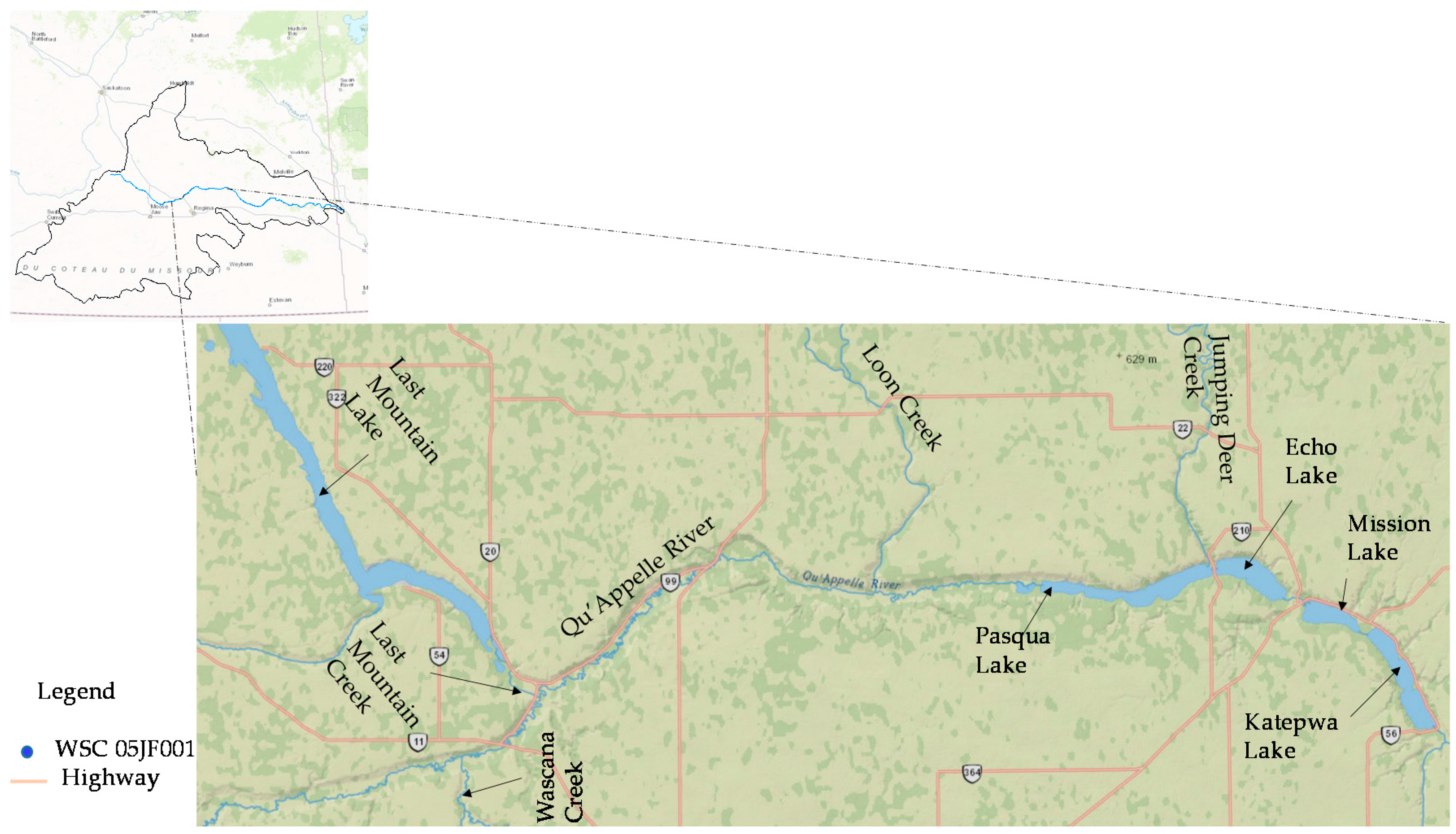
The study area is the Qu’Appelle River (QR) watershed, which extends eastward from Lake Diefenbaker in Saskatchewan to the Assiniboine River in Manitoba, Canada. Mainstay economic activities within the basin are agriculture (over 75% of total catchment area), fertilizer industries, underground and solution potash mines, oil refineries, and commercial fisheries. This study focused on the central lower half of the QR from the confluence of QR and Wascana Creek to Katepwa Lake (Figure 1). This section of the QR is a chained river-lake system, including four hypereutrophic lakes [34]: Pasqua, Echo, Mission, and Katepwa and an off-channel lake, Last Mountain Lake. A concrete control structure with timber stop-logs and lift gate on Echo Lake are used to regulate the water levels at Pasqua and Echo Lakes for recreational purposes. Water levels at Mission and Katepwa Lakes are maintained for commercial fishing by the regulation of a control structure at Katepwa Lake. The in-stream lakes have an average residence time of approximately nine days. Within the watershed two cities, Moose Jaw and Regina, release treated wastewater effluent into the river upstream of the lakes [34,35]. Tributaries from west to east include Wascana Creek, Last Mountain Creek, Loon Creek, Jumping Deer Creek, and Echo Creek. During floods, backflow from the Qu’Appelle is diverted through Last Mountain Creek into Last Mountain Lake. Echo Lake, Katepwa Lake, and Last Mountain Creek at Craven are equipped with control structures to regulate lake levels and to maintain environmental flow within the QR system.
The temperature in the region ranges from a mean of −16 °C in the winter to a mean of 19 °C in the summer. Mean annual potential evapotranspiration (600 mm) is twice the precipitation [35].
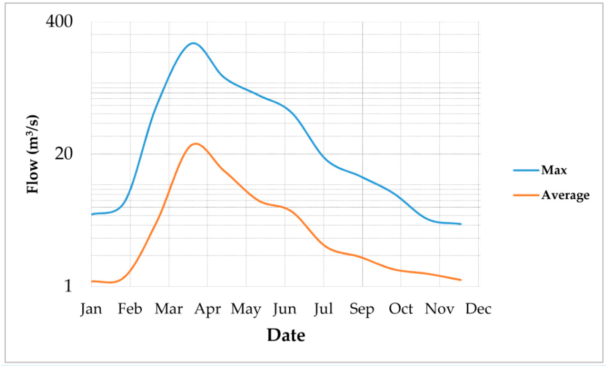
The Qu’Appelle River discharge is modified by interbasin transfer from the South Saskatchewan River. The flow regime depicts the characteristics of a typical prairie river and lake drainage setting (Figure 2). At the Water Survey of Canada (WSC) hydrometric station 05JF001, Lumsden, the monthly mean discharge below 4.29 m3/s occurs during the winter (November to March). During the spring, (March to April), monthly mean discharge increases sharply to 24.28 m3/s as a result of snowmelt. Discharge then decreases sharply until August and then levels off for the rest of the season.
During the winter season (November to March), the QR system is typically covered with ice and snow. Construction of the Qu’Appelle Dam was completed in 1967. Ice freeze-up and break-up conditions after the dam construction for the period 1970 to 2010 at WSC station 05JG006 is shown in Figure 3. The graph shows a steady increase to a late freeze-up and early break-up conditions.
2.2. Model Setup
The seasonal variation of sediment oxygen demand for the chained river-lake system of Qu’Appelle River valley was assessed using the Water Quality Analysis Simulation Program 7.52 (WASP) (Athens, GA, USA). The WASP program dynamically models the water column and underlying benthos of aquatic systems including rivers, lakes, estuaries and coastal water bodies. The program is used to simulate conventional and toxic water pollution problems based on the principles of conservation of mass, momentum, and energy. Model development includes discretizing the surface water network into one, two or three-dimensional segments and defining model boundary conditions and input parameters. A one-dimensional model was considered for the river and shallow lake system. The system was assumed to be well-mixed laterally and vertically. The transport and kinetics of biochemical oxygen demand and dissolved oxygen (BOD-DO) dynamics of the study area were characterized in WASP’s eutrophication module (EUTRO). EUTRO can simulate the dynamics of up to four systems including dissolved oxygen balance, the nitrogen cycle, phosphorus cycle, and phytoplankton kinetics.
The BOD-DO dynamics selected in EUTRO represents the basic complexity (complexity 1) of processes and kinetics involved in the dissolved oxygen balance. The main processes (see Equations (1)–(3) below) involved in the WASP’s complexity 1 are atmospheric reaeration as a source of dissolved oxygen (DO) and as sinks, the total oxidation, and settling of oxidizable organic material and SOD. This low level of complexity (a slightly modified form of Streeter-Phelps) was selected to allow reasonable estimation of SOD through model calibration, by driving the model with a verified streamflow transport and constraining all other processes [31]. The total biochemical oxygen demand (TBOD), which represents oxidation of organic matter, is the main kinetic reaction for oxygen demanding materials in the water column. The particulate fraction of biologically oxidizable organic material gets settled out and is deposited in the sediments under low flow conditions. The deposition sometimes influences benthic sediment oxygen demand. In EUTRO, SOD is described for water column segments and seasonal changes are determined by the temperature coefficient [31].
where;
| d(TBOD)/dt | = | Rate of change of the concentration of oxygen required to mineralize organic matter in mg/L/day. This is corrected before comparison with field BOD5 data |
| = | Oxygen demand due to the oxidization of newly produced organic matter per day, mg/L/day | |
| = | Deoxygenation rate at 20 °C, 1/day | |
| T | = | Water temperature, °C |
| θd | = | Temperature coefficient |
| d(DO)/dt | = | Rate of change of dissolved oxygen concentration, mg/L/day |
| θ2 | = | Temperature coefficient |
| DO | = | Dissolved oxygen concentration, mg/L |
| = | Total Biochemical oxygen demand in mg/L | |
| vs3 | = | Organic matter settling velocity, m/day |
| D | = | Average segment depth, m |
| f D5 | = | Fraction dissolved TBOD |
| = | Reaeration rate at 20 °C, 1/day | |
| DOs | = | DO solubility at temperature T, mg/L |
| SODT | = | Sediment oxygen demand rate at T, g/m2/day |
| θ | = | Temperature coefficient |
2.3. Advective Transport
The river network within the study area was modeled using WASP’s dynamic stream transport module. Dynamic flow in the model is calculated using kinematic wave flow routing, ponded weir overflow, or backwater flow equations. The module requires river segments and flow information. Segment characteristics including lengths, widths, and depths for average flow conditions, as well as bottom slopes and Manning friction coefficients, are used to define the hydraulics of the system. Flow pathways and inflow time functions for the main channel and tributaries are used to define the river network and boundary conditions. Within the river, flow is established by upstream or tributary inflow boundary conditions. As the flow moves downstream, bottom slope and channel roughness control discharge variation.
The riverine section of the network was modeled as free flowing using the kinematic wave flow routine of the dynamic stream transport module. In WASP (Athens, GA, USA), this routine calculates flow wave propagation, which results in varying depths, volumes, flows, and velocities for the network. Flow is estimated by solving the one-dimensional continuity and momentum equations. River segments between the confluence with Loon Creek and the Qu’Appelle lakes were characterized as backwater flow while the four lakes were represented as ponded segments with weir overflow. WASP 7.52 (Athens, GA, USA) allows up to 25 segments for ponds. River segments upstream of the Loon Creek confluence were characterized as one-dimensional kinematic wave flow.
A calibrated and validated HEC-RAS model (Davis, CA, USA) was used to generate hydraulic parameters used as inputs for the dynamic flow routines in WASP (Athens, GA, USA). HEC-RAS (Davis, CA, USA) performs up to two-dimensional steady and unsteady flow hydraulic calculations for full network of natural and constructed channels [36]. HEC-RAS (Davis, CA, USA) river and lake cross-sections were generated from a 2013 digital elevation model (DEM), river depth survey and lake bathymetry survey of the site. The river network was discretized using an interval of 700 m in the riverine section and up to 2800 m in the lakes. This resulted in 175 one-dimensional horizontal water columns in WASP (Athens, GA, USA). Hydrodynamic parameters generated in HEC-RAS (Davis, CA, USA) included the depth exponent and multipliers, segment widths, and average depths. For the free-flow segments, the depth multiplier was taken as the cross-sectional average segment depth under average flow condition. In WASP (Athens, GA, USA), depth exponent controls channel shape. A depth exponent value of 0.3, representing an irregular cross-section was selected for these segments. Together with segment widths, slopes, and roughness factors, these depths are used to estimate segment depths during simulations. In the same vein, depth multipliers for backwater flow segments and ponded segments were taken as the cross-sectional average segment depth. Continuity is maintained when calculating the total segment depth for the ponded segments, while both continuity and momentum equations are used for the backwater depth calculation [37].
2.4. Initial Condition
Initial water quality concentrations in the model were estimated from closest long-term water quality monitoring stations by interpolating between two conjunctive stations. These included DO and TBOD concentrations for each segment, representing the concentrations at the beginning of the simulation. In situ river and lake DO measurements were undertaken using the sonde instrument.
2.5. Boundary Condition
Water quality, river flow, and temperature data for the period 2013 to 2015 were used as model forcings. The closest long-term water quality and river flow station (at Lumsden) downstream of the Wascana Creek and Qu’Appelle River junction was used to define the upstream boundary conditions. Water-quality and flow data on major creeks, including Last Mountain, Loon, and Jumping Deer creeks were used to represent contributions from these tributaries. Flow data for tributaries with either short time series of data or no data were estimated using a continuity equation involving nearest upstream and downstream streamflow stations.
Ice-covers influence reaeration rates during winter months in northern climates. Atmospheric oxygen transfer to the open water surface is blocked as a result of the ice-cover. To account for the effect of ice-cover on reaeration in WASP (Athens, GA, USA), a time function value of ice cover (XICECVR = 1-ice in WASP) fractions is used to multiply a reaeration rate constant. The value represents the ratio of open water surface to ice cover. A value of 1 indicates open surface condition whereas a value of 0 represents ice-covered conditions. In the study area, an ice cover value of 1 was used to represent freeze-up conditions (November to March) and 0 for open-water conditions (April to November) [31].
2.6. Calibration and Validation
The model hydrodynamics, water quality, and SOD rates were all calibrated and validated. SOD rate calibration involved successive parameter space iterations within reasonable ranges of reported values. Parameter values that gave the best curve fitting with field water quality data were selected as optimum parameters. A model run with these values was then compared with a different set of field data to validate the model. Model performance and errors were then estimated using mean error (ME) and mean absolute error (MAE) model evaluation statistics.
3. Results and Discussion
3.1. Model Calibration and Validation
The HEC-RAS (Davis, CA, USA) hydrodynamic model calibration was completed for the periods 2013 to 2014 and validation was conducted from 2014 to 2015. Model calibration involved successive iterations of selected Manning’s coefficient values, flow, and seasonal factors within reported ranges [36]. Calibrated Manning’s n values ranged from 0.022 to 0.025 for the riverine segments of the study site and 0.025 to 0.05 for river banks, flood plains, and lakes. Figure 4 shows the longitudinal profile of model calibration results for the river and lakes.
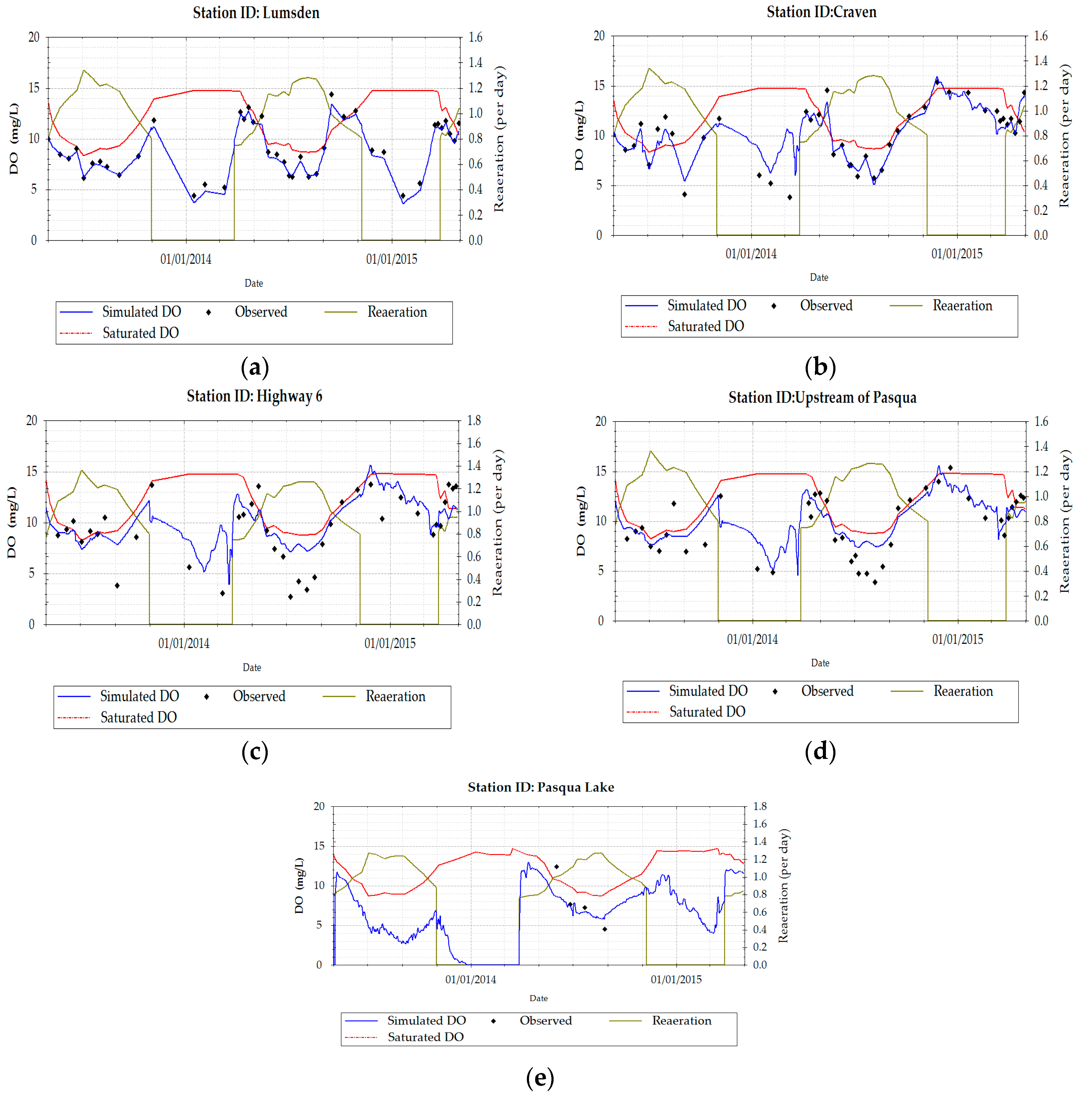
Optimum temporal and spatial SOD rates and temperature correction coefficient values for each segment were calibrated and verified for the periods 1 May 2013 to 30 April 2014 and 1 May 2014 to 30 April 2015 to cover one full summer (May–October) and one full winter (November–April) season in WASP(Athens, GA, USA). Reported SOD rates and temperature correction coefficients for the river and lake systems were varied successively within their reasonable ranges using the Dynamically Dimensioned Search (DDS) algorithm [39] of OSTRICH software (Boston, MA, USA). Optimum rates and coefficients were selected based on how well simulated DO levels matched observed DO levels. The best-fit curves for long-term stations along the river are as shown in Figure 5. Model bias and average prediction errors are shown in Table 1. Mean error (ME) measures the model bias, while mean absolute error (MAE) measures its predictive power. A value of zero ME is usually desired and less than 1.5 mg/L acceptable for variable (DO) prediction. Generally, predicted DO levels were in close agreement with sampled DO at Lumsden, Craven, upstream of Pasqua, and the lakes, but fair agreement was observed for Highway 6. Specifically, the model overpredicted the sampled low DO, especially during the summer season for Highway 6. As the low DO concentration was sampled during periods of high flow (summer time), it is plausible that high levels of diffused loadings from catchments draining into these sites could be occurring. As in-stream sampling data for loading was sparse, this process could not be well represented in the model. Another contributing factor could be the low frequency of DO and temperature observation readings. The model uses a daily time step while sampling was undertaken, monthly, on average. The model, thus, interpolates between the monthly values during the simulation and in so doing, could miss the low DO values.
3.2. Spatial and Seasonal Variation of Sediment Oxygen Demand
Generally, the estimated areal sediment flux at 20 °C ranged from 0.79 to 2.2 g/m2/day across the river-lake system (Table 2). These rates are within reported ranges for rivers and lakes [15,19,20,40,41]. A SOD20 rate of 1.9 and 1.7 g/m2/day were estimated for reaches 1 and 2 (over two-fold increase compared to reach 3). Studies by [42] showed a SOD rate range of 0.17 to 0.33 g/m2/day for the Athabasca River. The authors observed a downward gradient of SOD rate from sites downstream of pulp mill and municipal effluent discharge points. Reaches 1 and 2 form the upstream part of the riverine section of the study site. Algae bloom, siltation, and nutrient export from agricultural land are common phenomena for this part of the study area [43]. Urban effluents from Regina and Moose Jaw are conveyed through this stretch of the river and eventually to the chained lakes. This stretch of the river could be experiencing increased benthic decomposition of settled organic matter from effluent and dead algae. Oxygen is usually consumed faster than it is supplied for locations immediately downstream of point discharges through the oxidation of reduced substances. The SOD20 rate, however, decreases as the effluent travels downstream through reaches 3 and 4 (0.79 and 0.98 g/m2/day) with organic matter mineralization, effluent stabilization, and increasing atmospheric reaeration. Background SOD values, however, influence these amounts [44,45,46]. Steep bank, deep morphology, low velocity, and large sediment surface area may have contributed to the SOD20 rate in the lakes [47]. The steep slopes enhance diffuse organic material loadings (from leaves and plant branches), especially during the summer.
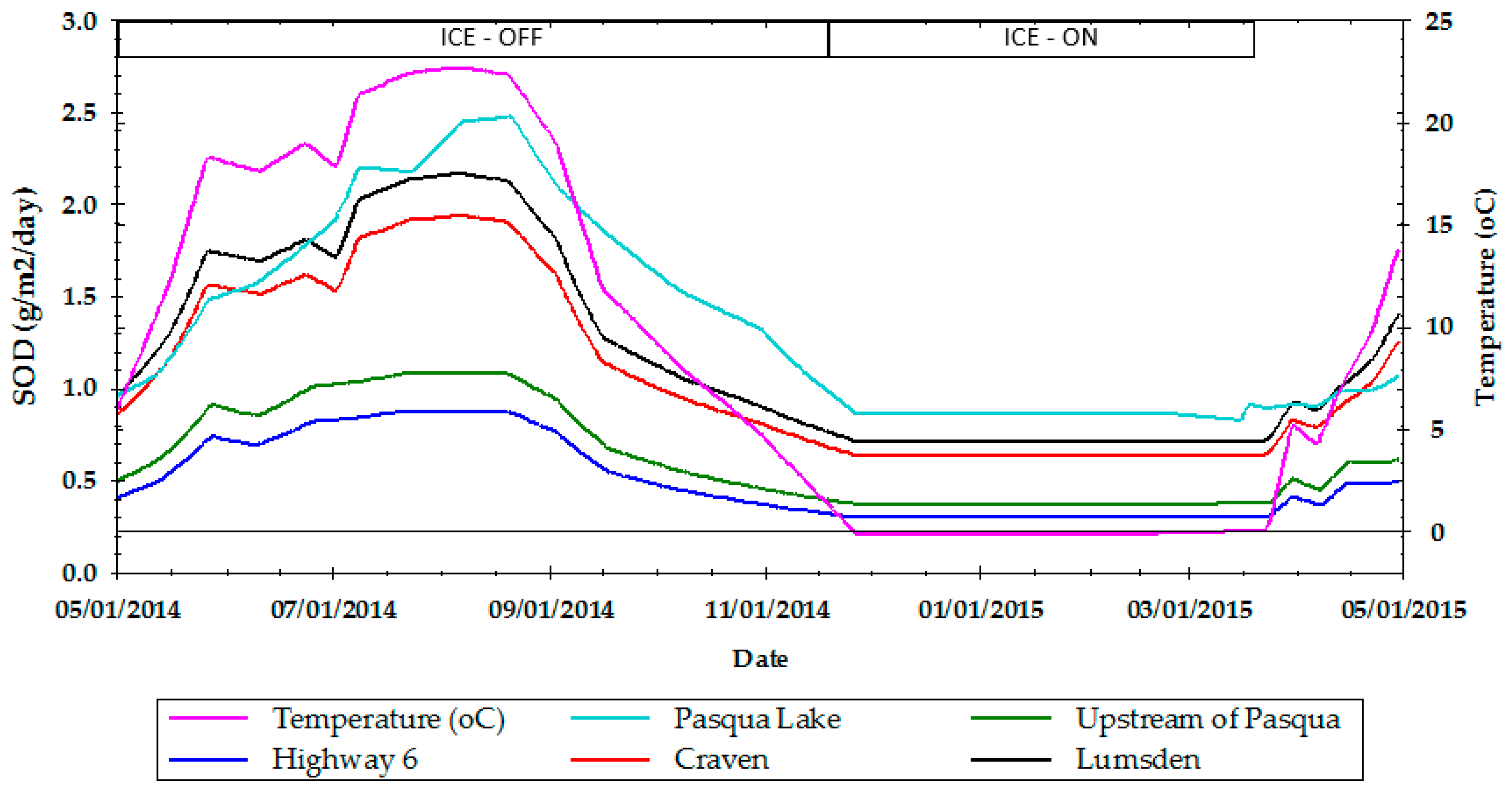
Seasonally, across the system (river and lake), the actual model SOD rates during the simulation period increased steadily after ice-breakup and peaked in the summer but leveling off in the winter (Figure 6). The riverine winter modeled SOD rates ranged from 0.30 to 0.94 g/m2/day. In the lakes, winter SOD rates ranged from 0.83 to 0.95 g/m2/day. In the study by [48], SOD rates for 11 eutrophic ice-covered lakes in Alberta ranged from 0.243 to 0.848 g/m2/day. The higher estimated SOD rates for the Qu’Appelle Lakes may be due to their hypereutrophic nature. The lakes’ SOD rates increased three-fold in the summer compared to the winter and likewise, the river SOD rates increased by a factor of 3. Breakup and summer rainfall often lead to large deposition of sand, debris and allocthonous organic material especially in pool and riffle areas [49]. Hypolimnetic oxygen consumption thus increases as organic matter settles and are oxidized several days after such events.
4. Conclusions
In this study, the SOD rates for a chained river-lake system have been estimated through the calibration of a slightly modified Streeter-Phelps BOD-DO water quality model. Due to the high sampling expenditure, routine sampling of SOD rates are often rare and little is known about the trend in a complex system like a chained river-lake system. River-lake transport and reaeration which influences SOD estimations were calibrated and constrained, respectively. Study results show that SOD20 rates gradually decreased from 1.9 to 0.79 g/m2/day in the riverine section of the system as urban effluent traveled through the river; meanwhile, a SOD20 rate of 2.2 g/m2/day was observed in the lakes. Seasonally, modeled SOD rate increased three-fold in the lakes and the river, respectively, in summer as compared to winter periods. The estimated SOD rates are within reported values of similar studies for rivers and lakes [15,19,20,40,41,42,48]. A downward gradient of SOD was observed in the riverine section of the study site. This trend is attributed to a plausible increase in organic matter decomposition at reaches 1 and 2 and mineralization, effluent stabilization, and increased reaeration in reaches 3 and 4. Studies by [42] for an ice-covered river reported increases in SOD rates for sites immediately downstream of effluent discharge points. Most ice-covered rivers in the world exhibit a linear relationship between oxygen depletion and river distance [51]. The lakes in the study site are shallow. Large sediment surface area, steep banks, and morphology may have contributed to the highly-estimated SOD rate in the lakes. The study by [48] attributed estimated SOD rates for ice-covered lakes in Alberta to a high lake productivity.
Increased bacterial activities in the sediments during the summer and sediment resuspension as a result of high flows may have contributed to the observed higher summer SOD rates in both rivers and lakes.
The zero-order model adopted to estimate the SOD rates in this study is not expected to predict the absolute values of SOD for the river and lakes due to limitations including the mechanism to capture how sediment organic matter converts to sediment oxygen demand [52]. Increasing the model complexity may improve the model results but this has to be accompanied by relevant observations [33] in order to reduce model uncertainties. In situ SOD measurements may be required in the river reaches and lake in the future to further verify the modeled results. Despite these shortcomings, the results are deemed reasonable for water quality modeling purposes of the complex river system in the absence of measured SOD data. The approach adopted in this study is also better than just selecting literature values to run water quality models.
The results of the study provide insights into the SOD rates and seasonal trends, especially for northern rivers.
Acknowledgments
This project was funded by Environment Canada’s Environmental Damages Fund under the project: A water quality modeling system of the Qu’Appelle River catchment for long-term water management policy development.
Author Contributions
Eric Akomeah and Karl-Erich Lindenschmidt conceived and designed the experiments; Eric Akomeah performed the experiments and processed the results; Karl-Erich Lindenschmidt supervised, reviewed, and contributed to the writing of the article.
Conflicts of Interest
Authors declare no conflicts of interest.
References
- Martin, N.; McEachern, P.; Yu, T.; Zhu, D.Z. Model development for prediction and mitigation of dissolved oxygen sags in the Athabasca River, Canada. Sci. Total Environ. 2013, 443, 403–412. [Google Scholar] [CrossRef] [PubMed]
- Zahraeifard, V.; Deng, Z. Modeling sediment resuspension-induced DO variation in fine-grained streams. Sci. Total Environ. 2012, 441, 176–181. [Google Scholar] [CrossRef] [PubMed]
- Liu, W. Measurement of sediment oxygen demand for modelling dissolved oxygen distribution in tidal Keelung River. Water Environ. J. 2009, 23, 100–109. [Google Scholar] [CrossRef]
- Tian, Y. A Dissolved Oxygen Model and Sediment Oxygen Demand Study in the Athabasca River. Master’s Thesis, University of Alberta, Edmonton, AB, Canada, 2005. [Google Scholar]
- MacPherson, T.A. Sediment Oxygen Demand and Biochemical Oxygen Demand: Patterns of Oxygen Depletion in Tidal Creek Sites. Master’s Thesis, University of North Carolina Wilmington, Wilmington, NC, USA, 2003. [Google Scholar]
- Rounds, S.; Doyle, M.C. Sediment Oxygen Demand in the Tualatin River Basin, Oregon, 1992–1996; US Department of the Interior, US Geological Survey: Porland, OR, USA, 1997.
- MacPherson, T.A.; Cahoon, L.B.; Mallin, M.A. Water column oxygen demand and sediment oxygen flux: Patterns of oxygen depletion in tidal creeks. Hydrobiologia 2007, 586, 235–248. [Google Scholar] [CrossRef]
- Hu, W.; Lo, W.; Chua, H.; Sin, S.; Yu, P. Nutrient release and sediment oxygen demand in a eutrophic land-locked embayment in Hong Kong. Environ. Int. 2001, 26, 369–375. [Google Scholar] [CrossRef]
- Matlock, M.D.; Kasprzak, K.R.; Osborn, G.S. Sediment oxygen demand in the Arroyo Colorado River. JAWRA J. Am. Water Resour. Assoc. 2003, 39, 267–275. [Google Scholar] [CrossRef]
- Higashino, M.; Gantzer, C.J.; Stefan, H.G. Unsteady diffusional mass transfer at the sediment/water interface: Theory and significance for SOD measurement. Water Res. 2004, 38, 1–12. [Google Scholar] [CrossRef] [PubMed]
- Haag, I.; Schmid, G.; Westrich, B. Dissolved Oxygen, and Nutrient Fluxes across the Sediment–Water Interface of the Neckar River, Germany: In Situ Measurements and Simulations. Water Air Soil Pollut. Focus 2006, 6, 413–422. [Google Scholar] [CrossRef]
- Diaz, R.J.; Rosenberg, R. Spreading Dead Zones and Consequences for Marine Ecosystems. Science 2008, 321, 926–929. [Google Scholar] [CrossRef] [PubMed]
- Chau, K. Field measurements of SOD and sediment nutrient fluxes in a land-locked embayment in Hong Kong. Adv. Environ. Res. 2002, 6, 135–142. [Google Scholar] [CrossRef]
- Rasheed, M.; Al-Rousan, S.; Manasrah, R.; Al-Horani, F. Nutrient fluxes from deep sediment support nutrient budget in the oligotrophic waters of the Gulf of Aqaba. J. Oceanogr. 2006, 62, 83–89. [Google Scholar] [CrossRef]
- Miskewitz, R.J.; Francisco, K.L.; Uchrin, C.G. Comparison of a novel profile method to standard chamber methods for measurement of sediment oxygen demand. J. Environ. Sci. Health Part A 2010, 45, 795–802. [Google Scholar] [CrossRef] [PubMed]
- Zeledon-Kelly, R.V. Effects of Landuse on Sediment Oxygen Demand for Streams in Northwest Arkansas and the Validation of a Sediment Oxygen Demand Measure-Plus-Calculate Model; ProQuest: Fayetteville, AR, USA, 2009. [Google Scholar]
- McDonnell, A.J.; Hall, S.D. Effect of environmental factors on benthal oxygen uptake. J. Water Pollut. Control Fed. 1969, 41, R353–R363. [Google Scholar]
- Mackenthun, A.A.; Stefan, H.G. Effect of flow velocity on sediment oxygen demand: Experiments. J. Environ. Eng. 1998, 124, 222–230. [Google Scholar] [CrossRef]
- Liu, W.; Chen, W. Monitoring sediment oxygen demand for assessment of dissolved oxygen distribution in river. Environ. Monit. Assess. 2012, 184, 5589–5599. [Google Scholar] [CrossRef] [PubMed]
- Caldwell, J.M.; Doyle, M.C. Sediment Oxygen Demand in the Lower Willamette River, Oregon; Water-Resources Investigations Report; U.S. Geological Survey: Portland, OR, USA, 1995.
- Paraska, D.W.; Hipsey, M.R.; Salmon, S.U. Sediment diagenesis models: Review of approaches, challenges and opportunities. Environ. Model. Softw. 2014, 61, 297–325. [Google Scholar] [CrossRef]
- Massoudieh, A.; Bombardelli, F.; Ginn, T.; Green, P.; Ferreira, R. Mathematical modeling of the biogeochemistry of dissolved and sediment-associated trace metal contaminants in riverine systems. In Proceedings of the International Conference on Fluvial Hydraulics, Lisbon, Portugal, 6–8 September 2006. [Google Scholar]
- Sohma, A.; Sekiguchi, Y.; Yamada, H.; Sato, T.; Nakata, K. A new coastal marine ecosystem model study coupled with hydrodynamics and tidal flat ecosystem effect. Mar. Pollut. Bull. 2001, 43, 187–208. [Google Scholar] [CrossRef] [PubMed]
- Sohma, A.; Sekiguchi, Y.; Nakata, K. Modeling and evaluating the ecosystem of sea-grass beds, shallow waters without sea-grass, and an oxygen-depleted offshore area. J. Mar. Syst. 2004, 45, 105–142. [Google Scholar] [CrossRef]
- Sohma, A.; Sekiguchi, Y.; Kuwae, T.; Nakamura, Y. A benthic–pelagic coupled ecosystem model to estimate the hypoxic estuary including tidal flat—Model description and validation of seasonal/daily dynamics. Ecol. Model. 2008, 215, 10–39. [Google Scholar] [CrossRef]
- Gualtieri, C. Sediment oxygen demand modeling in dissolved oxygen balance. In Proceedings of the International Conference on Environmental engineering and renewable energy, Ulaanbaatar, Mongolia, 7–10 September 1998. [Google Scholar]
- Slama, C.A. Sediment oxygen Demand and Sediment Nutrient Content of Reclaimed Wetlands in the Oil Sands Region of Northeastern Alberta. Master’s Thesis, University of Windsor, Windsor, ON, Canada, 2010. [Google Scholar]
- Boudreau, B.P. A method-of-lines code for carbon and nutrient diagenesis in aquatic sediments. Comput. Geosci. 1996, 22, 479–496. [Google Scholar] [CrossRef]
- Meysman, F.J.; Middelburg, J.J.; Herman, P.M.; Heip, C.H. Reactive transport in surface sediments. I. Model complexity and software quality. Comput. Geosci. 2003, 29, 291–300. [Google Scholar] [CrossRef]
- Bierman, V., Jr.; DePinto, J.; Dilks, D.; Moskus, P.; Slawecki, T.; Bell, C.; Chapra, S.; Flynn, K. Modeling Guidance for Developing Site-Specific Nutrient Goals; Water Environment Research Foundation: Alexandria, VA, USA, 2013. [Google Scholar]
- Wool, T.A.; Ambrose, R.B.; Martin, J.L.; Comer, E.A.; Tech, T. Water Quality Analysis Simulation Program (WASP). User’s Manual; U.S Environmental Protection Agency, Center for Exposure Assessment Modeling: Athens, GA, USA, 2006.
- Terry, J.A.; Sadeghian, A.; Lindenschmidt, K. Modelling Dissolved Oxygen/Sediment Oxygen Demand under Ice in a Shallow Eutrophic Prairie Reservoir. Water 2017, 9, 131. [Google Scholar] [CrossRef]
- Cox, L.A. Internal dose, uncertainty analysis, and complexity of risk models. Environ. Int. 1999, 25, 841–852. [Google Scholar] [CrossRef]
- Quinlan, R.; Leavitt, P.R.; Dixit, A.S.; Hall, R.I.; Smol, J.P. Landscape effects of climate, agriculture, and urbanization on benthic invertebrate communities of Canadian prairie lakes. Limnol. Oceanogr. 2002, 47, 378–391. [Google Scholar] [CrossRef]
- Hall, R.I.; Leavitt, P.R.; Quinlan, R.; Dixit, A.S.; Smol, J.P. Effects of agriculture, urbanization, and climate on water quality in the northern Great Plains. Limnol. Oceanogr. 1999, 44, 739–756. [Google Scholar] [CrossRef]
- United States Army Corps of Engineers, Hydrologic Engineering Center. HEC-RAS River Analysis System 2D Modelling User’s Manual Version 5.0; Hydrologic Engineering Center, United States Corps of Engineer: Davis, CA, USA, 2016. [Google Scholar]
- Ambrose, R.; Wool, T. WASP7 Stream Transport-Model Theory, and User’s Guide, Supplement to Water Quality Analysis Simulation Program (WASP) User Documentation; National Exposure Research Laboratory, Office of Research and Development, US Environmental Protection Agency: Athens, GA, USA, 2009.
- Akomeah, E.; Chun, K.P.; Lindenschmidt, K. Dynamic water quality modelling and uncertainty analysis of phytoplankton and nutrient cycles for the upper South Saskatchewan River. Environ. Sci. Pollut. Res. 2015, 22, 18239–18251. [Google Scholar] [CrossRef] [PubMed]
- Tolson, B.A.; Shoemaker, C.A. Dynamically dimensioned search algorithm for computationally efficient watershed model calibration. Water Resour. Res. 2007, 43, 208–214. [Google Scholar] [CrossRef]
- Chiaro, P.S.; Burke, D.A. Sediment oxygen demand and nutrient release. In Conference on Environmental Engineering: Research Development and Design, Proceedings of the Environmental Engineering Division Specialty Conference, Kansas City, MO, USA, 10–12 July 1978; American Society of Civil Engineers: Kansas City, MO, USA, 1978; pp. 313–322. [Google Scholar]
- James, A. The measurement of benthal respiration. Water Res. 1974, 8, 955–959. [Google Scholar] [CrossRef]
- Zhu, D.; Yu, T. Spatial variation of sediment oxygen demand in Athabasca River: Influence of water column pollutants. In Proceedings of the World Environmental and Water Resources Congress, Kansas City, MO, USA, 17–21 May 2009; pp. 1–12. [Google Scholar]
- Clifton Associates Ltd. Upper Qu’Appelle Water Supply Project: Economic Impact and Sensitivity Analysis; Water Security Agency: Regina, SK, Canada, 2012. [Google Scholar]
- McCulloch, J.; Gudimov, A.; Arhonditsis, G.; Chesnyuk, A.; Dittrich, M. Dynamics of P-binding forms in sediments of a mesotrophic hard-water lake: Insights from non-steady state reactive-transport modeling, sensitivity and identifiability analysis. Chem. Geol. 2013, 354, 216–232. [Google Scholar] [CrossRef]
- Maerki, M.; Müller, B.; Wehrli, B. Microscale mineralization pathways in surface sediments: A chemical sensor study in Lake Baikal. Limnol. Oceanogr. 2006, 51, 1342–1354. [Google Scholar] [CrossRef]
- United States Environmental Protection Agency. Technical Guidance Manual for Developing Total Maximum Daily Loads, Book 2: Streams and Rivers, Part 1: Biochemical Oxygen Demand and Nutrients/Eutrophication; U.S. EPA: Washington, DC, USA, 1995.
- Blais, J.M.; Kalff, J. The influence of Lake Morphometry on sediment focusing. Limnol. Oceanogr. 1995, 40, 582–588. [Google Scholar] [CrossRef]
- Babin, J.; Prepas, E. Modelling winter oxygen depletion rates in ice-covered temperate zone lakes in Canada. Can. J. Fish. Aquat. Sci. 1985, 42, 239–249. [Google Scholar] [CrossRef]
- Elwood, J.W.; Waters, T.F. Effects of floods on food consumption and production rates of a stream brook trout population. Trans. Am. Fish. Soc. 1969, 98, 253–262. [Google Scholar] [CrossRef]
- Thomann, R.V.; Mueller, J.A. Principles of Surface Water Quality Modeling and Control; Harper & Row: New York, NY, USA, 1987. [Google Scholar]
- Chambers, P.; Scrimgeour, G.; Pietroniro, A. Winter oxygen conditions in ice-covered rivers: The impact of pulp mill and municipal effluents. Can. J. Fish. Aquat. Sci. 1997, 54, 2796–2806. [Google Scholar] [CrossRef]
- Chapra, S.C. Surface Water-Quality Modeling; Waveland Press: Long Grove, IL, USA, 2008. [Google Scholar]
Figure 1.
Map of the Qu’Appelle River System.

Figure 2.
Monthly mean flow at WSC gauge 05JF001, Lumsden, from 1911 to 2016.

Figure 3.
Ice freeze-up (left) and break-up (right) conditions at the Elbow River gauge between 1970 and 2010.
Figure 3.
Ice freeze-up (left) and break-up (right) conditions at the Elbow River gauge between 1970 and 2010.
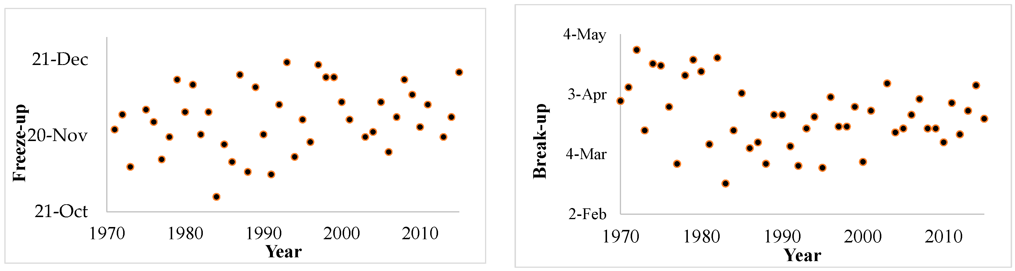
Figure 4.
Longitudinal profile showing modeled surface water elevation (blue line), observed stage (red diamond square), and river thalweg (black line).
Figure 4.
Longitudinal profile showing modeled surface water elevation (blue line), observed stage (red diamond square), and river thalweg (black line).
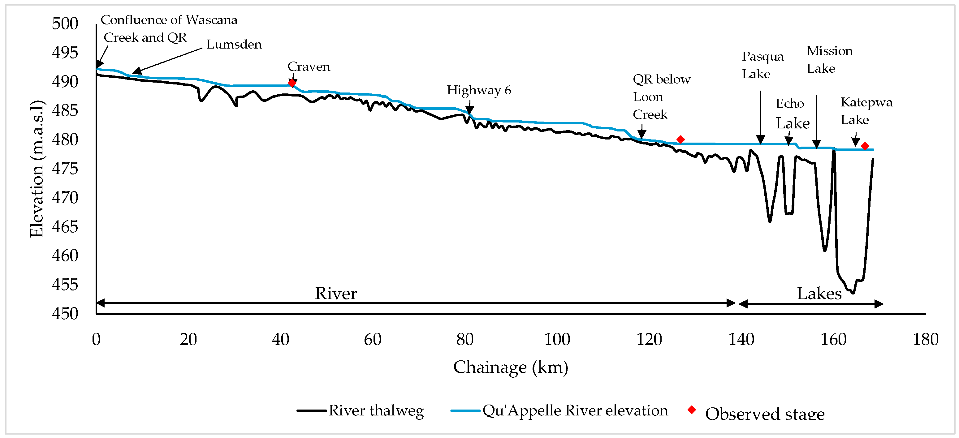
Figure 5.
Simulated and sampled dissolved oxygen for the calibration and validation periods: the left and right vertical axes represent dissolved oxygen and reaeration coefficient, respectively; from the upstream of the study area, (a) Lumsden; (b) Craven; (c) Highway 6; (d) upstream of Pasqua Lake; and (e) Pasqua lake.

Figure 6.
Seasonal variation of SOD rate in the QR system (these rates are model-based results and not normalized to 20 °C).
Figure 6.
Seasonal variation of SOD rate in the QR system (these rates are model-based results and not normalized to 20 °C).


Table 1.
Model bias and prediction error.
| Gauge Station | Mean Error | Mean Absolute Error |
|---|---|---|
| Lumsden | −0.32 | 0.35 |
| Craven | −0.03 | 0.77 |
| Highway 6 | 0.62 | 1.78 |
| Upstream of Pasqua | 0.36 | 1.36 |
| Pasqua | −0.62 | 1.30 |
Table 2.
Calculated Model Segment SOD rates and temperature correction coefficient 1.
| River Reach/Lake | Description | Optimum SOD (g/m2/Day) at 20 °C | Reported SOD Range | Reference |
|---|---|---|---|---|
| Reach 1 | Wascana-QR confluence to Lumsden | 1.90 | (0.1–5.3) (SOD) | [40] 2 |
| (1.04–1.13) (Temp. coefficient) | [50] | |||
| Reach 2 | Lumsden to Craven | 1.70 | (0.1–5.3) | [40] |
| Reach 3 | Craven to Highway 6 | 0.79 | (0.1–5.3) | [40] |
| Reach 4 | Highway 6 to Qu’Appelle below Loon Creek | 0.98 | (0.1–5.3) | [40] |
| Lakes | Pasqua, Echo Mission, Katepwa lakes | 2.20 | (0.7–8.4) | [41] 3 |
Notes: 1 The model was calibrated to an optimum temperature coefficient of 1.05 for all reaches and lakes; 2 The reported range represents SOD measurements between 19 and 25 °C for six Eastern Michigan river stations; 3 Oxygen mass balance for lakes.
© 2017 by the authors. Licensee MDPI, Basel, Switzerland. This article is an open access article distributed under the terms and conditions of the Creative Commons Attribution (CC BY) license (http://creativecommons.org/licenses/by/4.0/).
Share and Cite
MDPI and ACS Style
Akomeah, E.; Lindenschmidt, K.-E. Seasonal Variation in Sediment Oxygen Demand in a Northern Chained River-Lake System. Water 2017, 9, 254. https://doi.org/10.3390/w9040254
AMA Style
Akomeah E, Lindenschmidt K-E. Seasonal Variation in Sediment Oxygen Demand in a Northern Chained River-Lake System. Water. 2017; 9(4):254. https://doi.org/10.3390/w9040254
Chicago/Turabian StyleAkomeah, Eric, and Karl-Erich Lindenschmidt. 2017. "Seasonal Variation in Sediment Oxygen Demand in a Northern Chained River-Lake System" Water 9, no. 4: 254. https://doi.org/10.3390/w9040254
Note that from the first issue of 2016, this journal uses article numbers instead of page numbers. See further details here.