
Comparative Analysis of HRU and Grid-Based SWAT Models


1
Department of Agricultural and Biological Engineering, Purdue University, West Lafayette, IN 47907, USA
2
Stone Environmental, Montpelier, VT 05602, USA
3
Department of Agricultural and Biological Engineering, Pennsylvania State University, University Park, PA 16802, USA
4
Department of Earth, Atmospheric, and Planetary Sciences, Purdue University, West Lafayette, IN 47907, USA
5
Lyles School of Civil Engineering, Purdue University, West Lafayette, IN 47907, USA
*
Author to whom correspondence should be addressed.
Water 2017, 9(4), 272; https://doi.org/10.3390/w9040272
Submission received: 6 February 2017
/
Revised: 23 March 2017
/
Accepted: 6 April 2017
/
Published: 12 April 2017
Abstract
:A grid-based version of the Soil and Water Assessment Tool (SWAT) model, SWATgrid, was developed to perform simulations on a regularized grid with a modified routing algorithm to allow interaction between grid cells. However, SWATgrid remains largely untested with little understanding of the impact of user-defined grid cell size. Moreover, increases in computation time effectively preclude direct calibration of SWATgrid. To gain insight into defining appropriate strategies for future development and application of SWATgrid, this research considers the simulated differences between commonly-employed hydrologic response unit (HRU)-based and grid-based SWAT models and the implications of resolution on their simulation and calibrated parameter values for a Midwestern, agricultural watershed. Results indicate that: (1) the gridded approach underpredicted simulated streamflow between 5% and 50% relative to the baseline model, depending upon the input spatial resolution and routing algorithm implemented; (2) gridded models generally underpredicted total phosphorous and sediment loads while overpredicting nitrate load; and (3) ranges of values of optimized model parameters remained similar up to 90 m. Results from this analysis should help in defining future applications of the SWATgrid model and the effects of differing spatial resolution of the model input data.
1. Introduction
A critical repercussion of agroecosystem growth is the deterioration of water quality from nonpoint source pollution derived from locations that cannot be ascribed spatially in the landscape [1]. Transport of nitrogen (N) and phosphorous (P) [2,3,4], sediment [5] and pesticides [6] is responsible for a range of adverse impacts on human and environmental conditions [7], constituting the primary source for impairment of rivers and streams in the United States [8]. Given the difficulty in identifying and controlling nonpoint source pollution, traditional monitoring and regulatory strategies, such as point-based monitoring, are difficult. Further, attempts to test possible management solutions are encumbered by cost, uncertainty and potential lack of participation.
Hydrologic models provide the capability to represent and predict natural processes, especially where observations are limited, thereby aiding in scenario analysis of system response to the implementation of nonpoint source control measures. Accordingly, there is a need to understand the accuracy and fidelity of these models in representing known processes to improve the predictive certainty for a range of intended applications. Uncertainty in hydrologic models is attributed to a combination of measurement error, systematic error, natural variation, model uncertainty, subjective judgement and inherent randomness [9,10,11]. Therefore, efforts to improve the capability of hydrologic models to effectively capture and mathematically represent natural processes in a physically meaningful way necessitates continuing adaptation and refinement of methodology.
River basins and watersheds are common boundaries of most hydrologic models focused on nonpoint source pollution, as they provide an integrated response of natural and anthropogenic processes [12]. Reviews of several hydrologic models underscore differences in the choice of discretization and model complexity to capture system response [13,14,15]. Mathematical representation of physical processes depends on the level of discretization used and should reflect the scale of interest of the intended application. Discretization can be defined either temporally or spatially and seeks to relate the modeled scale to observation and process scales [16]. Changes in scale may require development of new mathematical models and approaches. Based on data availability, hydrologic models generally adopt a daily time step, although effects of temporal scale are not well understood [17]. Simple, lumped approaches often are appropriate spatially and can produce comparable results to more detailed, complex approaches depending upon the application [18,19]. However, many simple hydrologic models lack necessary physical processes and management scenarios essential for modeling the associated transformation and transport of nonpoint source pollution [12]. Balancing the need for explicitly modeling spatial processes with data availability and computational cost is thus an ongoing research issue [20]. Calibration of the model is of equal importance, as it may contribute to improved results or may mask deficiencies in simulations [21].
The Soil and Water Assessment Tool (SWAT) is a continuous-time, distributed-parameter model, capable of simulating hydrology and water quality at the watershed scale [22]. According to Wellen et al. [15], SWAT is the most commonly-used model for distributed watershed nutrient modeling and has been used in a wide range of applications [23]. SWAT predominantly relies upon discretizing landscapes based on common soil, land use and slope characteristics, known as hydrologic response units (HRUs). While the HRU approach provides a simple, computationally-efficient framework, processes modeled on HRUs are lumped and therefore spatially disconnected, as they are routed directly to subbasin outlets. This was identified as a key weakness of the model by Gassman [23] and Douglas-Mankin et al. [24], among others. This lack of definition of landscape position makes implementation of spatially-targeted management difficult to incorporate in the model.
Although readily accessible in the SWAT model framework, few studies have evaluated modified discretization or routing beyond standard HRU routing through subbasin networks [20,25,26,27,28]. To overcome the spatial limitations of the HRU approach, a grid-based version of the SWAT model, SWATgrid [29], was developed to perform landscape simulation on a regularized grid [30] and employ a modified landscape routing algorithm developed by Volk et al. [31] and Arnold et al. [20] to spatially connect grids during routing. While other gridded hydrologic models exist, few incorporate detailed management, plant growth and water quality algorithms intrinsic to SWAT.
Rathjens et al. [29] found the approach was able to simulate streamflow reasonably well. However, SWATgrid remains largely untested, with little understanding of the impact of user-defined model spatial resolution. Previous studies have been conducted at spatial resolutions of 100 m or greater and have not considered watersheds with artificially drained by subsurface tiles ubiquitous to poorly-drained agricultural landscape, such as the U.S. Midwestern agricultural systems [29,30,32]. Unfortunately, computational overhead is significant for SWATgrid, effectively precluding direct calibration and necessitating strategies such as parameter transfer from HRU-based SWAT models [33]. Parameters have been shown to exhibit scale dependency [34], so correct characterization of their distributions at various resolutions is critical prior to transfer.
Use of subbasins is the most commonly-employed spatial discretization approach in watershed modeling [15]; however, input data are generally initially available in gridded raster format prior to reconceptualization. Typical spatial input data include a digital elevation model (DEM), land use and soils. For hydrologic modeling, modifying the resolution of a DEM is considered the most impactful as it affects watershed delineation, slopes and channel length, while land use and soil classification primarily modify flow partitioning [35]. Several studies have assessed the impact of DEM resolution on hydrology and water quality predictions with SWAT. Runoff, sediment and nutrients were found to decrease with coarser resolution by Cho and Lee [36], Chaubey et al. [37] and Ghaffari et al. [38], due to smoothing of average watershed slope. Conversely, Chaplot [39], Lin et al. [40], Shen et al. [41] and Zhang et al. [42] identified minimal change in flow while water quality variables remained impacted.
Research focused on the impacts of resolution on SWAT has not yet extended beyond the standard HRU-based approach. The overall goal of this study was to test the efficacy of the SWATgrid approach while gaining insight into its sensitivity to user-defined spatial input resolution. Accordingly, three objectives were considered: (1) identifying a target resolution range for SWATgrid applications to maximize predictive accuracy while minimizing computation time; (2) comparing SWATgrid simulations to HRU simulations; and (3) identifying differences in calibrated parameter ranges for varying resolutions. Future SWAT applications, such as identifying critical source areas or testing best management practices, may require greater spatial detail [43] than afforded by subbasin discretization. The grid-based approach offers one possibility to capture such spatial details in order to develop effective land management options for reducing losses of nonpoint source pollutants.
2. Materials and Methods
To accomplish the objectives of this study, several models were created using multiple input data resolutions for both the SWAT and SWATgrid. SWAT HRU models used the standard SWAT routing methods, while SWATgrid models (GRID) implemented both standard and landscape routing. This enabled a more rigorous comparison of HRU- and GRID-based methodologies by isolating both the effects of the landscape routing and, in turn, the gridded spatial representation of the landscape. Therefore, for each resolution considered, three separate model simulations were assessed: (1) HRU-based spatial representation with standard routing (HRU); (2) GRID-based spatial representation with landscape routing (GRID-LAND or LAND); and (3) GRID-based spatial representation with standard routing (GRID-STD or STD).
2.1. Study Location
The Cedar Creek Watershed (CCW) is located in the southwestern region of the St. Joseph River Basin in northeastern Indiana. Covering approximately 707 km2, the CCW drains two HUC (Hydrologic Unit Code) 10 subwatersheds (0410000306 and 0410000307). A monitoring network was established in the northern CCW subbasin in 2002 as part of the United States Department of Agriculture’s Agricultural Research Service’s (USDA-ARS) Source Water Protection Project (SWPP) and Conservation Effect Assessment Project (CEAP), and it is shown in Figure 1. The topography is characterized by slopes of 2% to 10% with an overall gradient towards the southeastern outlet. Soils were formed from compacted glacial till and fluvial materials with silt loam, silty clay loam and clay loam textures. The CCW is primarily agricultural, with corn and soybean rotational planting, although winter wheat, oats, alfalfa and pasture are also present [44,45,46]. Due to oversaturation of soils and the prevalence of agricultural land, tile drainage is commonly employed throughout the watershed. Climatic conditions for the CCW include historical average temperatures from −1 to 28 °C with 940 mm of annual precipitation. For this study, two weather stations were used, one in the lower center of the watershed and a second outside the watershed boundary to the north. Station data were obtained from the USDA SWAT climate dataset <ars.usda.gov/Research/docs.htm?docid=19388>.
2.2. The SWAT Model
The SWAT model is a continuous-time, semi-distributed, process-based river basin model [22]. Inclusion of hydrology, weather, crop growth, soil, nutrient, pesticide and agricultural management components allows SWAT to predict the impact of various agricultural management scenarios on hydrology and water quality. Fundamentally, the model is hydrologically driven, based upon the water balance of an individual landscape unit:
where SW is the soil water content, R is precipitation, Q is surface runoff, ET is evapotranspiration, P is percolation and QR is return flow in units of mm for each day, i. Each landscape unit consists of a possible snow layer, a soil profile divided into multiple layers and a shallow and deep aquifer.
Standard SWAT Routing
Hydrologic processes are first simulated at the landscape (HRU) level and subsequently routed at the subbasin level where each subbasin has an associated reach. Landscape discretization into HRUs provides a simple framework for simulation, but also represents a significant limitation of the model. Spatial connectivity and interactions among HRUs are ignored, instead aggregating the cumulative output of each spatially discontinuous HRU group at the subwatershed outlet, which is then directly routed to the channel. Water balance equations are applied at the HRU level. For complete documentation, see Neitsch et al. [47].
2.3. SWATgrid
SWATgrid differs from HRU-based SWAT models in two key ways: (1) use of gridded, discretized landscape units and (2) linking these landscape unit grids and routing surface runoff, lateral subsurface and shallow groundwater flow. Gridded landscape units effectively function as both an HRU and subbasin and take advantage of standard SWAT landscape simulation algorithms.
As part of SWATgrid, Rathjens and Oppelt [30] developed an approach that utilizes the Topographic Parameterization (TOPAZ [48]) tool to generate gridded landscape units. The grids allow for spatial connectivity during the routing phase as they are at a defined location, as opposed to HRUs, which are not. Landscape routing is then implemented through these grids adapted from the approach used by Volk et al. [31] and Arnold et al. [20]. Spatial position for each grid is calculated from a modified topographic index adapted from the TOPMODEL (Topography Based Hydrologic Model) framework:
where Ai is the upslope contributing area per unit contour length (m), βi is the topographic slope angle, Ki is mean saturated hydraulic conductivity (m/day) and Zi is the soil depth (m) for each grid cell i. As the index approaches one, it approximates a valley or floodplain and near zero, a divide. Effectively, the index partitions flow on a given grid cell between channelized and landscape flow. In SWATgrid, the flow separation index is normalized for either abrupt or gradual channel heads and is adjusted by the drainage density of the watershed to capture channel head locations more accurately. Thus, when the adjusted flow separation index is zero, there is only landscape flow, and conversely when it is one, the flow is completely channelized. For an in-depth description of the SWATgrid, see Rathjens et al. [29].
2.4. Baseline Model
An initial 30-m spatial resolution model was developed and calibrated to serve as a baseline for comparison of model simulations across resolutions. The 30-m resolution was nominally selected as the finest scale considered, given that it is common for most spatial datasets used in SWAT modeling (e.g., National Elevation Data (NED), National Land Cover Database (NLCD)). The watershed was delineated using a 30-m digital elevation model (DEM) from the NED. Land use and soil properties were obtained from the Crop Data Layer (CDL, 2010) from the National Agricultural Statistics Service (NASS) at 30 m and State Soil Geographic (STATSGO) Dataset at 250 m, respectively. STATSGO data were selected given their native grid structure provided by the SWAT soils database and relatively fewer soil classes than other soil databases (e.g., SSURGO—Soil Survey Geographic Database) , which facilitate ease of writing the manually intensive SWATgrid input files. STATSGO data were resampled by the nearest neighbor approach to 30 m prior to rescaling at coarser resolutions. Various CDL agricultural land use categories constituting less than 1% of the watershed area (e.g., pumpkins) were reclassified to general agriculture.
The model was forced with precipitation and temperature data from 1990 to 2010 from the United States Department of Agriculture (USDA) Agricultural Research Service (ARS) SWAT U.S. Climate Dataset stations C120200 and C123207. Discharge data for calibration and validation at the watershed outlet were obtained from the United States Geological Survey (USGS) Water Data Server for Station Number 04180000, Cedar Creek near Cedarville, IN, over the same period. Geographic input datasets are shown in Figure 1.
Delineation and initial model parameterization were achieved using the ArcSWAT interface with the input datasets previously described. Based on previous experience in modeling this watershed, 1000 ha were used to define the minimum area necessary for channel formation. As SWATgrid evaluates all unique possible combinations of land use and soil types in the model, the HRU threshold for soils and land use was set to 0%. Watershed delineation produced 43 subbasins consisting of 1082 HRUs.
Several initial parameters values were specified in accordance with previous research in similar agricultural watersheds, as well as using expert knowledge, including previously published SWAT modeling studies from this area. Management parameters were specified to fit dominant expected scenarios for a corn and soybean rotation, as shown in Table 1 (see [49] for details). Additionally, given the prominence of tile drained agricultural landscapes in the Midwest [50], tile drainage was implemented in each HRU comprised of a corn-soybean rotation located on poorly- or very poorly-drained soils (soil hydrologic Groups C and D, respectively). The modifications required for tile drains are summarized in Table 2 (see [51] for details). Additionally, to allow water to drain into the tiles, the curve number parameters were adjusted by assuming that each C or D class soil would behave as one class above its level. Finally, the SWAT baseflow recession constant (ALPHA_BF) was estimated using the SWAT Baseflow Filter Program [52,53] and set to 0.0321.
Based on previous SWAT research in Northern Indiana [54], six basin level parameters, summarized in Table 3, were specified for model calibration. By selecting basin level, rather than distributed parameters, calibration was applied in a consistent way to all models, regardless of varying HRU relative area between different resolutions and model types. A multi-algorithm, genetically adaptive multi-objective method (AMALGAM) [55] was adapted for use with SWAT input and output data structure. Calibration was performed with monthly simulations between 1990 and 2010. The first four years were used for model warm up, while 1994 to 2003 and 2004 to 2010 were used for calibration and validation. Five thousand simulations were sampled and evaluated over 50 generations. Parameter optimization was constrained by maximizing Nash–Sutcliffe efficiency (NSE [56]).
2.5. Resampling Approach
The SWATgrid model was run at spatial resolutions of 30, 60, 90, 150, 250, 500 and 1000 m. Resolution of the input data has numerous implications in watershed simulations. However, the primary focus here is to select a scale that captures a realistic system response while achieving viable computational time, rather than extensively evaluate the implications of the spatial detail of input data. Land use, soil and topography data were resampled from 30-m base data for each set of conditions. Nearest neighbor resampling was used to preserve the “hard” classes of land use and soils. Similar to other research [57,58], resampling was achieved by bicubic convolution to provide a smoothly interpolated DEM that retains peaks and depressions in the dataset, which is critical in watershed delineation and channel definition. Resampled soil and land use data in the Cedar Creek Watershed had a <2% difference in proportional watershed area between the finest and coarsest resolutions for all classes, even though actual area changed across resolutions.
2.6. Simulation Effects
Input data at 30-m resolution were used to create a baseline SWAT model and calibrated as previously described. Parameters from this baseline model were then transferred to lower resolution HRU and GRID models. By maintaining a constant parameter set applied at the basin level, the effects of resolution and routing type were better isolated. Each HRU and GRID model at 30, 60, 90, 150, 250, 500 and 1000 m (14 total) was run during the same period used for the 30-m baseline model calibration. The same SWAT version (Ver. 574) was used for both HRU and GRID models. HRU models were only run with standard routing, while GRID models were simulated twice, once with landscape routing and once with standard routing used in HRU-based delineation.
Predictive uncertainty derived from varying the input data resolution and model type was based on relative error (RE):
where Simbase is the simulated value from the calibrated, baseline model and Simi,j is the simulated value from the coarsened dataset of resolution i (30, 60, 90 m, …) and model j (HRU, GRID-STD, GRID-LAND). Simulated values refer to flow at the watershed outlet. A baseline model was used rather than USGS-measured streamflow to focus the analysis on differences between the modeling approaches.
2.7. Calibration Effects
Given the significant computation time required by the GRID models, the calibration procedures involved calibrating a standard SWAT HRU-based model and transferring the parameters [33]. As SWATgrid resolution is user defined, it is important to understand the effect of modifying input resolution on calibrated parameter values. Therefore, for the six basin-level parameters used for calibration, HRU models were calibrated individually at all tested resolutions, and resulting parameter values were compared over the final 1000 simulations using the same calibration approach described for the baseline model.
3. Results and Discussion
3.1. Baseline Model Calibration
Summary statistics are shown in Table 4 for the calibration of six parameters using an adapted AMALGAM code for SWAT. The 30-m baseline model was run 5000 times; however, parameters and the optimized objective function value began to converge after approximately 2000 simulations. While several calibrated parameter sets produced equally acceptable results relative to the objective function, known as equifinality [59], the mean of the parameters of the last 100 simulations was selected for calibration.
Applying this parameter set to the model generated a similar monthly flow at the outlet when compared to measured discharge. The hydrographs in Figure 2 illustrate this correspondence and further highlight the temporal congruity of the observed and simulated flow. There are periods of both over- and under-estimation of flow during both high and low flow events. Monthly NSE was 0.8 for both the calibration (1994 to 2003) and validation (2004 to 2010) periods and was considered satisfactory. Similarly, mean simulated and observed flows were in agreement with a slight underprediction in mean flow by the model.
3.2. Watershed Delineation
Watershed boundaries differed as a function of both the delineation method (ArcSWAT vs. TOPAZ) and resolution. In general, watershed area tended to decrease with a coarsening of grid size over the range of resolutions considered; however, the decrease was not consistent over all steps, as shown in Table 5. While both Cotter et al. [60] and Chaubey et al. [37] similarly found a decreasing watershed area with increasing grid size, Brasington and Richards [61] and Wu et al. [62] were unable to identify any trend in delineated area due to being associated with modifying the spatial resolution. The lack of trend in this analysis is a byproduct of site-specific characteristics and boundary effects of the DEM aggregation approach and cannot be generalized.
Resampling the DEM resulted in regions in the southwestern portion of the CCW shifting in and out of the watershed. While a significant loss in watershed area was incurred at the 1000-m resolution, overall differences in watershed area varied between 1 and 125 km2 across other resolutions. The discrepancy in total watershed area between ArcSWAT and TOPAZ was 18.6 km2 at 90 m, although values near 1 km2 were more frequent, where TOPAZ delineated area tended to be larger. Distributions of soils and land use classifications by percent of watershed area remained relatively constant between spatial resolutions and did not exceed a 2% difference for any soil or land use class, although this is largely watershed dependent. Higher resolution soils data and more diverse agricultural systems would likely show a greater change in relative area with changing resolution. Moreover, providing higher resolution soils data, in particular, will likely effect the model predictions, and therefore, the choice of input data should reflect the goals and required accuracy of a given study.
Simulation time for GRID models is a significant limitation when compared to the HRU approach and can require approximately 500 times the computation time and storage in its current implementation [20]. As each grid cell in the GRID approach is effectively both an HRU and subbasin, computational time is greatly increased as spatial connections are made between all surrounding grids. Therefore, total simulation time is a function of both user-defined spatial resolution and the total watershed area. For the range of models created for the Cedar Creek Watershed, simulation time increased exponentially with finer resolutions, ranging from approximately 68 s for a 1000-m resolution model to 4.5 days for 90 m (Intel Core i5-2400 [email protected] GHz, 4 GB RAM). Simulations were not possible for the 30- and 60-m GRID models. Specifically, a virtual memory error occurred while allocating and reserving necessary virtual memory for grids and their subsequent spatial routing connections used by SWAT. This is significant for any potential applications of the current formulation of SWATgrid, as it effectively limits simulations over large regions at fine resolution. In this study, 30- and 60-m results are consequently not evaluated. Future efforts to parallelize the code could potentially resolve this issue.
3.3. Simulation Effects
Simulated flow at the Cedar Creek Watershed outlet was lower for both GRID models than for HRU models, although hydrograph rise and recession were similar. The GRID models with landscape routing had consistently lower flows, while GRID models with standard routing more closely matched the magnitude predicted by HRU models (Figure 3a). These results suggest that both discretization and routing contribute to the difference in hydrologic predictions. However, given the disagreement in magnitude of the GRID model with landscape routing compared to the HRU model, it appears that routing plays a more significant role in these results. Other investigations of the GRID approach with landscape routing yielded better agreement in hydrologic predictions, although peaks were underestimated [29,32]. It should be noted that re-calibration at each resolution is recommended for the alternative routing used by the GRID approach rather than direct parameter transfer when possible, but was not used here to directly compare differences due to model structure and input data resolution only. While the HRU-based calibration may offer preliminary parameter values, separate calibration would likely improve the ability of the GRID approach to predict measured flow.
While surface runoff was similar between the model types, subsurface flows were quite different. Notably, tile flow, groundwater flow in the shallow aquifer, aquifer recharge, percolation and water yield had greater than 40-mm differences from the HRU models. The large quantity of subsurface flows and aquifer recharge may be one potential cause of lower average flows and decreased peak discharge. For the GRID models, subsurface flows are intrinsically linked to the flow separation index used in landscape routing. In its current form, the flow separation index is static; however, relative saturation of a watershed is dynamic. As shown in the seasonal comparison of absolute flow differences between models (Figure 3b), the greater disagreement during the wet months is likely a result of the index prescribing too much landscape flow, rather than channelized flow, during a time when the soil is expected to be highly saturated. A dynamic flow separation index may address this issue.
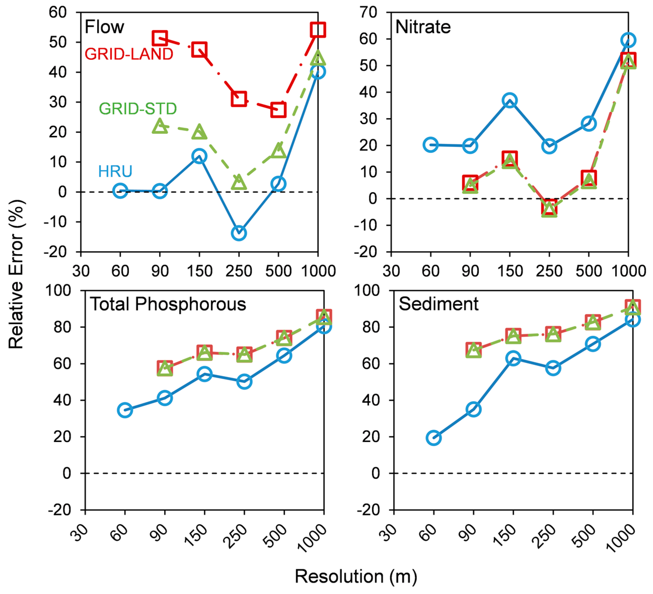
Models’ results were also evaluated in terms of relative error compared to the baseline 30-m HRU model for both flow and water quality. Relative error, average annual discharge and average flow rate shown in Figure 4 and Table 6 indicate that the models follow a similar trend, but that the magnitude of the relative error differs. For the HRU approach, the differences in flow range from <1% to 38.2% and remain under 1% relative error until 90 m. The two GRID approaches follow similar trends with a decrease in relative error from 90- to 250-m spatial resolution, followed by a marked increase in error from 500- to 1000-m resolution. Maximum relative error occurred at 1000 m for all models and a minimum at 90 for HRU, 500 for GRID-LAND and 250 m GRID-STD models, respectively. These differences indicate that discretization and routing do not have a uniform effect on model output, but are both contributing to error. It is likely that decreased flows in the GRID models is due in part to the landscape routing approach moving water from grid to grid, rather than directly to the channel as with standard routing. This allows more opportunity for water to be used in evapotranspiration, infiltration and otherwise be diverted from becoming channelized flow.
Differences in predicted water quality were based on their primary hydrologic transport mechanism. Nitrate relative error trends were similar to flow error given the close link between its mobilization in surface and subsurface flow. Higher nitrate relative error for the HRU models (18% to 29% for HRU, −1% to 13% for GRID-LAND, −3% to 12% GRID-STD) is likely tied to the differences in subsurface flow. In particular, on average, GRID models tended to predict higher nitrate loads relative to the HRU models (22 kg/ha/year HRU, 26 kg/ha/year GRID). Given that (1) soil water content controls nitrogen mineralization within the SWAT model and (2) subsurface water transport and processes were higher for the GRID models (e.g., higher tile flow of 6 mm/year GRID-LAND and 9 mm/year GRID-STD), relatively higher predicted nitrate export of the GRID models is expected. For all models, total phosphorous and sediment slowly increased in relative error with coarsening resolution, where the results of GRID models had a higher relative error (maximum relative error of 65% HRU, 74% GRID for total phosphorous; 72% HRU, 83% GRID for sediment). Phosphorous and sediment transport are more closely linked to transport via surface runoff; thus, the lower runoff of the GRID models (203 mm/year HRU, 184 mm/year GRID) is expected to drive these quantities down compared to the HRU models and increase relative error. The nearly identical relative error between the two GRID approaches for water quality variables is due to a lack of modified nutrient and sediment algorithms to complement the grid-based spatial discretization, which is a known limitation of the current landscape routing approach [20,31]. Furthermore, water quality variables were evaluated at the landscape phase of the simulation, rather than the quantity transported to the watershed outlet, diminishing the effects of the transport mechanism between the GRID approaches.
3.4. Spatial Considerations
Defining an appropriate resolution for simulation is a function of both terrain complexity and topographic attributes [62] for a particular modeled area. These characteristics are related to the input elevation, soils and land use data. As noted previously, other SWAT researchers have found resolution to have little effect on flow [39,40,41,60] or decrease with increasing spatial resolution [36,37] and have suggested a range of appropriate resolutions for HRU-based simulations. The curve number methodology was commonly referred to as a limiting factor in studies where no effect was found on flow (because it is unaffected by slope or the area simulated [40,63]), which is particularly critical for aggregation of DEM data products. Other approaches where slope is explicitly considered, such as TOPMODEL, have found greater flow with coarser spatial resolution [61]. Reducing the resolution of DEMs reduces mean slope and increases slope lengths [37,40,62] and can significantly affect topographic indices [61,64]. From Table 7, slope also decreased with reduced resolution.
The LS (Slope Length and Steepness) factor used in Universal Soil Loss Equation calculations, and to a lesser extent, the curve number also decreased with reduced spatial resolution (Table 7). These values directly relate to the movement and transport of nutrients and sediment, so reduced values contribute to the lower quantities of sediment and nutrients predicted by these models. Accordingly, even when minimal effects on flow occur, resolution still significantly affects water quality predictions [39,40,41,65]. While the recommended coarsest resolution ranges between 100 and 500 m [37,38,39,42,60], results of this analysis are restricted by the inability to simulate SWATgrid at higher resolutions and the choice of relatively coarse STATGO soils data. Although the results suggest 100 m may be appropriate for Cedar Creek and similar Midwestern watersheds, more research is needed.
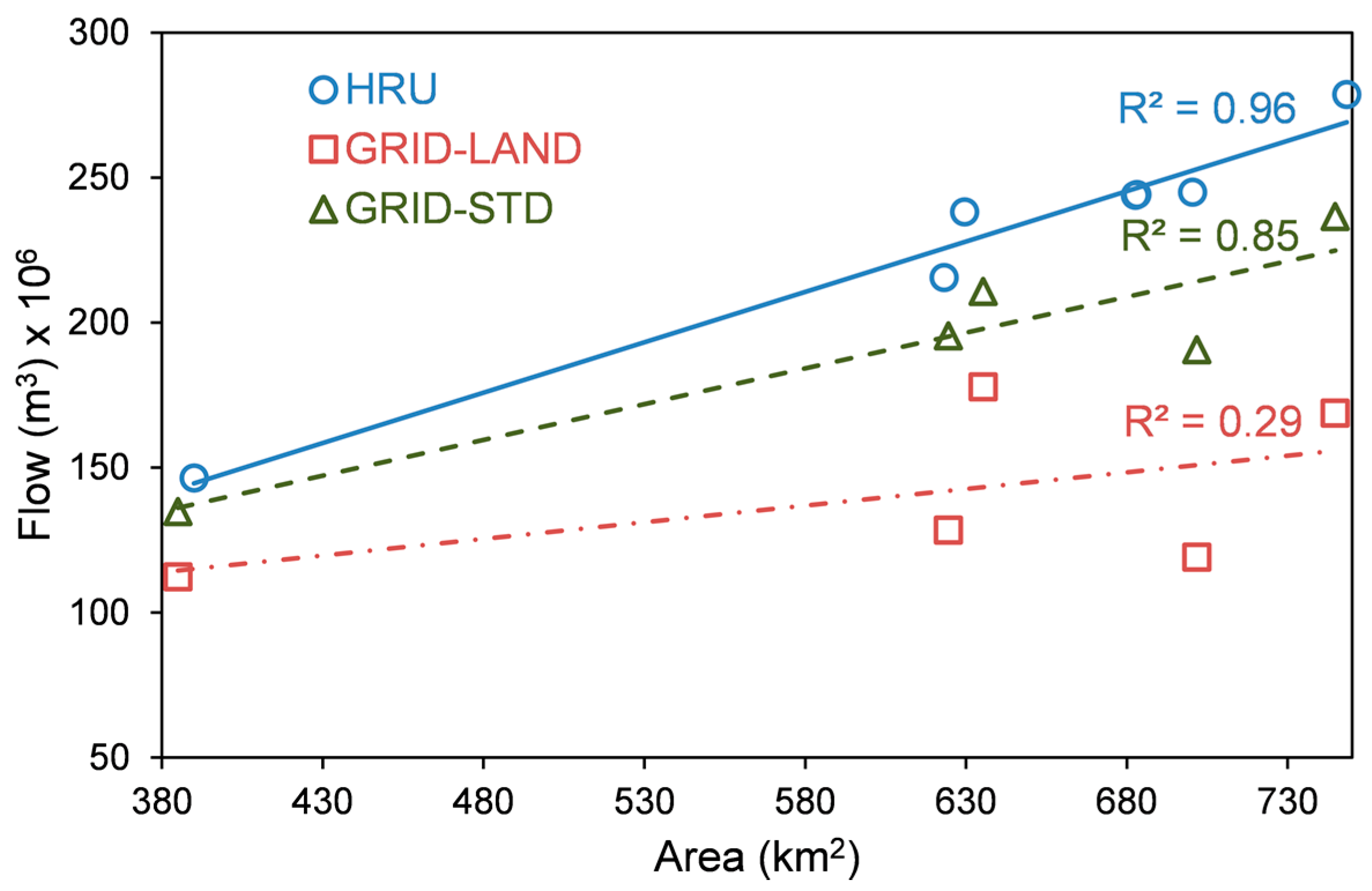
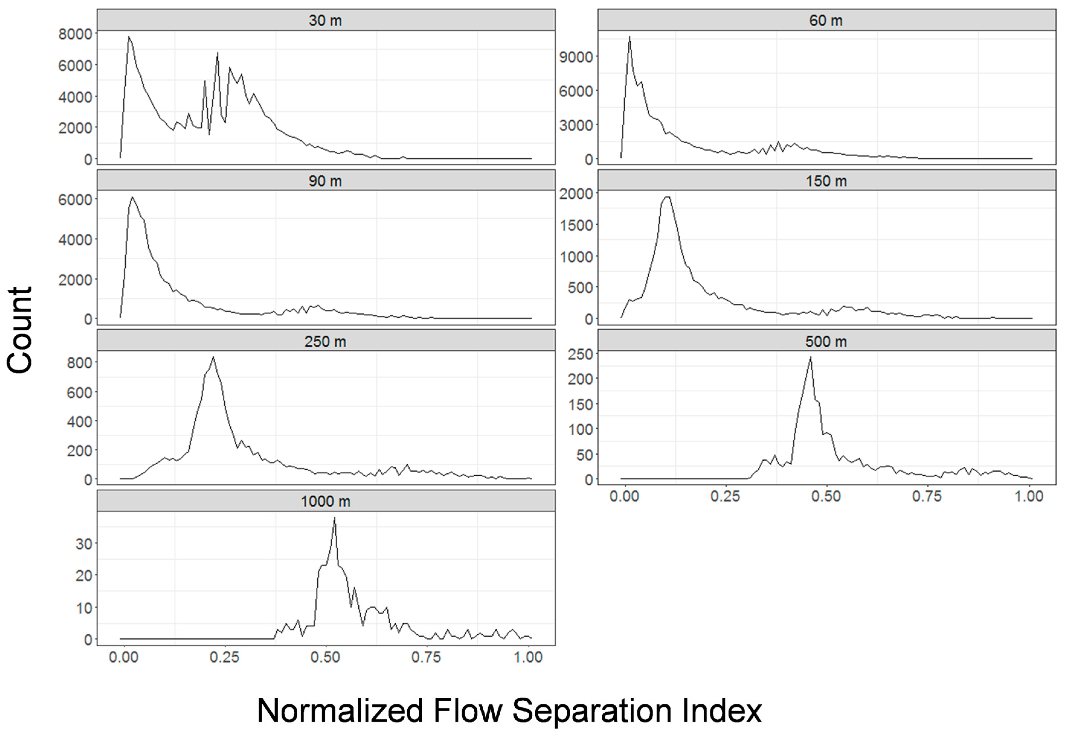
Changes in total watershed area between modeled resolutions is expected to contribute to differences in predictions, where increasing area should lead to increasing flow and nutrient loads. While lower flow was observed on a unit basis for the GRID models (Figure 3 and Figure 4), the relationship between flow and total watershed area was examined for all resolutions of each model type (Figure 5). Although the HRU and GRID-STD approaches follow an expected monotonic relationship of increasing flow with increasing area, for the GRID-LAND approach, this relationship is less pronounced. The key difference between approaches is the use of the flow separation index. Frequency plots of the flow separation index by resolution (Figure 6) show the shift from lower values to high values as resolution is reduced. Given that there are fewer pixels to generate flow at coarser resolution, the flow separation index increases in order to generate more channelized flow. Thus, the GRID-LAND approach relies on both watershed area and the magnitude and distribution of the flow separation index. While previous research has found this index to be highly sensitive to resolution [61] and difficult to validate [29], these results suggest that the GRID-LAND approach responds appropriately by increasing the amount of water that is channelized to account for the smaller number of available grid cells.
The final comparison between models considers the spatial characteristics of simulated output. The primary advantage of SWATgrid, relative to the HRU-based approach, is the ability to simulate and interpret results in a spatially-explicit manner. Results are considered qualitatively, given that models were not individually calibrated. Output for the three model types is shown Figure 7 for surface runoff (SURQ), lateral flow (LATQ) and groundwater flow (GWQ). Results are presented at the scale of model routing, which is the subbasin level for HRU models and the grid cell for GRID models. Much more spatial detail is observable in the GRID models. Surface runoff is related to soil type, where soils with higher infiltration rates (A and B type soils) show lower runoff. The steeper areas in the watershed around channels show greater runoff than flat areas. Banding seen in the northern regions of the maps is due to precipitation gauge distribution. Unlike surface flow, lateral flow is mostly higher in areas of high infiltration and is lower in very flat channelized regions. Groundwater flow is similarly higher in regions of higher infiltration and is much lower in agricultural areas due to the prevalence of tile drainage.
Observed networked flow patterns for the GRID-LAND model are not present in the GRID-STD where landscape routing is removed, as there is no connection of flow components between grid cells. Very high values were observed for some cells of the GRID models, which are the aggregation of landscape flow from several cells. This seems to have occurred in a relatively small fraction of the total cells and had previously been observed and discussed by Rathjens et al. [29]. Overall, the results demonstrate that not only does landscape position matter in simulation, but the spatial distribution of land use and soils is also important.
While the SWATgrid model provides capability to perform simulations in a more spatially-meaningful way, several challenges to broader use remain. In particular, as current computational requirements effectively impede calibration and scenario analysis, applications should focus on spatial analysis for small watersheds (<500 km2), where only a few model runs are necessary and high resolution data can be used as needed. Implementation should reflect modeling needs with the understanding of the advantages and limitations afforded by the SWATgrid approach.
3.5. Calibration Effects
Computational restrictions for the SWATgrid model necessitate transferring calibrated parameters from a standard HRU-based model [33]. Each HRU model developed at 30, 60, 90, 150, 250, 500 and 1000 m was calibrated independently for 5000 total simulations as previously described. The values of the objective function (NSE) were within 5% of each other from 30 to 150 m and then declined thereafter. As the model was calibrated to flow at the outlet, delineated watershed area had a large role in determining the optimized NSE value due to the principles previously examined in the preceding sections.
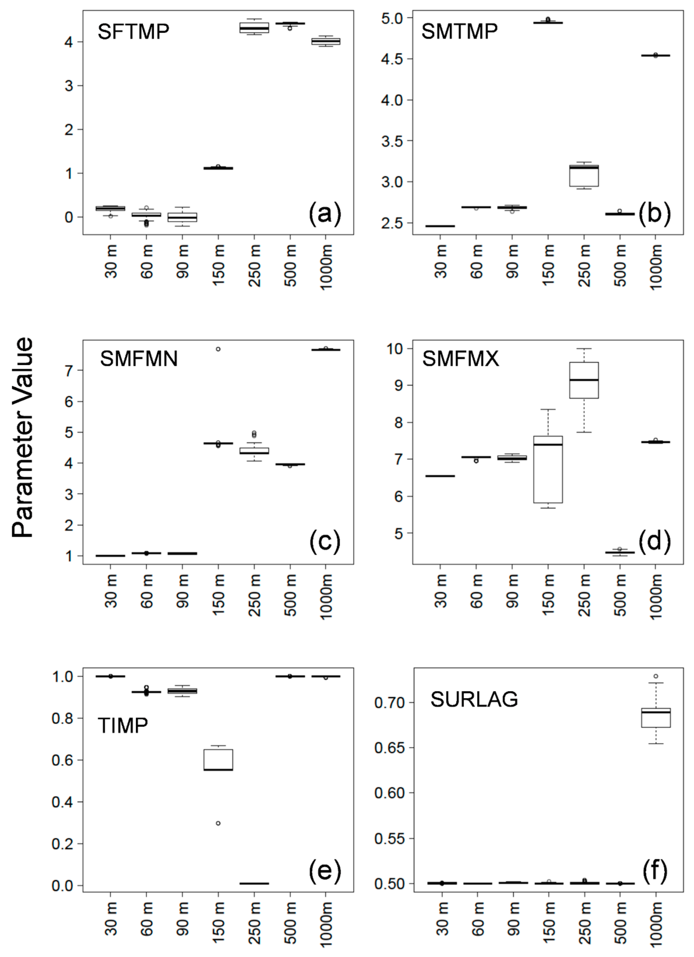
Individual parameter ranges from calibration simulations are shown in Figure 8. For all six calibrated parameters, values tended to be similar in the 30 to 90 m range. This suggests, specific to this model and study area, that parameters may be transferable up to 90 m. However, the scale dependency of parameters must be carefully considered for each model application, as they are often dependent on how landscape representation is aggregated [34]. Previous research has similarly identified a spatial input range of up to 100 m as suitable for watershed modeling [37,60,61,66], although it is empirically based. While response varied by parameter, trends emerged in accordance with expected watershed response. For snow-related parameters for resolutions coarser than 90 m, values trended toward less snow and more water available. For these regions, there is less area to generate flow, with the exception of the 250-m model. Accordingly, the 250-m model shows an opposite trend towards creating and preserving snow, thus lowering flow at the outlet.
While only six parameters were calibrated in this study, the problem of equifinality does not necessarily support inclusion of additional parameters; however, it is similarly difficult to exclude parameters to explicitly minimize equifinality. Therefore, it is important to select appropriate sets of parameter values for calibration that are directly related to the simulated variable being calibrated and that are identified via sensitivity analysis. Understanding how these parameters function in the context of the model framework, as well as their interactions is fundamental to performing a sound calibration.
4. Conclusions
Current SWAT applications utilizing the standard HRU-based approach are limited by the absence of a spatially-explicit landscape position for HRUs. SWATgrid, a gridded approach that utilizes a modified routing algorithm to allow interaction between grid cells, was developed to overcome this limitation. However, SWATgrid remains largely untested with limited understanding of the effects of user-defined input data resolution on simulation results. Further, computational overhead introduced by SWATgrid restricts direct calibration, instead relying on parameter transfer from HRU-based models. To better capture and understand SWATgrid simulations, three objectives were considered: (1) identifying an appropriate resolution for SWATgrid simulations; (2) comparing SWATgrid to commonly-used HRU-based SWAT models; and (3) evaluating the effect of input resolution on model calibration.
Several SWAT models were tested over a range of resolutions with HRU-based, as well as GRID-based approaches, with and without a modified routing technique. Corresponding to each objective, it was found that: (1) flow and water quality simulated outputs tended to decrease with reduced resolution; (2) the SWATgrid approach underpredicted flows and some nutrients; underprediction was greater when using modified routing; and (3) calibrated parameter ranges showed some stability below 90 m. Another key finding was a simulation limit for the GRID approach as a function of both watershed area and grid cell size, which for the watershed tested was 90 m. Differences between HRU-based and GRID models was due to differences in subsurface flows and increased opportunity for loss of water to hydrologic landscape processes in the GRID-LAND approach. Further, the different routing techniques employed by the models likely necessitate separate calibrations, rather than parameter transfer from HRU-based to GRID models, although the transfer may serve as an initial estimate.
Overall, these findings underscore the need for future testing and possible improvements to the SWATgrid approach. However, it is important to recognize that based on the design of this study, the output of the SWATgrid-based models is not necessarily incorrect, but rather different from HRU-based simulations, which were directly calibrated at the 30-m level. In its current state, SWATgrid is most useful in simulating relatively small watersheds (<500 km2) where it is beneficial to capture spatial detail and interaction. As SWATgrid models at 30 and 60 m were not simulated, it is difficult to explicitly define an appropriate scale, although 90 m may be appropriate for watersheds similar to Cedar Creek. Future efforts should focus on a more in-depth analysis of the drivers and causes of simulation differences between SWAT modeling approaches at other locations, improving the calculation and use of the flow separation index, testing the model at higher resolution, using higher resolution soils data and working to improve the computational efficiency of the SWATgrid model. A hybrid approach that utilizes HRU-based SWAT to identify critical subbasins and subsequently modeling these subbasins with the GRID approach may offer an opportunity to synergistically capitalize on the strengths while minimizing the weaknesses of both approaches. Although the choice of model structure and resolution inherently remains a function of the intended application, results from this study can provide guidelines to identify an appropriate approach for future SWATgrid applications in similar regions.
Acknowledgments
We thank Vamsi Krishna Vema, Ph.D. student, Indian Institute of Technology Madras, who provided helpful discussion and insight during the initial development of this research. We additionally thank the anonymous reviewers whose expertise and comments aided in improving the clarity and content of the manuscript.
Author Contributions
Garett Pignotti, Hendrik Rathjens and Raj Cibin conceived of the experiments. Garett Pignotti designed, performed and analyzed the experiments. Raj Cibin developed and guided the model calibration, while Hendrik Rathjens developed and guided the use of SWATgrid during the experiments. Indrajeet Chaubey and Melba Crawford supervised the research as part of Garett Pignotti’s Ph.D. dissertation. Garett Pignotti wrote the paper, and all authors contributed to manuscript revision.
Conflicts of Interest
The authors declare no conflicts of interest.
References
- Karr, J.R.; Schlosser, I.J. Water resources and the land-water interface. Science 1978, 201, 229–234. [Google Scholar] [CrossRef] [PubMed]
- Carpenter, S.R.; Caraco, N.F.; Correll, D.L.; Howarth, R.W.; Sharpley, A.N.; Smith, V.H. Nonpoint pollution of surface waters with phosphorus and nitrogen. Ecol. Appl. 1998, 8, 559–568. [Google Scholar] [CrossRef]
- David, M.B.; Gentry, L.E. Anthropogenic inputs of nitrogen and phosphorus and riverine export for Illinois, USA. J. Environ. Qual. 2000, 29, 494–508. [Google Scholar] [CrossRef]
- Galloway, J.N.; Townsend, A.R.; Erisman, J.W.; Bekunda, M.; Cai, Z.; Freney, J.R.; Martinelli, L.A.; Seitzinger, S.P.; Sutton, M.A. Transformation of the nitrogen cycle: Recent trends, questions, and potential solutions. Science 2008, 320, 889–892. [Google Scholar] [CrossRef] [PubMed]
- Syvitski, J.P.M.; Vörösmarty, C.J.; Kettner, A.J.; Green, P. Impact of humans on the flux of terrestrial sediment to the global coastal ocean. Science 2005, 308, 376–380. [Google Scholar] [CrossRef] [PubMed]
- Pereira, W.; Hostettler, F. Nonpoint source contamination of the Mississippi River and its tributaries by herbicides. Environ. Sci. Technol. 1993, 27, 1542–1552. [Google Scholar] [CrossRef]
- Novotny, V. Water Quality: Diffuse Pollution and Watershed Management; John Wiley & Sons: New York, NY, USA, 2003. [Google Scholar]
- US Environmental Protection Agency National Water Quality Inventory. 2002 Report. Cycle Sect. 305 Clean Water Act; US Environmental Protection Agency National Water Quality Inventory: Washington, DC, USA, 2002.
- Van Griensven, A.; Meixner, T. Methods to quantify and identify the sources of uncertainty for river basin water quality models. Water Sci. Technol. 2006, 53, 51–59. [Google Scholar] [CrossRef] [PubMed]
- Song, X.; Zhang, J.; Zhan, C.; Xuan, Y.; Ye, M.; Xu, C. Global sensitivity analysis in hydrological modeling: Review of concepts, methods, theoretical framework, and applications. J. Hydrol. 2015, 523, 739–757. [Google Scholar] [CrossRef]
- Uusitalo, L.; Lehikoinen, A.; Helle, I.; Myrberg, K. An overview of methods to evaluate uncertainty of deterministic models in decision support. Environ. Model. Softw. 2015, 63, 24–31. [Google Scholar] [CrossRef]
- Krysanova, V.; Arnold, J.G. Advances in ecohydrological modelling with SWAT—A review. Hydrol. Sci. J. 2008, 53, 939–947. [Google Scholar] [CrossRef]
- Borah, D.K.; Bera, M. Watershed-scale hydrologic and nonpoint-source pollution models: Review of mathematical bases. Trans. ASAE 2003, 46, 1553–1566. [Google Scholar] [CrossRef]
- Daniel, E.B.; Camp, J.V.; LeBoeuf, E.J.; Penrod, J.R.; Dobbins, J.P.; Abkowitz, M.D. Watershed modeling and its applications: A state-of-the-art review. Open Hydrol. J. 2011, 5, 26–50. [Google Scholar] [CrossRef]
- Wellen, C.; Kamran-Disfani, A.-R.; Arhonditsis, G.B. Evaluation of the current state of distributed nutrient watershed-water quality modeling. Environ. Sci. Technol. 2015, 49, 3278–3290. [Google Scholar] [CrossRef] [PubMed]
- Blöschl, G.; Sivapalan, M. Scale issues in hydrological modelling: A review. Hydrol. Process. 1995, 9, 251–290. [Google Scholar] [CrossRef]
- Kavetski, D.; Fenicia, F.; Clark, M.P. Impact of temporal data resolution on parameter inference and model identification in conceptual hydrological modeling: Insights from an experimental catchment. Water Resour. Res. 2011, 47, 1–25. [Google Scholar] [CrossRef]
- Perrin, C.; Michel, C.; Andréassian, V. Does a large number of parameters enhance model performance? Comparative assessment of common catchment model structures on 429 catchments. J. Hydrol. 2001, 242, 275–301. [Google Scholar] [CrossRef]
- Das, T.; Bardossy, A.; Zehe, E.; He, Y. Comparison of conceptual model performance using different representations of spatial variability. J. Hydrol. 2008, 356, 106–118. [Google Scholar] [CrossRef]
- Arnold, J.G.; Allen, P.M.; Volk, M.; Williams, J.R.; Bosch, D.D. Assessment of different representations of spatial variability on SWAT model performance. Trans. Am. Soc. Agric. Biol. Eng. 2010, 53, 1433–1443. [Google Scholar]
- Caldwell, P.V.; Kennen, J.G.; Sun, G.; Kiang, J.E.; Butcher, J.B.; Eddy, M.C.; Hay, L.E.; LaFontaine, J.H.; Hain, E.F.; Nelson, S.A.C.; et al. A comparison of hydrologic models for ecological flows and water availability. Ecohydrology 2015, 8, 1525–1546. [Google Scholar] [CrossRef]
- Arnold, J.G.; Srinivasan, R.; Muttiah, R.S.; Williams, J.R. Large area hydrologic modeling and assessment part 1: Model development. J. Am. Water Resour. Assoc. 1998, 34, 73–89. [Google Scholar] [CrossRef]
- Gassman, P.W.; Reyes, M.R.; Green, C.H.; Arnold, J.G. The soil and water assessment tool: Historical development, applications, and future research directions. Trans. ASABE 2007, 50, 1211–1250. [Google Scholar] [CrossRef]
- Douglas-Mankin, K.R.; Srinivasan, R.; Arnold, J.G. Soil and Water Assessment Tool (SWAT) model: Current developments and applications. Trans. ASABE 2010, 53, 1423–1431. [Google Scholar] [CrossRef]
- Manguerra, H.; Engel, B. Hydrologic parameterization of watersheds for runoff prediction using SWAT. J. Am. Water Resour. Assoc. 1998, 34, 1149–1162. [Google Scholar] [CrossRef]
- White, M.J.; Storm, D.E.; Busteed, P.R.; Stoodley, S.H.; Phillips, S.J. Evaluating nonpoint source critical source area contributions at the watershed scale. J. Environ. Qual. 2009, 38, 1654–1663. [Google Scholar] [CrossRef] [PubMed]
- Bosch, D.D.; Arnold, J.G.; Volk, M.; Allen, P.M. Simulation of a low-gradient coastal plain watershed using the swat landscape model. Trans. ASABE 2010, 53, 1445–1456. [Google Scholar] [CrossRef]
- Bonumá, N.B.; Rossi, C.G.; Arnold, J.G.; Reichert, J.M.; Minella, J.P.; Allen, P.M.; Volk, M. Simulating landscape sediment transport capacity by using a modified SWAT model. J. Environ. Qual. 2014, 43, 55. [Google Scholar] [CrossRef] [PubMed]
- Rathjens, H.; Oppelt, N.; Bosch, D.D.; Arnold, J.G.; Volk, M. Development of a grid-based version of the SWAT landscape model. Hydrol. Process. 2014. [Google Scholar] [CrossRef]
- Rathjens, H.; Oppelt, N. SWATgrid: An interface for setting up SWAT in a grid-based discretization scheme. Comput. Geosci. 2012, 45, 161–167. [Google Scholar] [CrossRef]
- Volk, M.; Arnold, J.G.; Bosch, D.D.; Allen, P.M.; Green, C.H. Watershed Configuration and Simulation of Landscape Processes with the SWAT Model. MODSIM 2007 Int. Congr. Model. Simul. 2007, 2383–2389. Available online: https://www.mssanz.org.au/MODSIM07/papers/43_s47/Watersheds47_Volk_.pdf (accessed on 3 January 2017).
- Duku, C.; Rathjens, H.; Zwart, S.J.; Hein, L. Towards ecosystem accounting: A comprehensive approach to modelling multiple hydrological ecosystem services. Hydrol. Earth Syst. Sci. 2015, 19, 4377–4396. [Google Scholar] [CrossRef]
- Rathjens, H.; Oppelt, N. SWAT model calibration of a grid-based setup. Adv. Geosci. 2012, 32, 55–61. [Google Scholar] [CrossRef]
- Feyen, L.; Feyen, J.; Refsgaard, J.C. Effect of grid size on effective parameters and model performance of the MIKE-SHE code. Hydrol. Process 2002, 16, 355–372. [Google Scholar]
- Dixon, B.; Earls, J. Resample or not? Effects of resolution of DEMs in watershed modeling. Hydrol. Process 2009, 23, 1714–1724. [Google Scholar] [CrossRef]
- Cho, S.-M.; Lee, M. Sensitivity considerations when modeling hydrologic processes with Digital Elevation Model. Am. Water Resour. Assoc. 2001, 37, 931–934. [Google Scholar] [CrossRef]
- Chaubey, I.; Cotter, A.S.; Costello, T.A.; Soerens, T.S. Effect of DEM data resolution on SWAT output uncertainty. Hydrol. Process 2005, 628, 621–628. [Google Scholar] [CrossRef]
- Ghaffari, G. The impact of DEM resolution on runoff and sediment modelling results. Res. J. Environ. Sci. 2011, 5, 691–702. [Google Scholar] [CrossRef]
- Chaplot, V. Impact of DEM mesh size and soil map scale on SWAT runoff, sediment, and NO3–N loads predictions. J. Hydrol. 2005, 312, 207–222. [Google Scholar] [CrossRef]
- Lin, S.; Jing, C.; Chaplot, V.; Yu, X.; Zhang, Z.; Moore, N.; Wu, J. Effect of DEM resolution on SWAT outputs of runoff, sediment and nutrients. Hydrol. Earth Syst. Sci. Discuss. 2010, 7, 4411–4435. [Google Scholar] [CrossRef]
- Shen, Z.Y.; Chen, L.; Liao, Q.; Liu, R.M.; Huang, Q. A comprehensive study of the effect of GIS data on hydrology and non-point source pollution modeling. Agric. Water Manag. 2013, 118, 93–102. [Google Scholar] [CrossRef]
- Zhang, P.; Liu, R.; Bao, Y.; Wang, J.; Yu, W.; Shen, Z. Uncertainty of SWAT model at different DEM resolutions in a large mountainous watershed. Water Res. 2014, 53, 132–144. [Google Scholar] [CrossRef] [PubMed]
- Xie, H.; Chen, L.; Shen, Z. Assessment of agricultural best management practices using models: Current issues and future perspectives. Water 2015, 7, 1088–1108. [Google Scholar] [CrossRef]
- Heathman, G.C.; Larose, M.; Ascough, J.C. Soil and Water Assessment Tool evaluation of soil and land use geographic information system data sets on simulated stream flow. J. Soil Water Conserv. 2009, 64, 17–32. [Google Scholar] [CrossRef]
- Han, E.; Merwade, V.; Heathman, G.C. Application of data assimilation with the Root Zone Water Quality Model for soil moisture profile estimation in the upper Cedar Creek, Indiana. Hydrol. Process 2012, 26, 1707–1719. [Google Scholar] [CrossRef]
- Heathman, G.C.; Cosh, M.H.; Han, E.; Jackson, T.J.; McKee, L.; McAfee, S. Field scale spatiotemporal analysis of surface soil moisture for evaluating point-scale in situ networks. Geoderma 2012, 170, 195–205. [Google Scholar] [CrossRef]
- Neitsch, S.L.; Arnold, J.G.; Kiniry, J.R.; Williams, J.R. Soil & Water Assessment Tool—Theoretical Documentation Version 2009. Texas Water Resour. Inst. 2011. Available online: swat.tamu.edu/media/99192/swat2009-theory.pdf (accessed on 3 January 2017).
- Garbrecht, J.; Martz, L. Grid size dependency of parameters extracted from digital elevation models. Comput. Geosci. 1994, 20, 85–87. [Google Scholar] [CrossRef]
- Her, Y.; Chaubey, I.; Frankenberger, J.; Smith, D. Effect of conservation practices implemented by USDA programs at field and watershed scales. J. Soil Water Conserv. 2016, 71, 249–266. [Google Scholar] [CrossRef]
- Jaynes, D.; James, D. The Extent of Farm Drainage in the United States. US Dep. Agric. 2007. Available online: https://www.ars.usda.gov/ARSUserFiles/50301500/theextentoffarmdrainageintheunitedstates.pdf (accessed on 3 January 2017).
- Kalcic, M.M.; Frankenberger, J.; Chaubey, I. Spatial optimization of six conservation practices using SWAT in tile-drained agricultural watersheds. J. Am. Water Resour. Assoc. 2015, 51, 956–972. [Google Scholar] [CrossRef]
- Arnold, J.G.; Allen, P.M.; Muttiah, R.; Bernhardt, G. Automated base flow separation and recession analysis techniques. Ground Water 1995, 33, 1010–1018. [Google Scholar] [CrossRef]
- Arnold, J.G.; Allen, P.M. Automated methods for estimating baseflow and ground water recharge from streamflow records. J. Am. Water Resour. Assoc. 1999, 35, 411–424. [Google Scholar] [CrossRef]
- Cibin, R.; Trybula, E.; Chaubey, I.; Brouder, S.M.; Volenec, J.J. Watershed-scale impacts of bioenergy crops on hydrology and water quality using improved SWAT model. GCB Bioenergy 2016, 8, 837–848. [Google Scholar] [CrossRef]
- Vrugt, J.A.; Robinson, B.A. Improved evolutionary optimization from genetically adaptive multimethod search. Proc. Natl. Acad. Sci. USA 2007, 104, 708–711. [Google Scholar] [CrossRef] [PubMed]
- Nash, J.E.; Sutcliffe, J.V. River flow forecasting through conceptual models: Part I-A discussion of principles. J. Hydrol. 1970, 10, 282–290. [Google Scholar] [CrossRef]
- Rees, W.G. The accuracy of Digital Elevation Models interpolated to higher resolutions. Int. J. Remote Sens. 2000, 21, 7–20. [Google Scholar] [CrossRef]
- Tan, M.L.; Ficklin, D.L.; Dixon, B.; Ibrahim, A.L.; Yusop, Z.; Chaplot, V. Impacts of DEM resolution, source, and resampling technique on SWAT-simulated streamflow. Appl. Geogr. 2015, 63, 357–368. [Google Scholar] [CrossRef]
- Beven, K. A manifesto for the equifinality thesis. J. Hydrol. 2006, 320, 18–36. [Google Scholar] [CrossRef]
- Cotter, A.S.; Chaubey, I.; Costello, T.A.; Soerens, T.S.; Nelson, M.A. Water quality model output uncertainty as affected by spatial resolution of input data. J. Am. Water Resour. Assoc. 2004, 39, 977–986. [Google Scholar] [CrossRef]
- Brasington, J.; Richards, K. Interactions between model predictions, parameters and DTM scales for TOPMODEL. Comput. Geosci. 1998, 24, 299–314. [Google Scholar] [CrossRef]
- Wu, S.; Li, J.; Huang, G.H. A study on DEM-derived primary topographic attributes for hydrologic applications: Sensitivity to elevation data resolution. Appl. Geogr. 2008, 28, 210–223. [Google Scholar] [CrossRef]
- Jha, M.; Gassman, P.W.; Secchi, S.; Gu, R.; Arnold, J. Effect of Watershed Subdivision on SWAT Flow, Sediment, and Nutrient Predictions. J. Am. Water Resour. Assoc. 2004, 40, 811–825. [Google Scholar] [CrossRef]
- Sørensen, R.; Seibert, J. Effects of DEM resolution on the calculation of topographical indices: TWI and its components. J. Hydrol. 2007, 347, 79–89. [Google Scholar] [CrossRef]
- Wu, S.; Li, J.; Huang, G. An evaluation of grid size uncertainty in empirical soil loss modeling with digital elevation models. Environ. Model. Assess. 2005, 10, 33–42. [Google Scholar] [CrossRef]
- Rojas, R.; Velleux, M.; Julien, P.Y.; Johnson, B.E. Grid scale effects on watershed soil erosion models. J. Hydrol. Eng. 2008, 13, 793–802. [Google Scholar] [CrossRef]
Figure 1.
Cedar Creek Watershed characteristics: (a) elevation (National Elevation Data (NED) 30 m) with the stream and precipitation gauging stations shown; (b) soil hydrologic group (State Soil Geographic (STATSGO) 250 m); and (c) land use (reclassified from NASS 2010 Crop Data Layer (CDL) 30 m).
Figure 1.
Cedar Creek Watershed characteristics: (a) elevation (National Elevation Data (NED) 30 m) with the stream and precipitation gauging stations shown; (b) soil hydrologic group (State Soil Geographic (STATSGO) 250 m); and (c) land use (reclassified from NASS 2010 Crop Data Layer (CDL) 30 m).
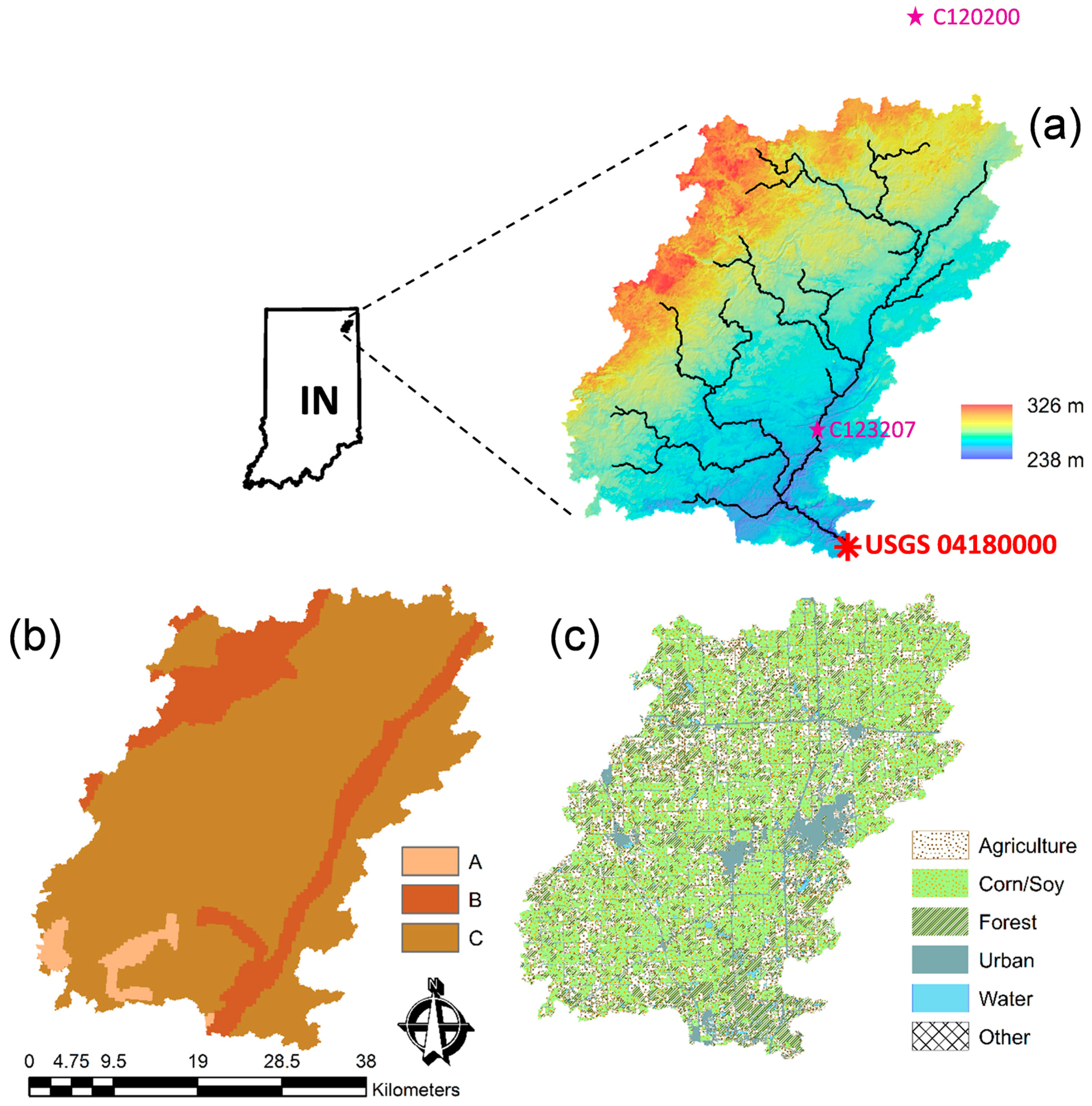
Figure 2.
Comparison of observed and simulated monthly flow at the watershed outlet for the baseline 30-m Cedar Creek HRU model. Calibration period is 1994 to 2003, and the validation is 2004 to 2010.
Figure 2.
Comparison of observed and simulated monthly flow at the watershed outlet for the baseline 30-m Cedar Creek HRU model. Calibration period is 1994 to 2003, and the validation is 2004 to 2010.
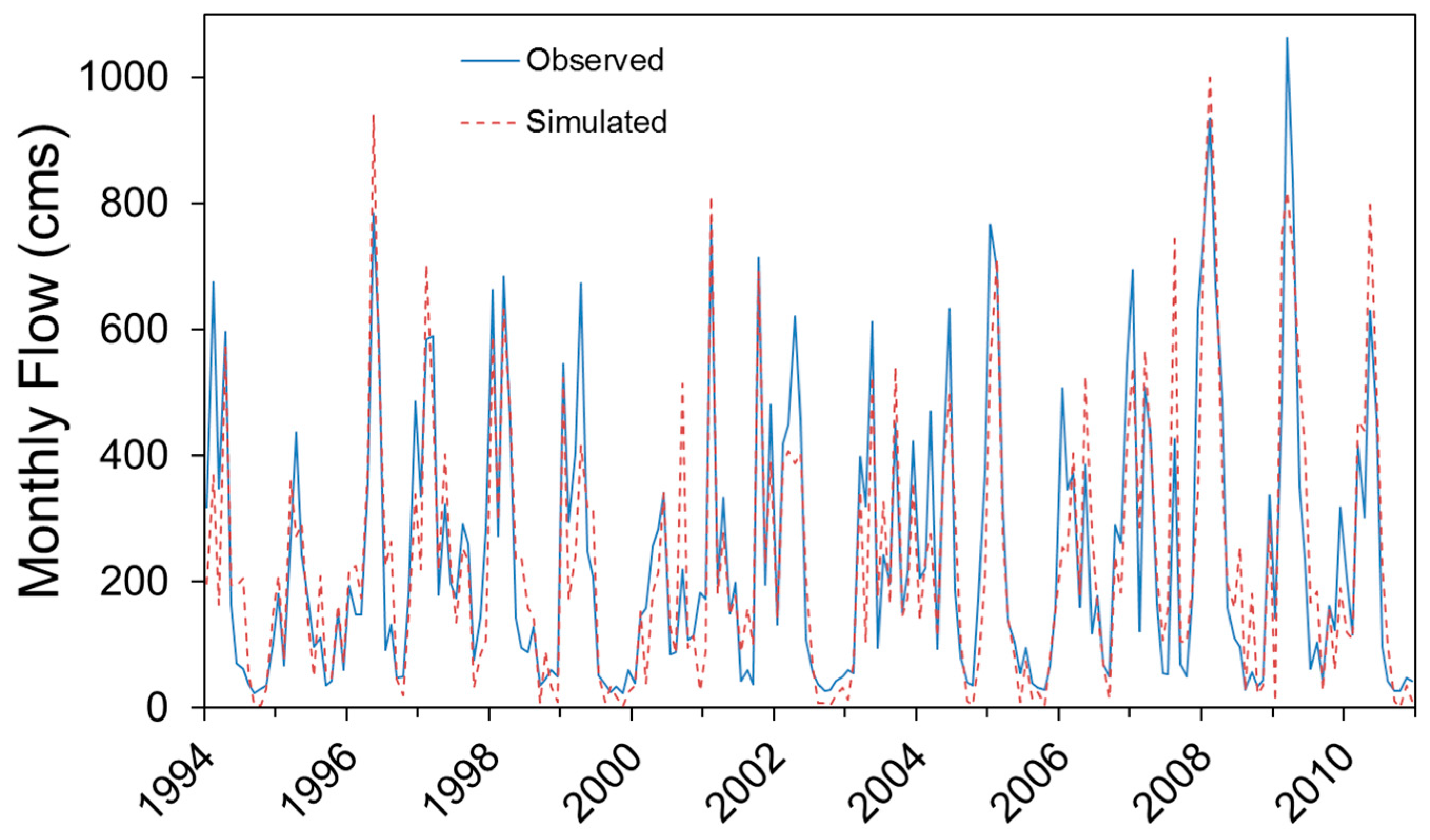
Figure 3.
Hydrologic simulations for 90-m resolution models’ (a) monthly hydrographs and (b) average monthly absolute flow difference relative to the HRU model.
Figure 3.
Hydrologic simulations for 90-m resolution models’ (a) monthly hydrographs and (b) average monthly absolute flow difference relative to the HRU model.
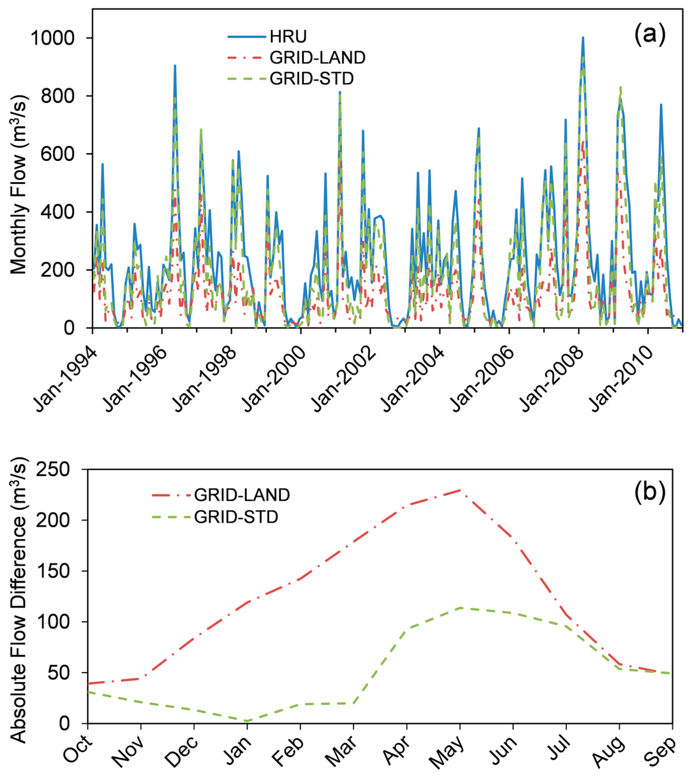
Figure 4.
Average relative model error as compared to the 30-m Cedar Creek HRU model.

Figure 5.
Effect of area on average annual total stream flow for each model approach.

Figure 6.
Frequency plots of normalized flow separation indices by resolution.

Figure 7.
Spatial output for selected annual average surface runoff (SURQ), lateral flow (LATQ) and groundwater flow (GWQ) for all model types at 90-m resolution. Values plotted at the unit of transport (i.e., subbasins and grid cells) at the scale maximize visual contrast. STD, standard.
Figure 7.
Spatial output for selected annual average surface runoff (SURQ), lateral flow (LATQ) and groundwater flow (GWQ) for all model types at 90-m resolution. Values plotted at the unit of transport (i.e., subbasins and grid cells) at the scale maximize visual contrast. STD, standard.
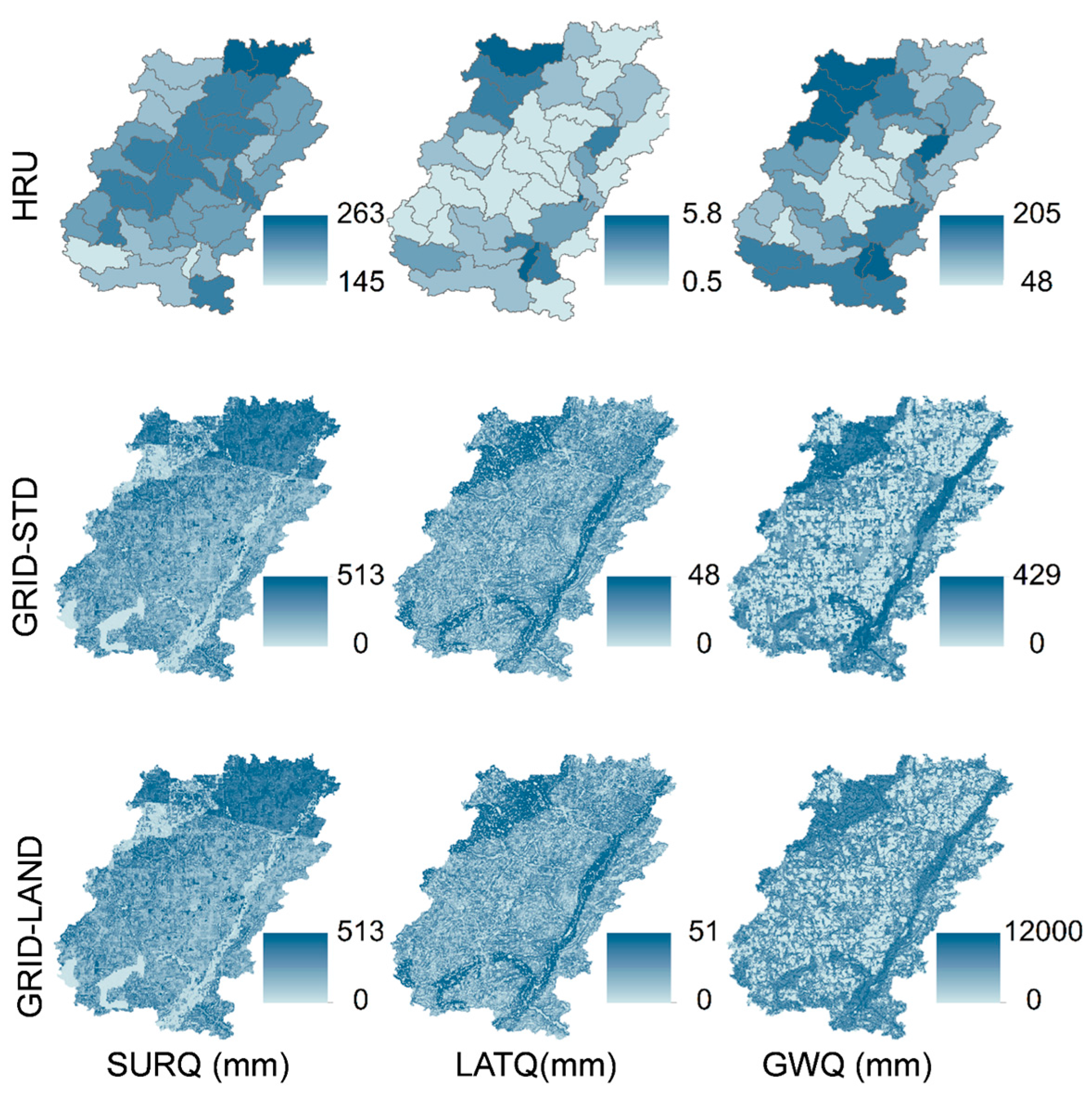
Figure 8.
Calibrated parameter ranges by resolution for: (a) snowfall temperature (SFTMP); (b) snow melt temperature (SMTMP); (c) snow minimum melt factor (SMFMN); (d) snow maximum melt factor (SMFMX); (e) snow pack temperature lag factor (TIMP); and (f) surface runoff lag coefficient (SURLAG).
Figure 8.
Calibrated parameter ranges by resolution for: (a) snowfall temperature (SFTMP); (b) snow melt temperature (SMTMP); (c) snow minimum melt factor (SMFMN); (d) snow maximum melt factor (SMFMX); (e) snow pack temperature lag factor (TIMP); and (f) surface runoff lag coefficient (SURLAG).


Table 1.
Agricultural management implemented in models.
| Management Strategy | ||
|---|---|---|
| Date | Operation | |
| Corn Year | 22 April | N Application 1 |
| 22 April | Atrazine 2 | |
| 6 May | Cultivator | |
| 6 May | Planting | |
| 6 June | N Application 3 | |
| 14 October | Harvesting | |
| 15 October | Killing | |
| Soybean Year | 24 May | Zero Till |
| 24 May | Planting | |
| 7 October | Harvesting | |
| 8 October | Killing | |
| 15 October | P Application 4 | |
| 1 November | Chisel | |
Notes: 1 Anhydrous of 53 kg/ha (N of 43 kg/ha); 2 atrazine of 2.2 kg/ha; 3 urea of 284 kg/ha (N of 131 kg/ha); 4 Diammonium phosphate (DAP) (P2O5) of 123 kg/ha (P of 54 kg/ha).
Table 2.
Tile drainage parameters implemented on rotational corn and soybean land use with poorly- or very poorly-drained soils.
Table 2.
Tile drainage parameters implemented on rotational corn and soybean land use with poorly- or very poorly-drained soils.
| Parameter | Definition | Value |
|---|---|---|
| DDRAIN (mm) | Depth from surface to tile drains | 1000 |
| TDRAIN (h) | Time to drain to field capacity | 24 |
| GDRAIN (h) | Drainage lag time | 48 |
| DEP_IMP (mm) | Depth from surface to impervious layer | 1200 |
| ITDRN (flag) | Drainage routine (1 indicates ‘new’ routine) | 1 |
| RE (mm) | Effective drain radius | 20 |
| SDRAIN (mm) | Distance between tile drains | 20,000 |
| DRAIN_CO (mm/day) | Drainage coefficient | 10 |
| PC (mm/h) | Pump capacity | 0 |
| LATKSATF | Multiplication factor for lateral conductivity | 1.2 |
Table 3.
Calibrated parameters for the 30-m baseline hydrological response unit (HRU) model.
| Parameter | Definition | Units | Range | Default | Calibrated |
|---|---|---|---|---|---|
| SFTMP | snowfall temperature | °C | −5 to 5 | 1 | 0.18 |
| SURLAG | surface runoff lag coefficient | day | 0.5 to 2 | 4 | 0.50 |
| SMTMP | snow melt base temperature | °C | −5 to 5 | 0.5 | 2.46 |
| TIMP | snow pack temperature lag factor | - | 0.01 to 1 | 1 | 1.00 |
| SMFMX | maximum melt factor | mm H2O/°C | 1 to 10 | 4.5 | 6.54 |
| SMFMN | minimum melt factor | mm H2O/°C | 1 to 10 | 4.5 | 1.00 |
Table 4.
Monthly calibration and validation results for flow.
| Metric | Calibration | Validation |
|---|---|---|
| Monthly NSE | 0.80 | 0.80 |
| Observed Mean (m3/s) | 7.48 | 8.67 |
| Simulated Mean (m3/s) | 7.13 | 8.66 |
Table 5.
Model input characteristics based on spatial input resolution.
| Resolution (m) | HRU Watershed Area (km2) | HRU Subbasins | GRID Watershed Area (km2) | GRID Cells | GRID Simulation Time (min) |
|---|---|---|---|---|---|
| 30 | 700.4 | 43 | - | - | - |
| 60 | 682.7 | 41 | - | - | - |
| 90 | 683.1 | 42 | 701.7 | 86,635 | 6456 |
| 150 | 623.1 | 35 | 624.4 | 27,253 | 693 |
| 250 | 748.4 | 45 | 744.8 | 11,916 | 149 |
| 500 | 629.5 | 29 | 635.3 | 2451 | 12 |
| 1000 | 390.0 | 17 | 385.0 | 385 | 1 |
Table 6.
Average annual predictions based on resolution and model type.
| Model | Flow † (m3) | Flow (mm) | Nitrate (Mg) | Nitrate (kg/ha) | Total P (Mg) | Total P (kg/ha) | Sediment (Mg) | Sediment (kg/ha) |
|---|---|---|---|---|---|---|---|---|
| 30 HRU | 245 | 350 | 1910 | 27.3 | 229 | 3.27 | 197,400 | 2820 |
| 60 HRU | 244 | 357 | 1524 | 22.3 | 150 | 2.20 | 159,100 | 2330 |
| 90 HRU | 244 | 357 | 1531 | 22.4 | 135 | 1.97 | 128,200 | 1880 |
| 150 HRU | 216 | 346 | 1204 | 19.3 | 105 | 1.68 | 73,200 | 1170 |
| 250 HRU | 279 | 372 | 1534 | 20.5 | 114 | 1.53 | 83,700 | 1120 |
| 500 HRU | 238 | 378 | 1371 | 21.8 | 82 | 1.30 | 57,600 | 915 |
| 1000 HRU | 146 | 375 | 772 | 19.8 | 45 | 1.15 | 3100 | 796 |
| 90 STD | 191 | 272 | 1817 | 25.9 | 97 | 1.39 | 64,200 | 915 |
| 150 STD | 195 | 313 | 1639 | 26.3 | 78 | 1.24 | 49,000 | 785 |
| 250 STD | 237 | 318 | 1988 | 26.7 | 80 | 1.07 | 46,900 | 630 |
| 500 STD | 211 | 332 | 1784 | 28.1 | 59 | 0.93 | 34,100 | 536 |
| 1000 STD | 135 | 350 | 924 | 24.0 | 33 | 0.86 | 17,900 | 465 |
| 90 LAND | 119 | 170 | 1796 | 25.6 | 97 | 1.39 | 64,200 | 915 |
| 150 LAND | 128 | 206 | 1623 | 26.0 | 78 | 1.25 | 49,000 | 785 |
| 250 LAND | 169 | 227 | 1969 | 26.4 | 80 | 1.08 | 47,000 | 631 |
| 500 LAND | 178 | 280 | 1761 | 27.7 | 59 | 0.94 | 34,100 | 537 |
| 1000 LAND | 112 | 292 | 915 | 23.8 | 33 | 0.86 | 1800 | 467 |
Note: † Millions (1 × 10⁶).
Table 7.
Selected average input characteristics based on resolution and model type.
| Model | Area (km2) | Mean Slope | Mean CN2 | Mean USLE-LS |
|---|---|---|---|---|
| 30 HRU | 700 | 0.278 | 76.7 | 0.432 |
| 60 HRU | 683 | 0.201 | 75.8 | 0.304 |
| 90 HRU | 683 | 0.016 | 75.8 | 0.244 |
| 150 HRU | 623 | 0.012 | 76.4 | 0.183 |
| 250 HRU | 748 | 0.008 | 75.6 | 0.139 |
| 500 HRU | 630 | 0.005 | 76.0 | 0.110 |
| 1000 HRU | 390 | 0.003 | 75.8 | 0.093 |
| 90 GRID | 702 | 0.210 | 73.7 | 0.439 |
| 150 GRID | 624 | 0.017 | 73.5 | 0.317 |
| 250 GRID | 745 | 0.012 | 72.7 | 0.215 |
| 500 GRID | 635 | 0.008 | 72.8 | 0.146 |
| 1000 GRID | 385 | 0.005 | 72.3 | 0.110 |
© 2017 by the authors. Licensee MDPI, Basel, Switzerland. This article is an open access article distributed under the terms and conditions of the Creative Commons Attribution (CC BY) license (http://creativecommons.org/licenses/by/4.0/).
Share and Cite
MDPI and ACS Style
Pignotti, G.; Rathjens, H.; Cibin, R.; Chaubey, I.; Crawford, M. Comparative Analysis of HRU and Grid-Based SWAT Models. Water 2017, 9, 272. https://doi.org/10.3390/w9040272
AMA Style
Pignotti G, Rathjens H, Cibin R, Chaubey I, Crawford M. Comparative Analysis of HRU and Grid-Based SWAT Models. Water. 2017; 9(4):272. https://doi.org/10.3390/w9040272
Chicago/Turabian StylePignotti, Garett, Hendrik Rathjens, Raj Cibin, Indrajeet Chaubey, and Melba Crawford. 2017. "Comparative Analysis of HRU and Grid-Based SWAT Models" Water 9, no. 4: 272. https://doi.org/10.3390/w9040272
Note that from the first issue of 2016, this journal uses article numbers instead of page numbers. See further details here.