
The Impact of Integrated Aquifer Storage and Recovery and Brackish Water Reverse Osmosis (ASRRO) on a Coastal Groundwater System

KWR Watercycle Research Institute, P.O. Box 1072, 3430 BB Nieuwegein, The Netherlands
*
Author to whom correspondence should be addressed.
Water 2017, 9(4), 273; https://doi.org/10.3390/w9040273
Submission received: 31 October 2016
/
Revised: 6 April 2017
/
Accepted: 6 April 2017
/
Published: 12 April 2017
(This article belongs to the Special Issue Water Quality Considerations for Managed Aquifer Recharge Systems)
Abstract
:Aquifer storage and recovery (ASR) of local, freshwater surpluses is a potential solution for freshwater supply in coastal areas, as is brackish water reverse osmosis (BWRO) of relatively shallow groundwater in combination with deeper membrane concentrate disposal. A more sustainable and reliable freshwater supply may be achieved by combining both techniques in one ASRRO system using multiple partially penetrating wells (MPPW). The impact of widespread use of ASRRO on a coastal groundwater system was limited based on regional groundwater modelling but it was shown that ASRRO decreased the average chloride concentration with respect to the autonomous scenario and the use of BWRO. ASRRO was successful in mitigating the local negative impact (saltwater plume formation) caused by the deep disposal of membrane concentrate during BWRO. The positive impacts of ASRRO with respect to BWRO were observed in the aquifer targeted for ASR and brackish water abstraction (Aquifer 1), but foremost in the deeper aquifer targeted for membrane concentrate disposal (Aquifer 2). The formation of a horizontal freshwater barrier was found at the top of both aquifers, reducing saline seepage. The disposal of relatively fresh concentrate in Aquifer 2 led to brackish water outflow towards the sea. The net abstraction in Aquifer 1 enforced saltwater intrusion, especially when BWRO was applied. The conclusion of this study is that ASRRO can provide a sustainable alternative for BWRO.
1. Introduction
Coastal areas are often marked by high freshwater demands and a low freshwater availability. Use of aquifer storage and recovery (ASR; [1,2]) of temporary freshwater surpluses and brackish water reverse osmosis (BWRO; [3]) are potential techniques to improve the freshwater availability in coastal areas. ASR is a cost-effective, readily applicable technique to store large water volumes without the occupation of large surface areas. Nevertheless, the performance of ASR, which is marked by the recovery efficiency (RE: the percentage of freshwater that can be recovered upon storage), can be very limited in coastal areas [4]. The main cause for the reduced RE are the buoyancy effects induced by the difference in density of the brackish or saline native groundwater (high density), and the injected freshwater (low density). This leads to early salinization at the bottom of the ASR well [5,6,7]. On the other hand, BWRO is a proven technology able to continuously desalinate groundwater with a wide range of salinities, while its costs are acceptable for various end users. However, BWRO is accompanied by a saline waste stream (membrane concentrate: ‘MC’). Disposal of this MC often occurs into (deeper) aquifers or local surface waters, which can lead to environmental pollution and/or groundwater salinization.
A more sustainable and reliable freshwater supply can potentially be achieved by combining ASR and RO in one system (‘ASRRO’, Figure 1). In such a set-up, a balance is obtained between freshwater injection (wet periods) and recovery (dry periods) via a combination of ASR and BWRO-treatment. Doing so, the abstraction of brackish groundwater at the base of the ASR target aquifer for BWRO may improve the direct recovery of freshwater by shallower wells [8] and thus the RE of ASR. The deep well intercepting brackish water is called a ‘Freshkeeper’ [9]. The integrated approach of ASRRO may provide a much more robust and sustainable freshwater supply than each of the independent techniques, as more freshwater is recoverable for direct use, such that less water requires (energy-consuming) desalination by RO. Additionally, overexploitation of the groundwater may be counteracted by compensating freshwater production with artificial recharge.
A first ASRRO system was constructed in 2012 and tested as a conventional ASR-system in the first year (2013), while the Freshkeeper well was added in 2014 [10]. Since 2015, the system is operating as a complete ASRRO system. In the first studies, the focus was on the direct recoverability of the injected freshwater [10] and potential clogging of the RO-membrane [11]. However, the impact of ASRRO on the local and regional groundwater system was not evaluated. The aim of this study is therefore to analyse the effects of ASRRO on the groundwater quality in a coastal area, both on a local and a regional scale. The design and operation of ASRRO were derived from a field pilot, situated centrally in the study area [10]. Numerical modelling was performed to assess the water quality development of the Regional groundwater system.
2. Methods
2.1. Study Area
The Westland area in The Netherlands is the country’s largest intensive greenhouse horticultural area and situated within 10 km of the North Sea shoreline (Figure 2). It suffers from a significant mismatch between water demand and availability in the horticultural greenhouse sector, presence of brackish and saline groundwater, current use of BWRO, and saltwater intrusion [12]. The horticultural sector in the area requires irrigation water with an extremely low salinity of <0.5 mmol/L [4]. Surface water and drinking water generally fail to meet this water quality limit. Therefore, rainwater is harvested via the greenhouses’ roofs and partly stored in aboveground basins. A mismatch in precipitation and water demand, however, results in discharge of a significant part of the available rainwater in wet periods [4]. Therefore, BWRO is required in summers as additional fresh irrigation water supply. Greenhouse owners in the area using BWRO abstract the required brackish groundwater from the upper Aquifer 1 (10–50 m BSL) and dispose of MC in the deeper Aquifer 2 (40–120 m BSL).
Because of the presence of confined, unconsolidated sand aquifers in the shallow subsurface (10–50 m BSL), ASR is a viable option to bridge the periods of rainwater availability and demand [4]. However, although the upper aquifer is the least saline target aquifer for ASR available, the predicted RE of ASR is generally <50% in the Westland area [4]. Therefore, attempts are being made to improve the RE of ASR via independently operated multiple partially penetrating wells in a single borehole (MPPW, [13]).
2.2. Numerical Modelling of ASRRO Application
Since ASRRO is still in a piloting phase and observation of all complex interactions is hard in the field, the impact on the groundwater quality in the area was assessed by numerical modelling. A two-stage approach was applied by first modelling two individual ASRRO systems in a horizontal layer model to study their performance and interaction on a local scale (based on the field pilot: Local Model), followed by modelling of the widespread use of ASRRO in the Westland region (Regional Model). In both cases, SEAWAT Version 4 [14] was used. FloPy [15] was used to generate the models’ input and output and to frequently calculate the resulting MC concentration, which provided input to the Source/Sink package in the subsequent stress period.
2.2.1. Modelling Local Impacts (Local Model Based on ASRRO Pilot)
A half-domain (2 × 0.5 km) local model was set up and comprises two ASRRO systems, of which the design and setting was based on the general design, operation, and setting of the first ASRRO field trial [10]. The main model parameters are shown in Table 1 and are based on an extensive ASR pilot in the target sand aquifer in the Westland area, which included calibrated groundwater modelling [10]. The parameterisation was considered representative for the target area. A dispersivity coefficient of 0.1 m was assigned based on the same pilots in the same aquifer [10,13] and a diffusion coefficient of 8.64 × 10⁻⁵ m2/day was assigned based on [10,16]. The grid size varied spatially and was most refined near the wells, i.e., either 5 m (x) × 5 m (y) × 1.5 m (z) at the MPPWs and 5 m × 5 m × 4 m at the membrane concentrate disposal wells (MC disposal well). Western and eastern boundaries were assigned a general head boundary (GHB). The GHB simulated a constant head at a distance of half a cell length (L) from the model boundaries (20 m), using the heads marked in Figure 3 and assuming unchanged horizontal conductivity (Kh). The GHB conductance (CGHB) depended on the boundary cells’ width (W) and thickness (D) perpendicular to the regional flow direction and was calculated using
Concentrations at these boundaries were kept constant and were based on [10]. A hydraulic gradient of −0.008 m/m induced background flow as indicated in Figure 3 and was based on the regional heads (Figure 2). Recharge by precipitation was not considered because the target areas for ASRRO are typically covered with greenhouses clusters (capturing rainfall, which is infiltrated with the ASRRO systems) and infiltration through the thick clay cover is limited.
An autonomous case without wells was for comparison with ASRRO and BWRO cases. Subsequently, two scenarios were evaluated with transient models: one with the ASRRO systems (infiltration of winter surplus equals combined freshwater production from ASR and RO (+MC disposal) in summer), the other with the conventional BWRO systems (no infiltration in winter) to produce the same volume of freshwater solely from BWRO in summer while reinjecting MC. The average winter precipitation surplus available for ASR is around 200 mm/year or 2000 m3/ha of greenhouse [17]. The impact of ASRRO systems was determined for a predefined 27-ha greenhouse area (Figure 3), which simulates 2 ASRRO systems in a half-domain with areas equal to the area connected to the pilot ASRRO system [10]. Accordingly, 54,000 m3/year of freshwater was injected by MPPWs (coded ‘a–d’) in Aquifer 1 in winter and abstracted in the next summer after a 59-days’ storage period. The operational schemes of the BWRO and ASRRO cases are shown in Table 2. Unmixed freshwater for direct use was recovered first during ASRRO. Upon salinization of the recovery wells, the water was directed to the RO to produce freshwater. The MC was injected into Aquifer 2 via the MC disposal wells. An RO efficiency of 50% (maximal achievable efficiency without anti-scalants) was assumed in both scenarios, resulting in an equal production of freshwater and MC. In total, a net volume of 54,000 m3 of freshwater is produced from Aquifer 1 during both ASRRO and BWRO each year. This is ca. 4.4% and 1.6% of the pore water volume present in Aquifer 1 (1,215,000 m3) and Aquifer 2 (3,402,000 m3) in the 27-ha subsection.
2.2.2. Modelling of Regional Impact (Regional Model)
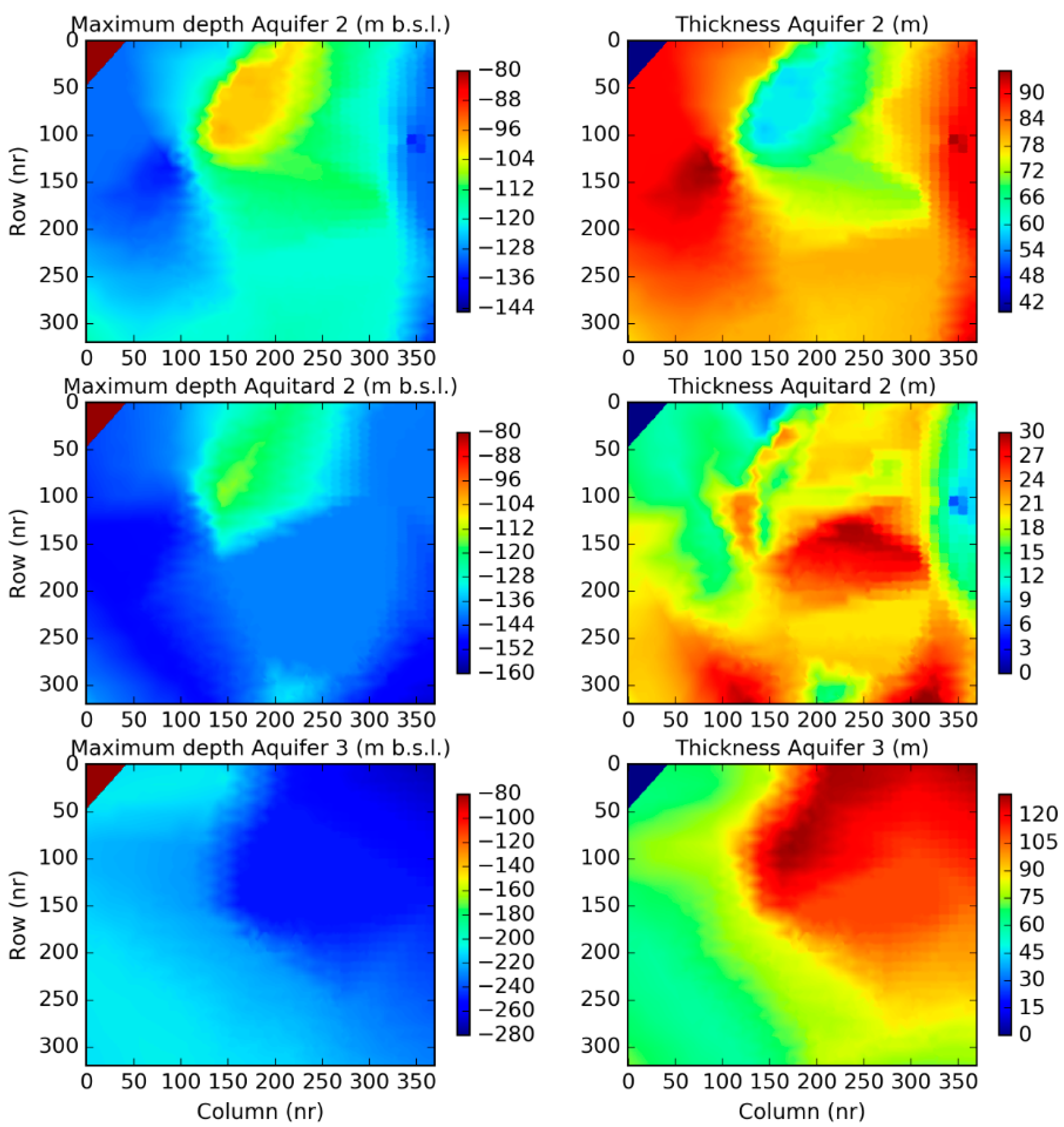
Numerous ASRRO systems to supply freshwater in the greenhouse area were modelled to assess the cumulative impacts on hydrological processes further away from the systems (such as saltwater intrusion) and to assess the relative impact of the application of ASRO and BWRO on its current scale with respect to the whole groundwater system. The 3D Regional Model (18 × 16.5 km) covers the Westland groundwater system (Figure 1). The model is based on the PZH (Province of Zuid-Holland) model used and described in earlier studies [10,18]. The main model parameters are shown in Table 3. Dispersivity and diffusion coefficients are equal to the Local Model. Horizontal cell dimensions are 50 × 50 m. Layer thicknesses are constant in the top 80 m BSL, and vary spatially at greater depths (Figure A1). This results in 1,439,904 active cells. The clay cap confining the upper aquifer (Aquifer 1) is 1 to 3 model layers thick (Figure A2). Aquifer 1 is 3 to 5 model layers thick. The Regional Model’s vertical conductivity (Kv) depends on the horizontal conductivity (Kh). The vertical Kh/Kv-anisotropy equals 10 if the Kh is equal to or below 1 m/day, 3 if the Kh is 1 to 10 m/day, and 2 if the Kh is in between 10 and 30 m/day. Grid cells with a higher Kh have been made isotropic. The Kh and Kv distribution of the Phreatic layer, Aquifer 1, and Aquifer 2 are shown as supplementary information (Figure A3 and Figure A4), as well as the Kh of the Clay Cap and Aquitard 1 (Figure A5).
Constant heads were assigned to both the top layer and the vertical boundary planes (Figure A6). The model bottom is a no-flow boundary, since this was considered to be the hydrological base. No constant concentrations were assigned. Starting concentrations and heads decrease landwards, where deep polders are present and groundwater has lower salinities (for more information, Figure A7 and Figure A8).
The BWRO and ASRRO scenarios include 616 ASRRO wells and 616 MC disposal wells in a grid. ASRRO wells are placed in Aquifer 1 at 20–35 m BSL, 500 m apart. MC disposal wells are placed in Aquifer 2 at 50–80 m BSL, 250 m downstream of each accompanying ASRRO or BWRO well. The annual freshwater injection and recovery equals 8885 m3/year/MPPW, corresponding to a 4.5-ha greenhouse surface per MPPW, which is considered realistic based on comparable existing ASR systems further inland [4]. The durations of injection, storage, and recovery periods are similar to the Local Model. In total, a net volume of 5,473,000 m3 of freshwater is produced from Aquifer 1 during both ASRRO and BWRO each year. This is ca. 0.4% and 0.1% of the pore water volume present in Aquifer 1 (1.46 km3) and Aquifer 2 (5.38 km3), respectively. This means that the ratio of produced versus present groundwater is 11 and 16 times less than in the 27-ha subsection of the Local Model in Aquifer 1 and Aquifer 2, respectively.
3. Results
3.1. Local Impacts of ASRRO and BWRO
3.1.1. Relative Concentration Changes and Concentration Profiles
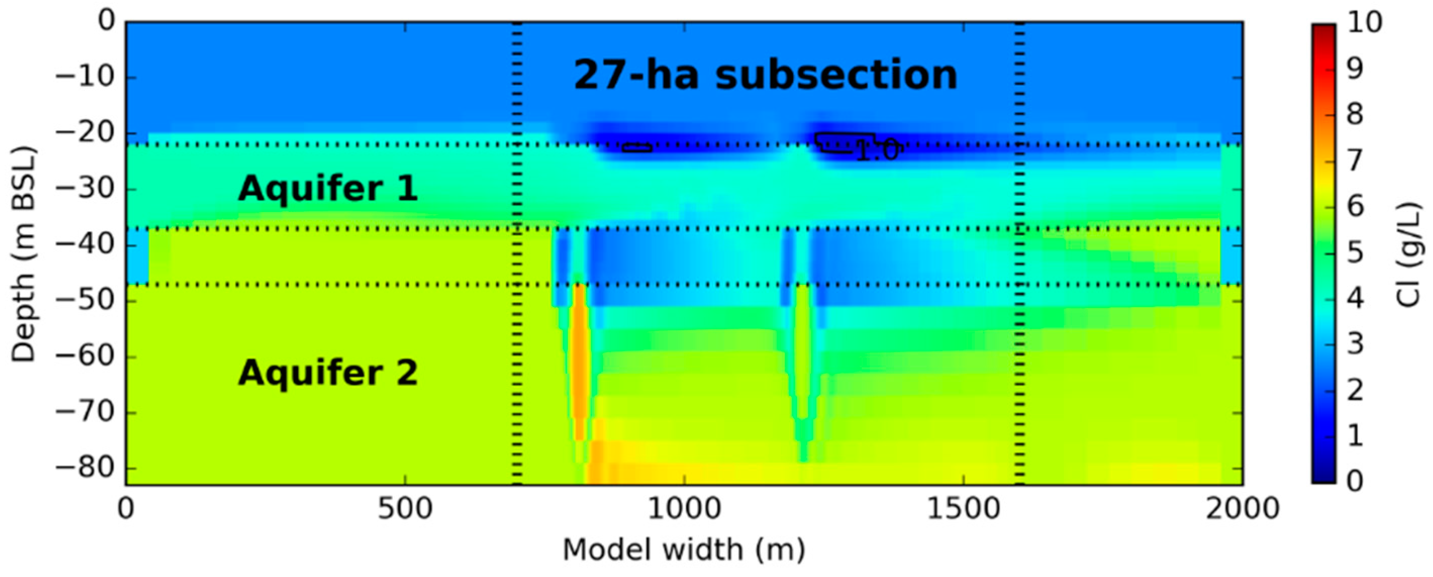
The absolute and relative concentration changes in the 27-ha subsection for ASRRO and BWRO are given in Table 4 and Figure 4 In the autonomous scenario, slow salinization was observed, primarily in the clay layers. Applying ASRRO decreased the subsection’s average salinity with 3.7% with respect to the autonomous situation. The formation of an extensive saltwater plume around the MC disposal wells was not observed during ASRRO (Figure 5). During the first part of each summer abstraction, the injected MC was less saline than the ambient groundwater and subsequently moved upwards through Aquitard 1. Near the end of recovery stages, however, the MC was relatively saline and sank to the basal part of Aquifer 2. Unrecoverable injected freshwater moved upwards in Aquifer 1 and was trapped below the Clay cap. Although stratification in groundwater qualities was introduced during ASRRO, the overall effect on the groundwater quality is neutral to positive.
BWRO in combination with local MC disposal by MC disposal wells increased the average salinity by 15.5% with respect to the autonomous situation (Table 4). Saltwater plumes formed and merged around the MC disposal wells in Aquifer 2, obtaining a combined length of 1200 m and width of 300 m in 30 years (Figure 6). During BWRO, Aquifer 1 suffered from upconing of saline groundwater from Aquifer 2. This was marked by an increase in the chloride concentration of the abstracted RO feed water from 4.3 to 5 to 6 g/L and can be also seen in Figure 6 by the higher salinities at the base of Aquifer 1 near the BWROs in the 27 ha subsection. Outside the 27-ha subsection, changes were limited. The overall impact of BWRO on the groundwater system based on the outcomes is negative due to the general salinization introduced.
3.1.2. Concentration of the Membrane Concentrate
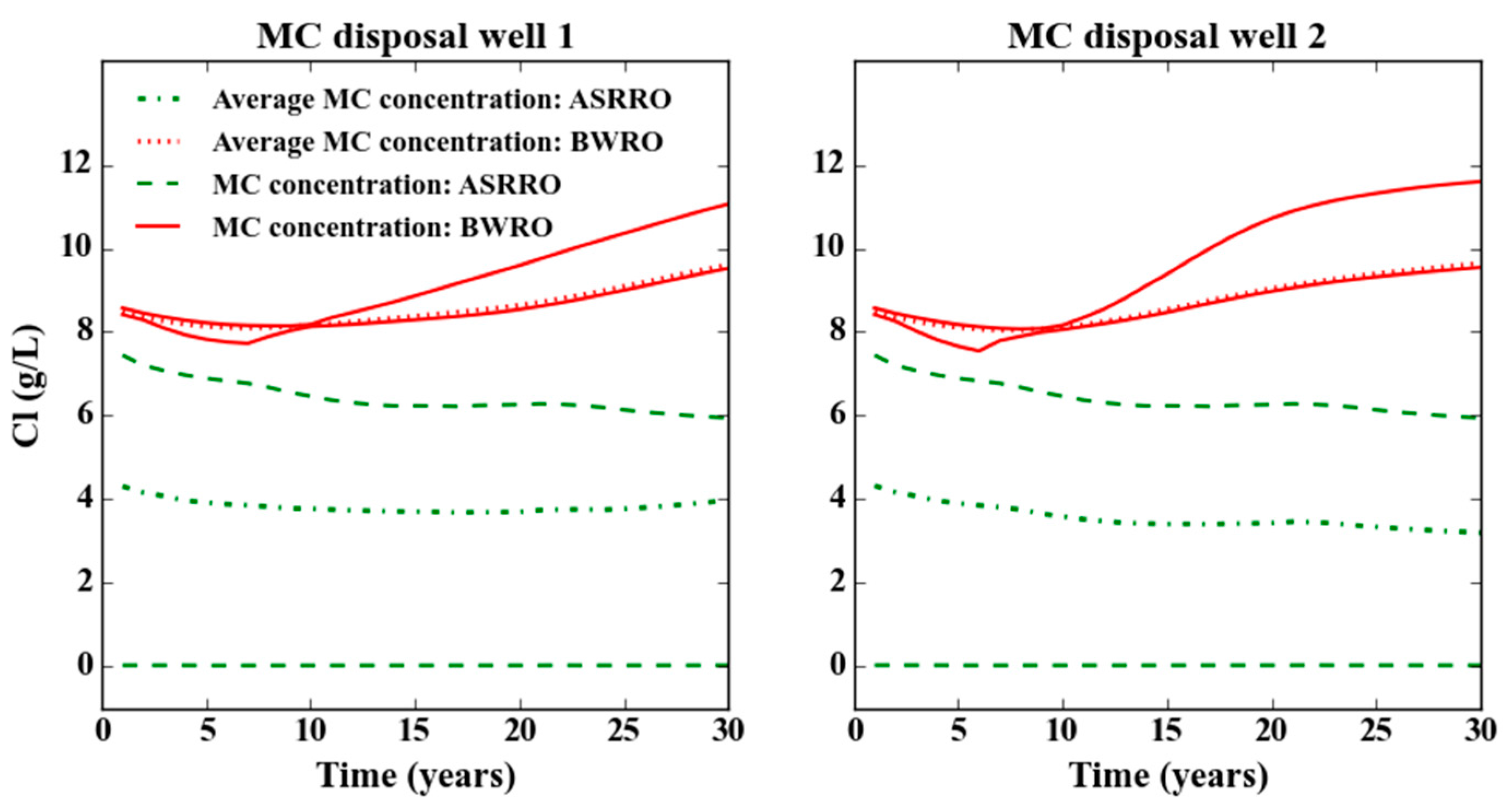
During ASRRO, MC concentrations were initially close to zero and increased to >6 g/L in the final stages of MC injection (Figure 7). On average, the concentration of the disposed water (Cl: 3–4 g/L) was below the initial chloride concentration of Aquifer 2 (6.0 g/L). The water quality of MC reinjected by the downstream MC disposal well 2 (Cl: 3.6 g/L) was slightly better than for MC disposal well 1 (Cl: 3.8 g/L). The injected chloride mass during ASRRO was 47% to 63% lower compared to the BWRO case. In the BWRO case, therefore, disposal of MC by the MC disposal wells (Cl: 7.5–11.6 g/L) significantly exceeded the ambient chloride concentration in Aquifer 2, which was 6 g/L. The average MC disposal concentrations were 8.6 g/L (MC disposal well 1) and 8.7 g/L (MC disposal well 2).
3.2. Regional Impacts of Wide-Spread Implementation of ASRRO and BWRO
3.2.1. Regional Concentration Changes and Concentration Profiles
Modelling the wide-spread implementation of ASRRO and BWRO in a regional model enabled analyses of the cumulative effects on the groundwater system. The average chloride concentrations of the ASRRO and BWRO scenarios after 30 years are shown in Table 5). Both ASRRO (−0.3%) and BWRO (0.0%) had a minor effect on the average chloride concentration in the whole regional groundwater system, which can be related to the fairly limited freshwater production from the aquifer compared to the modelled domain. ASRRO led to a limited freshening of the Clay cap and Aquifer 1, but lowered the average chloride concentration within Aquifer 2 by 1.0%. BWRO decreased the average chloride concentration in the Clay cap and Aquifer 1, while increasing the concentrations in Aquitard 1. A concentration increase (+0.2%) was observed in Aquifer 2, which was targeted for MC injection.
The averaged chloride concentrations after 30 years are given for the grid cells containing the 616 MPPWs or abstraction wells in Aquifer 1 (Figure 8) and MC disposal wells in Aquifer 2 (Figure 9). The average chloride concentration in the autonomous scenario was 1.8 g/L and 5.2 g/L near the MPPWs and MC disposal wells, respectively. ASRRO decreased local chloride concentrations near the wells in Aquifer 1 by 0.7 g/L (−41%) and by 1.0 g/L in Aquifer 2 (−20%) with respect to autonomous scenario, causing a shift to lower salinity classes. In the vicinity of the MC disposal wells of the ASRRO systems, concentrations were in the narrow range of 1.5–4.5 g/L Cl (Figure 9).
In the BWRO scenario, local chloride concentrations in the grid cells of the abstraction wells in Aquifer 1 decreased with 0.3 g/L (−18%) with respect to the autonomous situation and with 0.2 g/L near the MC disposal wells (−3%). The concentrations near the MC disposal wells of BWRO systems were predominantly in the range of 2.5–6 g/L, with a clear peak around 3.0–4.5 g/L Cl, whereas in the autonomous scenario these concentrations were generally in the range of 1.5 to 6.5 g/L Cl (Figure 9).
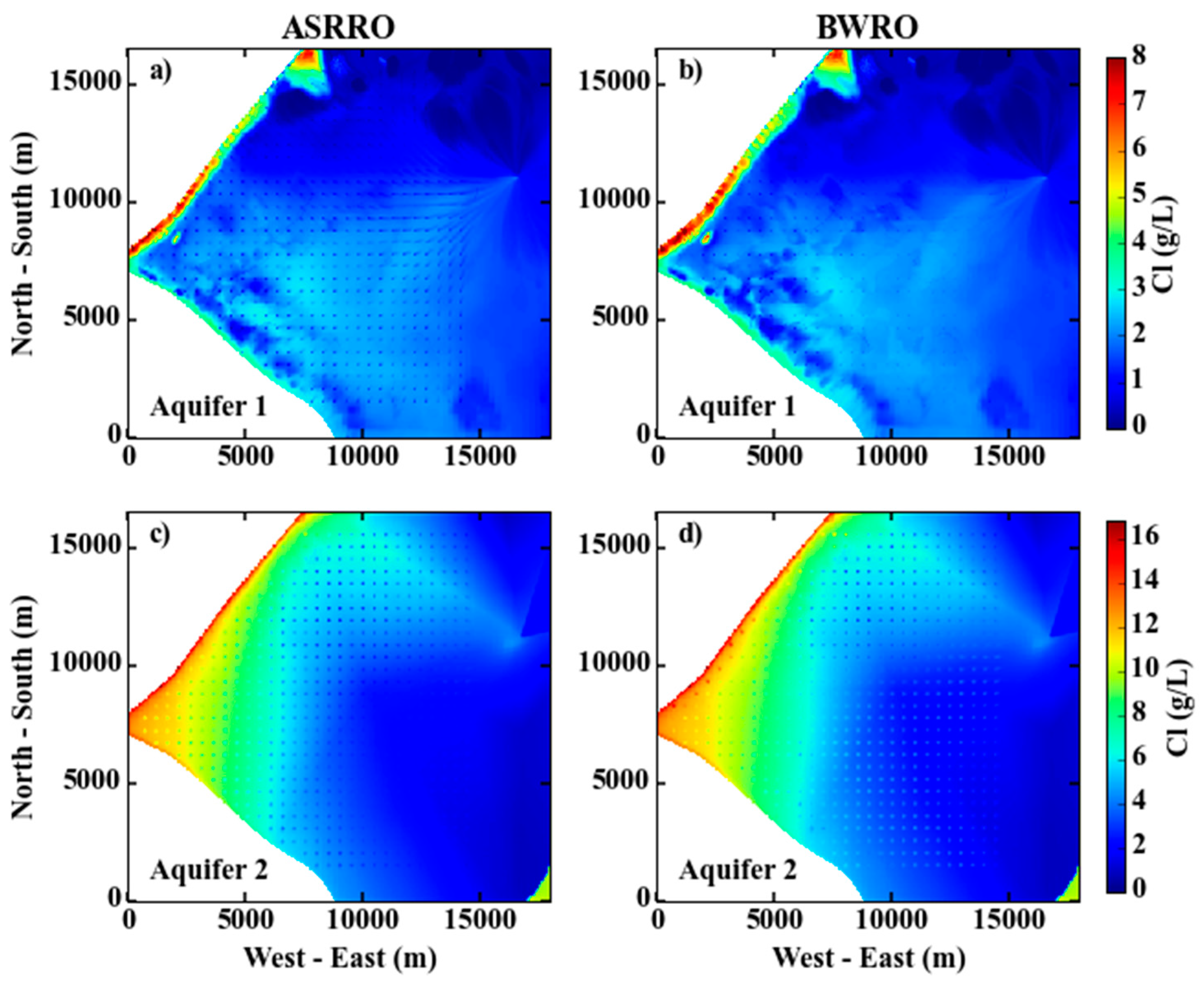
Chloride concentration changes in Aquifer 1 and 2 at the end of the 30-years simulations for both ASRRO and BWRO with respect to the autonomous situation are shown in Figure 10. The absolute concentrations are presented as Figure A9. The impact of the BWRO and ASRRO systems is still relatively local after 30 years. However, ASRRO systems significantly reduced the salinization of Aquifer 2 that was locally occurring during BWRO. Differences were less pronounced within Aquifer 1. Here, it was clear that ASRRO led to less saltwater intrusion along the North Sea shore, as indicated by a narrower strip with strong salinization.
3.2.2. Concentration of the Membrane Concentrate
A distribution of the MC injection water concentration by the MCDWs is presented in Figure 11. The MC injected in Aquifer 2 had an average concentration of 3.6 g/L (in case of BWRO) and 2.1 g/L (in case of ASRRO).
4. Discussion
4.1. Impact of ASRRO on the Groundwater System
The timescale and resolution of the impact of ASRRO on the groundwater systems are significantly different on a local scale (vicinity of the system) and a regional scale (a regional groundwater system). Therefore, the impact on both scales is discussed separately.
4.1.1. Local Impacts on Groundwater Quality
Stratification of Freshwater-Saltwater by ASRRO
Besides impacting the average chloride concentration in the various geological layers, the ASRRO systems heavily impacted the distribution of concentrations in the vertical dimension of the aquifers (‘stratification’). In Aquifer 1, injected freshwater moved to the top and remained where it formed local freshwater lenses. When such lenses merge, they can form a horizontal barrier for saline seepage, similar to vertical barriers along a coastline [19]. As a consequence, the diffuse saline seepage was replaced by freshwater seepage. The second consequence was that MC injected in Aquifer 2 was relatively fresh in the first stages of disposal. This freshwater moved upwards, replacing ambient brackish groundwater in Aquifer 2 and Aquitard 1, also in the downstream direction. Once this water reached Aquifer 1, it diluted the RO feed water of the downstream ASRRO system (MPPW c and d), which can be considered a positive impact.
Relative Impact of ASRRO
Based on the salt budgets of the Local Model, a positive impact of ASRRO on the groundwater system can be derived (Table 4). Ultimately, the total salt mass present during ASRRO in the vicinity of the wells stabilized, apart from seasonal variations caused by freshwater injection and abstraction, indicating that a local salinity equilibrium can be attained. ASRRO systems in the Local Model decreased the total chloride mass in the arbitrary 27-ha subsection by 3.9% with respect to the autonomous situation and caused long-term freshening within the Clay cap, Aquitard 1, and Aquifer 2. Upstream of and lateral to the ASRROs, short-circuiting increased the rate of salinization of Aquitard 1 because of the net abstraction in Aquifer 1, which was required to feed the RO system with sufficient brackish water. This is indicated by a long-term increase in chloride mass in Aquifer 1. Only initially there was a positive impact because of the initial release of relatively fresh groundwater from Aquitard 1. The relative impact of ASRRO on Aquifer 1 can therefore be negative with respect to the autonomous situation (no abstractions). The MC did obtain a lower average chloride concentration (Cl: 3.8 g/L (MC disposal well 1) and 3.6 g/L (MC disposal well 2)) within Aquifer 2 (Figure 9) than in the autonomous situation (Cl: 6.0 g/L) and Aquifer 2 is therefore positively affected. This was due to the annual freshwater injection that locally diluted the groundwater in Aquifer 1 in the vicinity of the MPPWs (Figure 8). The balance between freshwater infiltration and freshwater abstraction is therefore expected to be vital for the total impact of ASRRO on the groundwater system.
Comparing the Impact of BWRO and ASRRO
In the Local Model, ASRRO decreased the total chloride mass in the 27-ha subsection by 16.8% with respect to BWRO and caused relative freshening of the groundwater system (Figure 4). This is regarded a positive impact. In the current practice of BWRO, short-circuiting from Aquifer 2 to Aquifer 1 is more severe than with ASRRO. As a consequence, BWRO intensified the rate of salinization in Aquifer 2 once relatively fresh groundwater from Aquitard 1 was consumed and replaced by relatively saline groundwater from Aquifer 2. As this water reached the MPPWs, the resulting MC became significantly more saline, forming extensive saline water plumes (Cl: 8–12 g/L). This is a negative impact of BWRO and was not observed during ASRRO. No freshwater barrier was formed because of BWRO, but seepage of brackish water towards the surface water system in summer was at least significantly reduced due to the abstraction—and therefore lower heads—in Aquifer 1.
The most noticeable positive impact of ASRRO with respect to BWRO is the absence of a relative salinity increase (and mineral saturation) in the deeper groundwater system. This is however a boundary condition for a long-term use of this groundwater system for freshwater supply, either by ASR (as increasing salinities lower the recovery efficiency [20]) or BWRO (as increasing salinities make BWRO more expensive and energy-consuming [21,22]).
4.1.2. Regional Impacts on Groundwater Quality
Widespread use of ASRRO in the Regional Model decreased the average regional chloride concentration by 0.3%, which can be considered a positive impact. The total impact on the groundwater system is significantly less due to the lower ratio of produced freshwater versus present groundwater (Section 2.2.1). BWRO resulted in higher average chloride concentrations of 0.2% with respect to ASRRO (Table 5). However, because of the net abstraction of groundwater in Aquifer 1 during ASRRO as well, additional saltwater intrusion still occurred along the coastline (Figure 10). This can be considered a negative impact of ASRRO. Yet still, this intrusion is significantly reduced when it is compared to the modelled intrusion caused by the current, wide-spread use of BWRO. In Aquifer 2, on the other hand, the MC disposal resulted in a transformation of saltwater intrusion to an outflow of brackish water towards the sea (Figure 12).
The abstractions for BWRO increased the infiltration of relatively fresh groundwater from the Clay cap and decreased Aquifer 1 concentrations regionally, as occurred in the first 10 years of the BWRO application in the Local Model. The positive effects of increased infiltration even outweighed those resulting from freshwater injection by ASRRO. Infiltration of freshwater from the surface may be exaggerated in this study by the modelling approach, in which constant heads and constant low salinities (freshwater) were assigned to the whole phreatic layer.
In the Regional Model, the MC disposal wells were further away from the brackish water abstraction wells than in the Local Model (250 m instead of 50 m), while each system had a lower capacity (8885 m3/system/year instead of 27,000 m3/system/year). This limited the rate of short-circuiting from Aquifer 2 to Aquifer 1 and reduced the local effects. However, once short-circuiting becomes prominent—as in the pilot [10]—salinization of abstraction wells will occur, which can undo this initially positive development (Figure 12). Short-circuiting should therefore be regarded a major obstacle for (long-term) use of BWRO in the study area.
In the Westland regional model, BWRO did not negatively affect chloride concentrations around each individual abstraction and MC disposal well. This depended on the local initial salinity of Aquifer 1 and 2 and the chosen RO recovery of 50%. Moreover, as with ASRRO, the disposal of MC into Aquifer 2 reduced salt water intrusion. This may imply that potentially no negative effects or even freshening may be observed when concentrations in Aquifer 2 are locally double or more than double the concentrations in Aquifer 1 (western and central parts of the Westland: Figure 10), unless short-circuiting occurs due to a limited separation of both aquifers. In such a case, it is relevant to analyse if this is really a sustainable situation, or that the net abstraction still results in saltwater intrusion in (parts of) the area, and thus, eventually, in salinization of the abstraction well. This risk is also present with ASRRO, albeit smaller due to the winter freshwater injections. Careful planning of wells will be beneficial to the limitation of rapid and severe local effects, although it will not influence the regional effects. Altogether, the regional impact of BWRO seems acceptable, but is strongly dependent on enhanced natural infiltration and sufficient spreading of BWRO systems.
4.2. Implications of This Study for the Use of the Westland Groundwater System and Coastal Groundwater Systems Elsewhere
In the Westland area, the net abstraction during BWRO results in enhanced infiltration and saltwater intrusion, which was shown by this study. Excessive long-term decreasing groundwater tables are therefore not observed in the area and the predominant effects of water mining are the increasing salinities in the aquifers. Therefore, the current solution for high-quality irrigation water supply in the Westland area (BWRO) is under its hydrogeological conditions an unsustainable water supply solution and leads to slow mining of remnant (relatively) fresh water and saltwater intrusion [23], which is marked as an undesired effect upon exploitation of groundwater systems. Unlike falling groundwater levels, the slow salinization process is difficult to observe and will manifest itself primarily by a slow increase of the salt mass in the groundwater system and of the salinity of the abstracted brackish water. This eventually makes BWRO a less efficient or even infeasible technique.
A switch to ASRRO will prevent or limit the impact on the groundwater body of using the Westland’s aquifers as an irrigation water source and may therefore be preferred from a policy point of view, taking into account European Water Framework Directive and especially the European Groundwater Directive [24], as they set specific goals for the condition of groundwater bodies. A boundary condition for success is the balance between (artificial) infiltration of freshwater surpluses and freshwater production during ASRRO. Positive side effects can be a reduction of subsidence and the intentional lowering of water levels in of aboveground rainwater reservoirs by infiltration for enhanced retention during intensive rainfall events.
Hurdles for large-scale implementation of ASRRO to mitigate potential impacts on the groundwater body may be the variability of the water demand in the area, however. Horticulturists with a low water demand can suffice with an aboveground rainwater reservoir, whereas horticulturists with a high water demand require more water than available by precipitation. On average, these imbalances can be eliminated in the Westland due to the equal volumes of water surplus and demand over time, but there is currently no incentive for horticulturists with a low water demand to infiltrate their surplus. A water bank [25] may provide a potential governance instrument to overcome this hurdle. A technical hurdle can be the mobilisation of particles upon freshening [26,27], which can lead to clogging of RO membranes during ASRRO [28]. The extent to which this process occurs and potential mitigation strategies are relevant fields of future research.
The Westland coastal groundwater system suffers from many typical water related issues observed in coastal zones worldwide, the most important ones being saltwater intrusion, subsidence, sea level rise, salinization of surface waters, and an increasing water quality and quantity demand, especially during prolonged droughts. The Westland case can therefore be considered a valuable example for improvement of the management of coastal groundwater systems with ASRRO. However, several local operational (e.g., infiltrated and recovered volumes) and hydrogeological (e.g., aquifers, aquitards, drainage levels, nearby abstractions) controlling factors will affect the overall impact and their cumulative impact on any groundwater system. This overall impact should therefore be evaluated before widespread ASRRO implementation in other areas.
5. Conclusions
In this study, the expected impacts of combined aquifer storage and recovery and reverse osmosis (ASRRO) on the water quality of the Westland groundwater system have been assessed through modelling the local effects of ASRRO and effects of widespread ASRRO implementation.
ASRRO reduces the salinities in its vicinity. An initially local, horizontal freshwater barrier forms at the top of the ASRRO target aquifer (Aquifer 1) and the aquifer for MC disposal (Aquifer 2), positively impacting seepage by lowering its salinity. In the deepest interval of Aquifer 2, a plume with slightly increased salinities can form and migrate downstream. However, this plume is significantly smaller compared with brackish water reverse osmosis (BWRO: the current practice, in which no rainwater is injected). In this case, an overall increase in the system’s salinization rate was observed. During BWRO, increasingly more saline water will enter Aquifer 2, thereby forming an increasingly large and significantly more saline plume and creating the risk for upconing towards the brackish water abstraction wells in Aquifer 1.
Regionally, both ASRRO and BWRO resulted in an increase in saltwater intrusion in the aquifer targeted for freshwater storage and production (Aquifer 1), while in Aquifer 2 the saltwater intrusion was reduced by the outflow of brackish water upon MC disposal. The saltwater intrusion in Aquifer 1 during ASRRO was limited as a consequence of the freshwater injections. Furthermore, the significantly lower MC concentrations during ASRRO in combination with the brackish water outflow towards the sea improved the overall salinity in Aquifer 2. The same outflow was observed during BWRO, but the high concentrations in the MC deteriorated the groundwater quality in that case, such that a water quality improvement of Aquifer 2 was not attained.
The outcomes of this study highlight the complex interplays when targeting coastal groundwater systems with freshwater supply techniques like ASRRO and BWRO. Based on this case study, an overall positive to neutral impact of ASRRO on a coastal groundwater system is presumed, which is an improvement with respect to the use of BWRO in the same setting. ASRRO thus provides means to sustainably use coastal groundwater systems. However, several operational (e.g., infiltrated and recovered volumes) and hydrogeological (e.g., aquifers, aquitards, drainage levels, nearby abstractions) controlling factors will affect the overall impact and their cumulative impact on any groundwater system and should be considered before ASRRO implementation elsewhere.
Acknowledgments
The authors would like to thank the funding agent of this study: the EU FP7 project ‘Demonstrate Ecosystem Services Enabling Innovation in the Water Sector’ (DESSIN, grant agreement no. 619039). We thank Deltares for kindly providing the relevant datasets of the PZH model. We sincerely thank two anonymous reviewers and the editor of MDPI Water for their helpful suggestions to improve the manuscript.
Author Contributions
Steven Eugenius Marijnus Ros and Koen Gerardus Zuurbier conceived and designed the modeling experiments; Steven Eugenius Marijnus Ros performed the modeling; Steven Eugenius Marijnus Ros and Koen Gerardus Zuurbier analyzed the data and wrote the paper.
Conflicts of Interest
The authors declare no conflict of interest. The founding sponsors had no role in the design of the study; in the collection, analyses, or interpretation of data; in the writing of the manuscript, and in the decision to publish the results.
Appendix A. Model Input Regional Model
Figure A1.
Maximum depth of occurrence (m below surface level) and total thickness (m) of Aquifer 2 (top), Aquitard 2 (middle), and Aquifer 3 (bottom).
Figure A1.
Maximum depth of occurrence (m below surface level) and total thickness (m) of Aquifer 2 (top), Aquitard 2 (middle), and Aquifer 3 (bottom).

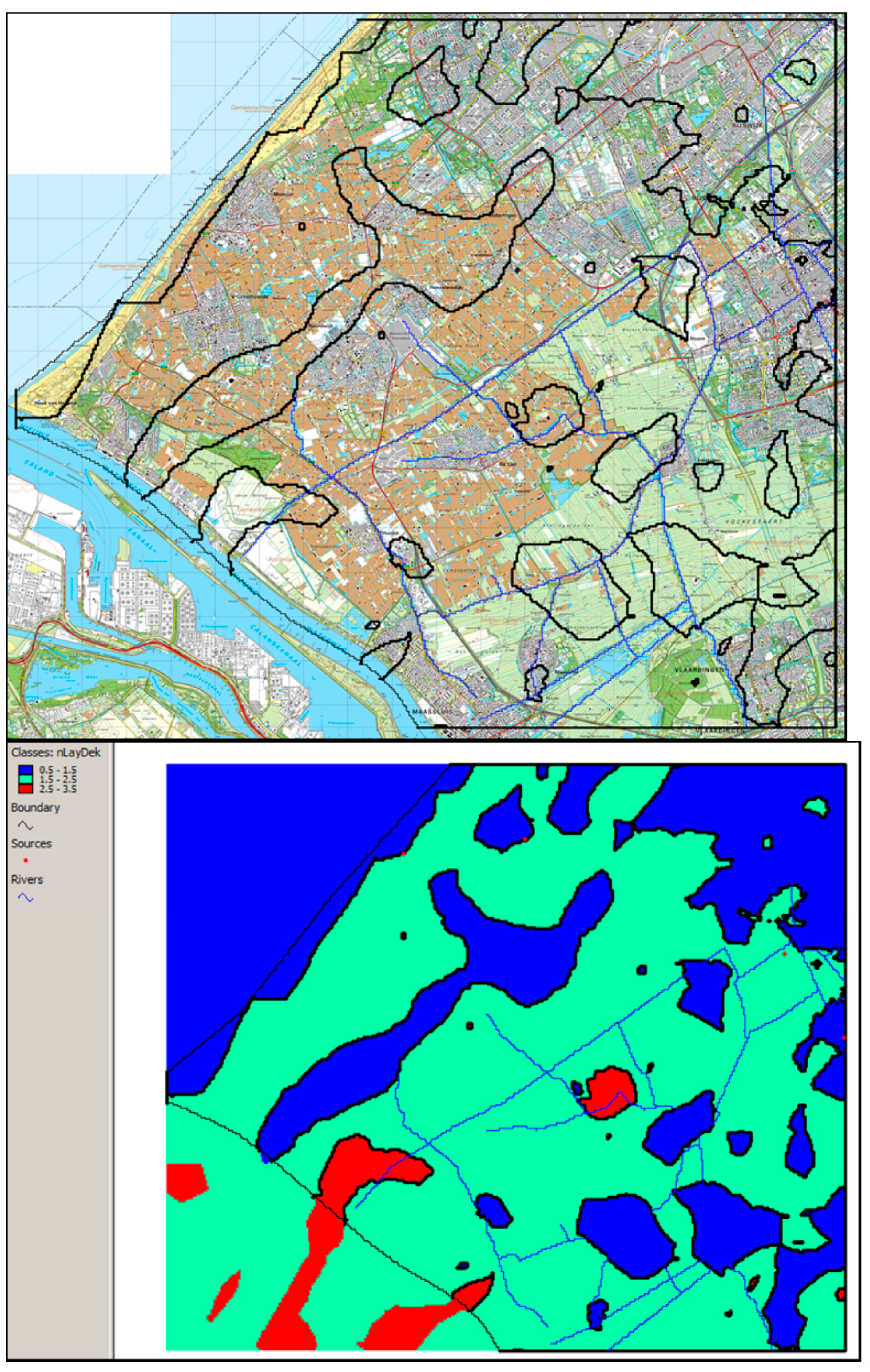
Figure A2.
Topographic map (top) showing the outline of the regions wherein the Holocene clay cap is either 1, 2 or 3 model layers thick. The latter is presented in the bottom figure. The clay cap occurs in L2, (L3, L4), and is at most 15 m thick. The clay layer occurrence has been obtained from the PZH-Westland data [18].

Figure A3.
Horizontal conductivities (m/day) in the Regional Model for the Phreatic layer, and Aquifers 1 and 2. The North Sea is located northwest of the model domain.
Figure A3.
Horizontal conductivities (m/day) in the Regional Model for the Phreatic layer, and Aquifers 1 and 2. The North Sea is located northwest of the model domain.
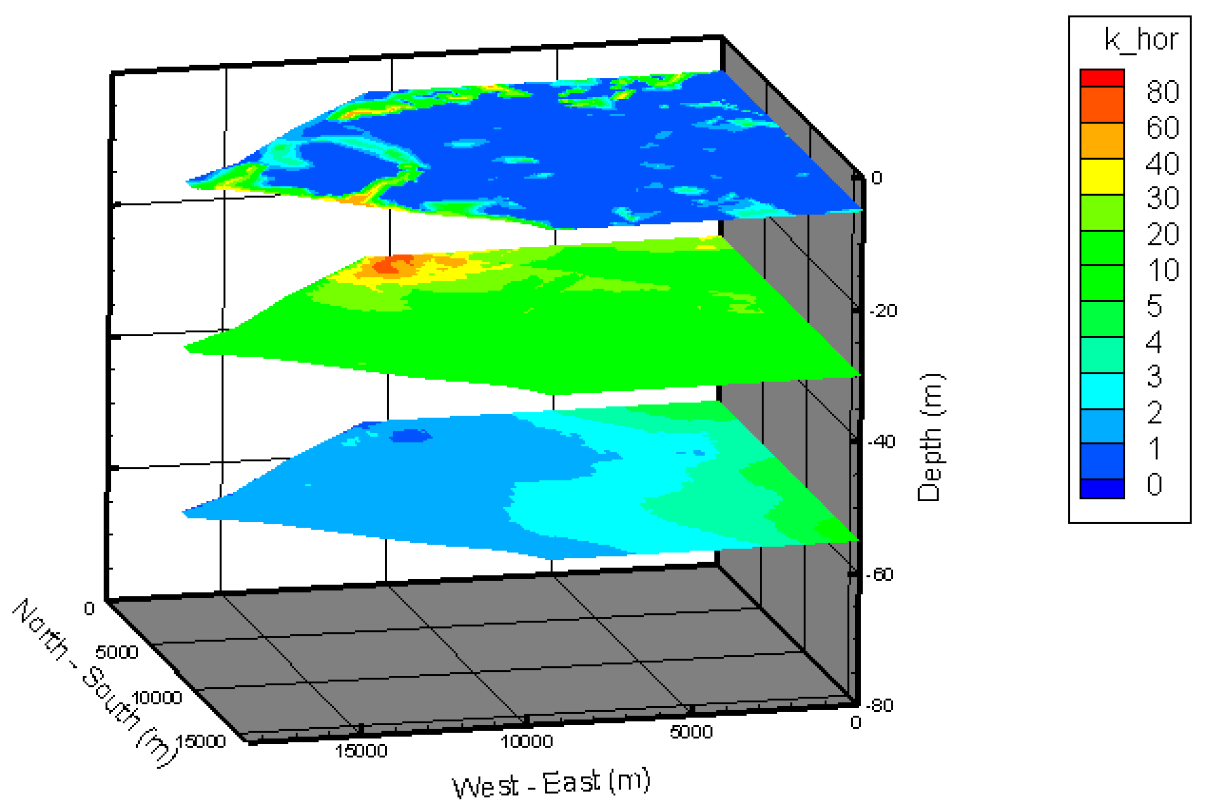
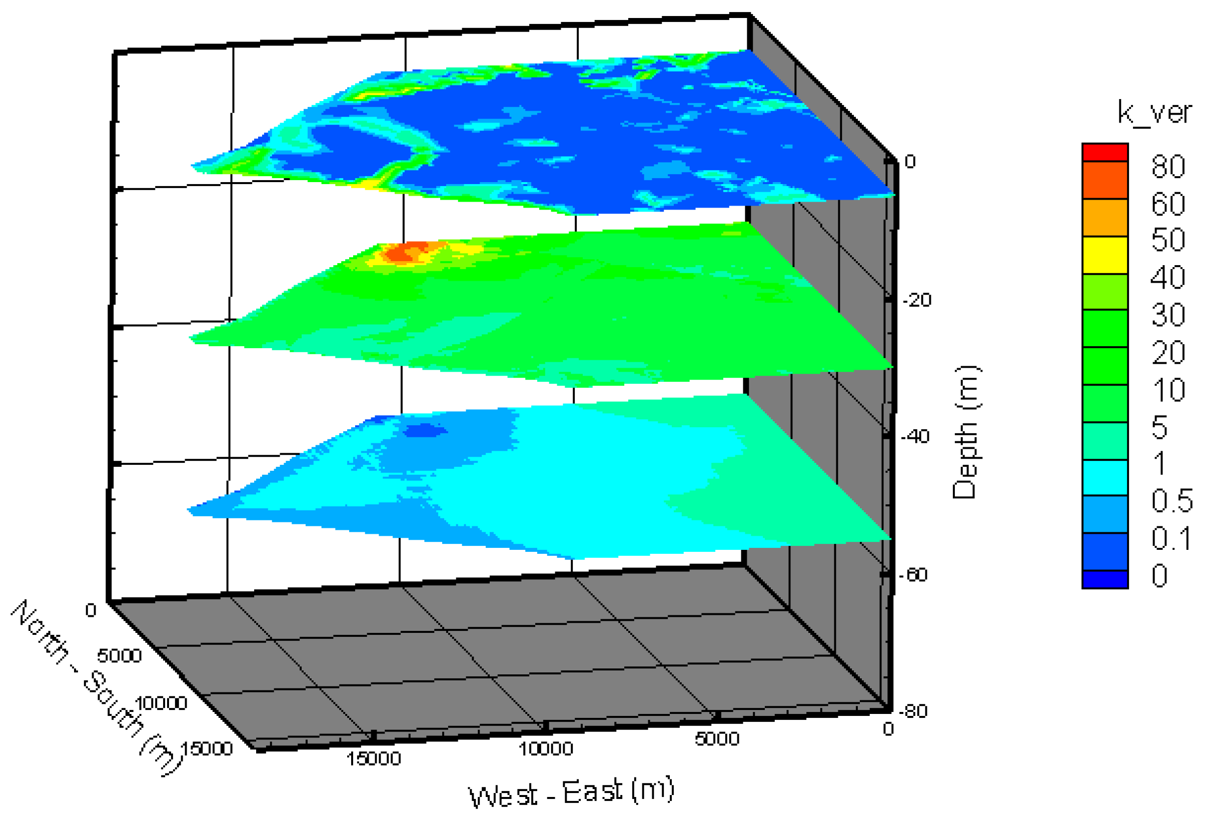
Figure A4.
Vertical conductivities (m/day) in the Regional Model for the Phreatic layer, and Aquifers 1 and 2. The North Sea is located northwest of the model domain.
Figure A4.
Vertical conductivities (m/day) in the Regional Model for the Phreatic layer, and Aquifers 1 and 2. The North Sea is located northwest of the model domain.

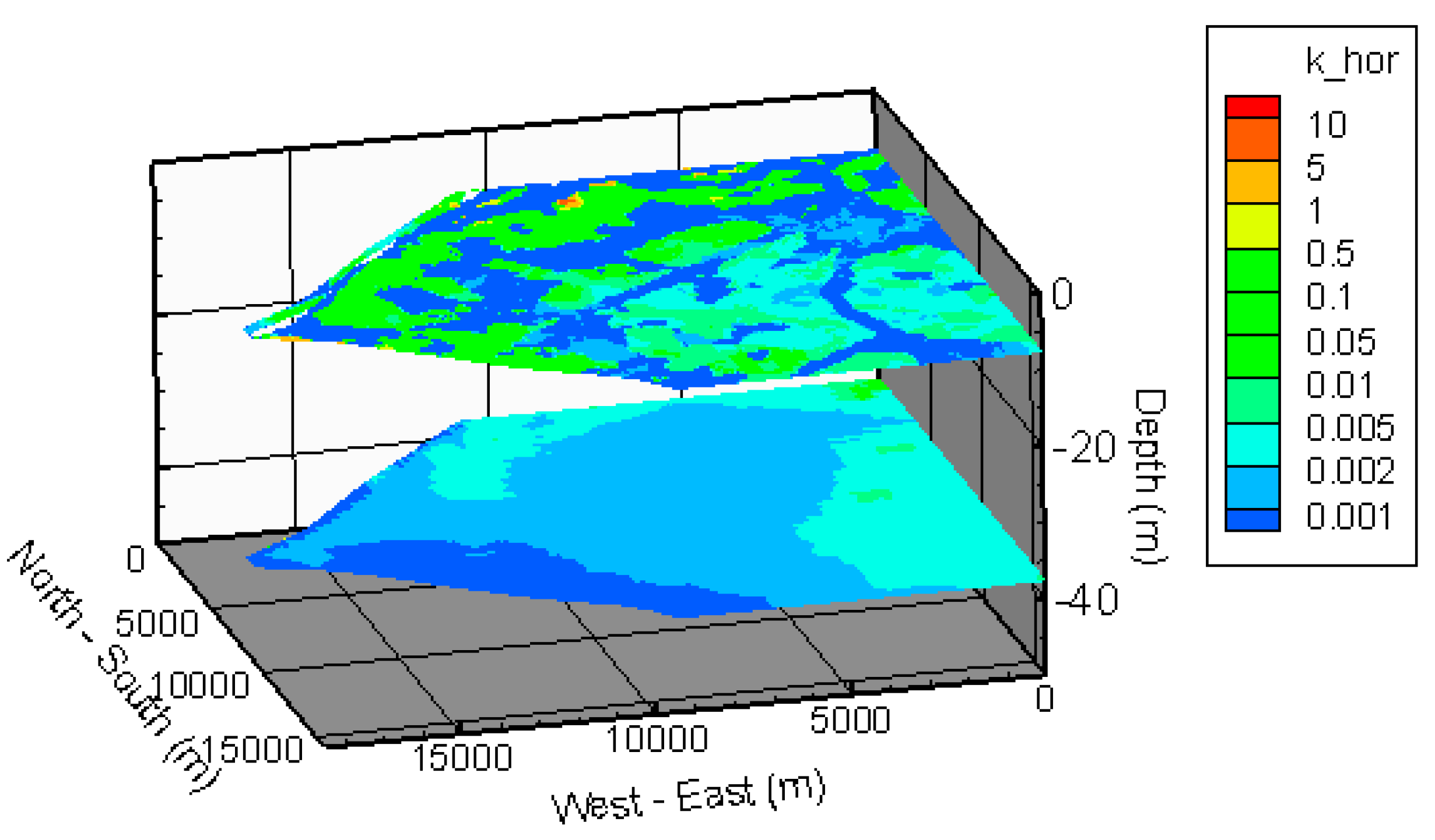
Figure A5.
Horizontal conductivities (m/day) in the Regional Model for the Clay cap and Aquitard 1. The North Sea is located northwest of the model domain.
Figure A5.
Horizontal conductivities (m/day) in the Regional Model for the Clay cap and Aquitard 1. The North Sea is located northwest of the model domain.

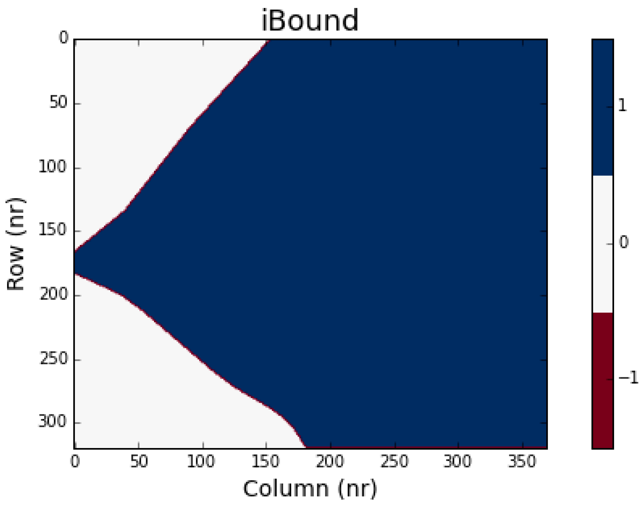
Figure A6.
iBounds (−1, 0, 1) used in the Regional Model. The values are set to “−1” along the vertical boundary planes surrounding the active grid cells and in the top layer.
Figure A6.
iBounds (−1, 0, 1) used in the Regional Model. The values are set to “−1” along the vertical boundary planes surrounding the active grid cells and in the top layer.

Figure A7.
Starting concentrations (g/L) in the Regional Model for the Phreatic layer, and Aquifers 1 and 2. The North Sea is located northwest of the model domain.
Figure A7.
Starting concentrations (g/L) in the Regional Model for the Phreatic layer, and Aquifers 1 and 2. The North Sea is located northwest of the model domain.
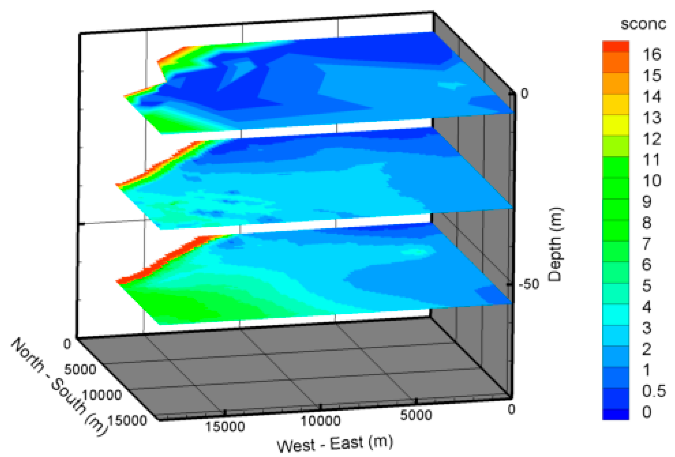
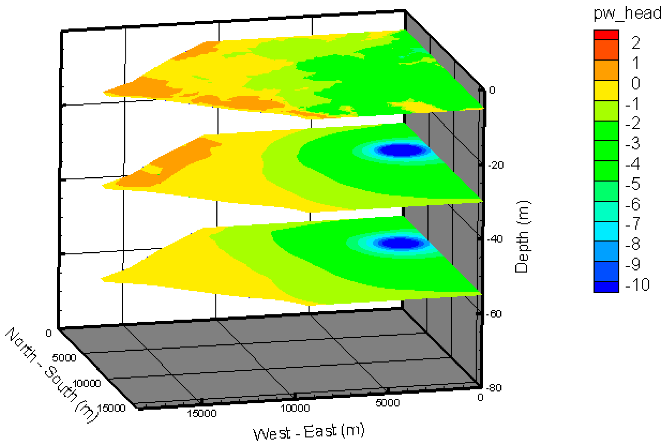
Figure A8.
Point water heads (m) in the Regional Model for the Phreatic layer, and Aquifers 1 and 2. The North Sea is located northwest of the model domain.
Figure A8.
Point water heads (m) in the Regional Model for the Phreatic layer, and Aquifers 1 and 2. The North Sea is located northwest of the model domain.

Figure A9.
Chloride concentration (g/L) after 30 years of practice of ASRRO and BWRO in Aquifer 1 (a,b) and Aquifer 2 (c,d).
Figure A9.
Chloride concentration (g/L) after 30 years of practice of ASRRO and BWRO in Aquifer 1 (a,b) and Aquifer 2 (c,d).
References
- Maliva, R.G.; Missimer, T.M. Aquifer Storage and Recovery and Managed Aquifer Recharge using wells: Planning, hydrogeology, design and operation. In Methods in Water Resources Evolution; Schlumberger: Houston, TX, USA, 2010; 578p. [Google Scholar]
- Pyne, R.D.G. Aquifer Storage Recovery: A guide to Groundwater Recharge through Wells; ASR Systems LLC: Gainesville, FL, USA, 2005; 608p. [Google Scholar]
- Stuyfzand, P.; Raat, K. Benefits and hurdles of using brackish groundwater as a drinking water source in the Netherlands. Hydrogeol. J. 2010, 18, 117–130. [Google Scholar] [CrossRef]
- Zuurbier, K.; Bakker, M.; Zaadnoordijk, W.; Stuyfzand, P. Identification of potential sites for aquifer storage and recovery (ASR) in coastal areas using ASR performance estimation methods. Hydrogeol. J. 2013, 21, 1373–1383. [Google Scholar] [CrossRef]
- Esmail, O.J.; Kimbler, O.K. Investigation of the technical feasibility of storing fresh water in saline aquifers. Water Resour. Res. 1967, 3, 683–695. [Google Scholar] [CrossRef]
- Merritt, M.L. Recovering Fresh Water Stored in Saline Limestone Aquifers. Ground Water 1986, 24, 516–529. [Google Scholar] [CrossRef]
- Ward, J.D.; Simmons, C.T.; Dillon, P.J.; Pavelic, P. Integrated assessment of lateral flow, density effects and dispersion in aquifer storage and recovery. J. Hydrol. 2009, 370, 83–99. [Google Scholar] [CrossRef]
- Van Ginkel, M.; Olsthoorn, T.N.; Bakker, M. A New Operational Paradigm for Small-Scale ASR in Saline Aquifers. Groundwater 2014, 52, 685–693. [Google Scholar] [CrossRef] [PubMed]
- Oosterhof, A.; Raat, K.J.; Wolthek, N. Reuse of salinized well fields for the production of drinking water by interception and desalination of brackish groundwater. In Proceedings of the 9th Conference on Water Reuse, Windhoek, Namibia, 27–31 October 2013; International Water Association (IWA): London, UK, 2013. [Google Scholar]
- Zuurbier, K.G.; Stuyfzand, P.J. Consequences and mitigation of saltwater intrusion induced by short-circuiting during aquifer storage and recovery (ASR) in a coastal subsurface. Hydrol. Earth Syst. Sci. Discuss. 2017, 21, 1173–1188. [Google Scholar] [CrossRef]
- Zuurbier, K.G.; Haas, K.; Huiting, H. Assessment Reversed Osmosis Membrane Clogging by Varying Redox Conditions of Feedwater; KWR Watercycle Research Institute: Nieuwegein, The Netherlands, 2016. [Google Scholar]
- Oude Essink, G.H.P.; van Baaren, E.S.; de Louw, P.G.B. Effects of climate change on coastal groundwater systems: A modeling study in the Netherlands. Water Resour. Res. 2010, 46, W00F04. [Google Scholar] [CrossRef]
- Zuurbier, K.G.; Zaadnoordijk, W.J.; Stuyfzand, P.J. How multiple partially penetrating wells improve the freshwater recovery of coastal aquifer storage and recovery (ASR) systems: A field and modeling study. J. Hydrol. 2014, 509, 430–441. [Google Scholar] [CrossRef]
- Langevin, C.D.; Thorne, D.T.; Dausman, A.M.; Sukop, M.C.; Guo, W. SEAWAT version 4: A computer program for simulation of multi-species solute and heat transport. In Techniques and Methods, Book 6; USGS, Ed.; Geological Survey (U.S.): Reston, VA, USA, 2007. [Google Scholar]
- Bakker, M. FloPy3. 2016. Available online: http://modflowpy.github.io/flopydoc/introduction.html (accessed on 30 October 2016).
- Appelo, C.A.J.; Postma, D. Geochemistry, Groundwater and Pollution, 2nd ed.; A.A. Balkema: Leiden, The Netherlands, 2005; 649p. [Google Scholar]
- Paalman, M. Enlarging Selfsufficient Horticultural Freshwater Supply: Greenhouse Areas Haaglanden (Part 1); KvK105/2013A; Knowledge for Climate: Utrecht, The Netherlands, 2012. (In Dutch) [Google Scholar]
- Faneca Sànchez, M.; Raat, K.J.; Klein, J.; Paalman, M.; Oude Essink, G. Effects of Concentrate Disposal on the Groundwater Quality and Functions in the Westland Area; KWR: Nieuwegein, The Netherlands, 2012; 70p. (In Dutch) [Google Scholar]
- Luyun, R.; Momii, K.; Nakagawa, K. Effects of Recharge Wells and Flow Barriers on Seawater Intrusion. Ground Water 2011, 49, 239–249. [Google Scholar] [CrossRef] [PubMed]
- Bakker, M. Radial Dupuit interface flow to assess the aquifer storage and recovery potential of saltwater aquifers. Hydrogeol. J. 2010, 18, 107–115. [Google Scholar] [CrossRef]
- Karagiannis, I.C.; Soldatos, P.G. Water desalination cost literature: Review and assessment. Desalination 2008, 223, 448–456. [Google Scholar] [CrossRef]
- Zhu, A.; Christofides, P.D.; Cohen, Y. Energy Consumption Optimization of Reverse Osmosis Membrane Water Desalination Subject to Feed Salinity Fluctuation. Ind. Eng. Chem. Res. 2009, 48, 9581–9589. [Google Scholar] [CrossRef]
- Werner, A.D.; Bakker, M.; Post, V.E.; Vandenbohede, A.; Lu, C.; Ataie-Ashtiani, B.; Barry, D.A. Seawater intrusion processes, investigation and management: Recent advances and future challenges. Adv. Water Resour. 2013, 51, 3–26. [Google Scholar] [CrossRef]
- The Groundwater Directive. Directive 2006/118/EC of the European Parliament and of the Council of 12 December 2006 on the Protection of Groundwater against Pollution and Deterioration; 2006/118/EC; European Commission: Brussels, Belgium, 27 December 2006. [Google Scholar]
- Dillon, P. Australian progress in managed aquifer recharge and the water banking frontier. Water J. Aust. Water Assoc. 2015, 42, 53–57. [Google Scholar]
- Brown, D.L.; Silvey, W.D. Artificial Recharge to a Freshwater-Sensitive Brackish-Water Sand Aquifer, Norfolk, Virginia; Geological Survey Professional Paper; U.S. Government Publishing Office: Washington, DC, USA, 1977; 53p.
- Konikow, L.F.; August, L.L.; Voss, C.I. Effects of Clay Dispersion on Aquifer Storage and Recovery in Coastal Aquifers. Trans. Porous Media 2001, 43, 45–64. [Google Scholar] [CrossRef]
- Jonsson, G.; Macedonio, F.; Enrico, D.; Lidietta, G. Fundamentals in Reverse Osmosis. In Comprehensive Membrane Science and Engineering; Elsevier: Oxford, UK, 2010; pp. 1–22. [Google Scholar]
Figure 1.
The principle of aquifer storage and recovery and reverse osmosis (ASRRO) for storage and recovery of freshwater in brackish-saline aquifers.
Figure 1.
The principle of aquifer storage and recovery and reverse osmosis (ASRRO) for storage and recovery of freshwater in brackish-saline aquifers.
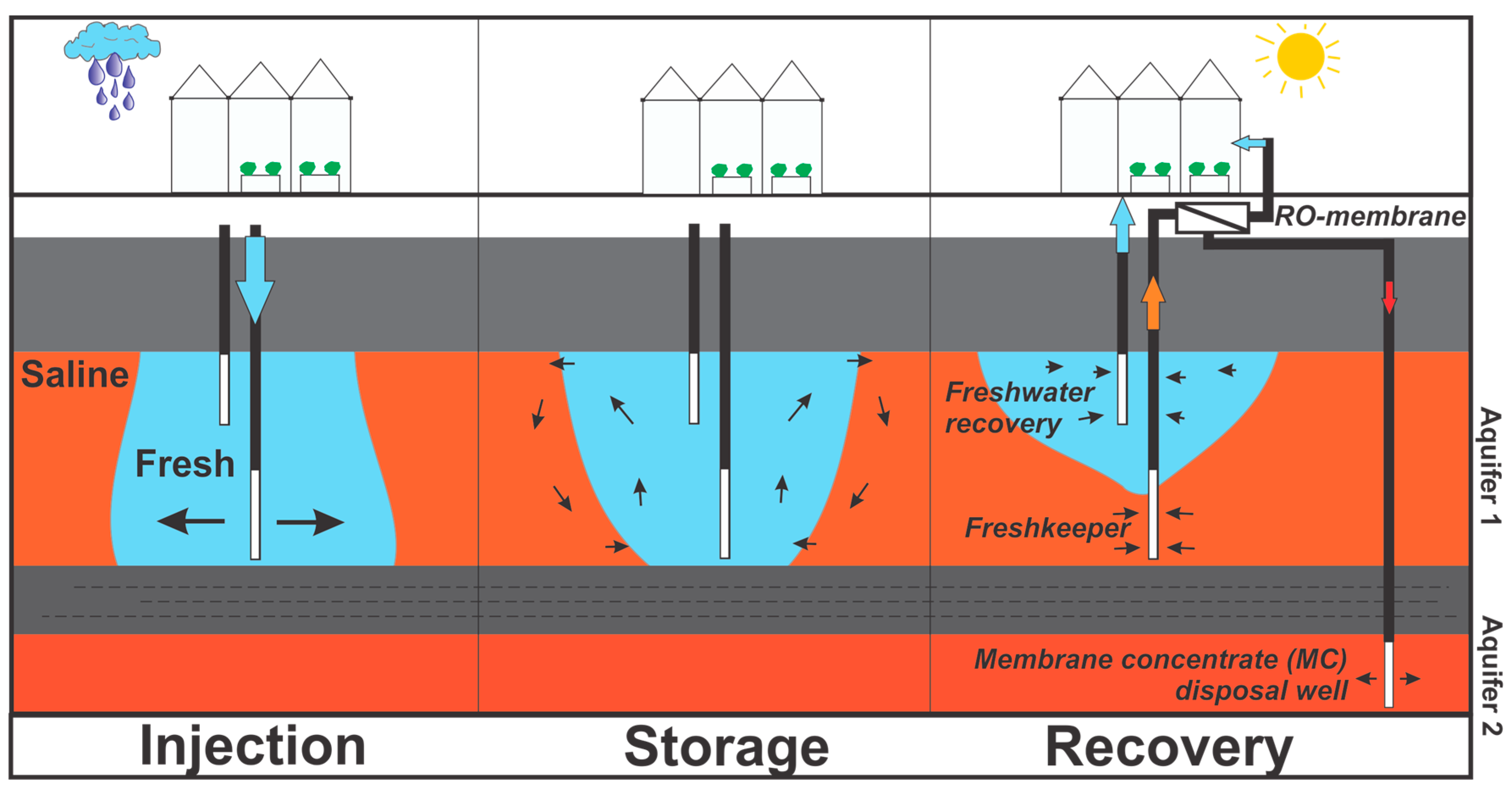
Figure 2.
Location of the Westland study area and the regional hydraulic heads, groundwater salinity, location of greenhouse horticulture, and boundaries of the groundwater models.
Figure 2.
Location of the Westland study area and the regional hydraulic heads, groundwater salinity, location of greenhouse horticulture, and boundaries of the groundwater models.
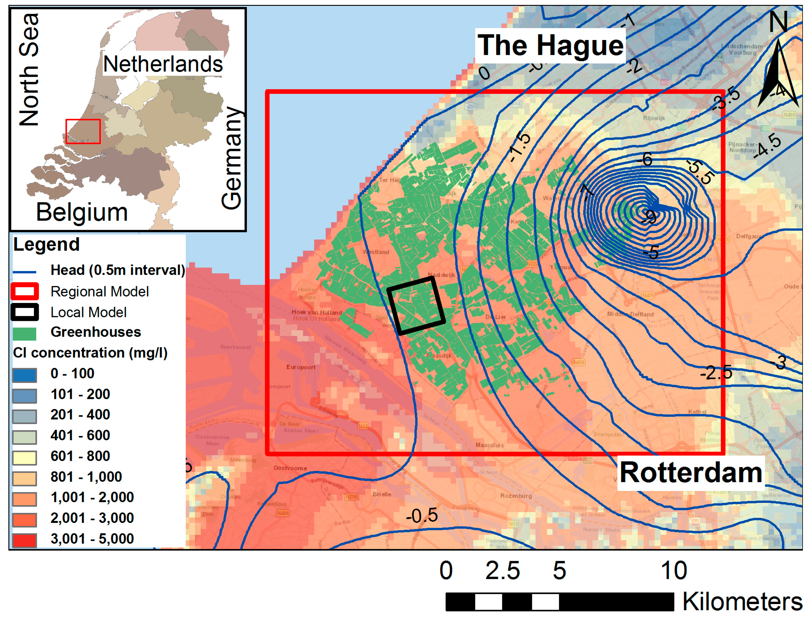
Figure 3.
Top: Top view of the Local Model grid. Bottom: Cross-sectional view (West-East) showing the hydraulic heads (h) and the expected flow pattern through the various geological layers for the autonomous situation. The 27-ha subsection (area of the greenhouses connected to the ASRRO system) of the model is located within the marked box. The vertical exaggeration is 10:1.
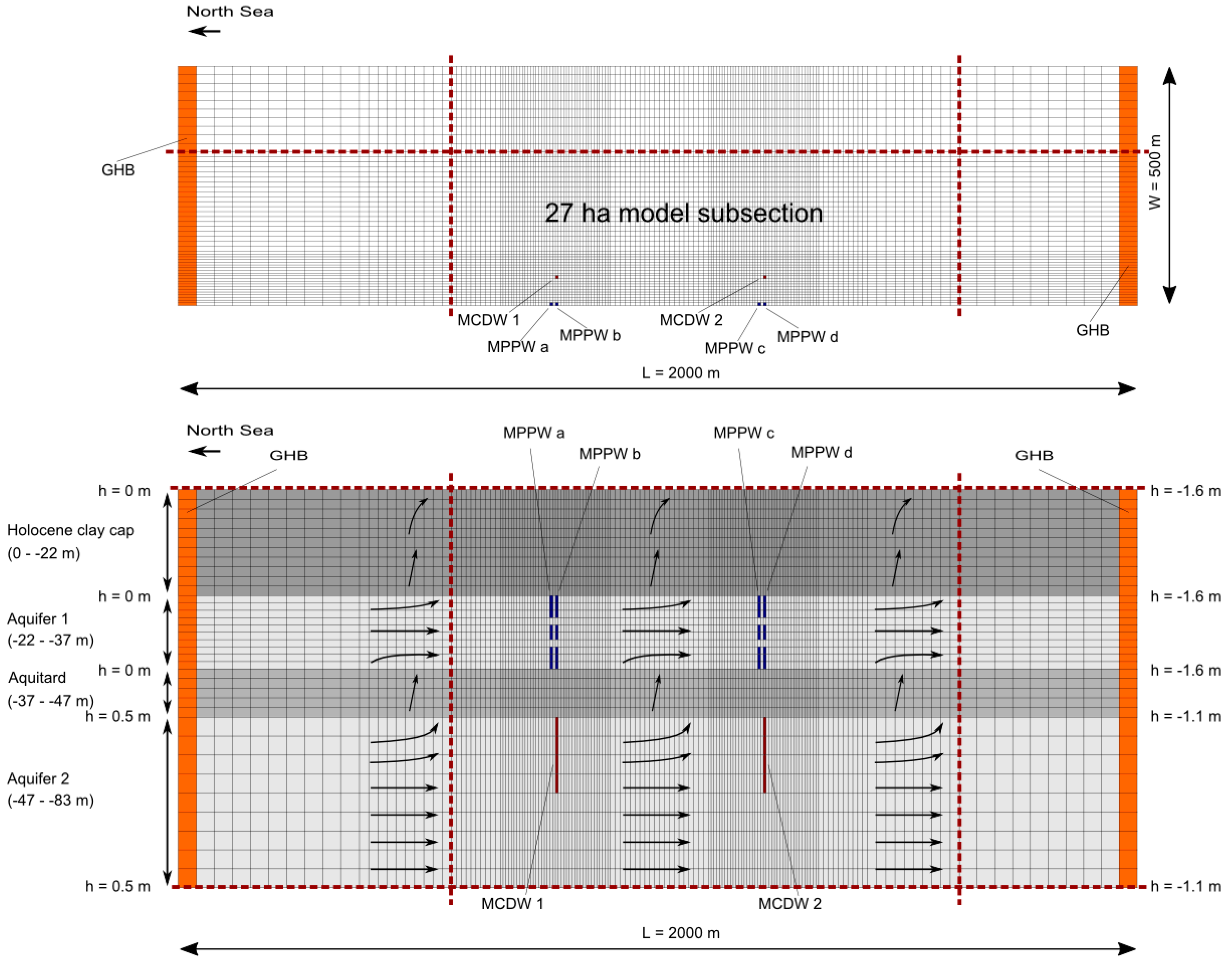
Figure 4.
Average chloride concentration (g/L) throughout the 27-ha model subsection for: the total groundwater system (a), the Clay cap (b), Aquifer 1 (c), Aquitard 1 (d), and Aquifer 2 (e).
Figure 4.
Average chloride concentration (g/L) throughout the 27-ha model subsection for: the total groundwater system (a), the Clay cap (b), Aquifer 1 (c), Aquitard 1 (d), and Aquifer 2 (e).
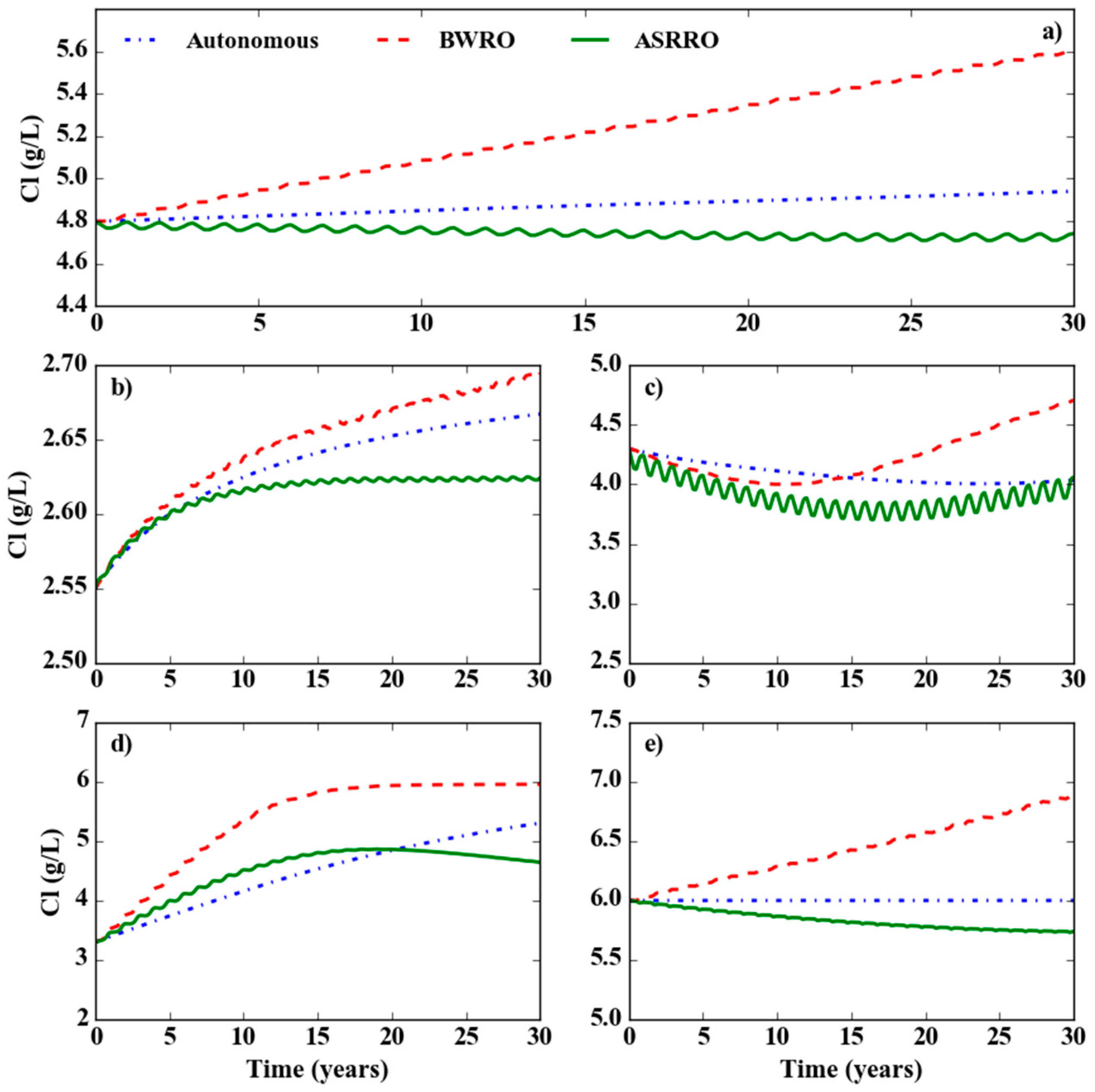
Figure 5.
Chloride concentrations along the mirror plane (W- > E) of Local Model where the MC disposal wells are situated (scenario ASRRO; t = 30 year, end of summer). The 27-ha model subsection includes the part shown between the vertical dotted lines (x = 70; x = 160).
Figure 5.
Chloride concentrations along the mirror plane (W- > E) of Local Model where the MC disposal wells are situated (scenario ASRRO; t = 30 year, end of summer). The 27-ha model subsection includes the part shown between the vertical dotted lines (x = 70; x = 160).

Figure 6.
Chloride concentrations along the mirror plane (W- > E) of the Local Model where the MC disposal wells are situated (scenario BWRO; t = 30 year, end of summer). The 27-ha model subsection includes the part shown between the vertical dotted lines (x = 70; x = 160).
Figure 6.
Chloride concentrations along the mirror plane (W- > E) of the Local Model where the MC disposal wells are situated (scenario BWRO; t = 30 year, end of summer). The 27-ha model subsection includes the part shown between the vertical dotted lines (x = 70; x = 160).
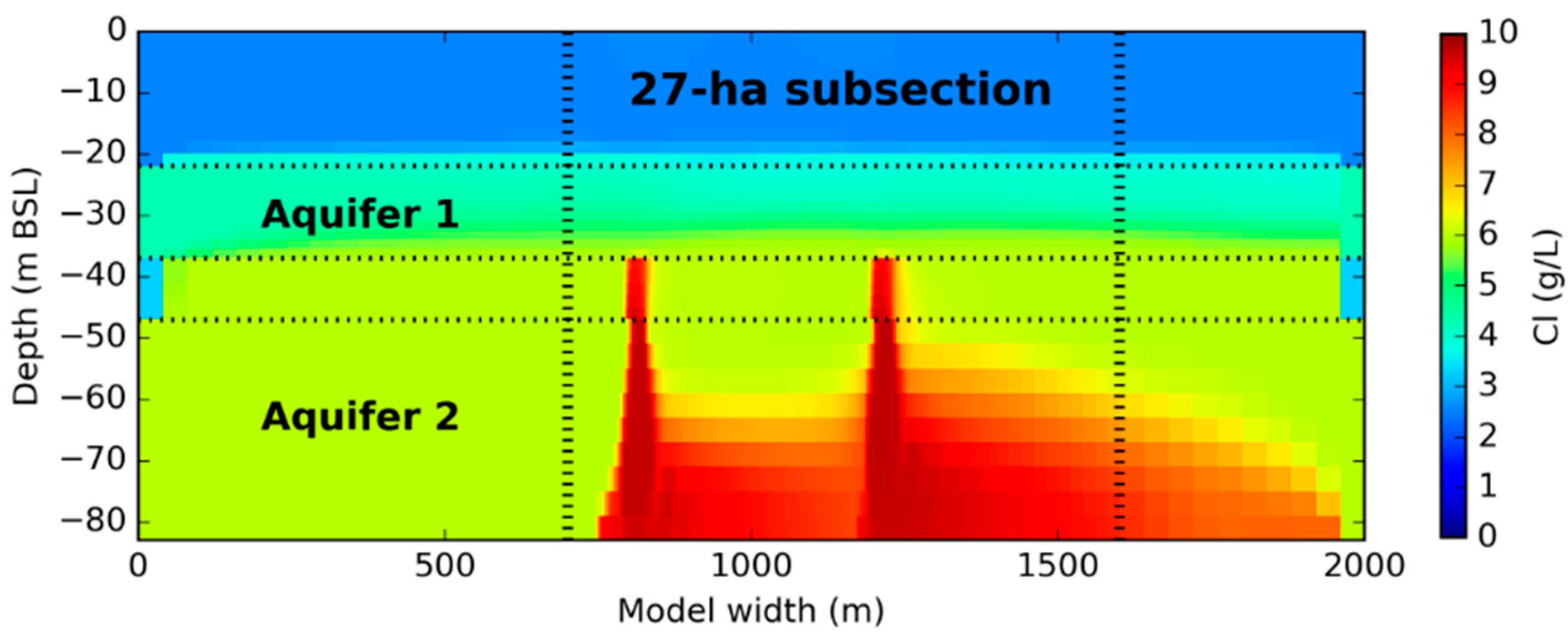
Figure 7.
Range of MC concentrations with time of water injected by MC disposal well 1 and MC disposal well 2, for ASRRO and BWRO; and the yearly averaged MC concentration of each MC disposal well for both scenarios.
Figure 7.
Range of MC concentrations with time of water injected by MC disposal well 1 and MC disposal well 2, for ASRRO and BWRO; and the yearly averaged MC concentration of each MC disposal well for both scenarios.

Figure 8.
Distribution of local chloride concentrations in the 50 m × 50 m model cells of the MPPWs (Aquifer 1) of each individual BWRO and ASRRO system (average during the final year (year 30)).
Figure 8.
Distribution of local chloride concentrations in the 50 m × 50 m model cells of the MPPWs (Aquifer 1) of each individual BWRO and ASRRO system (average during the final year (year 30)).
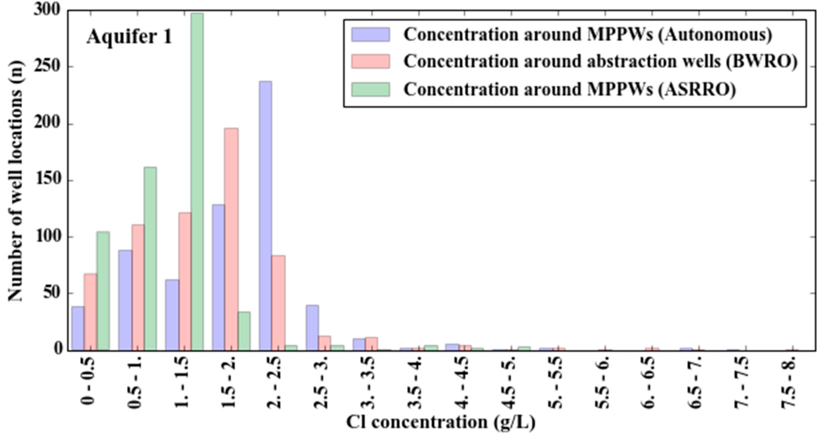
Figure 9.
Distribution of local chloride concentrations in the 50 m × 50 m model cells of the MC disposal wells (Aquifer 2) of each individual BWRO and ASRRO system (average during the final year (year 30)).
Figure 9.
Distribution of local chloride concentrations in the 50 m × 50 m model cells of the MC disposal wells (Aquifer 2) of each individual BWRO and ASRRO system (average during the final year (year 30)).
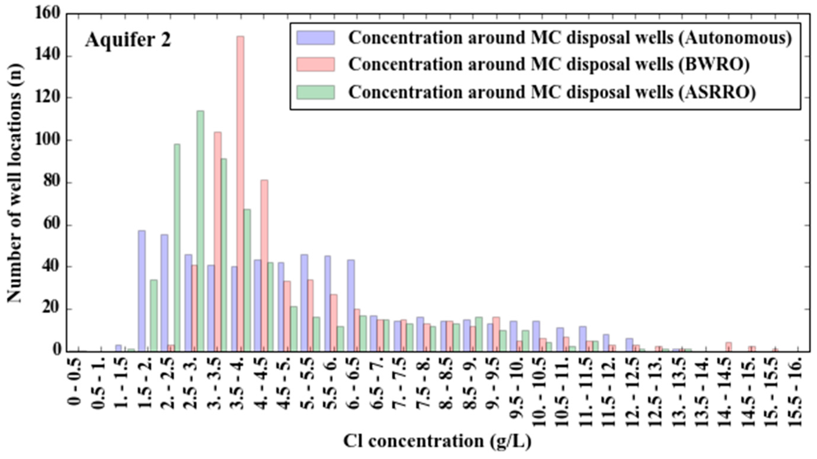
Figure 10.
Relative chloride concentration changes (g/L) between ASRRO and Autonomous and between BWRO and Autonomous after 30 years in Aquifer 1 (a,b) and Aquifer 2 (c,d).
Figure 10.
Relative chloride concentration changes (g/L) between ASRRO and Autonomous and between BWRO and Autonomous after 30 years in Aquifer 1 (a,b) and Aquifer 2 (c,d).
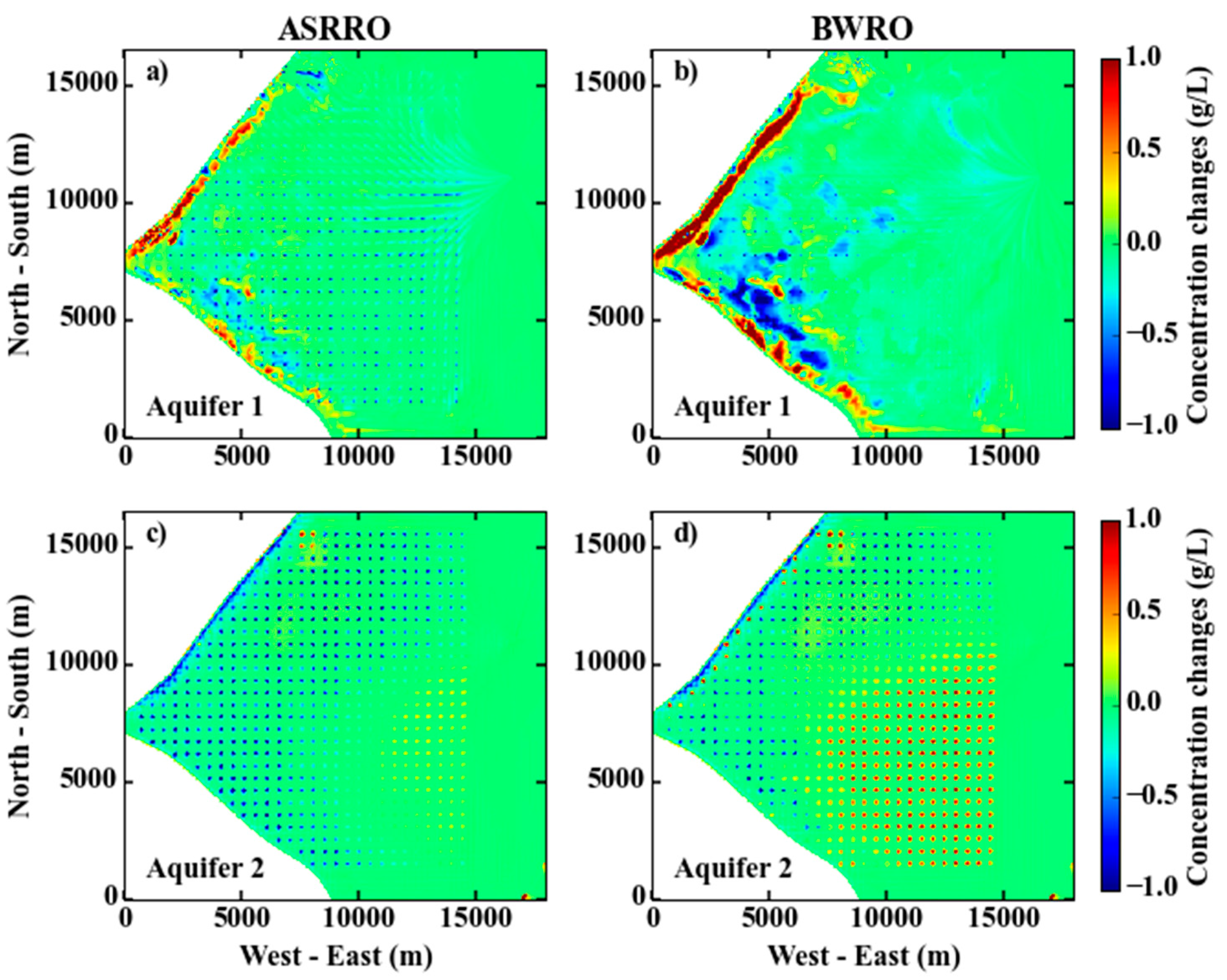
Figure 11.
Distribution of the 30-year averaged MC chloride concentration by the 616 MC disposal wells.
Figure 11.
Distribution of the 30-year averaged MC chloride concentration by the 616 MC disposal wells.
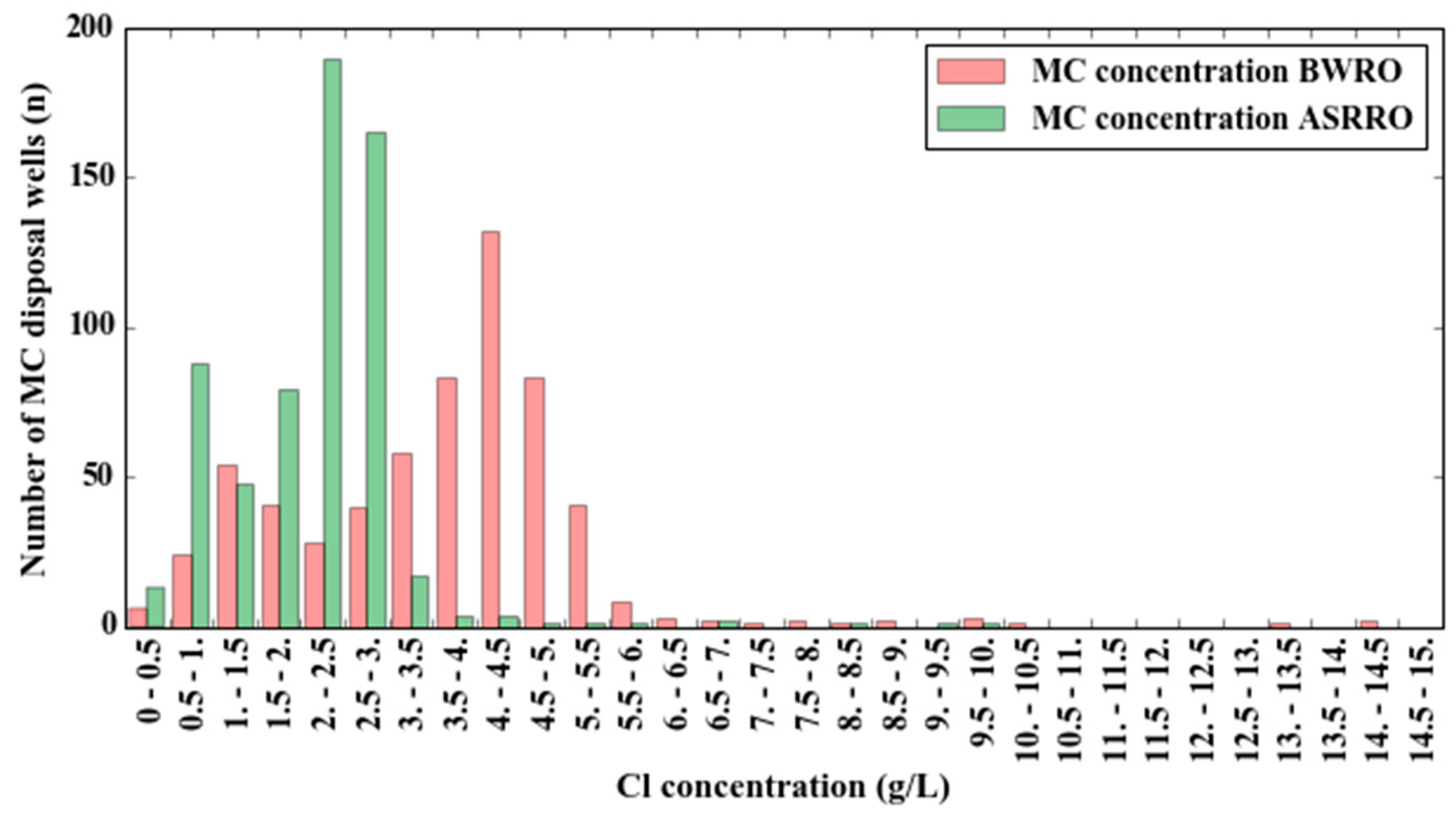
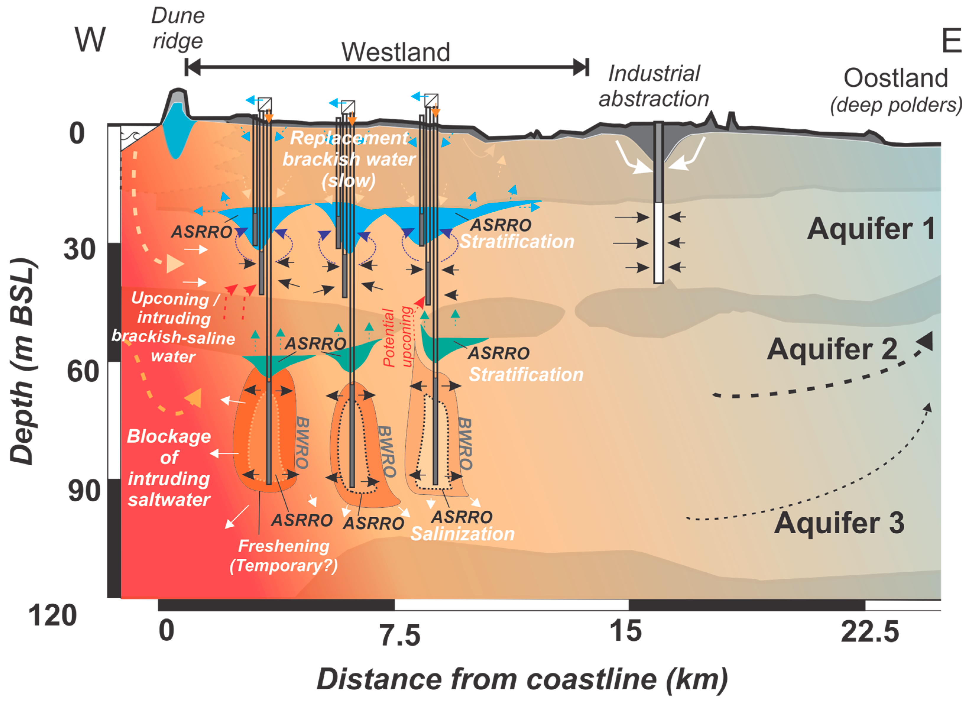
Figure 12.
Overview of the integral impacts of ASRRO (and BWRO) on the regional salinity distribution in the Westland study area in a west-east cross-section. Local impact include salinization (BWRO) and stratification (ASRRO), while regionally saltwater intrusion (Aquifer 1) and brackish water outflow are the main phenomena, having the most negative impact in the BWRO scenario.


Table 1.
Local Model main parameter values.
| Geological Layer | Depth | Layers | Porosity, n | K (Horizontal)/K (Vertical) | Storativity, S | Starting Conc |
|---|---|---|---|---|---|---|
| (m BSL) | (Thickness) | (-) | (m/day) | (-) | Cl (mg/L) | |
| Holocene clay cap | 0–22 | 11 (2 m) | 0.2 | 0.1/0.01 | 0.001 | 2550 |
| Aquifer 1 | 22–37 | 10 (1.5 m) | 0.3 | 35.0/35.0 | 1 × 10⁻⁶ | 4300 |
| Aquitard 1 | 37–47 | 5 (2 m) | 0.2 | 0.2/0.02 | 0.001 | 3300 |
| Aquifer 2 | 47–83 | 9 (4 m) | 0.35 | 30.0/30.0 | 1 × 10⁻⁶ | 6000 |
Table 2.
Operational scheme of each of the 4 MPPWs (a–d) in the Local Model.
| BWRO | Time | Volume | Rate | ASRRO | Time | Volume | Rate |
|---|---|---|---|---|---|---|---|
| (Days) | (m3) | (m3/Day) | (dAys) | (m3) | (m3/Day) | ||
| Idle period | 182 | 0 | 0 | Winter injection | 123 | 13,500 | 109.8 |
| Storage period | 59 | 0 | 0 | ||||
| Summer abstraction | 153 | −13,500 | −88.2 | Summer abstraction | 153 | −13,500 | −88.2 |
| Idle period | 30 | 0 | 0 | Idle period | 30 | 0 | 0 |
Table 3.
Regional Model main parameter values. The * indicates that the number of model layers in which the geological layer is present, is spatially variable. The ‘var’ indicates that the model layer thicknesses vary spatially.
Table 3.
Regional Model main parameter values. The * indicates that the number of model layers in which the geological layer is present, is spatially variable. The ‘var’ indicates that the model layer thicknesses vary spatially.
| Geological Layer | Depth | Layers | Porosity, n | K (Horizontal) | Storativity, S |
|---|---|---|---|---|---|
| (m BSL) | (Thickness) | (-) | (m/Day) | (-) | |
| Phreatic | 0–5 | L1 (5 m) | 0.3 | 0.25–75 | 0.1 |
| Holocene clay cap | 5–20 * | L2–4 (5 m) | 0.3 | <1 | 0.001 |
| Aquifer 1 | 10–35 * | L3–7 (5 m) | 0.3 | 9–75 | 0.001 |
| Aquitard 1 | 35–40 | L8 (5 m) | 0.3 | 0–0.01 | 0.001 |
| Aquifer 2 | 40–135 | L9–10 (5 m), 11–13 (10 m), 14 (var) | 0.3 | 1–5 | 0.001 |
| Aquitard 2 | 100–154 | L15 (var) | 0.3 | 0.001–0.002 | 0.001 |
| Aquifer 3 | 114–272 | L16–17 (var) | 0.3 | 0.1–1 | 0.001 |
Table 4.
Average concentrations within each geological layer throughout the 27-ha subsection after 30 years’ time, for the autonomous situation, ASRRO, and BWRO; the relative concentration increase (in %) of the ASRRO and BWRO cases, and the relative concentration increase (in %) of the ASRRO case compared to BWRO.
| Geological | Autonomous | ASRRO | Rel. Conc | BWRO | Rel. Conc | Rel. Conc Change ASRRO |
|---|---|---|---|---|---|---|
| Layer | Concentration | Concentration | Change ASRRO | Concentration | Change BWRO | Compared to BWRO |
| (g/L) | (g/L) | (%) | (g/L) | (%) | (%) | |
| Clay cap | 2.67 | 2.63 | −1.5 | 2.70 | +1.2 | −2.7 |
| Aquifer 1 | 3.91 | 3.97 | +1.4 | 4.71 | +20.3 | −15.8 |
| Aquitard 1 | 5.07 | 4.60 | −9.3 | 6.03 | +18.7 | −23.6 |
| Aquifer 2 | 6.00 | 5.73 | −4.5 | 6.97 | +16.2 | −17.8 |
| Total | 4.90 | 4.72 | −3.7 | 5.66 | +15.5 | −16.7 |
Table 5.
Average concentrations within each geological layer after 30 years’ time for the Westland_auto, Westland_BWRO, and Westland_ASRRO; the relative concentration increase (in %) of the BWRO and ASRRO cases, and the relative concentration increase (in %) of the ASRRO case compared to BWRO.
Table 5.
Average concentrations within each geological layer after 30 years’ time for the Westland_auto, Westland_BWRO, and Westland_ASRRO; the relative concentration increase (in %) of the BWRO and ASRRO cases, and the relative concentration increase (in %) of the ASRRO case compared to BWRO.
| Geological Layer | Autonomous Concentration | ASRRO Concentration | Rel. Conc Change | BWRO Concentration | Rel. Conc Change | Rel. Conc Change Compared to BWRO |
|---|---|---|---|---|---|---|
| (g/L) | (g/L) | (%) | (g/L) | (%) | (%) | |
| Phreatic layer | 1.06 | 1.06 | 0.0 | 1.06 | −0.2 | +0.2 |
| Clay cap | 1.15 | 1.13 | −2.0 | 1.10 | −4.9 | +3.0 |
| Aquifer 1 | 1.61 | 1.60 | −0.7 | 1.59 | −1.0 | +0.3 |
| Aquitard 1 | 1.95 | 1.97 | +0.9 | 1.98 | +1.6 | −0.7 |
| Aquifer 2 | 4.58 | 4.53 | −1.0 | 4.58 | +0.2 | −1.2 |
| Aquitard 2 | 7.78 | 7.77 | −0.1 | 7.77 | −0.1 | +0.0 |
| Aquifer 3 | 10.49 | 10.49 | +0.0 | 10.49 | +0.0 | +0.0 |
| Total | 6.77 | 6.75 | −0.3 | 6.77 | +0.0 | −0.2 |
© 2017 by the authors. Licensee MDPI, Basel, Switzerland. This article is an open access article distributed under the terms and conditions of the Creative Commons Attribution (CC BY) license (http://creativecommons.org/licenses/by/4.0/).
Share and Cite
MDPI and ACS Style
Ros, S.E.M.; Zuurbier, K.G. The Impact of Integrated Aquifer Storage and Recovery and Brackish Water Reverse Osmosis (ASRRO) on a Coastal Groundwater System. Water 2017, 9, 273. https://doi.org/10.3390/w9040273
AMA Style
Ros SEM, Zuurbier KG. The Impact of Integrated Aquifer Storage and Recovery and Brackish Water Reverse Osmosis (ASRRO) on a Coastal Groundwater System. Water. 2017; 9(4):273. https://doi.org/10.3390/w9040273
Chicago/Turabian StyleRos, Steven Eugenius Marijnus, and Koen Gerardus Zuurbier. 2017. "The Impact of Integrated Aquifer Storage and Recovery and Brackish Water Reverse Osmosis (ASRRO) on a Coastal Groundwater System" Water 9, no. 4: 273. https://doi.org/10.3390/w9040273
Note that from the first issue of 2016, this journal uses article numbers instead of page numbers. See further details here.