
Evaluation of the Water Cycle in the European COSMO-REA6 Reanalysis Using GRACE


1
Institute of Geodesy and Geoinformation, Bonn University, 53115 Bonn, Germany
2
Hafen-City University, 20457 Hamburg, Germany
3
Meteorological Institute, Bonn University, 52121 Bonn, Germany
*
Author to whom correspondence should be addressed.
Water 2017, 9(4), 289; https://doi.org/10.3390/w9040289
Submission received: 24 February 2017
/
Revised: 12 April 2017
/
Accepted: 14 April 2017
/
Published: 20 April 2017
(This article belongs to the Special Issue The Use of Remote Sensing in Hydrology)
Abstract
:Precipitation and evapotranspiration, and in particular the precipitation minus evapotranspiration deficit (), are climate variables that may be better represented in reanalyses based on numerical weather prediction (NWP) models than in other datasets. provides essential information on the interaction of the atmosphere with the land surface, which is of fundamental importance for understanding climate change in response to anthropogenic impacts. However, the skill of models in closing the atmospheric-terrestrial water budget is limited. Here, total water storage estimates from the Gravity Recovery and Climate Experiment (GRACE) mission are used in combination with discharge data for assessing the closure of the water budget in the recent high-resolution Consortium for Small-Scale Modelling 6-km Reanalysis (COSMO-REA6) while comparing to global reanalyses (Interim ECMWF Reanalysis (ERA-Interim), Modern-Era Retrospective Analysis for Research and Applications, Version 2 (MERRA-2)) and observation-based datasets (Global Precipitation Climatology Centre (GPCC), Global Land Evaporation Amsterdam Model (GLEAM)). All 26 major European river basins are included in this study and aggregated to 17 catchments. Discharge data are obtained from the Global Runoff Data Centre (GRDC), and insufficiently long time series are extended by calibrating the monthly Génie Rural rainfall-runoff model (GR2M) against the existing discharge observations, subsequently generating consistent model discharge time series for the GRACE period. We find that for most catchments, COSMO-REA6 closes the water budget within the error estimates. In contrast, the global reanalyses underestimate with up to 20 mm/month. For all models and catchments, short-term (below the seasonal timescale) variability of atmospheric terrestrial flux agrees well with GRACE and discharge data with correlations of about 0.6. Our large study area allows identifying regional patterns like negative trends of in eastern Europe and positive trends in northwestern Europe.
1. Introduction
Precipitation (P) minus evapotranspiration (E) represents the net flux of water between the atmosphere and the Earth’s surface. Globally, is close to zero since land and ocean areas balance each other nearly, but not perfectly, as can be deduced from the present gain of water stored on continents [1,2]. Over land areas, in the temporal mean, is slightly positive since average evapotranspiration should not be greater than precipitation. Here, precipitation minus evapotranspiration links the terrestrial water budget to atmospheric moisture transports and, through latent heat flux, to the Earth’s surface energy budget. The precipitation versus evapotranspiration deficit thus represents an important boundary condition for climate modeling and hydrological studies. Its temporal evolution can be traced to changes in climate forcing (temperature, precipitation, wind, CO levels, etc.), the direct and indirect impacts of anthropogenic activities such as groundwater abstraction and land use change and the hydrological response of the system. Simulations have shown that while over oceans follows thermodynamical scaling with global warming, the “wet-get-wetter, dry-get-drier” scaling does not seem to apply over land [3]. Thus, investigating is very important to develop more elaborate scaling laws.
Various measurement techniques and observation datasets for precipitation and evapotranspiration exist [4,5]. In reanalyses, precipitation and evapotranspiration are generated based on numerical weather prediction (NWP) modeling and the assimilation of many datasets, with the result that is usually better simulated compared to P and E individually. It is known that P, E and have biases in reanalyses and do not close budgets [6,7,8]. Regional reanalyses seek to improve over global reanalyses through improved process representation and high-resolution modeling, but it is difficult to quantify improvements with independent datasets.
Reanalyses usually do not close the water budgets within error bars due to assimilation increments and since data errors and model inconsistencies necessarily propagate into the estimates. Assessing the closure of water and energy cycles enables diagnosing the error level and also understanding how well numerical weather prediction modeling can derive unobserved fields as residuals. The objective of this study is to validate the net flux of water between the atmosphere and the land surface in global and regional reanalyses including the regional European Consortium for Small-Scale Modelling 6-km Reanalysis (COSMO-REA6, [9]), differentiating per river basin and utilizing total water storage (TWS) measurements obtained from the Gravity Recovery and Climate Experiment (GRACE) satellites and discharge observations. To this end, we equate areal averages of for 26 river catchments grouped into 17 target areas through the terrestrial water budget equation to the observations of TWS change and discharge R.
GRACE data, commonly expressed as monthly gridded fields of total vertically-integrated water storage change, provide an opportunity to close the terrestrial water balance and thus replace the assumption that storage does not change over long time intervals. The GRACE mission consists of two satellites in tandem formation, chasing each other at about a 450-km altitude and equipped with a highly precise K-band ranging system. Variations of the inter-satellite distance can then be converted to gravitational potential change and further to mass change that is typically expressed as total water storage change per area. Several studies have combined GRACE-derived river basin averaged water storage change with discharge measurements [10,11] for either constraining [12] or combining with observed precipitation data for area-wide estimates of evapotranspiration [13,14,15]. However, challenges related to the use of GRACE data are the need to average over large regions, signal attenuation related to the peculiar filtering required to smooth out spatially-correlated data noise and signal leakage from neighboring regions.
Our study follows essentially the approach outlined in [8]; yet the availability of 20 years of COSMO-REA6 reanalyses enables us to assess trends over the 11-year period (2003–2013) common with the GRACE mission data. Moreover, the present study now covers all major European river basins with 26 rivers aggregated to 17 catchment areas. For this, we had to reconstruct discharge data missing in the Global Runoff Data Centre (GRDC) database using a simple model-based approach. This allows evaluating, for the first time, regional patterns of consistency over the whole of Europe for datasets from the regional reanalysis COSMO-REA6, the global Interim ECMWF Reanalysis (ERA-Interim [16]) and the global Modern-Era Retrospective Analysis for Research and Applications, Version 2 (MERRA-2, [17]). For comparison, observation-based precipitation from the Global Precipitation Climatology Centre (GPCC) Version 7 dataset [18] and evapotranspiration from the Global Land Evaporation Amsterdam Model (GLEAM [19,20]) are evaluated. We anticipate that this study will be useful for (1) COSMO modelers, to diagnose model deficiencies and eventually bring forecast and reanalysis closer to observations and (2) scientists that study the evolution of the water cycle over Europe, using reanalysis data including (but not limited) to COSMO-REA6.
We found that for all but one of the investigated catchments, discharge time series could not be retrieved complete from the Global Runoff Data Centre (GRDC). While several methods exist to fill or continue discharge time series based on satellite altimetry and rating curves [21,22], upon remotely-sensed water surface or inundation and water area–discharge rating curves [23], and upon hydraulic equations and using remote sensing measurement of other hydraulic variables such as river width or flow velocities (e.g., [24]), here, we resort to simulating discharge with the monthly Génie Rural rainfall-runoff model (GR2M, [25]) while calibrating it against discharge observations from GRDC using the most recently available data. We test this approach, and all results are accompanied by a thorough error assessment.
Our results suggest that the high-resolution COSMO-REA6 reanalysis indeed improves the closure of the water budget compared to the global reanalyses. Due to the large study area, regional patterns were visible, e.g., positive trends of over western and central Europe and negative trends of over eastern Europe.
The paper is organized as follows. Section 2 describes the datasets used in this study and introduces the study area. Section 3 outlines our method for generating consistent time series of P, E, R and . In Section 4, first the individual components of the water budget equation are evaluated for selected river basins. Then, the closure of the water budget equation is assessed, followed by more detailed analyses of the two sides of the water budget equation, by contrasting mean values, amplitudes and trends. Additional discussions follow in Section 5.
2. Data and Models
2.1. Study Area
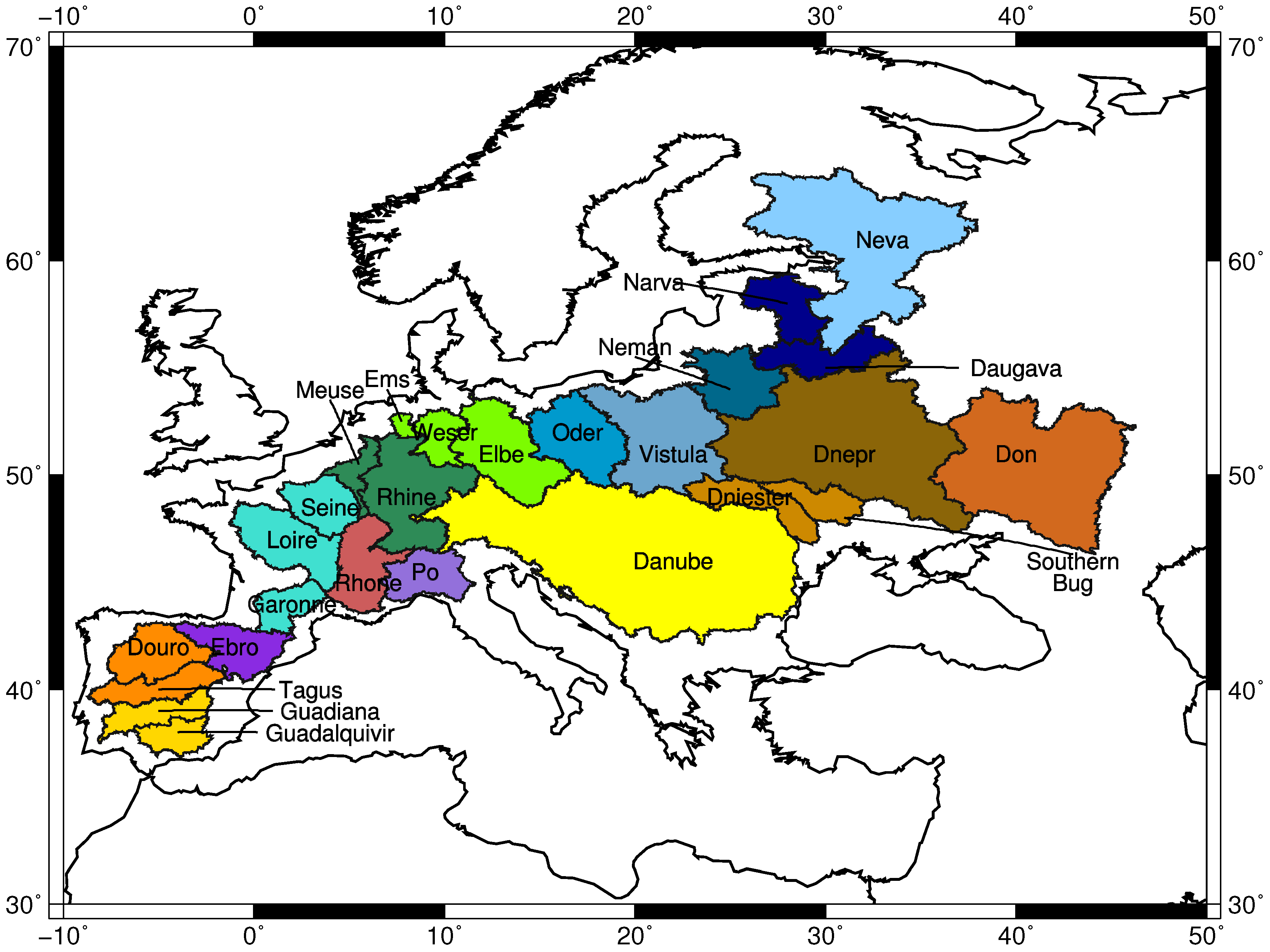
Twenty-six major European river basins were considered in this study (Figure 1). The border of each basin is defined by the catchment associated with the most downstream gauging station. Small neighboring catchments are merged together for water budget analyses taking into account the main European watersheds (marked by colors in Figure 1). This is necessary because of the limited spatial resolution of GRACE-derived TWS. The 17 combined catchments are listed in Table 1 together with their size ranging from ~70,000 km for the Po to ~800,000 km for the Danube.
2.2. GRACE
The twin satellite mission GRACE (Gravity Field and Climate Experiment [26]) has been measuring spatial and temporal variations of the Earth’s gravity field since 2002. GRACE consists of two satellites following each other on the same orbit. An inter-satellite K-band microwave link observes orbit variations caused by an inhomogeneous mass distribution on Earth. Temporal variations in gravity can then be converted to mass changes in terms of equivalent water height according to [27] taking into account the elastic loading effect.
In this study, we use GRACE release 05 (RL05) time series [28] provided by the German Research Center of Geosciences (GeoForschungsZentrum, GFZ). The monthly GRACE solutions were smoothed using a DDK4 filter [29] to account for the typical anisotropic error striping patterns. To consider the effect of seasonal and secular geo-center variations, we added the degree-one spherical harmonic coefficients provided by [30,31] to the GRACE solutions. The C20 coefficient, which cannot be well determined by GRACE, was replaced by a result obtained from satellite laser ranging [32]. Already during the GRACE processing chain, temporal gravity field variations caused by tides (ocean, Earth and pole tides), as well as by atmospheric and non-tidal ocean mass variations were subtracted from the observations prior to the gravity field estimation step. Additionally, the mass trend caused by glacial isostatic adjustment (GIA) [33] was removed in post-processing. Therefore, the resulting mass variations primarily reflect hydrological water storage changes. For a realistic estimation of the GRACE measurement accuracy, we used the calibrated errors provided by GFZ, as well as the standard deviations provided together with the degree-one and of the C20 coefficients in our variance propagation procedure (see Section 3.4).
2.3. Numerical Weather Prediction Models
2.3.1. COSMO-REA6
COSMO-REA6 is among the first reanalysis results covering only a part of the globe, but at a much larger spatial and temporal resolution than all available global reanalyses (see the next subsections). Other regional reanalyses are the North American Regional Reanalysis (NARR) [34], the arctic system reanalysis [35], or the recent European reanalyses from the U.K. MetOffice [36], or the Swedish Meteorological and Hydrological Institute (SMHI) [37].
The general goal of these regional reanalyses is to provide a physically consistent and homogeneous climate dataset of the atmosphere and land surface that resolves atmospheric patterns on spatial scales from 500 km down to about 10 km (also known as atmospheric mesoscale). Important weather and climate phenomena are situated in the mesoscale range e.g., frontal passages, land sea circulations or deep convection events. Furthermore, the effects of orography and land sea distribution (especially with respect to precipitation) are expected to be much better represented than in models with grid sizes of 50–100 km, which are common in global models due to the computational burden. Global reanalyses still play an important role because they provide the atmospheric boundary conditions to the regional high-resolution models.
The COSMO-REA6 uses the regional assimilation and forecasting system of the German National Meteorological Service (Deutscher Wetterdienst, DWD) [38]. It combines the non-hydrostatic forecast model COSMO with the continuous data assimilation method nudging [39]. The region covered by COSMO-REA6 is identical to the European Coordinated Regional Climate Downscaling Experiment at 0.11 resolution (CORDEX-EU11) domain, but with a grid size of 0.055 (~6 km), on a rotated latitude-longitude grid with 40 vertical layers in the atmosphere, between the surface and about a 20-km height. Prognostic variables are the three-component wind velocity vector, temperature, pressure and various water substance concentrations to account for the generation of clouds and precipitation in liquid and solid phases. Observations come from different observing systems like radiosondes, air planes, vertically pointing wind profilers, surface stations, buoys and ships. Depending on the observing system and the observed variable, windows of influence are defined that spread the actual observations to the neighboring grid cells in space and time. Nudging means that each equation for the prognostic variables temperature, pressure, wind velocity and moisture concentration is supplemented by an additional forcing term. This forcing term drives the model solution at any time and at all grid points to the respectively spread observations using a prescribed time scale. Note that this procedure will provide consistent prognostic variables through their physical connection dictated by the equations, but it cannot provide consistent budgets of energy and water because the additional forcing terms always add energy, water and momentum to the system proportional to the difference between the simulated and the observed values. Fluxes like precipitation and evapotranspiration are derived internally from the necessary state variables, but are in general not assimilated. Therefore, an evaluation of precipitation, evapotranspiration and other energy or water fluxes with independent data as is presented here is an important contribution to the overall quality assessment of the COSMO-REA6 or any other regional reanalysis.
The actual setup of COSMO-REA6, including the necessary preparation of land surface variables, like soil moisture, and oceanic variables, like sea surface temperatures, can be found in [9]. Here also, a first quality assessment of COSMO-REA6 is presented. Precipitation as one of the most interesting climate variables is further evaluated in [40], where also a comparison over Germany of the global reanalysis ERA-Interim, the U.K. Met Office and SMHI European reanalyses and an even higher resolution COSMO reanalysis at a 2-km grid size is presented, showing among other features the importance of resolution in representing precipitation.
2.3.2. ERA-Interim
The global Interim ECMWF Reanalysis (ERA-Interim) provides gridded fields of atmospheric and land surface variables with approximately 79-km grid spacing considering 60 vertical levels. The model output covers the time span from 1979 onwards at three-hourly resolution. The main objectives of the ERA-Interim reanalysis are a realistic representation of the hydrological cycle and temporal consistency in order to estimate reliable trends [16]. The sequential data assimilation system is based on the 4D-Var method [41]. In a 12-hourly cycle, the current state of the atmosphere is estimated from a forecast model combined with an important number of observations originating in the majority from satellites.
In this study, synoptic monthly means of precipitation and latent heat flux are evaluated, which are computed by the model from temperature, humidity, wind speed and radiometer observations. Compared to [8], here, we use a finer grid of 0.75 × 0.75.
2.3.3. MERRA-2
While in [8], we assessed the performance of the Modern-Era Retrospective analysis for Research and Applications (MERRA) model, here we moved on to its successor MERRA-2. For data assimilation, an incremental analysis update scheme is applied by the Goddard Earth Observing System Version 5 (GEOS-5). MERRA-2 assimilates new observation types such as hyperspectral radiance, microwave, GPS radio occultation, ozone and aerosol datasets [17]. One particular improvement of MERRA-2 is the correction of precipitation biases using observation-based precipitation from different sources [42,43]. However, in this study, we assess the uncorrected precipitation in order to compare with the other two reanalyses.
MERRA-2 is provided by the Goddard Earth Sciences Data and Information Service Center (DISC) from 1980 onwards with one-hourly temporal resolution on a 0.625 × 0.5 grid. Here, monthly outputs of modeled precipitation and surface latent heat flux are assessed.
2.4. Observational Datasets
In this study, the ability of P and E from NWP models to close the water budget equation is compared to the performance observation-based datasets, i.e., the Global Precipitation Climatology Centre (GPCC) dataset for P and the Global Land Evaporation Amsterdam Model (GLEAM) for E.
2.4.1. GPCC
We used the recent version of the GPCC Full Data Reanalysis (V7) that covers the period 1901–2013 and is available at 0.5 resolution from the GPCC web site [18]. The precipitation dataset is based on 75,000 gauging stations world-wide, which are subject to strict quality control. The monthly product is optimized for water budget studies [44]. GPCC data were also used as a reference by [9] for assessing the quality of P generated by COSMO-REA6.
2.4.2. GLEAM
GLEAM estimates the individual components of evapotranspiration using satellite observations together with model data and a set of algorithms [19,20]. First, the Priestley and Taylor equation [45] is used to calculate potential evaporation from net radiation and air temperature observations. Then, actual evaporation is derived by applying a multiplicative stress factor based on microwave vegetation optical depth and soil moisture observations. Three datasets exist with different forcings and spatio-temporal coverages. Of these, two datasets of limited geographical extent are exclusively based on satellite data. Here, we use the only global dataset, GLEAM_v3.0a. For GLEAM_v3.0a, net radiation and air temperature are obtained from ERA-Interim, but all other required input datasets (precipitation, soil moisture, vegetation optical depth, snow water equivalent) are observation based. GLEAM_v3.0a has a spatial resolution of 0.25 and is a daily dataset, which spans the period 1980–2014.
In [8], we used a gridded E dataset based on the current global network of eddy covariance towers (FLUXNET) provided by the Max Planck Institute (MPI) Jena. The MPI dataset is available only until 2011 and was therefore replaced by GLEAM. However, the authors of [20] found good agreement of GLEAM and FLUXNET data.
2.5. Discharge
Monthly discharge data from the Global Runoff Data Centre (GRDC) are available for limited periods of time only (Figure 2). Merely 10 out of 26 stations used in this study provide data covering parts of the GRACE time span. Approaches for extending discharge data in time became ever more relevant during the last few years [46], e.g., satellite altimetry, runoff-precipitation ratio and runoff-storage relationships. Here, we created a consistent discharge time series by calibrating the lumped rainfall-runoff model GR2M [25]. GR2M (a) is a simple empirical monthly model, (b) achieves good results for river basins of different sizes and with different hydrological conditions [47] and (c) allows for easy inclusion of error estimation. Further model improvement was achieved by extending GR2M using a distributed Hydrologiska Byrans Vattenavdelning (HBV) type snow model.
For each of the 26 river basins, the GR2M-snow model was calibrated against GRDC data using the 10 most recent continuous years available (marked in light blue in Figure 2). Then, the model was run for the GRACE time span. In addition, error estimates were obtained by running GR2M-snow several times with disturbed forcings and disturbed parameters. Finally, discharge from GR2M-snow was merged for the 17 aggregated catchments including error propagation. The resulting discharge time series were used in the further course of this study. While time series of P, E and are averaged over each basin, discharge is available at the most downstream gauging station, which also defines the border of the catchment.
3. Methodology
Water storage changes and discharge R are linked to net atmospheric-terrestrial flux via the water budget equation:
Consistent time series of water flux and storage are required for assessing the closure of the water budget equation. In this section, we first describe the derivation of the time series of and . Afterwards, the set up of the rainfall-runoff model GR2M is presented aiming at the computation of discharge time series R covering the whole GRACE period. Finally, evaluation measures and the error assessment strategy are described.
3.1. Consistent Time Series of Atmospheric-Terrestrial Flux and Storage Change
First, GRACE-derived gridded total water storage (TWS) anomalies S were centered to the 11-year study period by removing the mean static field computed from 2003–2013. Next, monthly time series of P, E and S were computed by spatially averaging over all grid cells of the target area. Finally, storage changes were obtained for each month as central differences from the GRACE storage time series according to:
where is the previous month and the next month. Central differences in contrast to backward or forward difference operators avoid introducing a phase shift in the TWS change time series. Spatial averaging of TWS involves attenuation of the signal due to the spectral characteristics of GRACE data and further distortion due to the filtering procedure, known as the leakage effect [48]. Depending on the mass distribution, filter properties, and target area, mass is transported either into the basin (leakage in) or out of the basin (leakage-out). This effect becomes particularly large if the basin is very small or if the mass distribution outside and inside of the basin differs significantly [49]. Consequently, GRACE-derived time series of TWS change need to be rescaled. To this end, time-variable rescaling factors were derived for each target area separately. Assuming that the spatial distribution of approximately corresponds to the spatial distribution of , a number of different P and E datasets were used to simulate the effects from spectral resolution, filtering and leakage. A robust estimate for the multiplicative rescaling factor of each month was obtained from the median of the analyzed datasets. More detailed information on the derivation of consistent time series are provided by [8].
3.2. Using GR2M-Snow for Generating Modeled Discharge Time Series
The 2-parameter rainfall-runoff model GR2M requires as input monthly precipitation and potential evapotranspiration and includes two stores, a production store of variable size and a routing store with a fixed capacity of 60 mm. Monthly discharge is simulated by calibrating the capacity of the production store and an exchange coefficient, which accounts for the exchange of water with the outside of the basin. GR2M was extended by a distributed HBV-type snow model, which requires gridded temperature as input and adds three more calibration parameters (melting temperature, melting coefficient and temperature separating rain and snow). If the temperature is smaller than a defined value, snow is added to the corresponding grid cell, and if the temperature exceeds the melting temperature, the melting coefficient defines the amount of snow that is subtracted from the grid cell. Then, snow loss is accumulated over all grid cells and considered as additional precipitation. The precipitation and temperature datasets were obtained from the European daily high-resolution gridded dataset (E-OBS [50]) and potential evapotranspiration from the Climate Research Unit (CRU) data set TS3.22 [51]).
GR2M-snow was calibrated for each of the basins against observed discharge for the 10 most recent continuous years available from GRDC (Figure 2) minimizing the squared difference of observed and simulated discharge. As GRDC data are erroneous for Neman and Vistula watersheds, those basins were calibrated against data from E-RUN (observational gridded runoff estimates for Europe) [52]. Then, the model was run for the time span 1950–2013. As the validation period for each basin, the next 10 years available before the calibration period were chosen. In addition, error estimates were derived by generating an ensemble of simulated discharge by disturbing both the parameters and the input datasets. The input datasets were disturbed with noise following a Gaussian distribution, applying a standard deviation of 1 C for temperature, 20% for precipitation and 5% for potential evapotranspiration. The variabilities of the five calibration parameters follow uniform distributions with appropriate uncertainty assumptions chosen for each parameter individually. For each river basin, 1000 model runs were performed, and from the ensemble of modeled discharge time series, the standard deviation was computed. The resulting error band fits well to the difference between GRDC and GR2M-snow (see Section 4.1). Furthermore, we were able to reproduce the results from [8] using discharge simulated by GR2M-snow within the error estimates. However, we are aware of limitations of this approach, e.g., when river dynamics changed over time due to river management and/or construction.
The skill of GR2M-snow in simulating discharge is evaluated by assessing different measures for the validation period, i.e., the mean bias and the root mean squared error (RMSE) between observed and simulated discharge, and Nash–Sutcliffe (NS) coefficients [53] for the time series with seasonal cycle and for de-trended and de-seasoned time series. NS coefficients are computed according to:
where is observed discharge from GRDC, the temporal mean of observed discharge and simulated discharge from GR2M-snow. Here, NS coefficients are computed from the root of discharge in order to avoid too much weight on high discharge values. An NS coefficient of one means perfect agreement between observed and modeled discharge; values between zero and one imply that the model better simulates discharge than the mean of observed discharge. In the case of NS coefficients smaller than zero, the mean of observed discharge better represents actual discharge than the model.
3.3. Evaluation of the Water Budget Equation
The performance of the individual datasets is assessed with respect to using the following measures computed for the whole study period (2003–2013). A four-parameter model was fitted to the time series of basin averages for both sides of the water budget equation:
where T is the annual period and the residuals. A difference between the mean a of the time series of and is defined as the bias of atmospheric-terrestrial flux. Parameter b corresponds to the trend, and amplitude and phase shift are derived from c and d. Additionally, correlations of the time series and of de-seasoned and de-trended time series were investigated.
3.4. Error Assessment
For assessing the significance of our results, we performed a thorough error assessment for . Calibrated errors given for monthly GRACE Stokes coefficients were propagated to the basin-averaged TWS changes while taking into account errors from degree-1 and -2 coefficients. However, the resulting error estimates might be too optimistic, as we neglect errors from the GIA model and from the rescaling procedure. The uncertainty of simulated discharge was obtained from ensemble runs with the GR2M-snow model by disturbing model parameters and input datasets. Then, errors were propagated further to for each of the aggregated catchments.
4. Results
Overall, the results presented below show the skill of the individual datasets in closing the water budget equation over Europe. First, the individual components of the water budget equation are analyzed. Then, both sides of the water budget equation are contrasted for selected target areas. Finally, biases, amplitudes and trends are illustrated and discussed for the whole study area.
4.1. Modeled Discharge from GR2M-Snow
Discharge simulated from GR2M-snow generally fits well to available discharge from GRDC within the error bounds. Figure 3 shows discharge for the Rhine basin from GRDC (blue) and GR2M-snow (red). Only a few peaks from GRDC exceed the ensemble-based standard deviation (grey).
The influence of discharge on the closure of the water budget equation depends not only on its magnitude, but also on the magnitude of TWS change. The magnitude of discharge and its standard deviation vary for the individual river basins with temporal means between 3 and 61 mm/month (Table 2). The largest values are found in central Europe where mean discharge rates are larger than 40 mm/month and corresponding standard deviations larger than 7 mm/month (Rhine, Rhone and Po). In contrast, many basins in eastern Europe, in France and on the Iberian peninsula have mean discharge rates of about 10–20 mm/month and standard deviations of only 2–5 mm/month. In general, the standard deviation derived from ensemble runs amounts to 20%–30% of simulated mean monthly discharge (Table 2). An exception is the Daugava, where the standard deviation is about 40% of simulated discharge. Root mean squared errors (RMSE) between observed and simulated discharge have in most basins approximately the size of the simulated standard deviations.
The bias of mean discharge for the validation period is smaller than 2 mm/month (Table 2) except for Po (4.0 mm/month) and Rhone (2.5 mm/month), and thus, we neglect its contribution to the closure of the water budget equation. Nash–Sutcliffe coefficients (NS) were computed for the validation phase and confirm that the calibration of GR2M-snow was successful for most basins. In western and central Europe, the NS coefficients reach values between 0.6 and 0.9. Only some basins in eastern Europe (Narva, Dnepr, Southern Bug and Don) have NS coefficients smaller than 0.3. Discharge from Don contains some extreme peaks during the validation time span that are not simulated by GR2M-snow, resulting in a negative NS coefficient. NS coefficients for de-seasoned and de-trended time series (computed according to Equation (4), extended by semiannual signals) are mostly between 0.2 and 0.6. Again, the largest values are obtained for western and central Europe with NS coefficients between 0.35 and 0.65. Negative NS coefficients of de-seasoned and de-trended time series are found for Danube, Don, Neva and Po indicating changes in the short-term behavior of discharge between the calibration and the validation time span. However, correlations are between 0.8 and 0.9 for the original time series and between 0.7 and 0.8 for de-seasoned and de-trended time series. Exceptions are the rivers Don and Neva, where correlations of de-seasoned and de-trended time series amount only to 0.3 and 0.4.
4.2. Time Series of Fluxes and Storage Change
The noise of depends mainly on the size and the shape of the target areas [49]. For example, the Danube has a smooth time series with standard deviations of about 10 mm/month, while the time series of the Po is very noisy, and the standard deviations reach up to 30 mm/month, which is half of the annual amplitude (Figure 4). In fact, with a size of only 70,000 km, the Po basin is likely too small for obtaining reliable TWS information from GRACE.
In the following, time series of fluxes for five catchments from different regions in Europe and of different sizes are discussed in more detail: (a) Guadiana-Guadalquivir on the Iberian peninsula, which is a small region and the most southern target area with very dry climatic conditions, (b) Rhine-Meuse in central Europe with a medium size and large precipitation events in the Alpine region, (c) Neva, the most northern basin, (d) Dnepr, a catchment with particularly low precipitation rates, and (e) Danube, the largest river basin in Europe. Some, but not all findings from these regions can be transferred to basins with similar climatic conditions (see Section 4.3).
The magnitude of river discharge varies in the individual basins depending on the climatic conditions (Figure 5, black dashed line). In Guadiana-Guadalquivir and Dnepr, discharge is small with mean annual values of 7–9 mm/month and 0–14 mm/month. In contrast, discharge plays an important role in central Europe (Rhine-Meuse) where it amounts to mean annual values of 30 mm/month, which is one third of precipitation. While discharge in the Neva basin is relatively constant with a weak annual cycle, in the Rhine-Meuse and Danube basins, it is clearly related to individual precipitation events. For most basins, discharge contributes about 10%–20% to the error of the left-hand side of the water budget equation. The highest error contribution from discharge is found in the Danube basin with 40%, which is mainly due to the small standard deviation of GRACE data caused by the large basin size.
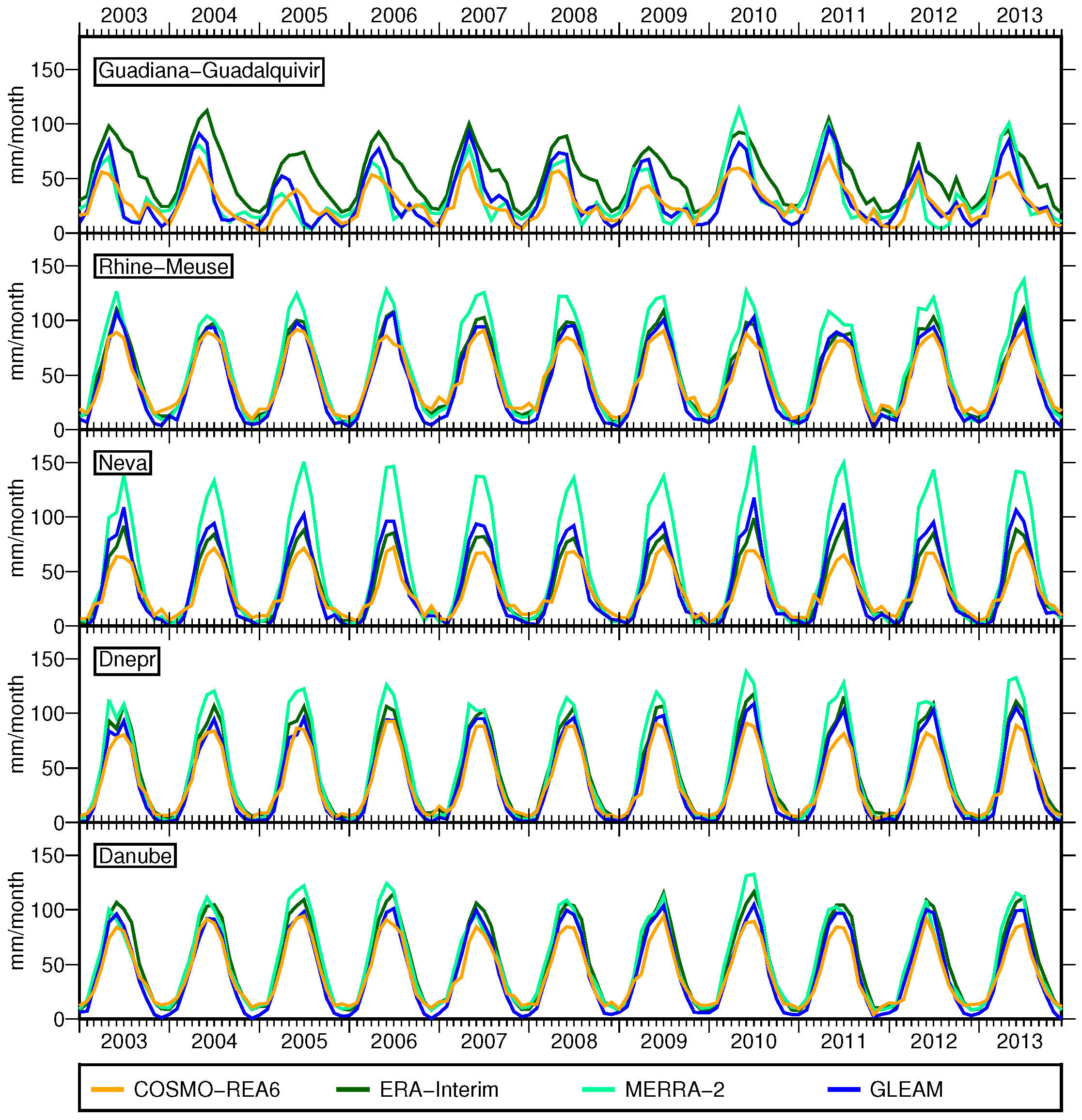
Monthly total precipitation is highly variable for European river basins (Figure 5). The chosen catchments represent different climatic conditions over Europe, e.g., there is nearly no precipitation in summer in Guadiana-Guadalquivir; Neva has a very pronounced annual cycle; and in Rhine-Meuse, individual precipitation events are visible. All model-derived time series show similar features as the observation-based dataset GPCC. However, while in the Danube basin, peaks from all models have about the same size, we find in the Dnepr and Neva basins smaller peaks for the COSMO-REA6 model compared to the other datasets. The authors of [54] showed that COSMO-REA6 has an enhanced skill in representing individual precipitation events compared to ERA-Interim. Moreover, the authors of [9] found that COSMO-REA6 and ERA-Interim overestimate P over parts of Russia and parts of the Alps compared to GPCC. In our study, this is confirmed by particularly high P rates in the Rhone basin for COSMO-REA6 with a temporal mean of 90 mm/month and peaks of up to 180 mm/month. Furthermore, in line with [9], we found that all reanalyses underestimate P in the catchment of Garonne-Loire-Seine compared to GPCC. Besides, MERRA-2 simulates exceptional high P rates in the Neva basin where its temporal mean is more than 10 mm/month higher than the temporal mean from the other datasets.
Evapotranspiration is characterized by a distinct annual cycle over Europe with different amplitudes depending on the regional climate (Figure 6). Large differences are found between the individual E datasets with a mean spread of 17 mm/month (maximum 43 mm/month) in the Danube basin, up to a mean spread of 28 mm/month (maximum 96 mm/month) in the Neva basin, and a mean spread of 29 mm/month (maximum 68 mm/month) in the catchment of Guadiana-Guadalquivir. Interestingly, E for the catchments on the Iberian peninsula does not only show a large spread between the models, but also patterns beyond the annual cycle. Moreover, all models except ERA-Interim suggest a small, but not regularly occurring secondary peak of evapotranspiration in winter in Guadiana-Guadalquivir. One might speculate that this sub-annual variability is due to the interaction of large-scale variability with regional characteristics, e.g., effects of the North Atlantic Oscillation (NAO). In summer, evapotranspiration from ERA-Interim is twice as large as E from COSMO-REA6 in Guadiana-Guadalquivir. Furthermore, in the Guadiana-Guadalquivir basin, MERRA-2 fits best to the observation based dataset GLEAM.
In general, MERRA-2 overestimates E compared to the observation-based dataset GLEAM with the most extreme values in the Neva catchment, where the temporal mean is 20 mm/month higher than the temporal mean from the other models. In contrast, outputs from COSMO-REA6 show the smallest E in all considered basins. It is striking that for most basins, the maximum value in summer is quite the same for COSMO every year, whereas for the global models, it varies from year to year. The year 2010 stands out with high evapotranspiration values for some models, which could be explained by the heat waves over Russia and the Iberian peninsula.
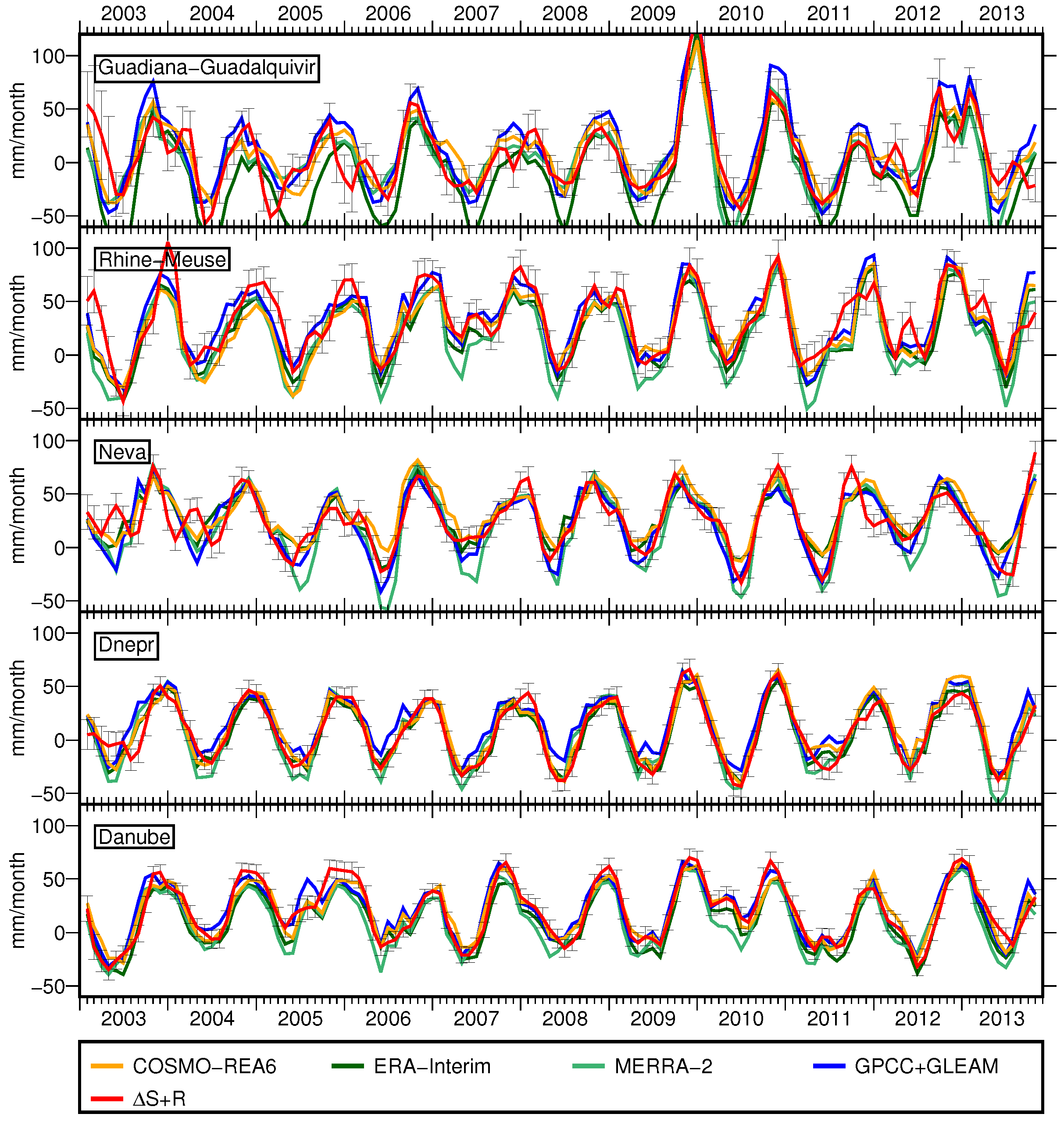
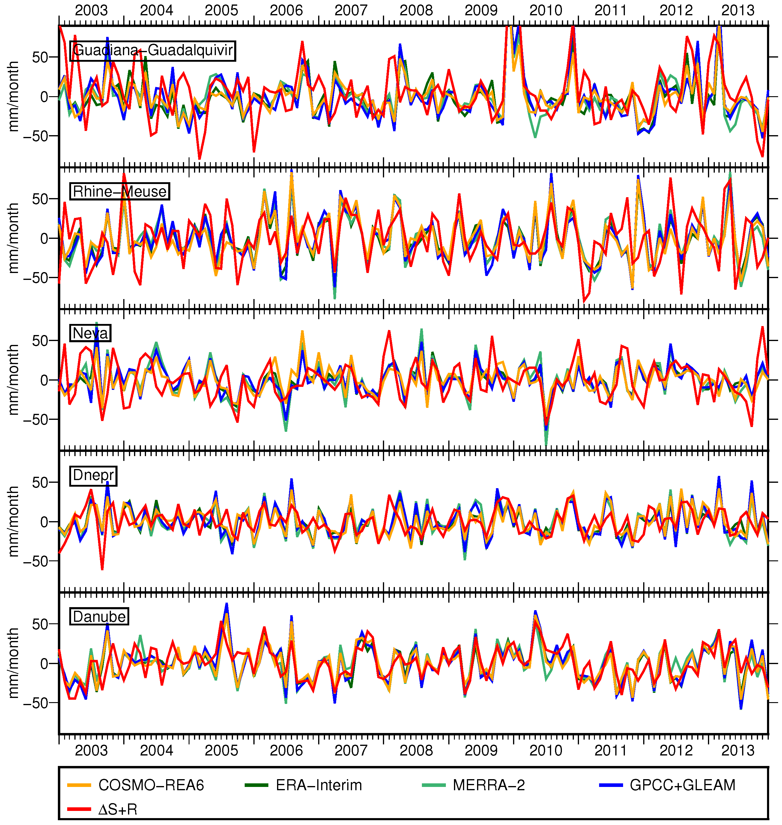
The previous analyses already indicated that the performance of the models shows regional differences. This also impacts the closure of the water budget equation (Figure 7 and Figure 8). Modeled is mostly within the error bars of even in smaller basins (Figure 7). However, MERRA-2 tends to underestimate especially in summer due to large E estimates. Furthermore, ERA-Interim cannot close the water budget equation on the Iberian peninsula as E is overestimated in this region. It is worth noticing that from COSMO-REA6 matches well for all selected catchments. The other models mainly differ from by a constant shift. Correlations between and are between 0.5 and 0.9 and mostly about 0.7 for all models (Figure 9a), which is mainly attributed to the annual cycle.
A closer look at short-term variability is taken in Figure 8. For this purpose the mean, trend and annual signals according to Equation (4) (extended by semiannual signals) were subtracted from the flux time series. De-seasoned and de-trended time series show similar patterns for both sides of the water budget equation in all basins. Short-term variability also depends on the climatic conditions of the target catchment, e.g., in the Dnepr basin de-trended and de-seasoned and have maximum values of 50 mm/month, whereas in Guadiana-Guadalquivir catchment, maximum values of 100 mm/month exist.
Best agreement between de-trended and de-seasoned and is achieved for the Danube with correlations of about 0.7 (Figure 9b). In most basins, the correlation is about 0.5, with a few exceptions like the Ebro, Neman, Don and Neva, where correlation is smaller than 0.3. Especially in smaller basins, outliers in the GRACE time series have a huge impact on correlation. Furthermore, in some basins, the agreement between and changes with time, e.g., in the Guadiana-Guadalquivir and Neva basins, models and disagree during the first three years of the study period, but then again match very well (Figure 8).
4.3. Statistics of the River Basins
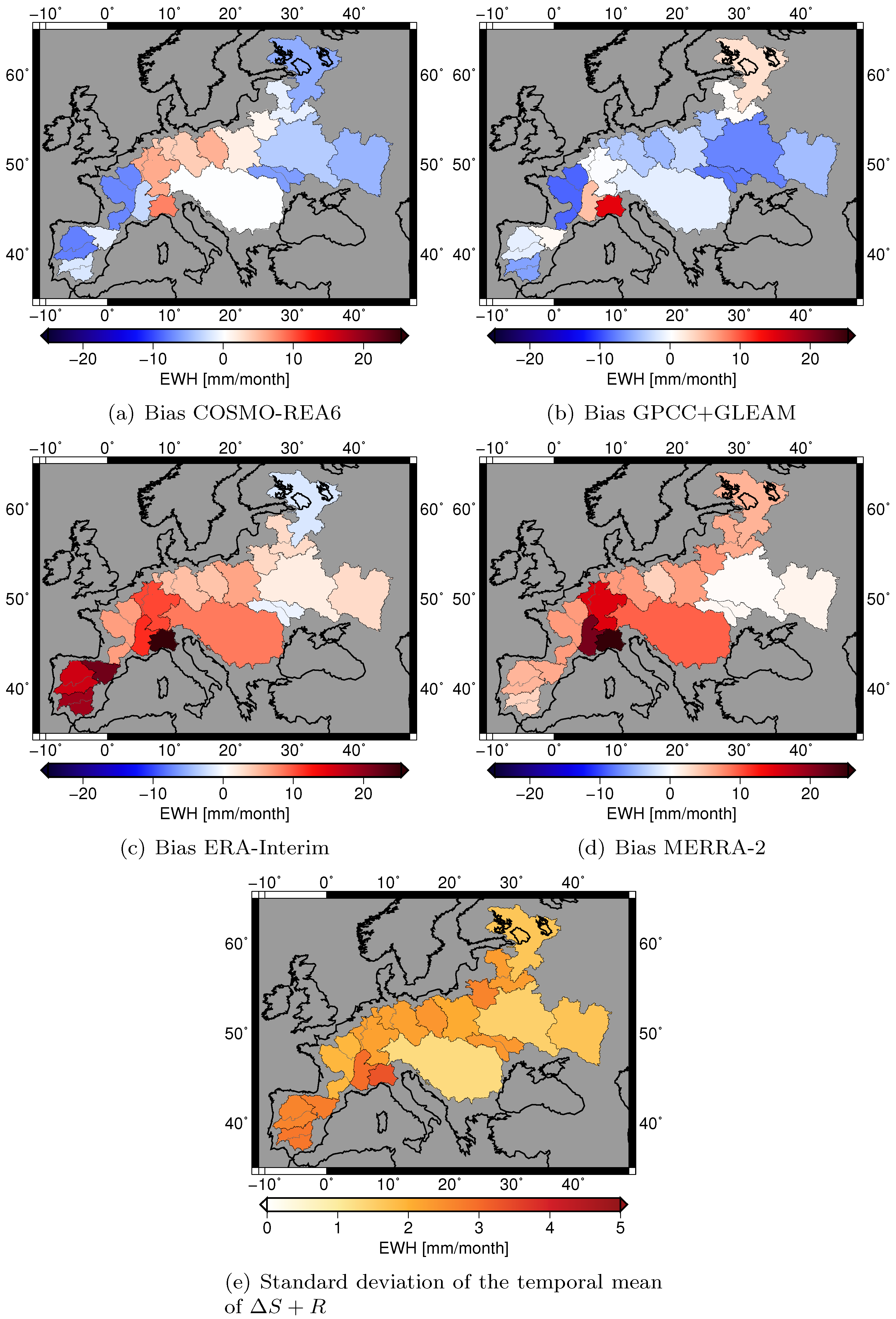
After integration, biases in fluxes produce incorrect trends in storage, i.e., underestimating leads to a negative trend in storage, and overestimating leads to a positive trend in storage. Figure 10a–d shows the bias of the water budget equation for the individual datasets. The global models ERA-Interim and MERRA-2 tend to underestimate (indicated by the red color). For ERA-Interim, the largest biases (about 20 mm/month) are obtained on the Iberian peninsula, which we attribute to deficiencies in the E estimate as discussed before. In contrast, in eastern Europe, both global models perform quite well with biases smaller than 10 mm/month. Although MERRA-2 shows the largest biases in central Europe (15 mm/month for Rhine-Meuse), it improved with respect to MERRA, which was assessed in [8], and had biases of about 25 mm/month in some central European basins. Results for the basins of Po and Rhone should be interpreted with caution as the basins are too small for deriving reasonable storage changes from GRACE data, and moreover, simulated runoff is rather uncertain in these basins (Table 2).
Biases of COSMO-REA6 are smaller than 10 mm/month in all basins, and in many basins, even smaller than 5 mm/month. In central Europe, COSMO-REA6 tends to underestimate , whereas in eastern and western Europe, it overestimates . The relevance of the bias is illustrated by Figure 10e, which provides the standard deviation of the temporal mean of . This value is mostly between 2 mm/month and 3 mm/month; it is smaller for large basins like Danube and Dnepr and higher for the very small basins like Po, Rhone and Ebro. We can conclude that the biases found in COSMO-REA6 are relevant only for a few basins. The observation-based datasets GPCC and GLEAM also tend to overestimate with large values in the catchments of Garonne-Loire-Seine (−9 mm/month), Dnepr (−7 mm/month) and Dniester-Southern Bug (−8 mm/month). Interestingly, no obvious biases are found in the eastern basins for all model-based time series of .
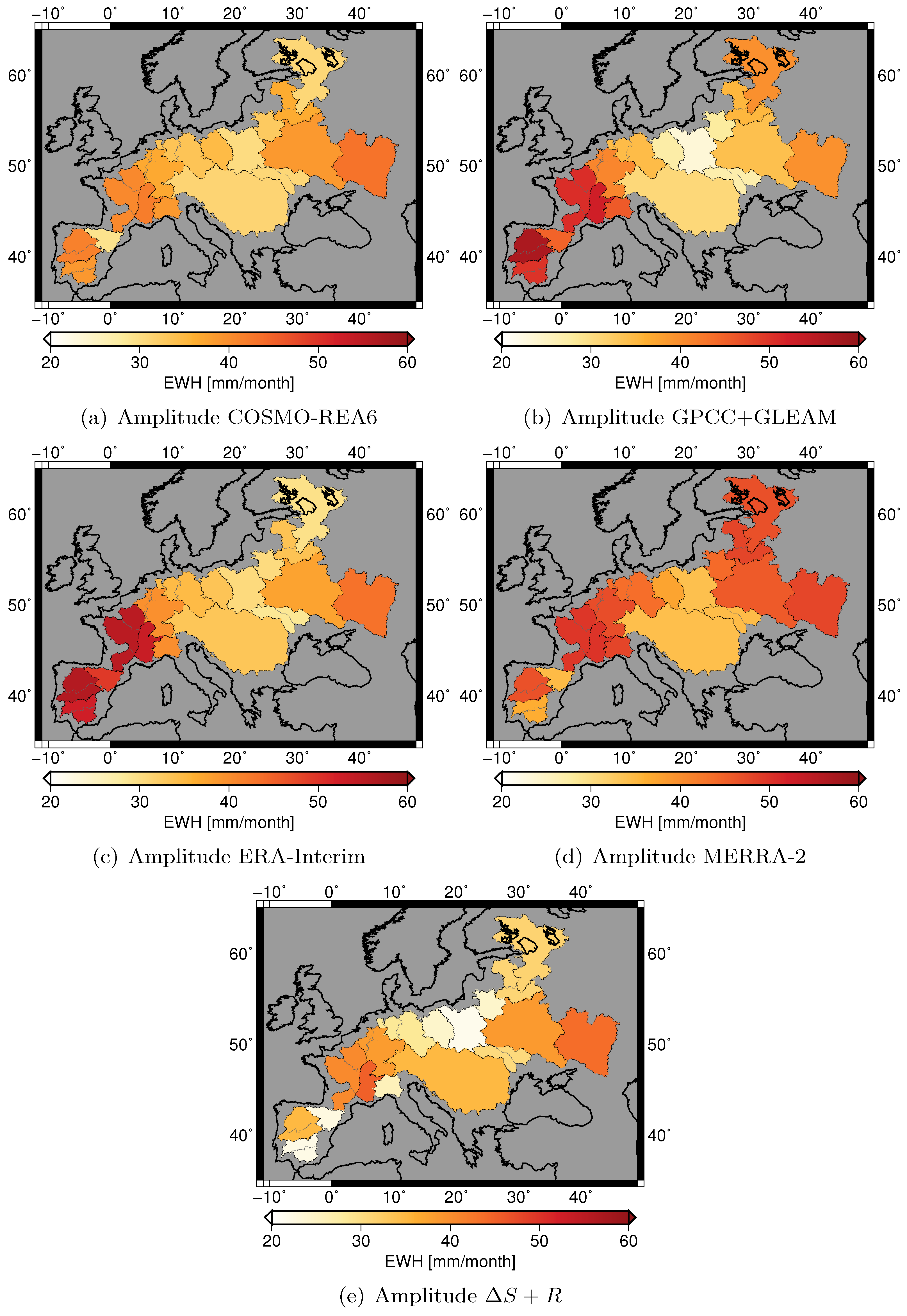
A more complete picture of the closure of the water budget is obtained by analyzing the amplitude, phase and trend of and derived from the parameters estimated from Equation (4). The amplitude of is predominantly affected by modeled evapotranspiration, which differs largely for the individual models (Figure 6). The regional patterns and the magnitudes of the amplitudes of COSMO-REA6 fit well to the amplitudes of with exceptions only in a few basins, e.g., on the Iberian peninsula (Figure 11). In contrast, GPCC in combination with GLEAM and ERA-Interim overestimate the amplitude of with respect to GRACE by 15–20 mm/month in all basins west of the Rhine. The amplitude of from MERRA-2 is particularly large in the French basins, the Rhine and the eastern basins with values of about 50 mm/month. The Danube basin stands out as all time series and also agree very well regarding the amplitude with values between 31 and 35 mm/month. While COSMO-REA6 and ERA-Interim have nearly no phase shift, MERRA-2 and GPCC+GLEAM are contaminated with phase shifts of up to 10 days.
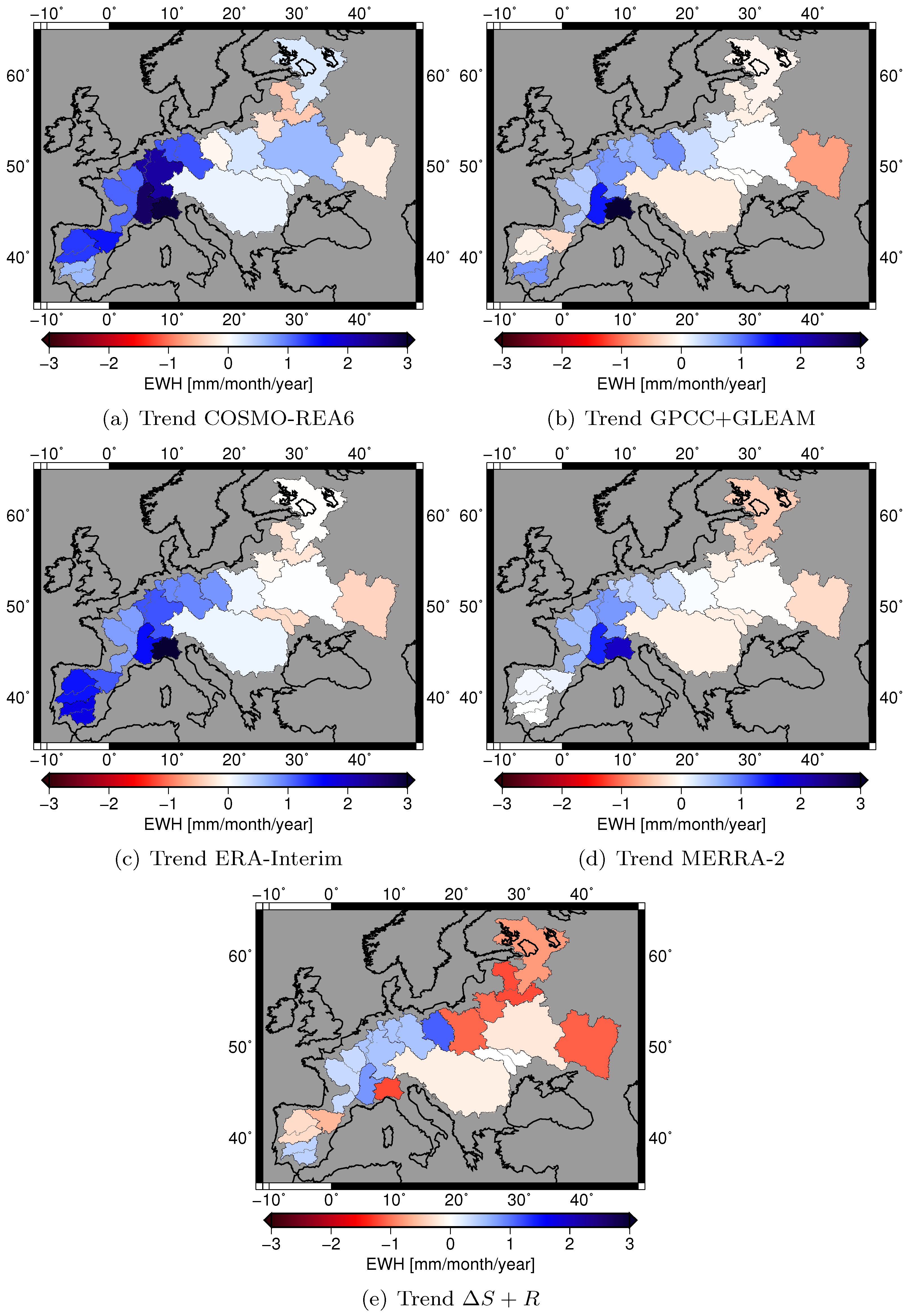
Negative trends in fluxes imply increasingly fast drying; positive trends mean that a region experiences increasingly fast wetting. Within the time span considered here, all models agree that eastern Europe tends to become more and more dry and central and northwestern Europe more and more wet (Figure 12). This conclusion is confirmed by ; however, GRACE and discharge time series indicate larger negative trends in eastern Europe than the models. The authors of [55] found similar trend patterns investigating runoff over Europe, with negative trends over eastern Europe and positive trends over northwestern Europe for the time period 1963–2000. In contrast, the authors of [3] found negative trends for changes of between 1976–2005 and 2070–2099 in our whole study region. The authors of [56] compared P and E for the time periods 1948–1968 and 1985–2005 and identified drying trends over parts of eastern Europe and the Iberian peninsula, but no sign of wetting trends over northwestern Europe. The largest positive trends in northwestern Europe are found by COSMO-REA6 with 1–3 mm/month/year. Over the Iberian peninsula, the results are unclear. While ERA-Interim and COSMO-REA6, reanalyses show positive trends of on the Iberian peninsula; GPCC + GLEAM and identify positive trends only in the southern catchment Guadiana-Guadalquivir and negative trends in the northern part of the peninsula; and MERRA-2 indicates no trend at all.
5. Discussion and Outlook
Our results suggest that the high resolution COSMO-REA6 reanalysis better closes the water budget equation than global reanalyses. This means COSMO-REA6 can be seen as an important step forward in the consistent representation of the water cycle over Europe and, thus, advances climate monitoring on regional scales. In fact, in comparison to global NWP models, COSMO-REA6 improved the representation of small-scale variability, especially with respect to the accuracy of precipitation events [9].
We investigated the closure of the water budget equation for all major European river basins, aggregated to 17 catchment areas. This allowed us to distinguish regional patterns for the performance of the individual models over Europe. Previously, most water budget studies focused on large river basins worldwide (e.g., [14,57,58]). Only a few studies investigated the closure of the water budget over different river basins in Europe [8,10]. However, [10] assessed moisture flux convergence instead of . Due to the limited resolution of the early GRACE releases, they found very poor agreement between GRACE and ECMWF data. In [8], we focused on only four catchment areas in central Europe, which were too few for determining regional patterns. We summarize that the current study provides unique insights into the performance of different datasets over Europe due to (i) the extension of the study area, (ii) the long study period of 11 years and (iii) the usage of the latest GRACE release.
Discharge was modeled applying a simple calibrated rainfall-runoff model instead of using gauge observations like in most water budget studies (e.g., [8,14]). In doing so, we circumvented the problem of lacking recent discharge data; yet, this approach may have limitations, and further research is required. Modeling introduces additional uncertainty to the left-hand side of the water budget equation, which was taken into account by modeling the error of simulated discharge via ensemble runs. We obtained errors of 20–30% of the magnitude of discharge, which we believe is a rather conservative estimate. Furthermore, the NS coefficients indicate a successful calibration of the model in most river basins. However, it should be kept in mind that the computed errors do not take into account changes due to human activities (e.g., dams, redirection) between the calibration time span and the GRACE time span. Nevertheless, the largest contribution to the error of (about 60–80%) originates from GRACE as discharge is much smaller in most basins. Especially in the very small river basins (e.g., Rhone, Po), the GRACE data should be interpreted with caution due to their excessive noise on such small spatial scales.
For most catchments, modeled from COSMO-REA6 lies within the error ranges derived for . Biases are mostly smaller than 5 mm/month. In contrast, ERA-Interim and MERRA-2 underestimate with particularly large biases over the Iberian peninsula for ERA-Interim and over Rhine-Meuse for MERRA-2. This confirms the results obtained in [8] for central Europe. However, it is worth noticing that the bias of MERRA-2 became smaller compared to the bias obtained for MERRA in [8]. We attribute this to changes in the data assimilation system. For hydrological studies and climate modeling, it is particularly important to reduce the bias of in order to avoid introducing unrealistic trends in storage.
Evapotranspiration was found to be the most uncertain component of the water budget equation over Europe. In accordance with [14], who compared E from various models to GRACE-based estimates and detected significant differences in the mean annual cycles, we found differences in the annual amplitude of up to 50 mm/month between the individual E datasets. In particular, on the Iberian peninsula and for the northeastern catchments, large uncertainties for E were determined. It is likely that the spread of the models on the Iberian peninsula arises from the differences of potential evaporation and actual evaporation in this region.
The annual amplitude of is mainly affected by the annual cycle of E. Compared to , the global datasets overestimate the annual amplitude especially in western Europe. In contrast to this, the amplitude of COSMO-REA6 agrees well with the amplitude of .
Finally, trends from and indicate that northwestern and central Europe becomes increasingly wetter, whereas eastern Europe becomes increasingly drier. However, the trend estimates are only representative for the study period of 11 years, and no reliable conclusions can be drawn for longer time spans.
Our investigations of the closure of the water budget over Europe show regional patterns that can be associated with different regional climatic conditions. Therefore, the strengths and weaknesses of the individual datasets were analyzed for regions representing these varying characteristics. All in all, the regional COSMO-REA6 allows a better modeling of the water cycle than the global reanalyses, which we attribute to its higher spatial resolution.
For future studies, the assessment of the closure of the water budget equation on a grid instead of on catchment scale may provide a more detailed picture of regional differences. In this scope, the availability of gridded runoff is critical. Besides, for actually closing the water budget equation, contributions from pumping, aquifer systems and runoff into the ocean need to be investigated.
Acknowledgments
We thank The Global Runoff Data Centre, 56068 Koblenz, Germany, for providing river discharge data and watershed boundaries. We are grateful to Laurent Longuevergne for his help and advice with the GR2M-snow model. We acknowledge funding of Anne Springer by the COAST (Studying changes of sea level and water storage for coastal regions in West-Africa using satellite and terrestrial datasets) project, supported by the Deutsche Forschungsgemeinschaft under Grant No. KU1207/20-1. Finally, the authors thank editor Evelyn Ning, Vincent Humphrey and two unknown reviewers for their helpful comments.
Author Contributions
Anika Bettge performed the computations with the GR2M-snow model, and Anne Springer performed all other computations and analyzed the data. Anne Springer and Annette Eicker designed the structure of the paper and the figures. Jürgen Kusche wrote Section 1; Annette Eicker wrote Section 2.2; Andreas Hense wrote Section 2.3.1; Anne Springer wrote all other sections. All authors contributed to the interpretation of the results. Annette Eicker and Jürgen Kusche improved the grammar and the readability of the manuscript.
Conflicts of Interest
The authors declare no conflict of interest.
References
- Reager, J.T.; Gardner, A.S.; Famiglietti, J.S.; Wiese, D.N.; Eicker, A.; Lo, M.H. A decade of sea level rise slowed by climate-driven hydrology. Science 2016, 351, 699–703. [Google Scholar] [CrossRef] [PubMed]
- Rietbroek, R.; Brunnabend, S.E.; Kusche, J.; Schröter, J.; Dahle, C. Revisiting the contemporary sea-level budget on global and regional scales. Proc. Natl. Acad. Sci. USA 2016, 113, 1504–1509. [Google Scholar] [CrossRef] [PubMed]
- Byrne, M.P.; O’Gorman, P.A. The Response of Precipitation Minus Evapotranspiration to Climate Warming: Why the “Wet-Get-Wetter, Dry-Get-Drier” Scaling Does Not Hold over Land. J. Clim. 2015, 28, 8078–8092. [Google Scholar] [CrossRef]
- Tapiador, F.J.; Turk, F.; Petersen, W.; Hou, A.Y.; García-Ortega, E.; Machado, L.A.; Angelis, C.F.; Salio, P.; Kidd, C.; Huffman, G.J.; et al. Global precipitation measurement: Methods, datasets and applications. Atmos. Res. 2012, 104–105, 70–97. [Google Scholar] [CrossRef]
- Wang, K.; Dickinson, R.E. A review of global terrestrial evapotranspiration: Observation, modeling, climatology, and climatic variability. Rev. Geophys. 2012, 50, RG2050. [Google Scholar] [CrossRef]
- Swenson, S.; Wahr, J. Estimating Large-Scale Precipitation Minus Evapotranspiration from GRACE Satellite Gravity Measurements. J. Hydrometeorol. 2006, 7, 252–270. [Google Scholar] [CrossRef]
- Lorenz, C.; Kunstmann, H. The Hydrological Cycle in Three State-of-the-Art Reanalyses: Intercomparison and Performance Analysis. J. Hydrometeorol. 2012, 13, 1397–1420. [Google Scholar] [CrossRef]
- Springer, A.; Kusche, J.; Hartung, K.; Ohlwein, C.; Longuevergne, L. New Estimates of Variations in Water Flux and Storage over Europe Based on Regional (Re)Analyses and Multisensor Observations. J. Hydrometeorol. 2014, 15, 2397–2417. [Google Scholar] [CrossRef]
- Bollmeyer, C.; Keller, J.D.; Ohlwein, C.; Wahl, S.; Crewell, S.; Friederichs, P.; Hense, A.; Keune, J.; Kneifel, S.; Pscheidt, I.; et al. Towards a high-resolution regional reanalysis for the European CORDEX domain. Q. J. R. Meteorol. Soc. 2015, 141, 1–15. [Google Scholar] [CrossRef]
- Hirschi, M.; Viterbo, P.; Seneviratne, S.I. Basin-scale water-balance estimates of terrestrial water storage variations from ECMWF operational forecast analysis. Geophys. Res. Lett. 2006, 33, L21401. [Google Scholar] [CrossRef]
- Seitz, F.; Schmidt, M.; Shum, C. Signals of extreme weather conditions in Central Europe in GRACE 4-D hydrological mass variations. Earth Planet. Sci. Lett. 2008, 268, 165–170. [Google Scholar] [CrossRef]
- Sahoo, A.K.; Pan, M.; Troy, T.J.; Vinukollu, R.K.; Sheffield, J.; Wood, E.F. Reconciling the global terrestrial water budget using satellite remote sensing. Remote Sens. Environ. 2011, 115, 1850–1865. [Google Scholar] [CrossRef]
- Ramillien, G.; Frappart, F.; Güntner, A.; Ngo-Duc, T.; Cazenave, A.; Laval, K. Time variations of the regional evapotranspiration rate from Gravity Recovery and Climate Experiment (GRACE) satellite gravimetry. Water Resour. Res. 2006, 42, W10403. [Google Scholar] [CrossRef]
- Rodell, M.; McWilliams, E.B.; Famiglietti, J.S.; Beaudoing, H.K.; Nigro, J. Estimating evapotranspiration using an observation based terrestrial water budget. Hydrol. Processes 2011, 25, 4082–4092. [Google Scholar] [CrossRef]
- Cesanelli, A.; Guarracino, L. Estimation of regional evapotranspiration in the extended Salado Basin (Argentina) from satellite gravity measurements. Hydrogeol. J. 2011, 19, 629–639. [Google Scholar] [CrossRef]
- Berrisford, P.; Dee, D.; Poli, P.; Brugge, R.; Fielding, K.; Fuentes, M.; Kåallberg, P.; Kobayashi, S.; Uppala, S.; Simmons, A. ERA Report Series (Version 2.0), European Centre for Medium Range Weather Forecasts. 2011. Available online: http://www.ecmwf.int/en/elibrary/8174-era-interim-archive-version-20 (accessed on 23 February 2017).
- McCarty, W.; Coy, L.; Gelaro, R.; Huang, A.; Merkova, D.; Smith, E.B.; Sienkiewicz, M.; Wargan, K. MERRA-2 Input Observations: Summary and Assessment 2016. Available online: https://gmao.gsfc.nasa.gov/pubs/docs/McCarty885.pdf (accessed on 22 February 2017).
- Schneider, U.; Becker, A.; Finger, P.; Meyer-Christoffer, A.; Rudolf, B.; Ziese, M. GPCC Full Data Reanalysis Version 7.0 at 0.5°: Monthly Land-Surface Precipitation from Rain-Gauges Built on GTS-Based and Historic Data. 2015. Available online: http://doi.org/10.5676/DWD_GPCC/FD_M_V7_050 (accessed on 1 January 2017).
- Miralles, D.G.; Holmes, T.R.H.; De Jeu, R.A.M.; Gash, J.H.; Meesters, A.G.C.A.; Dolman, A.J. Global land-surface evaporation estimated from satellite-based observations. Hydrol. Earth Syst. Sci. 2011, 15, 453–469. [Google Scholar] [CrossRef]
- Martens, B.; Miralles, D.G.; Lievens, H.; van der Schalie, R.; de Jeu, R.A.M.; Férnandez-Prieto, D.; Beck, H.E.; Dorigo, W.A.; Verhoest, N.E.C. GLEAM v3: Satellite-based land evaporation and root-zone soil moisture. Geosci. Model Dev. Discuss. 2016, 2016, 1–36. [Google Scholar] [CrossRef]
- Birkinshaw, S.J.; O’Donnell, G.M.; Moore, P.; Kilsby, C.G.; Fowler, H.J.; Berry, P.A.M. Using satellite altimetry data to augment flow estimation techniques on the Mekong River. Hydrol. Processes 2010, 24, 3811–3825. [Google Scholar] [CrossRef]
- Tourian, M.J.; Tarpanelli, A.; Elmi, O.; Qin, T.; Brocca, L.; Moramarco, T.; Sneeuw, N. Spatiotemporal densification of river water level time series by multimission satellite altimetry. Water Resour. Res. 2016, 52, 1140–1159. [Google Scholar] [CrossRef]
- Tarpanelli, A.; Brocca, L.; Lacava, T.; Melone, F.; Moramarco, T.; Faruolo, M.; Pergola, N.; Tramutoli, V. Toward the estimation of river discharge variations using MODIS data in ungauged basins. Remote Sens. Environ. 2013, 136, 47–55. [Google Scholar] [CrossRef]
- Sichangi, A.W.; Wang, L.; Yang, K.; Chen, D.; Wang, Z.; Li, X.; Zhou, J.; Liu, W.; Kuriaa, D. Estimating continental river basin discharges using multiple remote sensing data sets. Remote Sens. Environ. 2016, 179, 36–53. [Google Scholar] [CrossRef]
- Mouelhi, S. Vers une Chaîne Cohérente de Modèles Pluie-Débit aux pas de Temps Pluriannuel, Annuel, Mensuel et Journalier. Ph.D. Thesis, ENGREF (AgroParisTech), Paris, France, 2003. Available online: http://hydrologie.org/THE/MOUELHI.pdf (accessed on 22 February 2017).
- Tapley, B.D.; Bettadpur, S.; Watkins, M.; Reigber, C. The gravity recovery and climate experiment: Mission overview and early results. Geophys. Res. Lett. 2004, 31, L09607. [Google Scholar] [CrossRef]
- Wahr, J.; Molenaar, M.; Bryan, F. Time variability of the Earth’s gravity field: Hydrological and oceanic effects and their possible detection using GRACE. J. Geophys. Res. 1998, 103, 30205–30229. [Google Scholar] [CrossRef]
- Dahle, C.; Flechtner, F.; Gruber, C.; König, D.; König, R.; Michalak, G.; Neumayer, K.H. GFZ GRACE Level-2 Processing Standards Document for Level-2 Product Release 0005. Scientific Technical Report STR12/02—Data, Revised Edition. 2012. Available online: http://dx.doi.org/10.2312/GFZ.b103-1202-25 (accessed on 15 January 2013).
- Kusche, J. Approximate decorrelation and non-isotropic smoothing of time-variable GRACE-type gravity field models. J. Geodesy 2007, 81, 733–749. [Google Scholar] [CrossRef]
- Rietbroek, R.; Fritsche, M.; Brunnabend, S.E.; Daras, I.; Kusche, J.; Schröter, J.; Flechtner, F.; Dietrich, R. Global surface mass from a new combination of GRACE, modelled OBP and reprocessed GPS data. J. Geodyn. 2012, 59–60, 64–71. [Google Scholar] [CrossRef]
- Rietbroek, R.; Brunnabend, S.E.; Kusche, J.; Schröter, J. Resolving sea level contributions by identifying fingerprints in time-variable gravity and altimetry. J. Geodyn. 2012, 59–60, 72–81. [Google Scholar] [CrossRef]
- Cheng, M.; Tapley, B.D.; Ries, J.C. Deceleration in the Earth’s oblateness. J. Geophys. Res. 2013, 118, 740–747. [Google Scholar] [CrossRef]
- Geruo, A.; Wahr, J.; Zhong, S. Computations of the viscoelastic response of a 3-D compressible Earth to surface loading: An application to Glacial Isostatic Adjustment in Antarctica and Canada. Geophys. J. Int. 2013, 192, 557. [Google Scholar]
- Mesinger, F.; DiMego, G.; Kalnay, E.; Mitchell, K.; Shafran, P.C.; Ebisuzaki, W.; Jović, D.; Woollen, J.; Rogers, E.; Berbery, E.H.; et al. North American Regional Reanalysis. Bull. Am. Meteorol. Soc. 2006, 87, 343–360. [Google Scholar] [CrossRef]
- Bromwich, D.H.; Wilson, A.B.; Bai, L.; Moore, G.W.K.; Bauer, P. Special Issue Article. Q. J. R. Meteorol. Soc. 2016, 142, 644–658. [Google Scholar] [CrossRef]
- Jermey, P.M.; Renshaw, R.J. Precipitation representation over a two-year period in regional reanalysis. Q. J. R. Meteorol. Soc. 2016, 142, 1300–1310. [Google Scholar] [CrossRef]
- Dahlgren, P.; Landelius, T.; Kållberg, P.; Gollvik, S. A high-resolution regional reanalysis for Europe. Part 1: Three-dimensional reanalysis with the regional HIgh-Resolution Limited-Area Model (HIRLAM). Q. J. R. Meteorol. Soc. 2016, 142, 2119–2131. [Google Scholar] [CrossRef]
- Baldauf, M.; Seifert, A.; Förstner, J.; Majewski, D.; Raschendorfer, M.; Reinhardt, T. Operational Convective-Scale Numerical Weather Prediction with the COSMO Model: Description and Sensitivities. Mon. Weather Rev. 2011, 139, 3887–3905. [Google Scholar] [CrossRef]
- Schraff, C.; Hess, R. A Description of the Nonhydrostatic Regional COSMO-Model; Part III: Data Assimilation; Deutscher Wetterdienst: Offenbach, Germany, 2012. [Google Scholar]
- Wahl, S.; Bollmeyer, C.; Crewell, S.; Figura, C.; Friederichs, P.; Hense, A.; Keller, J.D.; Ohlwein, C. A novel convective-scale regional reanalyses COSMO-REA2: Improving the representation of precipitation. Meteorol. Z. 2017. [Google Scholar] [CrossRef]
- Dee, D.P.; Uppala, S.M.; Simmons, A.J.; Berrisford, P.; Poli, P.; Kobayashi, S.; Andrae, U.; Balmaseda, M.A.; Balsamo, G.; Bauer, P.; et al. The ERA-Interim reanalysis: Configuration and performance of the data assimilation system. Q. J. R. Meteorol. Soc. 2011, 137, 553–597. [Google Scholar] [CrossRef]
- Reichle, R.H.; Liu, Q. Observation-Corrected Precipitation Estimates in GEOS-5 2014. Available online: https://ntrs.nasa.gov/search.jsp?R=20150000725 (accessed on 22 February 2017).
- Reichle, R.H.; Liu, Q.; Koster, R.D.; Draper, C.S.; Mahanama, S.P.P.; Partyka, G.S. Land Surface Precipitation in MERRA-2. J. Clim. 2017, 30, 1643–1664. [Google Scholar] [CrossRef]
- Schneider, U.; Becker, A.; Finger, P.; Meyer-Christoffer, A.; Ziese, M.; Rudolf, B. GPCC’s new land surface precipitation climatology based on quality-controlled in situ data and its role in quantifying the global water cycle. Theor. Appl. Climatol. 2014, 115, 15–40. [Google Scholar] [CrossRef]
- Priestley, C.H.B.; Taylor, R.J. On the Assessment of Surface Heat Flux and Evaporation Using Large-Scale Parameters. Mon. Weather Rev. 1972, 100, 81–92. [Google Scholar] [CrossRef]
- Sneeuw, N.; Lorenz, C.; Devaraju, B.; Tourian, M.J.; Riegger, J.; Kunstmann, H.; Bárdossy, A. Estimating Runoff Using Hydro-Geodetic Approaches. Surv. Geophys. 2014, 35, 1333–1359. [Google Scholar] [CrossRef]
- Mouelhi, S.; Michel, C.; Perrin, C.; Andréassian, V. Stepwise development of a two-parameter monthly water balance model. J. Hydrol. 2006, 318, 200–214. [Google Scholar] [CrossRef]
- Swenson, S.; Wahr, J. Methods for inferring regional surface-mass anomalies from Gravity Recovery and Climate Experiment (GRACE) measurements of time-variable gravity. J. Geophys. Res. 2002, 107, ETG 3-1–ETG 3-13. [Google Scholar] [CrossRef]
- Longuevergne, L.; Scanlon, B.R.; Wilson, C.R. GRACE Hydrological estimates for small basins: Evaluating processing approaches on the High Plains Aquifer, USA. Water Resour. Res. 2010, 46, W11517. [Google Scholar] [CrossRef]
- Haylock, M.R.; Hofstra, N.; Klein Tank, A.M.G.; Klok, E.J.; Jones, P.D.; New, M. A European daily high-resolution gridded data set of surface temperature and precipitation for 1950–2006. J. Geophys. Res. 2008, 113, D20119. [Google Scholar] [CrossRef]
- Harris, I.; Jones, P.; Osborn, T.; Lister, D. Updated high-resolution grids of monthly climatic observations—The CRU TS3.10 Dataset. Int. J. Climatol. 2014, 34, 623–642. [Google Scholar] [CrossRef]
- Gudmundsson, L.; Seneviratne, S.I. Observation-based gridded runoff estimates for Europe (E-RUN version 1.1). Earth Syst. Sci. Data 2016, 8, 279–295. [Google Scholar] [CrossRef]
- Nash, J.; Sutcliffe, J. River flow forecasting through conceptual models part I—A discussion of principles. J. Hydrol. 1970, 10, 282–290. [Google Scholar] [CrossRef]
- Bach, L.; Schraff, C.; Keller, J.D.; Hense, A. Towards a probabilistic regional reanalysis system for Europe: Evaluation of precipitation from experiments. Tellus A Dyn. Meteorol. Oceanogr. 2016, 68, 32209. [Google Scholar] [CrossRef]
- Stahl, K.; Tallaksen, L.M.; Hannaford, J.; van Lanen, H.A.J. Filling the white space on maps of European runoff trends: Estimates from a multi-model ensemble. Hydrol. Earth Syst. Sci. 2012, 16, 2035–2047. [Google Scholar] [CrossRef]
- Greve, P.; Orlowsky, B.; Mueller, B.; Sheffield, J.; Reichstein, M.; Seneviratne, S.I. Global assessment of trends in wetting and drying over land. Nat. Geosci. 2014, 7, 716–721. [Google Scholar] [CrossRef]
- Syed, T.H.; Famiglietti, J.S.; Chambers, D.P. GRACE-Based Estimates of Terrestrial Freshwater Discharge from Basin to Continental Scales. J. Hydrometeorol. 2009, 10, 22–40. [Google Scholar] [CrossRef]
- Fersch, B.; Kunstmann, H.; Bárdossy, A.; Devaraju, B.; Sneeuw, N. Continental-Scale Basin Water Storage Variation from Global and Dynamically Downscaled Atmospheric Water Budgets in Comparison with GRACE-Derived Observations. J. Hydrometeorol. 2012, 13, 1589–1603. [Google Scholar] [CrossRef]
Figure 1.
Study area: 26 European river basins, which are aggregated to 17 catchments as indicated by the different colors.
Figure 1.
Study area: 26 European river basins, which are aggregated to 17 catchments as indicated by the different colors.

Figure 2.
Discharge available from the Global Runoff Data Centre (GRDC) for the most downstream gauging stations of the rivers in our study region. The monthly Génie Rural rainfall-runoff model with snow extension (GR2M-snow) is calibrated against the 10 most recent continuous years of each basin (marked by light blue). In red, the Gravity Recovery and Climate Experiment (GRACE) time span is indicated.
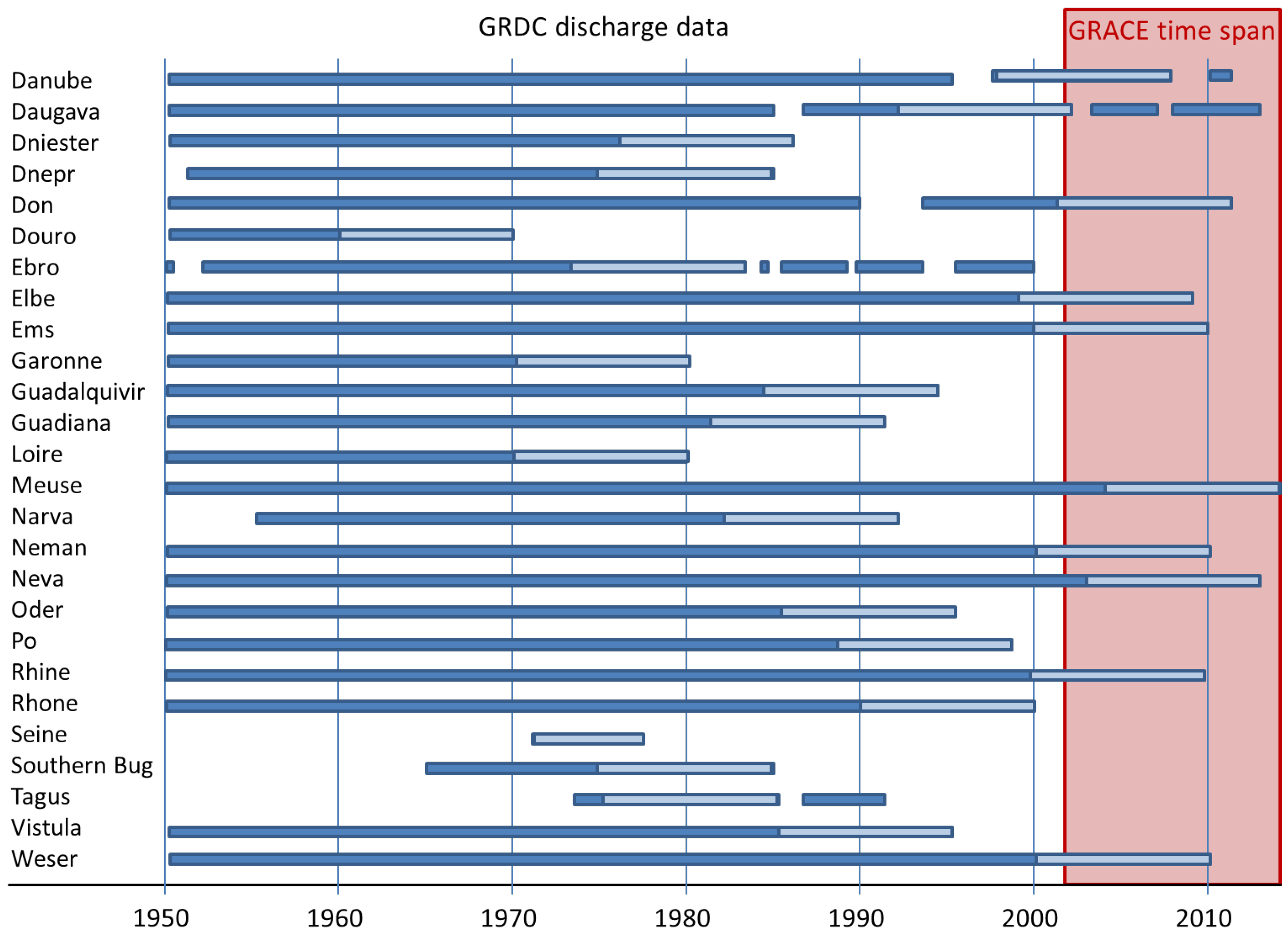
Figure 3.
Discharge R for the Rhine from Global Runoff Data Centre (GRDC) (blue) and simulated from Génie Rural rainfall-runoff model (GR2M)-snow (red) including the standard deviation (grey).
Figure 3.
Discharge R for the Rhine from Global Runoff Data Centre (GRDC) (blue) and simulated from Génie Rural rainfall-runoff model (GR2M)-snow (red) including the standard deviation (grey).
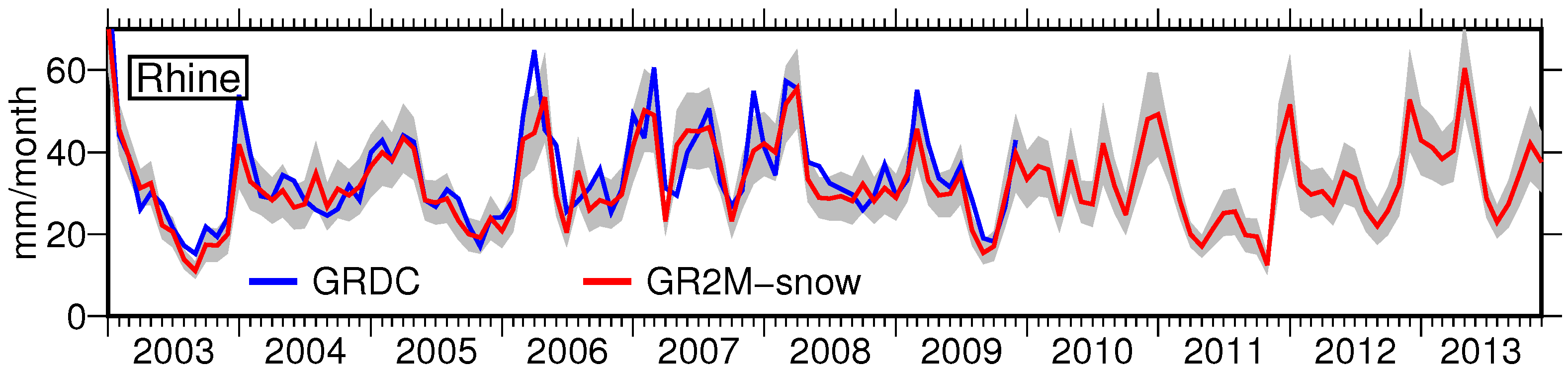
Figure 4.
Total water storage (TWS) change (red) and its standard deviation (grey) for two selected river basins.
Figure 4.
Total water storage (TWS) change (red) and its standard deviation (grey) for two selected river basins.
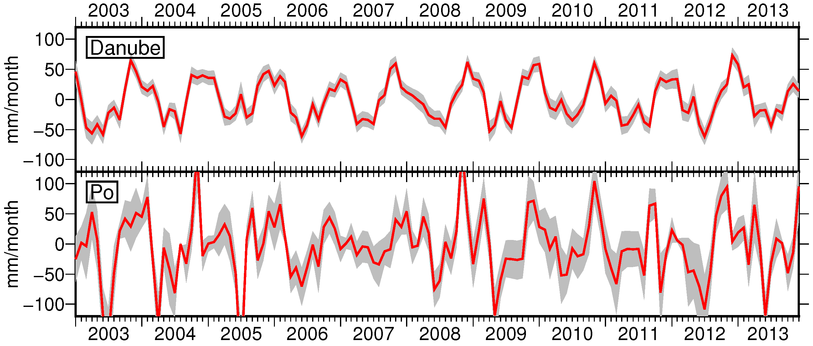
Figure 5.
Monthly total precipitation P from different models and simulated discharge R (black dashed) for selected catchments of the study area.
Figure 5.
Monthly total precipitation P from different models and simulated discharge R (black dashed) for selected catchments of the study area.
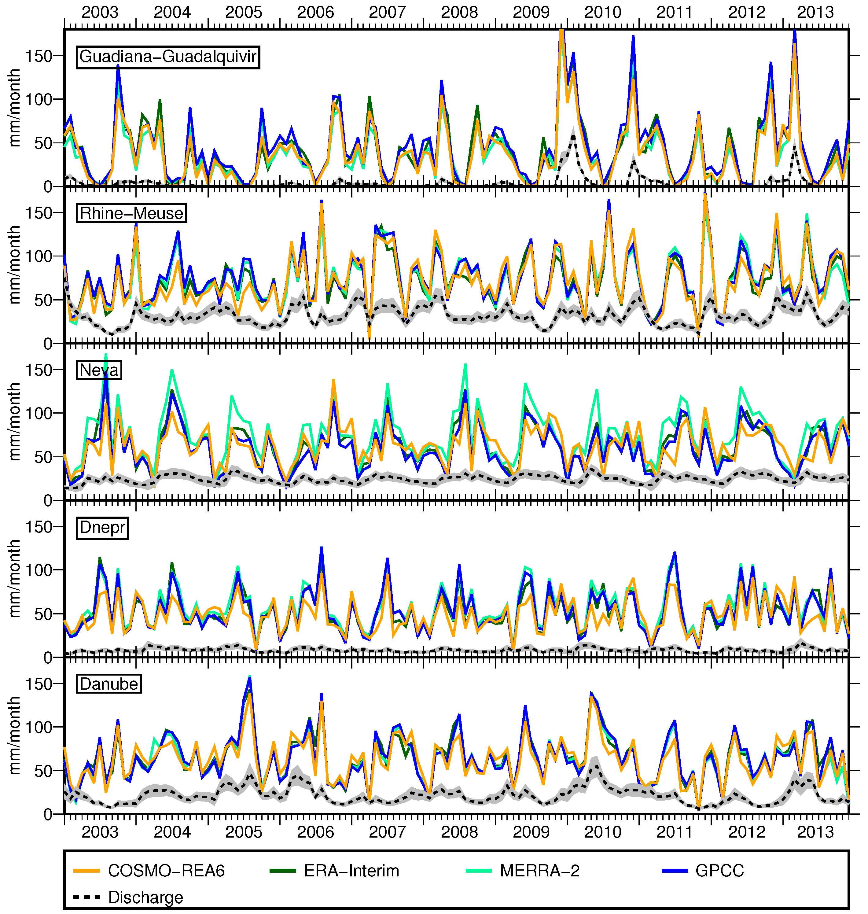
Figure 6.
Monthly total evapotranspiration E from different models for selected catchments of the study area.
Figure 6.
Monthly total evapotranspiration E from different models for selected catchments of the study area.

Figure 7.
The closure of the water budget equation is assessed for selected river basins. The left side of the equation is represented by the red line and includes propagated standard deviations (black). All time series are smoothed with a three-month moving average filter to facilitate interpretation.

Figure 8.
De-seasoned and de-trended time series of and (red) for selected river basins.

Figure 9.
Correlation of and from COSMO-REA6 Reanalysis for (a) the original time series, as shown in Figure 7, and (b) de-trended and de-seasoned time series, as shown in Figure 8.
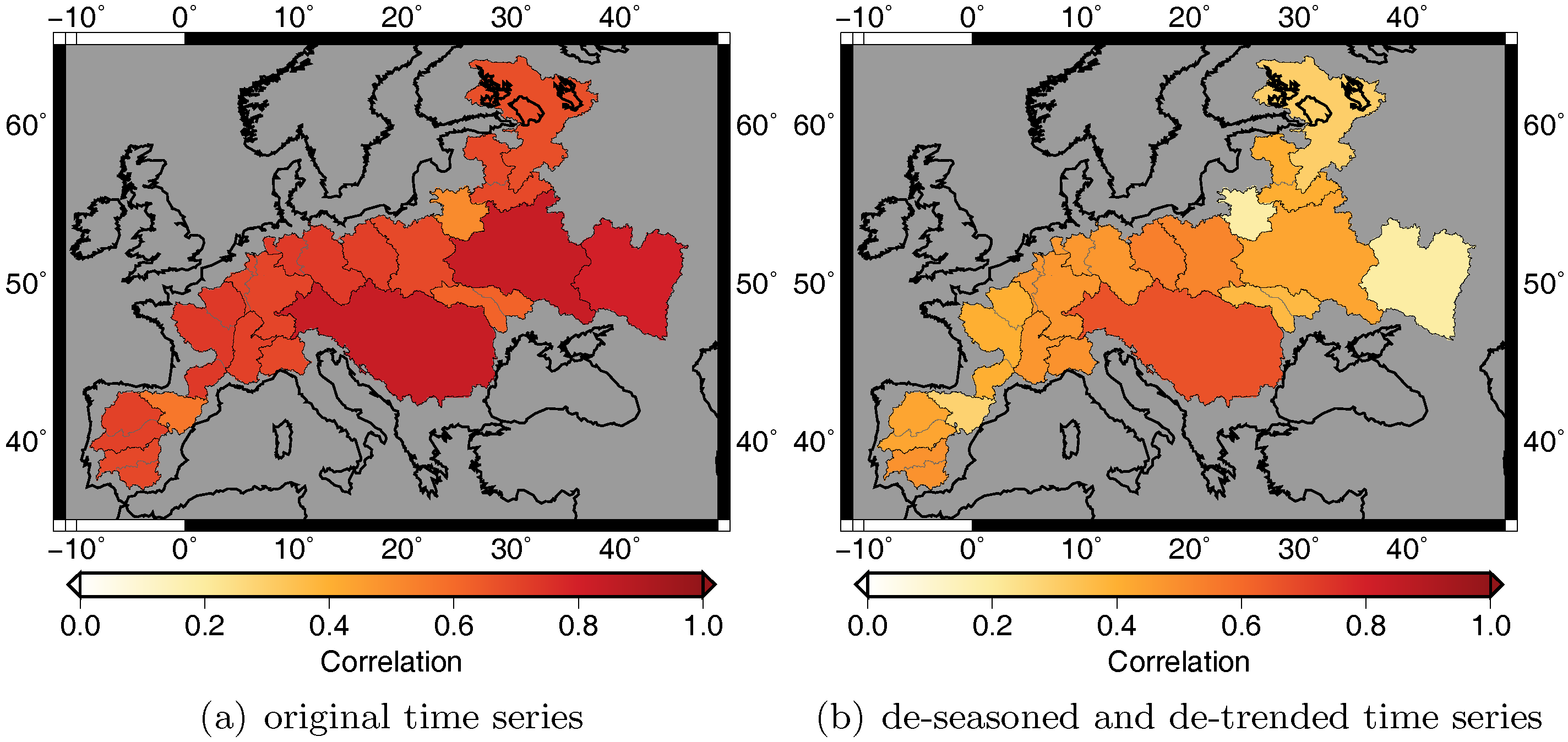
Figure 10.
(a–d) Bias of the water budget equation given in equivalent water height (EWH): red color means that is underestimated, and blue color means that is overestimated. (e) provides as a reference the propagated error of the left side of the water budget equation.
Figure 10.
(a–d) Bias of the water budget equation given in equivalent water height (EWH): red color means that is underestimated, and blue color means that is overestimated. (e) provides as a reference the propagated error of the left side of the water budget equation.

Figure 11.
Amplitudes of and given in equivalent water height (EWH).

Figure 12.
Trend of and given in equivalent water height (EWH).


Table 1.
The target catchments and their size.
| Catchment | Size (km) | Catchment | Size (km) |
|---|---|---|---|
| Danube | 807,000 | Meuse-Rhine | 180,601 |
| Daugava-Narva | 120,500 | Neman | 81,200 |
| Dnepr | 463,000 | Neva | 281,000 |
| Don | 378,000 | Oder | 109,729 |
| Douro-Tagus | 158,981 | Po | 70,091 |
| Ebro | 84,230 | Rhone | 95,590 |
| Elbe-Ems-Weser | 178,039 | Southern Bug-Dniester | 112,300 |
| Garonne-Loire-Seine | 227,000 | Vistula | 194,376 |
| Guadalquivir-Guadiana | 107,878 |
Table 2.
Evaluation of simulated discharge from GR2M-snow for the validation period of each river basin: mean values, mean standard deviation (Std.), root mean squared errors (RMSE), bias of the mean and Nash–Sutcliffe (NS) coefficients for time series with seasonal cycle and de-seasoned and de-trended (des., det.) time series are computed as defined in Section 3.2. Due to missing observations, no validation could be performed for Seine and Tagus (* Neman and Vistula are calibrated and validated using E-RUN (observational gridded runoff estimates for Europe) because of erroneous GRDC data).
| Catchment | Mean | Std. | RMSE | Bias | NS | NS |
|---|---|---|---|---|---|---|
| () | () | () | () | des., det. | ||
| Danube | 19.1 | 4.8 | 4.2 | 0.4 | 0.67 | −0.34 |
| Daugava | 18.0 | 7.9 | 9.1 | 0.9 | 0.60 | 0.28 |
| Dniester | 13.8 | 4.0 | 5.9 | −0.9 | 0.65 | 0.38 |
| Dnepr | 8.2 | 2.6 | 4.1 | −0.5 | 0.42 | 0.22 |
| Don | 4.8 | 1.7 | 2.1 | 0.2 | −0.12 | −0.22 |
| Douro | 11.0 | 2.9 | 6.2 | −1.0 | 0.61 | 0.45 |
| Ebro | 14.9 | 3.6 | 6.2 | 0.23 | 0.73 | 0.25 |
| Elbe | 11.9 | 3.1 | 4.2 | −0.1 | 0.69 | 0.17 |
| Ems | 28.3 | 5.6 | 9.8 | 1.6 | 0.84 | 0.49 |
| Garonne | 33.7 | 6.7 | 11.2 | 2.5 | 0.81 | 0.38 |
| Narva | 16.2 | 4.1 | 4.0 | 1.2 | 0.62 | 0.42 |
| Guadalquivir | 3.4 | 1.2 | 4.6 | −1.2 | 0.63 | 0.53 |
| Guadiana | 4.0 | 1.4 | 6.1 | −1.8 | 0.66 | 0.65 |
| Loire | 23.8 | 5.2 | 7.4 | 1.8 | 0.84 | 0.35 |
| Meuse | 35.2 | 7.4 | 11.0 | 1.7 | 0.84 | 0.50 |
| Neman * | 14.6 | 4.7 | 5.8 | −3.2 | 0.69 | 0.58 |
| Neva | 22.3 | 4.5 | 3.5 | −0.5 | 0.66 | −0.73 |
| Oder | 15.3 | 3.7 | 4.4 | 0.5 | 0.59 | 0.27 |
| Po | 61.4 | 16.4 | 20.4 | 4.0 | 0.51 | −0.11 |
| Rhine | 38.2 | 7.3 | 7.6 | 1.1 | 0.77 | 0.36 |
| Rhone | 51.1 | 11.8 | 10.6 | 1.7 | 0.76 | 0.45 |
| Southern Bug | 5.7 | 2.1 | 4.5 | −0.3 | 0.21 | 0.07 |
| Vistula * | 15.3 | 4.3 | 4.8 | −1.0 | 0.54 | 0.29 |
| Weser | 22.5 | 5.1 | 7.3 | 0.1 | 0.83 | 0.51 |
© 2017 by the authors. Licensee MDPI, Basel, Switzerland. This article is an open access article distributed under the terms and conditions of the Creative Commons Attribution (CC BY) license (http://creativecommons.org/licenses/by/4.0/).
Share and Cite
MDPI and ACS Style
Springer, A.; Eicker, A.; Bettge, A.; Kusche, J.; Hense, A. Evaluation of the Water Cycle in the European COSMO-REA6 Reanalysis Using GRACE. Water 2017, 9, 289. https://doi.org/10.3390/w9040289
AMA Style
Springer A, Eicker A, Bettge A, Kusche J, Hense A. Evaluation of the Water Cycle in the European COSMO-REA6 Reanalysis Using GRACE. Water. 2017; 9(4):289. https://doi.org/10.3390/w9040289
Chicago/Turabian StyleSpringer, Anne, Annette Eicker, Anika Bettge, Jürgen Kusche, and Andreas Hense. 2017. "Evaluation of the Water Cycle in the European COSMO-REA6 Reanalysis Using GRACE" Water 9, no. 4: 289. https://doi.org/10.3390/w9040289
Note that from the first issue of 2016, this journal uses article numbers instead of page numbers. See further details here.