
Pluvial Flooding in European Cities—A Continental Approach to Urban Flood Modelling


1
Newcastle University School of Civil Engineering and Geosciences, NE1 7RU Newcastle upon Tyne, UK
2
Willis Research Network, 51 Lime St., EC3M 7DQ London, UK
*
Author to whom correspondence should be addressed.
Water 2017, 9(4), 296; https://doi.org/10.3390/w9040296
Submission received: 8 February 2017
/
Revised: 6 April 2017
/
Accepted: 18 April 2017
/
Published: 22 April 2017
Abstract
:Pluvial flooding is caused by localized intense rainfall and the flood models used to assess it are normally applied on a city (or part of a city) scale using local rainfall records and a high resolution digital elevation model (DEM). Here, we attempt to model pluvial flooding on a continental scale and calculate the percentage of area flooded for all European cities for a 10-year return period for hourly rainfall (RP10). Difficulties in obtaining hourly rainfall records compromise the estimation of each city RP10 and the Europe-wide DEM spatial resolution is low relative to those typically used for individual case-studies. Nevertheless, the modelling capabilities and necessary computing power make this type of continental study now possible. This is a first attempt at continental city flooding modelling and our methodology was designed so that our results can easily be updated as better/more data becomes available. The results for each city depend on the interplay of rainfall intensity, the elevation map of the city and the flow paths that are created. In general, cities with lower percentage of city flooded are in the north and west coastal areas of Europe, while the higher percentages are seen in continental and Mediterranean areas.
1. Introduction
Pluvial flooding is caused by intense rainfall that exceeds the capacity of the urban drainage system and is normally studied using flood models that can provide depth and velocity of surface water associated with rainfall events of specified intensity [1]. These models are typically applied on a small area (a city, or often just a part of a city), using local rainfall records and a high resolution digital elevation model (DEM). Here we take advantage of emerging global datasets and cloud computing to provide a preliminary assessment of pluvial flood impacts for 571 cities across the continent of Europe.
Global or continental scale flood impact studies have previously been restricted to river or coastal flooding. To place this work in context it is relevant to assess the latest developments on large scale fluvial modelling.
Smith et al. [2] performed a regional flood frequency analysis (RFFA) at global scale using 703 discharge gauges from the Global Runoff Data Centre (GRDC) and a global annual average rainfall dataset from World-Clim [3]. Regressions were used to calculate the mean annual flood and they concluded that the best regressions used just catchment area and annual average rainfall as estimators. Different exponents for the two estimators were calculated for different climatic areas based on the Koppen–Geiger classification, where Europe is mainly constituted by temperate and continental classes. The regressions performed better for temperate, tropical and polar regions than the drier continental and arid regions. Also, means and medians of the relative mean square errors were substantially different, demonstrating the strong effect of a small number of poorly performing gauges. The authors hypothesise that this might be due to basins with extensive water abstraction. The mean error for the mean annual flood regression applied to temperate climate was 77% (median of 37%), and for continental climate this was 151% (44% median). The authors conclude that there is “some predictive skill” for the majority of the stations whilst pointing out that this methodology is not appropriate to provide estimates of detailed localized discharge.
Using the above RFFA, Sampson et al. [4] added information about the terrain and assumptions about the river channels in order to produce global flood hazard maps. However, this is not valid for channels in catchments with an area below 50 km2. Therefore, the authors estimated intensity–duration–frequency (IDF) curves based on approximately 200 gauges around the world (pooled together and then partitioned by the different climatic areas based on the Köppen–Geiger classification). Subsequently, the IDF curves for each climatic region were regressed using annual average rainfall in order to estimate extreme rainfall worldwide. Nevertheless, the authors consider this method fit-for-purpose, since despite the fact that local features will undeniably result in very significant errors on a local scale, the errors of the DEM used (Shuttle Radar Topography Mission, SRTM, DEM with a 3 arc second resolution ~90 m) are expected to be the dominant source of uncertainty of the hydrological model.
An alternative methodology is to model the whole of Europe with a hydrological model, but this requires vast amounts of data, much of which is not readily available at a European scale (e.g., aquifer characteristics). Despite the challenges of running and calibrating such a model, several studies of flooding in Europe have tried to use simple hydrological or hydraulic models. For example, Lisflood [5] requires inputs representing precipitation, air temperature, potential evapotranspiration, and evaporation from open water bodies and bare soil surfaces and has been run for the whole of Europe at 5-km resolution [6]. The model has been calibrated with data from 258 European catchments for at least four years of observed discharge with a focus on the timing and magnitude of flood events. However, results for daily discharge were far from ideal, with 70% of values at ±25%, 23% of the values below that interval (underestimation of discharges) and 7% above (overestimation of discharges).
Roudier et al. [7] also used pan-European hydrological models for flooding assessment, in this case Lisflood, E-Hype and VIC (Variable Infiltration Capacity). The models were run with bias corrected climate model simulations. The median of the 100-year discharge level (Q100) modelled was assessed against the Q100 calculated from 428 gauges (from several sources). Root-mean-square errors were lower for Lisflood (961 m3/s) than E-Hype (1124 m3/s) or VIC (1279 m3/s) but these differences in performance might be partly explained by different calibration methodologies and datasets.
Errors in simulation of pan-European historical discharges are substantial whether regression methodologies or hydrological models are used. Smith, Sampson and Bates [2] identified several problems with large scale river flood modelling, including:
- the quality of the available DEMs, especially in forested regions and urban areas where the satellite information might correspond to the top of the canopy/building instead of the elevation of the ground;
- the quality of the precipitation data, which is very variable in time and place, and the fact that different types of rainfall inputs (gauge, radar, satellite or reanalysis) results in different orders of magnitude in terms of monetary loss from flooding results;
- the lack of data to calibrate hydrological models, especially in ungauged catchments.
These challenges are also relevant in our assessment of urban flood impacts for 571 European cities. Furthermore, whereas for fluvial flooding daily observations are often sufficient for continental scale analysis, pluvial flooding required hourly observations. The restricted availability of observed hourly rainfall records which, coupled with the spatial variability of intense rainfall regimes, hinders the definition of historical intense rainfall return periods for each city. Projects like INTENSE (https://research.ncl.ac.uk/intense/aboutintense/) where worldwide hourly rainfall gauge data is being collated or frameworks like OPERA (http://eumetnet.eu/activities/observations-programme/current-activities/opera/) where pan-European weather radar composites are being produced will hopefully help to solve this problem in the future. Moreover, whereas statistical analysis or reduced process complexity flood model algorithms are useful for fluvial analysis, pluvial flood modelling requires a 2D physically-based model at high resolution in order to minimize statistical generalization and capture key flow paths and accumulation points. However, this requires a significant increase in computational effort particularly as each urban area is subject to different climatology, and a comprehensive analysis requires consideration of a range of rainfall intensities.
In this paper we present the first pan-European analysis of urban flooding. In Section 2 the data used for this study is introduced, followed by the methodology in Section 3. This includes both the methodology to estimate rainfall levels for each city for a 10-year return period (Section 3.1) and the methodology associated with the use of the urban hydrodynamic model (Section 3.2). Results and discussion are presented in Section 4, followed by conclusions in Section 5.
2. Data
Crucial for any broad scale modelling is the availability of consistent, continental-wide, data. Although a number of cities or countries have bespoke, and often higher resolution, data services, this analysis used the following Europe-wide data:
- EU-DEM [8]—a Digital Elevation Model over Europe “produced using Copernicus data and information funded by the European Union”. The EU-DEM is a hybrid product based on SRTM and ASTER GDEM data with 25-m resolution (projection 3035: EU-DEM-3035).
- Urban Morphological zones 2000 [10] defined as “set of urban areas laying less than 200 m apart”. This European Environment Agency (EEA) dataset was built based on the urban land cover classes of the CORINE Land Cover dataset. This data was necessary to define the “urban area” inside each city since the definition of “city” in the urban audit dataset can include non-urban areas, and sometimes even estuaries (see Figure S2 in Supplementary Materials for some examples).
- E-obs [11], an European daily gridded data set for precipitation and maximum and mean surface temperature at a 0.25 degree resolution for the period 1950–2013. E-obs is based on observations from 2316 stations, although the number changes over time showing a sharp rise in the number of gauges from 1950 to 1960 and a dip in 1976 (for stations with less than 20% missing monthly data). However, the spatial coverage throughout Europe is every uneven, with the UK, Ireland, the Netherlands and Switzerland having a much higher gauge density.
- Several observed sub-daily rainfall datasets were combined:
- -
- A total of 38 European gauges with time-series of annual maximum hourly rainfall, provided by Dr Panos Panagos, from the Joint Research Centre, that were collected under the auspices of the REDES project [12].
- -
- Some 192 UK gauges with time-series of annual maximum hourly rainfall (provided by Dr. Stephen Blenkinsop from Newcastle University) that were collected under the auspices of the CONVEX project [13]. These data were collected from three sources: the UK Met Office Integrated Data Archive System (MIDAS), the Scottish Environmental Protection Agency (SEPA) and the UK Environment Agency (EA). Not all these gauges were used, since that would mean the density of gauges used in the UK would be well above the density of gauges in the rest of Europe, therefore affecting the results of the analyses.
- -
- One gauge (Catraia) with hourly time-series for the South of Portugal downloaded from the Portuguese National Water Resources Information System (http://snirh.pt/).
- -
- IDF curves were collated for:
3. Methods
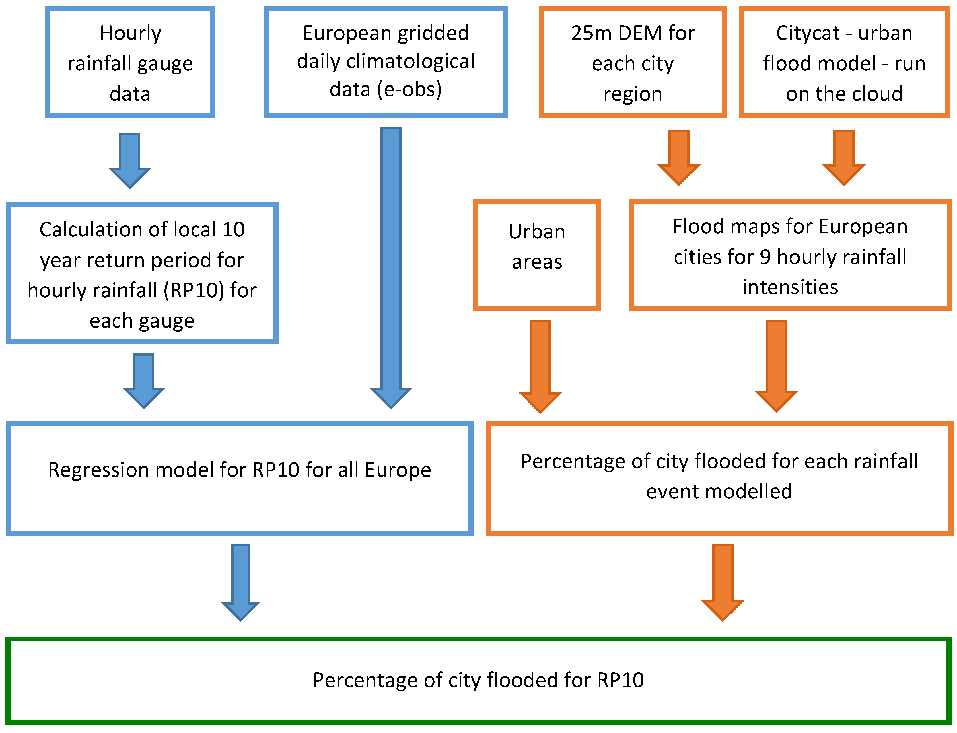
The methodology adopted is summarized in Figure 2 and comprises two parallel workflows. Hourly rainfall levels for a 10-year return period (RP10) were calculated for the whole of Europe (workflow in blue in Figure 2). For this, sub-daily rainfall datasets or IDF curves were compiled for as many European gauges as possible, and RP10 for each gauge were calculated. The 10-year return period was chosen, despite not being a very extreme rainfall event, due to the short rainfall records for some of the gauges and the consequent uncertainties associated with the calculation of longer return periods.
In parallel a physically-based flood model (CityCat) was run on the Microsoft Azure Cloud (Microsoft, Redmond, WA, USA) for all 571 European cities for nine different rainfall events (20 mm/h, 30 mm/h, 40 mm/h, 50 mm/h, 60 mm/h, 70 mm/h, 80 mm/h, 100 mm/h and 125 mm/h) using a DEM of 25 m (the highest-resolution DEM found for Europe). Using these maps, and a threshold of 5 cm of water depth to define an area as flooded, the percentage of city flooded was calculated. This percentage was based only on the urban area (Urban Morphological Zones, see Section 2).
A linear interpolation was applied between each of the modelled rainfall events to determine the proportion of city flooded for the historical hourly rainfall for a 10-year return period. The two workflows are now described in the subsequent sections.
3.1. Historical Intense Hourly Rainfall
The first step was to compile sub-daily rainfall datasets or IDF curves for as many sites in Europe as possible (see Section 2). Unfortunately, these data are not readily available and we were only able to collate data for 46 gauges, many of them with short records, which limits the reliability of our methods.
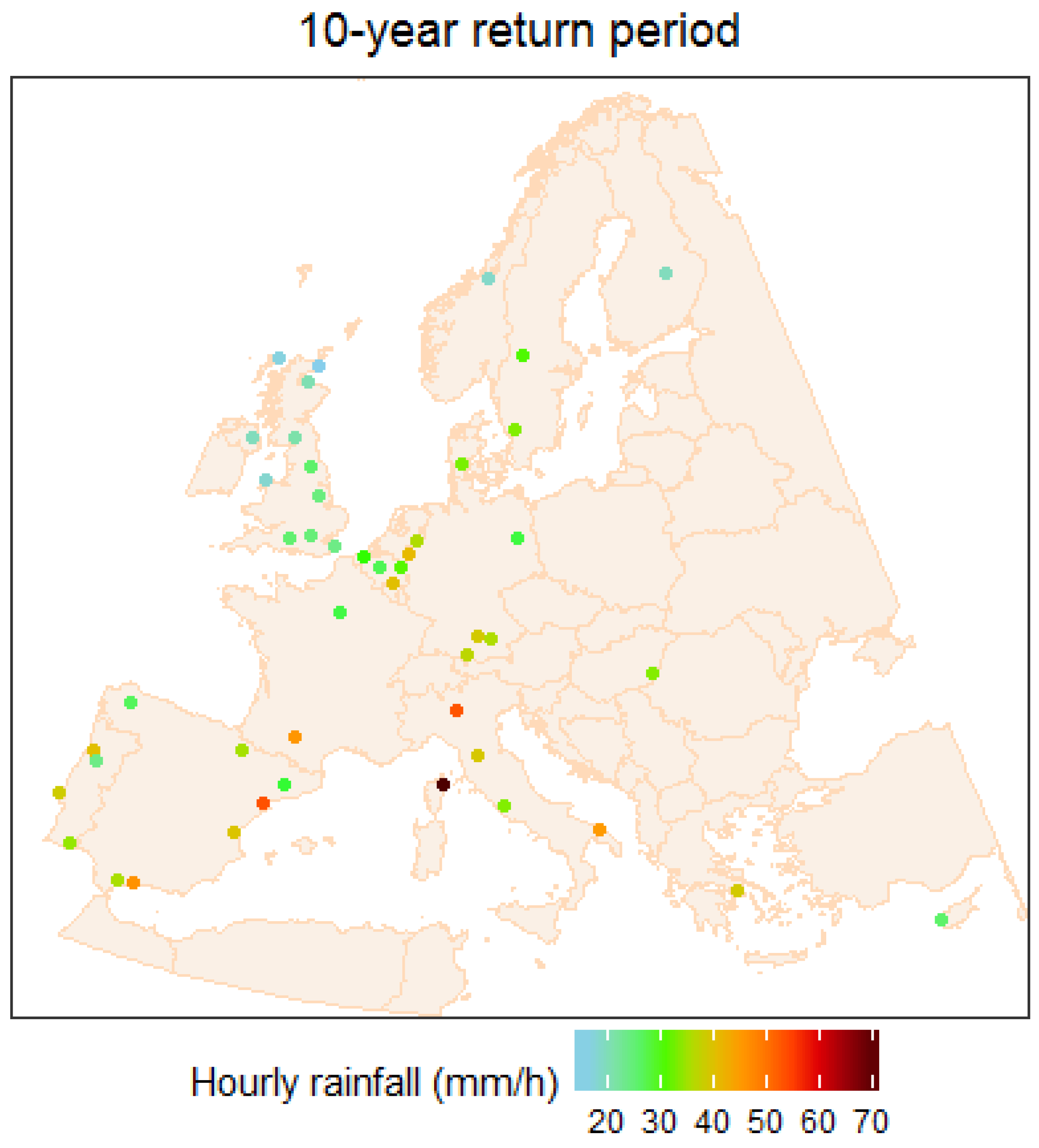
After the compilation, hourly levels of rainfall for a 10-year return period were calculated for all available time-series. This (not so extreme) return level was chosen in order to minimize the impact of the short length of some of the time-series used. Nonetheless, errors are still expected since the short time-series do not allow a proper characterization of the local climatology and the possible clustering of intense rainfall events shown by Willems [18]. Considering the data available, hourly annual maxima had to be used instead of peaks-over-threshold. Following normal practice, a GEV (Generalized Extreme Value) distribution was fitted to all gauges (using maximum likelihood estimation) and confidence intervals (95%) were calculated. A discretization correction factor (1.16) was applied to those data calculated from fixed window hourly time-series [19]. The resulting hourly rainfall levels for a RP10, as well as the number of years available per gauge for this calculation are shown in supplementary information (Figure S1). Figure 3 shows the spatial distribution of the calculated RP10. It is clear that the gauge in Corsica (Bastia) has a rainfall level for a 10-year return period (72 mm/h) well above all other gauges used in this study which vary between 14 mm/h and 54 mm/h. This is due to the unusual physiographic setting of the island which is well known for its frequent, very intense rainfall episodes [20].
Numerous regression models for estimating RP10 were tested using different climatological variables from E-obs (rainfall, maximum and minimum temperatures as daily, monthly and annual values) as well as elevation and location as predictor variables. In order to choose which predictors to use, the usual statistical measures of goodness of fit (R2, correlation between variables, predictive power of the used variables, and statistics of the residuals) were used. However, the robustness of the regression across possible ranges of values of predictors had to be carefully considered, since the model must be applied to all Europe. Therefore, lower R2 values and higher errors at each gauge were preferred to overfitting the regression to the available gauge data, which could result in unrealistic RP10 when the regression is applied throughout Europe.
The following regression equation was calculated:
where RP10 is hourly rainfall for a 10-year return period, is the median of the annual maximum daily rainfall, is the maximum monthly mean rainfall, and is the minimum monthly maximum temperature.
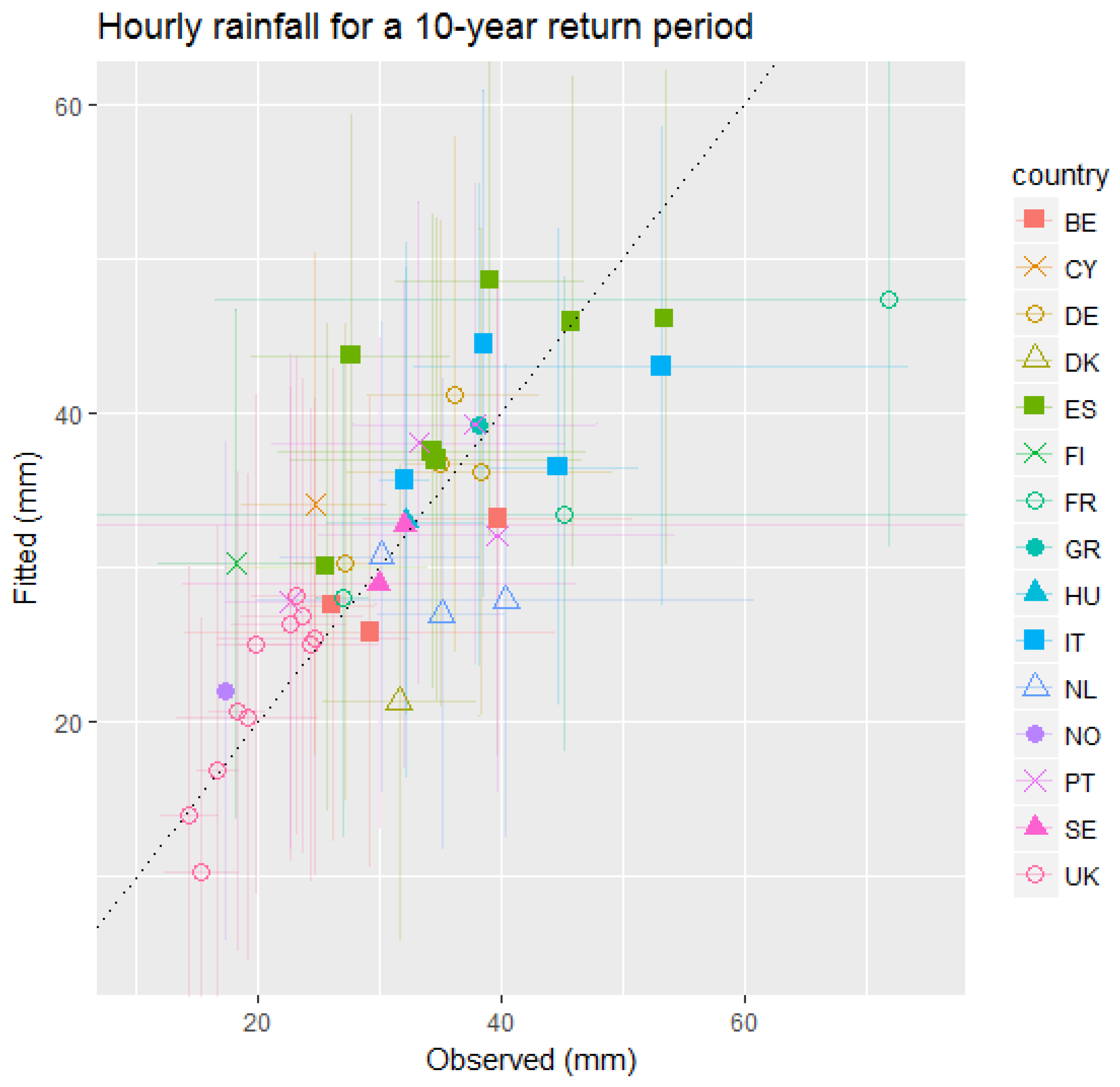
All the predictors are significant (all p-values below 0.006) and have low variance inflation factors (all below 4.4) meaning that the regression variables are not correlated; therefore, the model was considered robust. However, the R2 value is not very high (0.57) and the Bastia gauge has a large residual of 24.6 mm. Figure 4 shows maps of the residuals for all gauges. Figure 5 compares the observed and estimated RP10 for all gauges with the confidence intervals for the observed values. Here it can be seen that the confidence intervals for Bastia (green square on the top-right corner of the plot) are very large (the 10-year return period can be between 16 mm/h and 128 mm/h) which is due to the high interannual variability of the Mediterranean climate and the short record length (10 years of data). Removal of the Bastia record was considered due to the large confidence interval and residual but it was decided to be preferable to retain the data in this analysis as an example of the unusually intense rainfall regimes to be expected in some parts of Europe, and the inadequacy of this, and future, observing networks in characterizing them.
3.2. Urban Hydrodynamic Model
In parallel to the estimation of intense hourly rainfall, flood modelling was performed for all 571 cities using the urban flood model CityCat (City Catchment Analysis Tool) based on the 25-m resolution DEM. Newcastle University has developed the CityCat model which provides rapid simulation of urban hydrodynamics based on the solution of the shallow water equations using the method of finite volume with shock-capturing schemes [21,22,23]. The solution of the Riemann problem was obtained using the Osher–Solomon Riemann solver [24].
Usually the model represents flow over a surface comprising the ground surface as well as buildings. The buildings can play an important role when high-resolution grids are used to capture complex flow paths in urban areas. In CityCat the buildings are treated explicitly by using the “building hole approach” [25]. However, when the gaps between the buildings are smaller than the size of the numerical cells then blockages will be created in the domain. As a result, the buildings were not treated explicitly in the model because the resolution of the DEM is 25 m. Therefore, the flow fields will only be approximations of the true situation and the dynamics will be dominated by the overall topography rather than local effects of buildings. If more detailed data was available, such as a 2-m DEM and building outline shapefiles, then more realistic simulations would be achievable.
CityCat has an infiltration component based on the Green-Ampt method [26] where the soil hydraulic conductivity, suction head and porosity are used to estimate the infiltration rate in the permeable areas. However, in this work the infiltration was not taken into account due to the coarseness of the numerical. This is equivalent to the widely adopted (worst-case) assumption of saturated initial conditions.
While a complete urban flood assessment should include the sub-surface drainage network it is not feasible here for two reasons: (a) it is impossible to obtain detailed data for the drainage network for more than a handful of individual cities; and (b) fully coupled models for surface-subsurface drainage networks which can handle accurately free surface, mixed and pressurized flows are not currently available. Other approximate approaches to account for the impact of the networks are sometimes used. The simplest is to apply uniform losses, e.g., 12 mm/h allowance [27], but this takes no account of the efficiency or spatial variability of networks. A more detailed approach generates synthetic networks based on topography and building density information [28], but again requires a large effort in development, data and computation. For these reasons the drainage networks were not taken into account in this work, and it should be recognized that the flood extents are therefore over-estimates, more so for the smaller rainfall depths than for the largest, where the sub-surface networks will be overwhelmed.
The rainfall events used to run CityCat were generated following the Flood Estimation Handbook procedure [29] where an intense “summer profile” was used with duration of one hour. The need for spatially variable rainfall inputs instead of uniform “blanket” rainfall is an active research topic [30,31]. There is an open question on the relative importance of the geometry of the topographic and drainage network against the spatial pattern of rainfall. However, the use of spatial rainfall is severely restricted by the absence of suitable high-resolution rainfall data [32] and so in this study we have used uniform rainfall. Spatial rainfall effects could be assessed by running simulations for each city driven by an ensemble of stochastic rainfall model scenarios [33,34] but with major implications for computational cost.
For this study, the CityCat model was deployed on the Microsoft Azure Cloud and a parameter sweep platform was used to simultaneously carry out simulations for 571 cities, each for a range of 9 hourly rain storms of different magnitudes. Currently the standard platform for parameter sweeps jobs in the Microsoft Azure Cloud is the Azure Batch which is available as a service. This service provides jobs scheduling so there is no need to specially develop schedulers, job queues and scaling of the virtual machines (VMs) which Azure comprises. The steps we used for the setup of the parameter sweep jobs were: (a) uploading the data and the application to a storage server; (b) creating a pool of VMs; (c) creating jobs and tasks for the pool of VMs; and (d) calling a script for each task, with a set of parameters to configure and run the application. Once a task is completed the results are uploaded to a storage server and the VMs terminated after the completion of the jobs.
To perform the simulations for the 571 cities, a pool of 40 VMs was created, each with 112 GB of RAM and 16 cores. By running the tasks in parallel on each virtual machine the total simulation run-time reduced to approximately 2 days; by contrast, this would have taken approximately 80 days to perform these simulations on a single server.
As an example, the simulation result for Vienna for a 70 mm/h event is shown in Figure 6. The simulation results for every European city are available at http://ceg-research.ncl.ac.uk/ramses/.
The use of a coarse DEM, albeit with the highest resolution currently available for all of Europe, and the lack of a European building and sewer database increases the uncertainty in the flooded area estimates. Nevertheless, the model captures the movement of the water that results from the geography of the urban terrain.
The maximum water depth values for each rainfall event were calculated for all the grid cells in order to have a map of maximum flood depths for each city and each rainfall event. Subsequently, the percentage of city flooded for each event was calculated in order to construct event curves (percentage of area flooded for each rainfall intensity). For this, a threshold of 5 cm of flood depth was considered as defining the flooded area. Different thresholds could have been defined, since the threshold is dependent on what effects of flooding are of interest and the specificities of local construction. However, VanKirk [35] concluded that vehicles travelling in a depth of 5 cm or more of water are at risk of losing control and this was the threshold chosen for this study. Despite the whole city region being modelled with CityCat, the percentage of city flooded was calculated based only on the urban area (Urban Morphological Zones calculated based on CORINE—see Section 2) inside the “city region” defined in the Urban Audit dataset. This was a necessary step since some “city regions” are not appropriate for this type of analysis, with some even including estuary areas (examples are shown in supplementary information—Figure S2).
Linear interpolation was used to calculate flood impact between each of the simulated rainfall events, and to establish the percentage of city flooded by the historical hourly rainfall for the 10-year return period. Hypsometric curves—cumulative distribution functions of elevations—were calculated for each city using the 25-m DEM and possible relations with flooded areas investigated.
4. Results and Discussion
The hourly rainfall for the RP10, calculated using the regression model in Equation (1), for all of Europe is shown in Figure 7. RP10 could not be calculated for Malta because as a small island it is incompatible with the coarser resolution of the e-obs dataset. Northern Europe, especially the Atlantic coast, has the lowest rainfall intensities (with the exception of Norway). The Mediterranean area, especially the Pyrenees and Alps regions, shows the highest rainfall intensities for the 10-year return period. This map should be seen as a rough guide to RP10 in Europe due to the small number of gauges available for its calculation and the short records of some of those gauges.
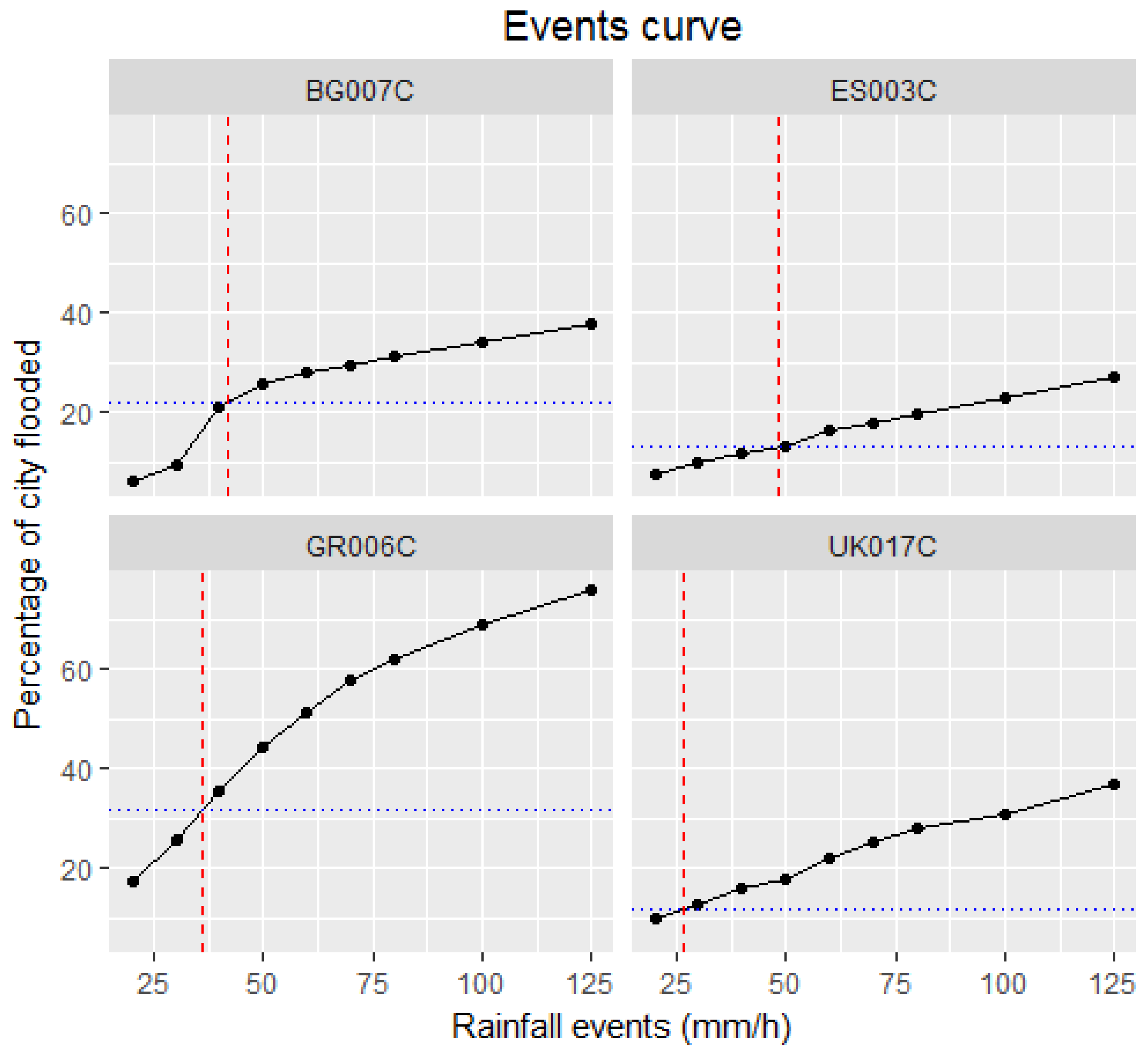
Figure 8 shows four example of pluvial flood impact functions for four cities (proportion of urban area flooded as a function of rainfall magnitude) calculated from the CityCat modelling. The RP10 for each city is also shown. Curves for all European cities are shown in the supplementary information (in Figure S3 the flooded area is defined as the area having at least 5 cm of flood depth, whereas Figure S4 has an alternative threshold of 50 cm of flood depth), and these four have been chosen as indicative of different types of impact function and different RP10 values.
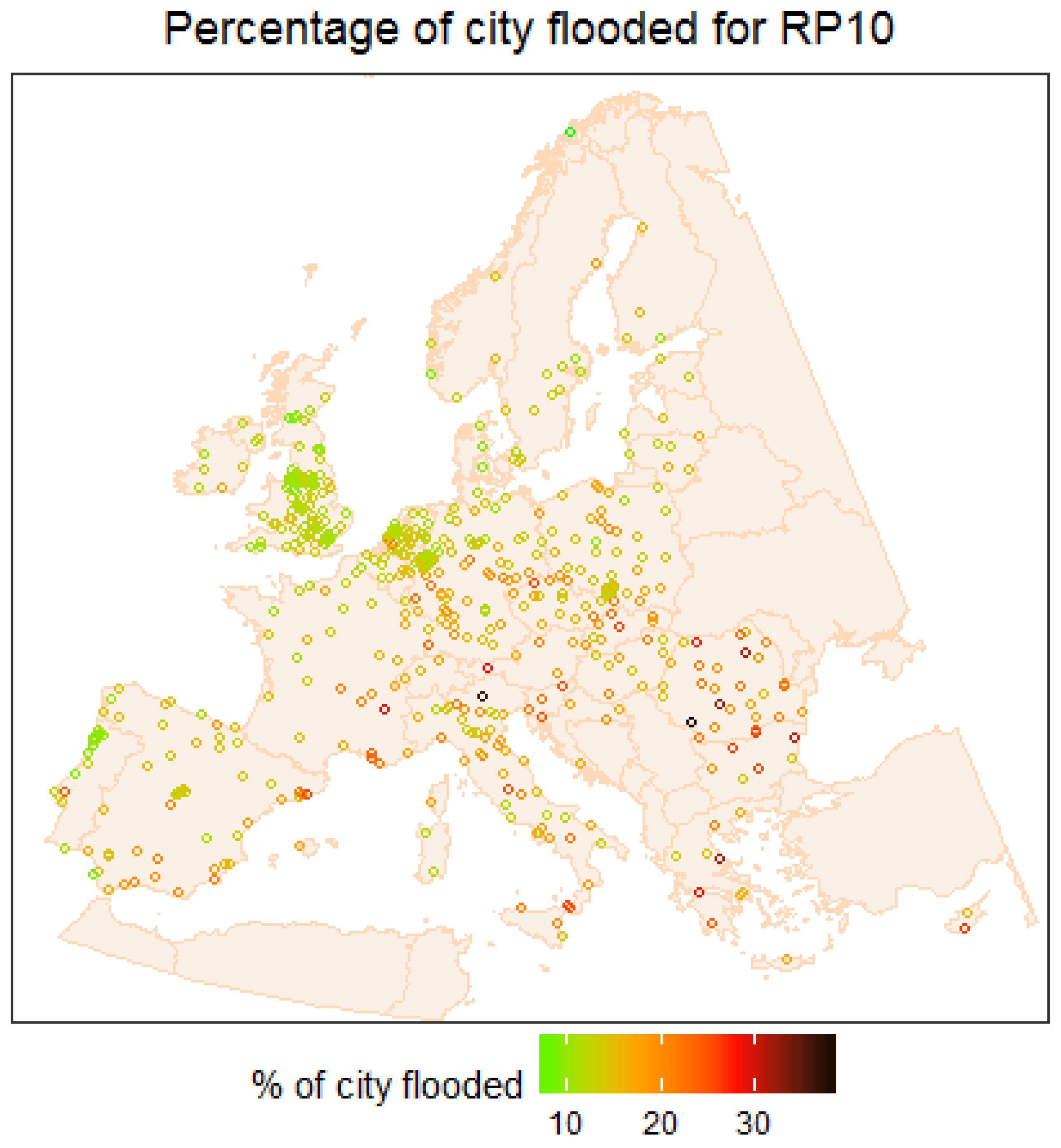
Figure 9 shows the percentage of city flooded associated with their hourly rainfall for the 10-year return period, which was calculated using each pluvial flood impact function.
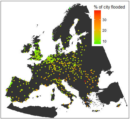
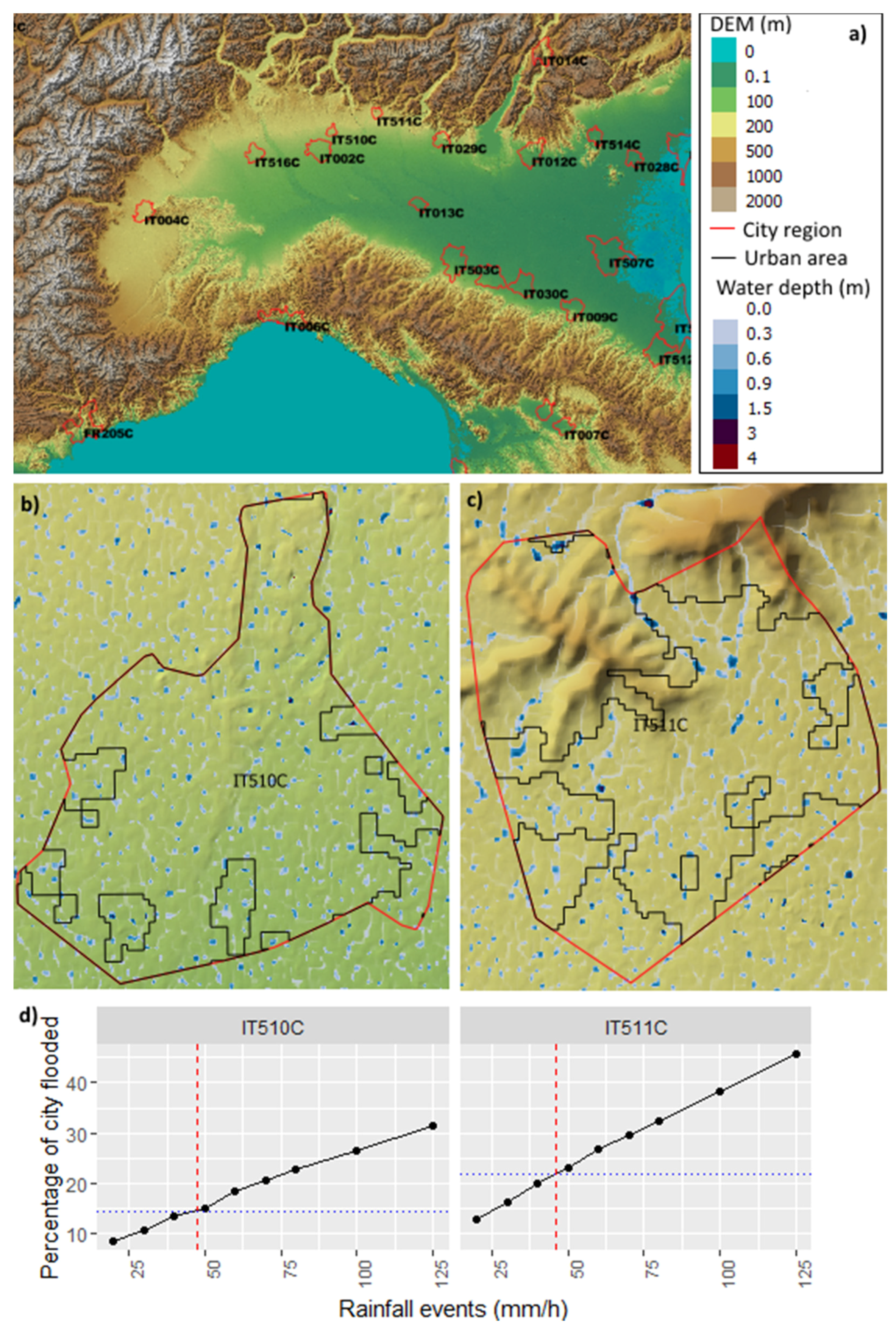
Most of the cities showing a high percentage of city flooded are in areas of high rainfall intensity and most of the cities showing low percentage of area flooded are in areas of low rainfall intensity. However, that is not always the case, since the flooded area is the result of the interplay of the rainfall intensity, urban elevation and topography, flow paths (which are a result of the former variables) and the area being analysed (the “urban area” inside the “city region”). Figure 10 exemplifies this, where two cities (IT510C—Monza and IT511C—Bergamo) with almost the same RP10 (47 mm/h and 46 mm/h respectively) have considerably different percentages of city flooded (14% and 22%) due to differences in the elevations and flow paths.
In order to see if these results could be reproduced (or at least approximated) using just a DEM, without recurring to a flood model, a comparison between hypsometric curves and the pluvial flood impact functions (for the same elevation range) was investigated.
Correlation between the slopes of the hypsometric curves and the slopes of the pluvial flood impact functions were weak and negative (−0.52 using Spearman’s rank correlation coefficient, see Figure S5). As the hypsometric curves and the events curves are not correlated, we concluded that elevation is a poor proxy for estimating the area of a city that will get flooded by a rainfall event. Therefore, a process-based flood model, like the CityCat model used here, is essential to assess pluvial flood impacts, even for the broad-scale analysis implemented here.
5. Conclusions
Here we have presented a first continental scale analysis of pluvial flood impacts in urban areas. We calculated the percentage of city flooded for 571 European cities, based on their RP10 calculated using a Europe-wide regression model of a composite of best available data.
Difficulties were encountered in terms of data availability, mainly for hourly rainfall records which compromises the estimation of each city RP10. Data availability also means that a simplified flood modelling approach has to be used, which does not account for local sewer systems, building shapes or infiltration occurring in local green spaces. Also, the best available DEM with European coverage has a relatively coarse spatial resolution (25 m) which is far below ideal for this type of study—although it improves upon the 90-m resolution used in many large scale fluvial and coastal assessments. Nevertheless, via use of a workflow that harnesses cloud computing we have shown that the modelling and analytical capabilities required for broad scale pluvial impacts modelling are now feasible.
Because our methodology consisted of two paralleled workflows (RP10 estimation for the whole Europe and physically-based flood modelling of all 571 European cities for nine different rainfall events using CityCat) each of these workflows can be improved separately. For example, if hourly rainfall records improve across Europe the estimation of RP10 could be improved, and the results could be updates without the need to run CityCat again. Similarly, if a higher-resolution DEM and building data became available for all 571 cities, the flood impact function could be efficiently recalculated by scaling the number of processors requested from the cloud resource.
Analysis of our results showed that urban flooding is the result of the interplay of rainfall intensity, the elevation map of the city and the flow paths that are created and could not be replicated using a simple elevation or gradient relationship. Therefore, a process-based flood model is required even for the broad-scale pluvial flood impacts analysis undertaken here.
Although local factors prohibit an absolute generalization, most of the cities with lower percentage of city flooded are in the north and west coastal areas of Europe, while the higher percentages are predominately in continental and Mediterranean areas.
Supplementary Materials
The following are available online at www.mdpi.com/2073-4441/9/4/296/s1, Figure S1: Number of years available for each gauge (left) and distribution of 10-year return period hourly rainfall (right). Figure S2: Examples of different definitions of “city”. In black is the “city region” as defined in the Urban Audit dataset, in red the Urban Morphological zones calculated based on CORINE. On the left several cities in the Amsterdam (NL002C) area are shown, the top-right shows Cagliari (IT027C) and the bottom right map shows Aveiro (PT008C). Figure S3. Cities’ pluvial flood impact functions—percentage of city flooded (meaning a height of water above 5 cm) per rainfall event. Figure S4: Cities pluvial flood impact functions—percentage of city flooded (meaning a height of water above 50 cm) per rainfall event. Figure S5: Relationship between the gradients of the clipped hypsometric curves and the gradient of the pluvial flood impact functions for each city. Contour lines are added (in blue) to help the perception of point density which was not clear with the 571 points.
Acknowledgments
This research has received funding from the European Union’s Seventh Programme for Research, Technological Development and Demonstration under Grant Agreement No. 308497 (Project RAMSES). The CityCAT model development was partly carried out under the Engineering and Physical Sciences Research Council grant EP/K013661/1 "Delivering and evaluating multiple flood risk benefits". We would like to thank Kenji Takeda and Microsoft for providing us support and access to the Microsoft Azure cloud platform under the Azure for Research Award program. We would also like to thank Panos Panagos, from the Joint Research Centre for providing annual maximum hourly rainfall series for 38 European gauges collected under the auspices of the REDES project.
Author Contributions
Selma Guerreiro processed all the data, calculated the RP10s, analysed the results and wrote most of the paper; Vassilis Glenis ran all the CityCat modelling on the cloud and wrote part of the methodology, Richard Dawson and Chris Kilsby supervised the research, and all authors revised the paper.
Conflicts of Interest
The authors declare no conflict of interest.
References
- Glenis, V.; McGough, A.S.; Kutija, V.; Kilsby, C.; Woodman, S. Flood modelling for cities using cloud computing. J. Cloud Comput. 2013, 2, 7. [Google Scholar] [CrossRef]
- Smith, A.; Sampson, C.; Bates, P. Regional flood frequency analysis at the global scale. Water Resour. Res. 2015, 51, 539–553. [Google Scholar] [CrossRef]
- Hijmans, R.J.; Cameron, S.E.; Parra, J.L.; Jones, P.G.; Jarvis, A. Very high resolution interpolated climate surfaces for global land areas. Int. J. Climatol. 2005, 25, 1965–1978. [Google Scholar] [CrossRef]
- Sampson, C.C.; Smith, A.M.; Bates, P.D.; Neal, J.C.; Alfieri, L.; Freer, J.E. A high-resolution global flood hazard model. Water Resour. Res. 2015, 51, 7358–7381. [Google Scholar] [CrossRef] [PubMed]
- Van der Knijff, J.M.; Younis, J.; de Roo, A.P.J. Lisflood: A gis-based distributed model for river basin scale water balance and flood simulation. Int. J. Geogr. Inf. Sci. 2010, 24, 189–212. [Google Scholar] [CrossRef]
- Rojas, R.; Feyen, L.; Bianchi, A.; Dosio, A. Assessment of future flood hazard in Europe using a large ensemble of bias-corrected regional climate simulations. J. Geophys. Res. Atmos. 2012, 117. [Google Scholar] [CrossRef]
- Roudier, P.; Andersson, J.C.M.; Donnelly, C.; Feyen, L.; Greuell, W.; Ludwig, F. Projections of future floods and hydrological droughts in europe under a +2 °C global warming. Clim. Chang. 2016, 135, 341–355. [Google Scholar] [CrossRef]
- European Environment Agency (EEA). Digital Elevation Model over Europe (EU-DEM). Available online: http://www.eea.europa.eu/data-and-maps/data/eu-dem (accessed on 12 December 2014).
- Geodatabase URAU_2004; GISCO Urban Audit, European Commission, Eurostat: Luxembourg, 2004.
- European Environment Agency (EEA). Urban Morphological Zones 2000. Available online: http://www.eea.europa.eu/data-and-maps/data/urban-morphological-zones-2000-2 (accessed on 18 June 2014).
- European Climate Assessment & Dataset (ECAD). E-Obs Data Portal. Available online: http://www.ecad.eu/download/ensembles/download.php (accessed on 25 November 2013).
- Panagos, P.; Ballabio, C.; Borrelli, P.; Meusburger, K.; Klik, A.; Rousseva, S.; Tadić, M.P.; Michaelides, S.; Hrabalíková, M.; Olsen, P.; et al. Rainfall erosivity in Europe. Sci. Total Environ. 2015, 511, 801–814. [Google Scholar] [CrossRef] [PubMed]
- Blenkinsop, S.; Lewis, E.; Chan, S.C.; Fowler, H.J. Quality control of an hourly precipitation dataset and climatology of extremes for the UK. Clim. Chang. 2017, 37, 722–740. [Google Scholar]
- Koutsoyiannis, D.; Baloutsos, G. Analysis of a long record of annual maximum rainfall in athens, greece, and design rainfall inferences. Nat. Hazards 2000, 22, 29–48. [Google Scholar] [CrossRef]
- Ayuso-Muñoz, J.L.; García-Marín, A.P.; Ayuso-Ruiz, P.; Estévez, J.; Pizarro-Tapia, R.; Taguas, E.V. A more efficient rainfall intensity-duration-frequency relationship by using an “at-site” regional frequency analysis: Application at Mediterranean climate locations. Water Resour. Manag. 2015, 29, 3243–3263. [Google Scholar] [CrossRef]
- Pérez-Zanón, N.; Casas-Castillo, M.C.; Rodríguez-Solà, R.; Peña, J.; Rius, A.; Solé, J.G.; Redaño, Á. Analysis of extreme rainfall in the Ebre observatory (Spain). Theor. Appl. Climato. 2016, 124, 935–944. [Google Scholar] [CrossRef]
- Hailegeorgis, T.T.; Thorolfsson, S.T.; Alfredsen, K. Regional frequency analysis of extreme precipitation with consideration of uncertainties to update IDF curves for the city of Trondheim. J. Hydrol. 2013, 498, 305–318. [Google Scholar] [CrossRef]
- Willems, P. Multidecadal oscillatory behaviour of rainfall extremes in Europe. Clim. Chang. 2013, 120, 931–944. [Google Scholar] [CrossRef]
- Faulkner, D. Rainfall frequency estimation. In Flood Estimation Handbook; Institute of Hydrology: Lancaster, UK, 1999. [Google Scholar]
- Lambert, D.; Argence, S. Preliminary study of an intense rainfall episode in Corsica, 14 September 2006. Adv. Geosci. 2008, 16, 125–129. [Google Scholar] [CrossRef]
- Harten, A.; Lax, P.D.; van Leer, B. On upstream differencing and godunov-type schemes for hyperbolic conservation laws. SIAM Rev. 1983, 25, 35–61. [Google Scholar] [CrossRef]
- Godunov, S.K. Finite difference method for numerical computation of discontinuous solutions of the equations of fluid dynamics. Mat. Sb. 1959, 47, 271–306. [Google Scholar]
- Toro, E.F. Riemann Solvers and Numerical Methods for Fluid Dynamics: A Practical Introduction; Springer: Berlin, Germany, 2013. [Google Scholar]
- Osher, S.; Solomon, F. Upwind difference schemes for hyperbolic conservation laws. Math. Comput. 1982, 38, 339–374. [Google Scholar] [CrossRef]
- Schubert, J.E.; Sanders, B.F.; Smith, M.J.; Wright, N.G. Unstructured mesh generation and landcover-based resistance for hydrodynamic modeling of urban flooding. Adv. Water Resour. 2008, 31, 1603–1621. [Google Scholar] [CrossRef]
- Kutílek, M.; Nielsen, D.R. Soil Hydrology; Catena Verlag: Cremlingen, Germany, 1994. [Google Scholar]
- Environment Agency (UK). What Is the Updated Flood Map for Surface Water? Environment Agency: Bristol, UK, 2013; Available online: https://www.gov.uk/government/uploads/system/uploads/attachment_data/file/297432/LIT_8988_0bf634.pdf (accessed on 5 April 2017).
- Sitzenfrei, R.; Möderl, M.; Rauch, W. Assessing the impact of transitions from centralised to decentralised water solutions on existing infrastructures—Integrated city-scale analysis with vibe. Water Res. 2013, 47, 7251–7263. [Google Scholar] [CrossRef] [PubMed]
- Institute of Hydrology. Flood Estimation Handbook, Volume 3: Statistical Procedures for Flood Frequency Estimation; Institute of Hydrology: Wallingford, UK, 1999. [Google Scholar]
- Ochoa-Rodriguez, S.; Wang, L.-P.; Gires, A.; Pina, R.D.; Reinoso-Rondinel, R.; Bruni, G.; Ichiba, A.; Gaitan, S.; Cristiano, E.; van Assel, J.; et al. Impact of spatial and temporal resolution of rainfall inputs on urban hydrodynamic modelling outputs: A multi-catchment investigation. J. Hydrol. 2015, 531, 389–407. [Google Scholar] [CrossRef]
- Gires, A.; Giangola-Murzyn, A.; Abbes, J.-B.; Tchiguirinskaia, I.; Schertzer, D.; Lovejoy, S. Impacts of small scale rainfall variability in urban areas: A case study with 1D and 1D/2D hydrological models in a multifractal framework. Urban Water J. 2015, 12, 607–617. [Google Scholar] [CrossRef]
- Berne, A.; Delrieu, G.; Creutin, J.-D.; Obled, C. Temporal and spatial resolution of rainfall measurements required for urban hydrology. J.Hydrol. 2004, 299, 166–179. [Google Scholar] [CrossRef]
- Blanc, J.; Hall, J.W.; Roche, N.; Dawson, R.J.; Cesses, Y.; Burton, A.; Kilsby, C.G. Enhanced efficiency of pluvial flood risk estimation in urban areas using spatial—Temporal rainfall simulations. J. Flood Risk Manag. 2012, 5, 143–152. [Google Scholar] [CrossRef]
- Burton, A.; Glenis, V.; Bovolo, C.I.; Blenkinsop, S.; Fowler, H.J.; Chen, A.S.; Djordjevic, S.; Kilsby, C.G. Stochastic rainfall modelling for the assessment of urban flood hazard in a changing climate. In Proceedings of the British Hydrological Society’s Third International Symposium, Newcastle, UK, 19–23 July 2010; pp. 39–45. [Google Scholar]
- VanKirk, D.J. Vehicular Accident Investigation and Reconstruction; CRC Press: Boca Raton, FL, USA, 2000. [Google Scholar]
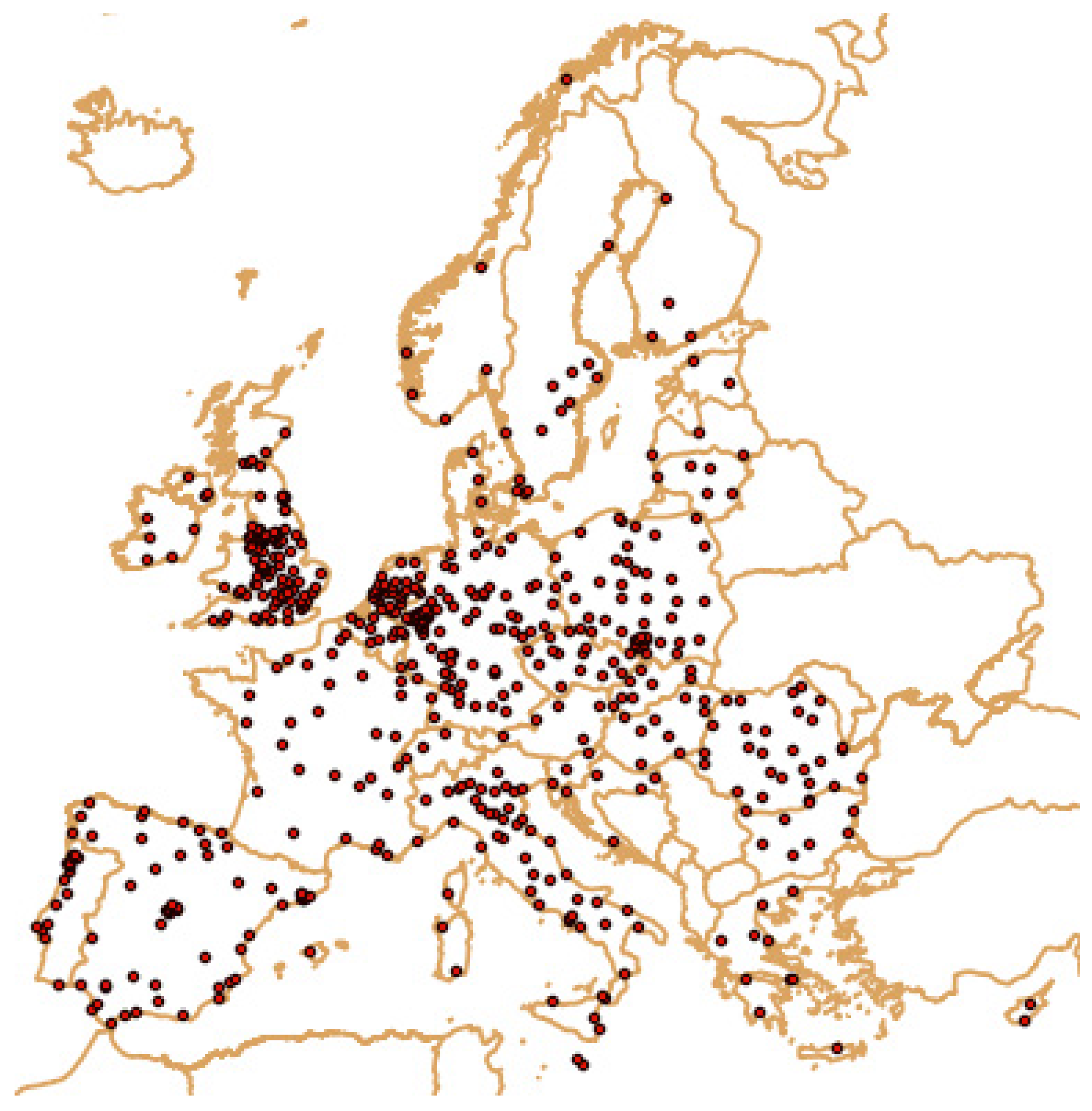
Figure 1.
Map of Europe with the cities from Urban Audit that were studied.

Figure 2.
Methodology flowchart.

Figure 3.
Map of Europe with the hourly rainfall for a 10-year return period for all available gauges. Return periods were calculated assuming a GEV (Generalized Extreme Value) distribution for all gauges. The number of years available for each gauge varied between 6 and 63 (median = 17 years).
Figure 3.
Map of Europe with the hourly rainfall for a 10-year return period for all available gauges. Return periods were calculated assuming a GEV (Generalized Extreme Value) distribution for all gauges. The number of years available for each gauge varied between 6 and 63 (median = 17 years).

Figure 4.
Maps of Europe showing the residuals of the linear regressions used to estimate the hourly rainfall for a 10-year return period. (a) Shows absolute residuals (in millimetres) while (b) shows relative residuals (calculated as a percentage of the observed rainfall level for a 10-year return period).
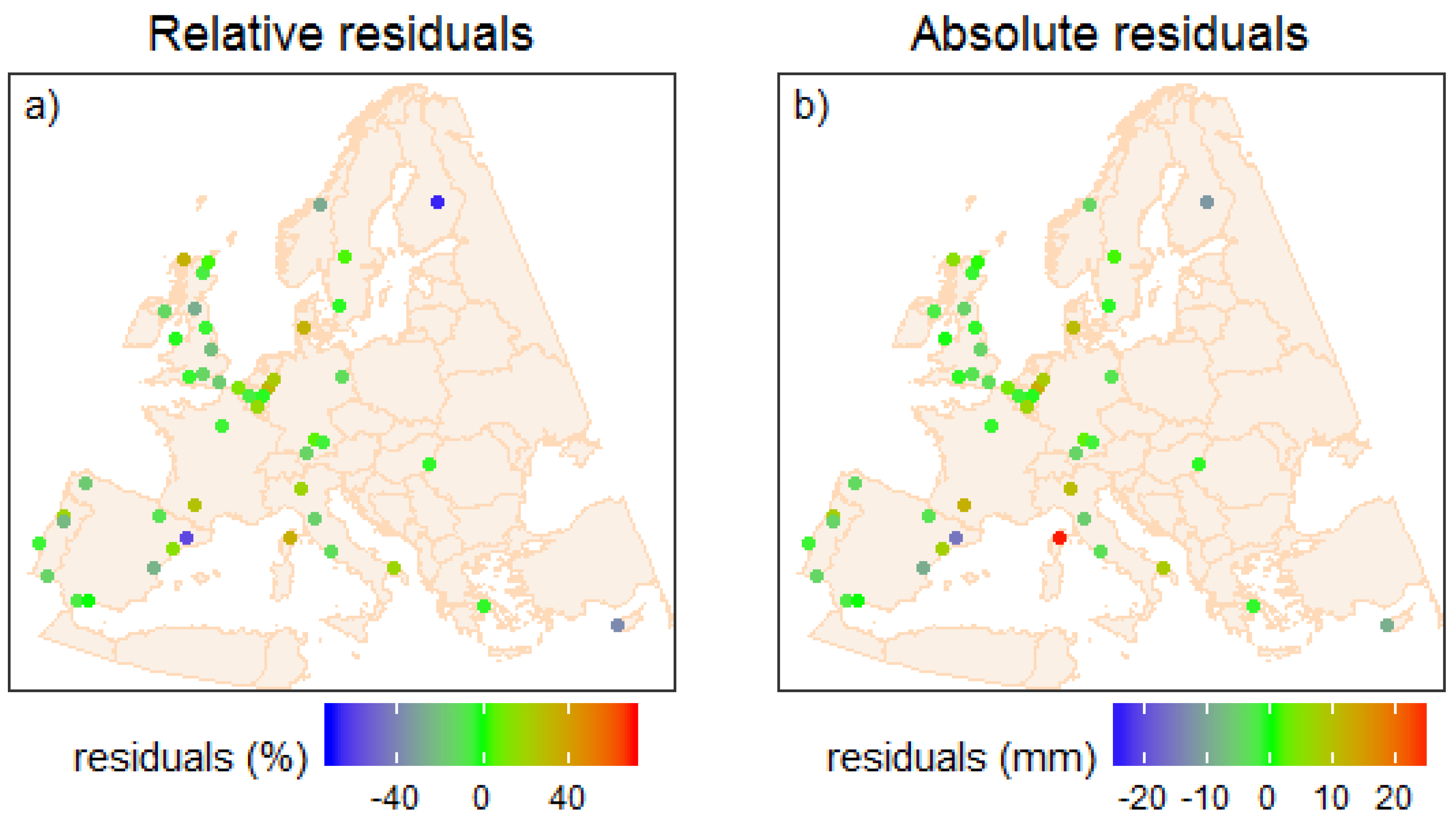
Figure 5.
Observed Vs estimated hourly rainfall for a 10-year return period for all gauges. When possible, the observed values are shown with their respective 0.05 confidence interval (horizontal lines). For four gauges (Athens, Barcelona, Firenze and Málaga) confidence intervals are not available because the time-series for these gauges were not available and their 10-year return period rainfall was retrieved from the literature (published intensity–duration–frequency (IDF) curves). Predictive intervals (0.95 level) are also shown (vertical lines). The diagonal dotted line shows the 1:1 line.

Figure 6.
CityCat (City Catchment Analysis Tool) flood maps for Vienna using a 70-mm/h storm (base map: Map data—Google, DigitalGlobe).
Figure 6.
CityCat (City Catchment Analysis Tool) flood maps for Vienna using a 70-mm/h storm (base map: Map data—Google, DigitalGlobe).
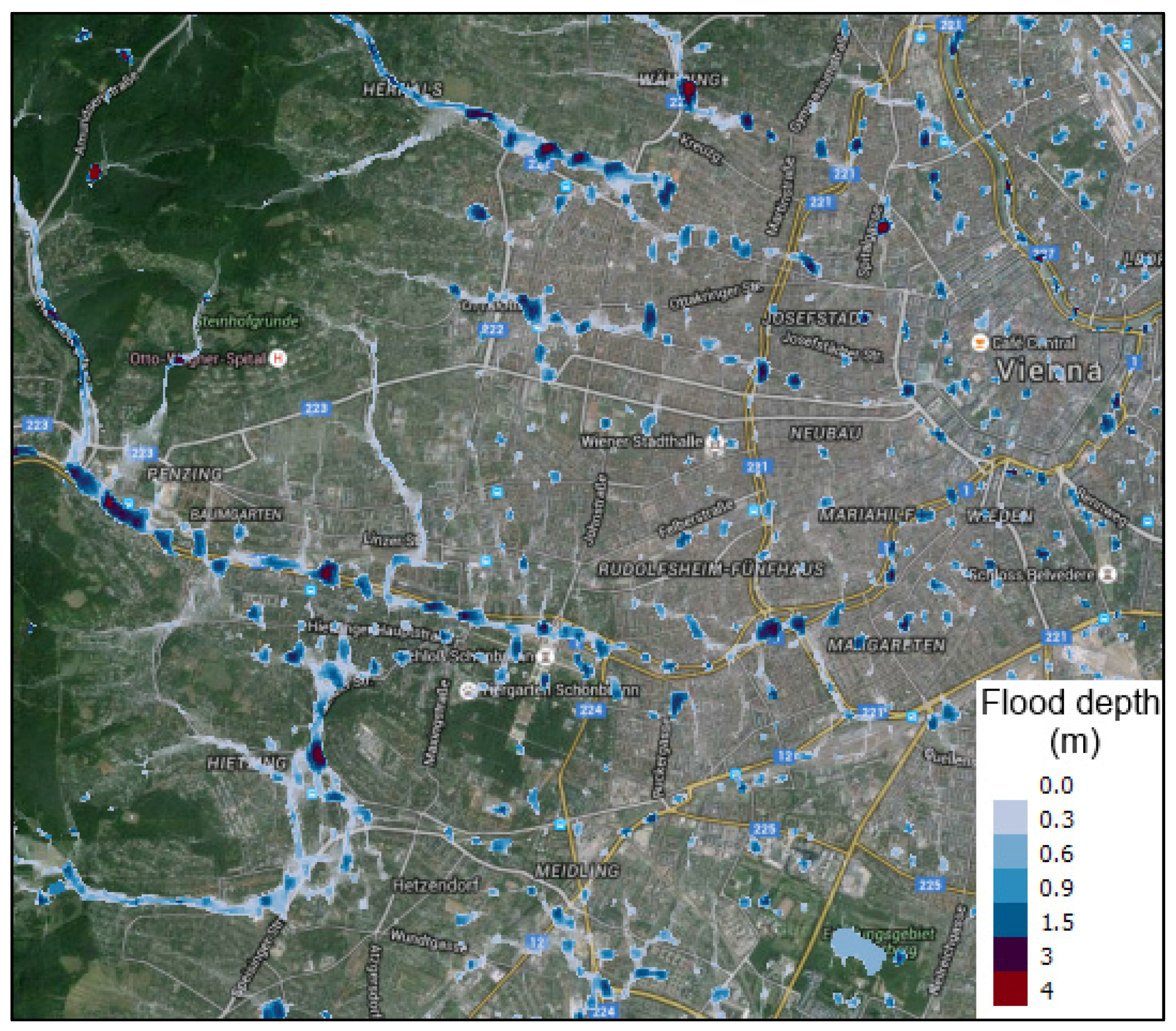
Figure 7.
Map of Europe showing the estimates from the regression model for hourly rainfall for a 10-year return period. The locations of the gauges used are shown as black dots.
Figure 7.
Map of Europe showing the estimates from the regression model for hourly rainfall for a 10-year return period. The locations of the gauges used are shown as black dots.
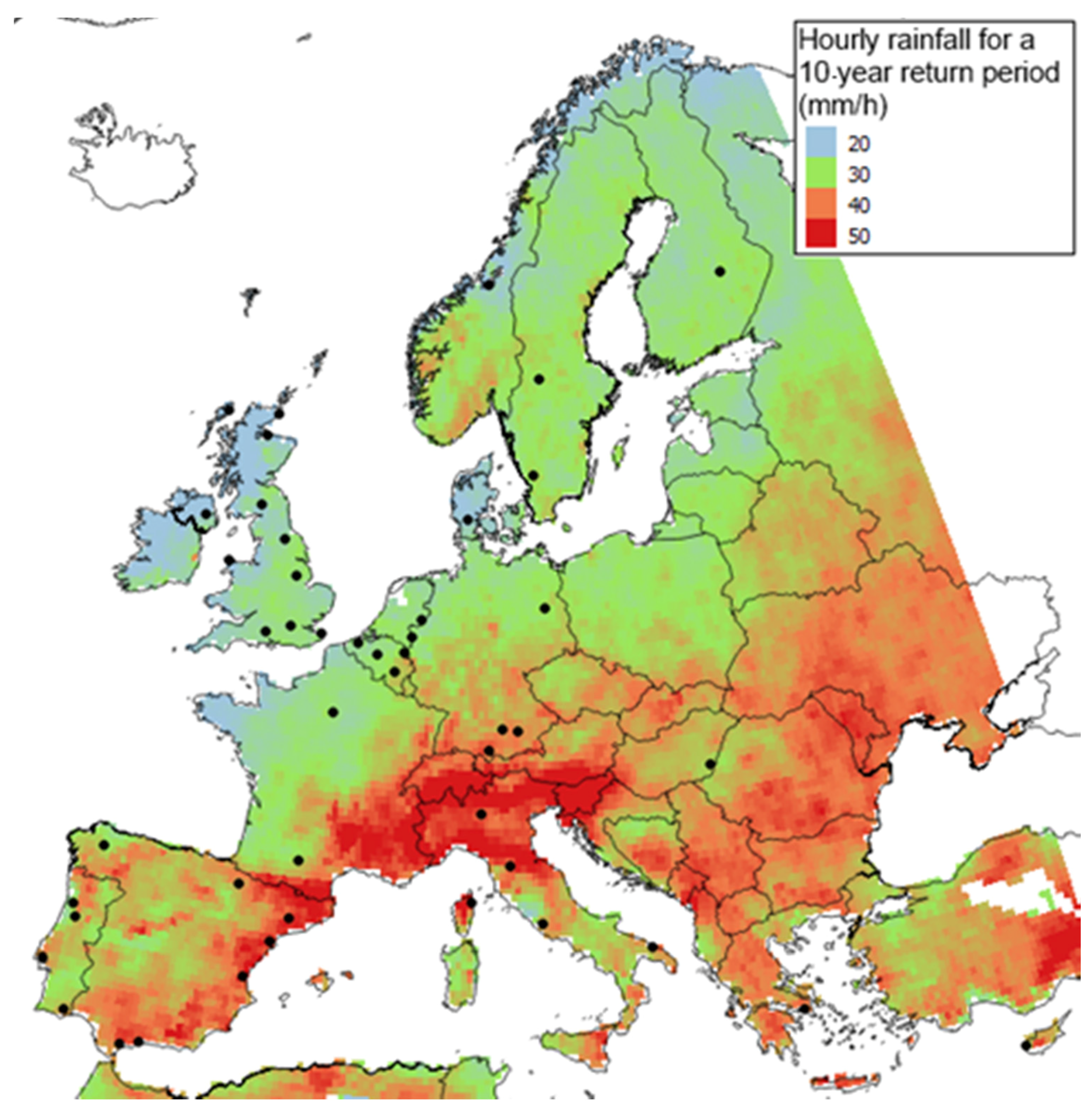
Figure 8.
Example of events curves for four cities: BG007C—Vidin (Bulgaria), ES003C—Valencia (Spain), GR006C—Volos (Greece), and UK017C—Cambridge (UK) calculated from the CityCat results. The red vertical dashed line shows the RP10 (hourly rainfall for a 10-year return period) and the dotted blue line shows the corresponding percentage of city flooded.

Figure 9.
Percentage of city flooded for historical hourly rainfall for a 10-year return period. These percentages are based on the rainfall event and the elevation map used for each city and do not have in consideration adaptation measures already implemented in these cities (like sewer systems) which will be different in different cities.

Figure 10.
Map of northern Italy with location of cities (a); flood maps of IT510C—Monza (b) and IT511C—Bergamo (c) and the cities’ pluvial flood impact functions—percentage of city flooded (meaning a height of water above 5 cm) per rainfall event (d). These two cities were chosen to exemplify how very similar RP10s can result in considerably different percentages of flooding.
© 2017 by the authors. Licensee MDPI, Basel, Switzerland. This article is an open access article distributed under the terms and conditions of the Creative Commons Attribution (CC BY) license (http://creativecommons.org/licenses/by/4.0/).
Share and Cite
MDPI and ACS Style
Guerreiro, S.B.; Glenis, V.; Dawson, R.J.; Kilsby, C. Pluvial Flooding in European Cities—A Continental Approach to Urban Flood Modelling. Water 2017, 9, 296. https://doi.org/10.3390/w9040296
AMA Style
Guerreiro SB, Glenis V, Dawson RJ, Kilsby C. Pluvial Flooding in European Cities—A Continental Approach to Urban Flood Modelling. Water. 2017; 9(4):296. https://doi.org/10.3390/w9040296
Chicago/Turabian StyleGuerreiro, Selma B., Vassilis Glenis, Richard J. Dawson, and Chris Kilsby. 2017. "Pluvial Flooding in European Cities—A Continental Approach to Urban Flood Modelling" Water 9, no. 4: 296. https://doi.org/10.3390/w9040296
Note that from the first issue of 2016, this journal uses article numbers instead of page numbers. See further details here.