
Flood Loss Models and Risk Analysis for Private Households in Can Tho City, Vietnam

1
GFZ German Research Centre for Geosciences, Section 5.4 Hydrology, 14473 Potsdam, Germany
2
Geography Department, Humboldt University, Berlin 12489, Germany
3
Southern Institute for Water Resources Research, Ho Chi Minh City 750062, Vietnam
*
Author to whom correspondence should be addressed.
Water 2017, 9(5), 313; https://doi.org/10.3390/w9050313
Submission received: 24 February 2017
/
Revised: 17 April 2017
/
Accepted: 24 April 2017
/
Published: 29 April 2017
(This article belongs to the Special Issue Innovative Aspects in Flood Risk Evaluation, Mapping and Communication)
Abstract
:Vietnam has a long history and experience with floods. Flood risk is expected to increase further due to climatic, land use and other global changes. Can Tho City, the cultural and economic center of the Mekong delta in Vietnam, is at high risk of flooding. To improve flood risk analyses for Vietnam, this study presents novel multi-variable flood loss models for residential buildings and contents and demonstrates their application in a flood risk assessment for the inner city of Can Tho. Cross-validation reveals that decision tree based loss models using the three input variables water depth, flood duration and floor space of building are more appropriate for estimating building and contents loss in comparison with depth–damage functions. The flood risk assessment reveals a median expected annual flood damage to private households of US$3340 thousand for the inner city of Can Tho. This is approximately 2.5% of the total annual income of households in the study area. For damage reduction improved flood risk management is required for the Mekong Delta, based on reliable damage and risk analyses.
1. Introduction
Due to global change, the frequency and intensity of flood hazards are expected to increase, particularly in coastal areas [1,2,3]. Additionally, population growth, rapid socio-economic development, and urbanization increase the exposure and susceptibility to floods in Vietnam [2]. Therefore, flood risk in Vietnam is high [3]. Can Tho City is situated beside the Hau river, a branch of the Mekong, which is only about 80 km from the sea. The city is the economic and cultural center of the Mekong delta and is influenced by tidal floods from the sea, by riverine floods from upstream, and by pluvial floods [4,5]. In addition, uncontrolled urbanization and a low capacity of the drainage infrastructure further increase the flood risk [6]. For instance, the flood in 2011 inundated about 27,800 houses and caused a loss of US$11.3 million in Can Tho City [7].
A reliable analysis of flood risk is essential for the development of an efficient and sustainable flood risk management, including investment decisions about flood control measures. One important part of flood risk analysis is flood loss modeling [8]. Many models are developed to estimate flood loss for different sectors of the economy, especially for residential buildings [9]. The available flood loss models are developed following an empirical and/or synthetic approach. The empirical approach uses loss data collected after flood events, while the synthetic approach uses what-if questions to collect data [10]. Both approaches have advantages and disadvantages. A combination of both approaches is useful, e.g., a synthetic model may be used to extend empirical data, or empirical data are used to evaluate synthetic models [10]. In addition, the loss models result either in an absolute monetary loss to assets or in a relative loss, i.e., the percentage of loss (loss/asset value) or an index value [11].
Traditionally, flood loss models are depth–damage functions, which describe the relationship between loss and inundation depth. Depth–damage functions are applied in many regions to estimate flood loss, for example depth–damage curve for urban areas in Australia [12]; frequency-damage estimation in USA [13]; depth–damage curve for residential built up area in Erasinos basin in Greece [14]; and depth–damage functions for private households and service sectors in Germany [15]. However, Merz et al. [15] and Thieken et al. [11] have shown that flood loss is influenced by many factors and hence, if assessment models consider only one parameter, the results are associated with large uncertainty, because inundation depth describes only a part of the variability of loss data.
Going beyond depth–damage functions, several models were developed considering some other flood characteristics such as duration, flow velocity or resistance characteristics such as building type, building quality or private precaution [11,16,17]. Multi-variable flood loss models using tree-based data mining approaches significantly improve loss modeling [18,19].
Some flood loss models have been developed for Vietnam. The Mekong River Commission [20], for example, developed a loss model for buildings in the Dong Thap and An Giang provinces based on water depth. Vo T.D. et al. [21] developed models to estimate both direct and indirect losses of households in Can Tho City considering flood-information exchange, level of flooding, gender, education, age, income, and migration. Vu T.T. [22] developed a flood loss model for buildings and contents in the Quang Ngai province based on building density, water depth, and average building value. The model of the Mekong River Commission [20] is appropriate for a quick and general assessment of flood losses. Although Vo T.D. et al. [21] provide a comprehensive loss assessment, they did not consider potentially important flood loss influencing parameters, which were found to be specifically important for the flood characteristic in the Mekong Delta, particularly, inundation duration [23,24]. The model by Vu T.T. [22] is particularly suitable for fast floods in large-scale areas but less suitable for slow and long-lasting floods in urban areas.
In order to address the above-mentioned shortcomings, this study aims to develop multivariable flood loss models for private households in urban areas, specifically for Can Tho City in the Mekong delta. To reach this objective, the paper describes and examines different methods in developing flood loss models for residential buildings and contents. Then, the paper presents model validation and how the developed models are used in a flood risk analysis. The core research questions addressed are the following:
- -
- Among the available methods, which one provides the best result for developing flood loss models for residential buildings and contents in Can Tho city?
- -
- How can flood risk in data scarce conditions such as in Can Tho City be analyzed?
This paper is organized as follows: Section 2 describes the case study and data used for developing flood loss models for residential buildings and contents in Can Tho City as well as for applying these models in a flood risk analysis. Section 3 describes the methodologies used to develop flood loss models and analyze flood risk, which is followed by a presentation of results and discussion in Section 4 and conclusion in Section 5.
2. Case Study
2.1. Case Study
Can Tho City is one of five cities in Vietnam that is controlled directly by the national government of Vietnam. The city is the economic, cultural and governmental center of the Vietnamese lower Mekong delta. Can Tho City is located on the western bank of the Hau river, a branch of the Mekong river. The city is located in the center of the Mekong delta, just 169 km away from Ho Chi Minh city, the biggest city in Vietnam. Can Tho has a convenient transportation system including harbor and airport, which makes it the national and international traffic hub of the Mekong delta. With an area of 1409 square kilometer, the city has about 1.2 million inhabitants, with 0.8 million inhabitants living in the urban and peri-urban area and 0.4 million inhabitants living in the rural area [25]. There are five urban districts consisting of Ninh Kieu, Binh Thuy, Cai Rang, O Mon and Thot Not and four rural districts namely Phong Dien, Thoi Lai, Vinh Thanh, Co Do (Figure 1). The city center is the Ninh Kieu district, which hosts governmental institutions, and commercial, financial, bank, educational and health services.
The topography of Can Tho City is flat with altitudes ranging from 0.6 to 1.2 m above sea level. There are two main rivers, namely Can Tho river and Hau River, and various smaller natural rivers and a dense system of channels [26]. The channel system is connected to the Hau River along the city and it provides fresh water for residential and manufacturing needs as well as waterway transportation through the city. The dike system is low, with the main purpose of protecting agriculture from flooding. The residential buildings are located mostly along the roads or right on the bank of rivers and channels.
Located in tropical and monsoonal climate, Can Tho City has hot and humid weather both in the rainy and dry season. The rainy season lasts from May to November, which provides 90% of the annual rainfall [27]. The dry season lasts from December to April with very low rainfall. Can Tho is about 80 km away from the sea. However, due to flat topography, the city is highly influenced by the tide. The high tide period in Can Tho City is from September to February [28]. Because of its location next to rivers that are influenced by the tide, Can Tho is affected by different types of flood, which often occur from September to November. Deep fluvial floods occur mainly in rural and peri-urban areas. Mixed floods resulting from fluvial, tidal and pluvial floods occur in urban areas, particularly in Ninh Kieu, Binh Thuy, and Cai Rang districts. In addition, floods in Can Tho City are also influenced by urbanization and infrastructure development. The largest recent flood in Can Tho City occurred in 2011, with two large fluvial events occurring between 26 September and 2 October, and between 24 and 31 October 2011.
This study performs a risk analysis for the most densely urbanized area in Can Tho city, which includes Ninh Kieu district and part of Binh Thuy district.
2.2. Data to Develop Loss Models
The development of flood loss models for residential buildings in Can Tho City is based on the empirical dataset that has been compiled from interview results [23,24] after the flood event of 2011. We use 858 damage cases (both houses with exclusive residential use and houses with small business) to develop flood loss models for residential buildings, and contents. The input data were collected via interviews, which covered the following topics: flood hazard characteristics of the 2011 flood event, flood preparedness, flood warning and emergency measures, flood loss to households and business contents, building structures and losses due to business interruption, risk perceptions, and the business and socio-economic characteristics of the respondents. The building damage was estimated from all damaged single construction parts of the building. Similarly, the contents damage refers to all items stored in the house, including furniture, home appliances, vehicles and electric items that were damaged by the flood. Detailed descriptions of the survey and the data processing were provided in Chinh et al. [23,24]. The important factors influencing residential flood loss in Can Tho have been analyzed and revealed to be: inundation duration, water depth, building value (or content value), floor space of the building, income and socio-economic status of the household. A detailed description of this multivariate analysis was given in Chinh et al. [24].
On basis of these results, we use the four most important loss determining parameters to develop flood loss models for residential buildings and contents: inundation duration (d), water depth (wst), building value or content value (bv or cv) and floor space of building (fsb).
2.3. Data to Analyze Flood Risk
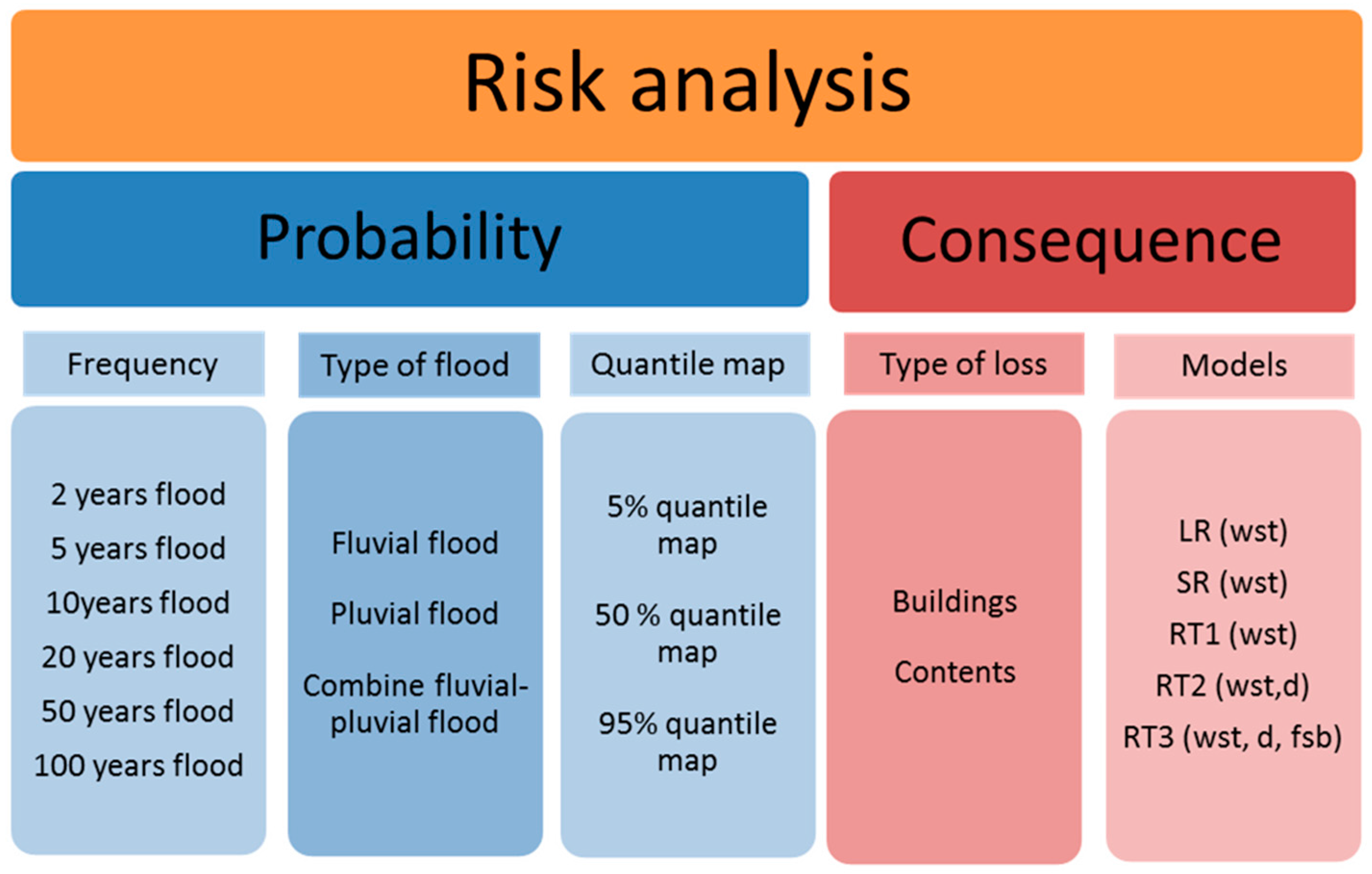
2.3.1. Flood Hazard Scenarios
The water depth values are taken from flood hazard maps simulated by Apel et al. [5] to analyze flood risk (Figure 2). The maps show maximum inundation depths for Can Tho City with median (50%-quantile) maps and associated 5% and 95% quantile maps for each probability level and for fluvial flood, pluvial flood, and combined fluvial–pluvial flood. Maximum inundation depths below 0.02 m are indicated as no inundation. The range of water depth is from 0.02 m to 2 m. For our risk analysis, we increase the threshold for inundation depth from 0.02 to 0.05 m. This is mainly because, according to the interview results, the households with inundation depths below 0.05 m suffered no damage [23]. The water depth for the pluvial flood is normally lower than 0.5 m. The water depth of fluvial flood and the combined fluvial–pluvial flood is lower than 1 m and, in some places, the depth reaches up to 1.5 m. The flood event in 2011 in Can Tho City was very similar to the 0.95 probability scenario in respect to flood extent and water depth.
2.3.2. Flood Duration Map
Due to complex flood characteristics, including tidal influence, floods last for several days to several months in Can Tho city. As computing capacity for probabilistic flood scenario calculation is limited, flood durations could not be calculated by Apel et al. [5]. For this study, we consider duration values of the 2011 flood event for all hazard scenarios.
Based on duration information provided by interviewed households (Figure 3a), a triangulated irregular network (TIN) was created in ArcGIS. Flood duration map is generated from TIN by using Inverse Distance Weighting (IDW) interpolation method (Figure 3b). The values of duration range from 4 to 1040 h (Figure 3b).
2.3.3. Building Map (Exposure)
The German Space Centre (DLR) provided the building map for the urban area in Can Tho city, including Cai Rang district and two thirds of Ninh Kieu district (Figure 4a). The map was digitized in 2010 from high-resolution QuickBird Image data from 22 December 2006 [29].
The map contains information about the base area (perimeter) of all types of houses in the study area. Unfortunately, it lacks information about building use and characteristic of the buildings. To extract residential buildings from this building map, we have used the land use map 2010, provided by the Department of Natural resources and Environment (DONRE) of Can Tho City (Figure 4b). This map displayed 50 types of land use including urban residential land use.
By using the overlay method in ArcGIS, the residential buildings (red color in Figure 4c) were extracted from the building map of DLR and the land use map 2010 by DONRE.
The residential map contains about 23,500 houses in the study areas including both residential houses only and houses with small businesses. The map provides information about the house location and base area of the house. Using this information, the floor space of the buildings was calculated based on the base area of the building.
3. Methods
3.1. Development of Flood Loss Models
In order to find suitable loss models for residential buildings and contents, we develop, validate and compare both depth–damage functions and decision-tree based models. Since the most common loss models are depth–damage functions [9,10], we use these as a sort of benchmark method for model comparison in our study. To investigate the difference resulting from model structures, we also develop a regression tree with water depth as the only input variable and compare it with the depth–damage-functions. Regression tree-based models are an advancement in flood loss modeling, since they can consider more damage determining variables and capture non-linear behavior of the damage process [18,19]. Thus, based on the identification of the most important loss determining variables during flooding in Can Tho City [24], the following models were setup:
- Depth–damage functions are developed by using linear and square root regression methods.Linear function (LR):Square root function (SRR):
- Four regression tree models are developed:Regression tree with one variable—water depth RT1Regression tree with two variables—water depth, duration RT2Regression tree with three variables—water depth, duration, floor space of building RT3:
Regression tree with four variables—water depth, duration, floor space of building, building/content value RT4. For the building loss model, the building value is used as an input variable. For the contents loss model, the contents value is used as an input variable:
The regression tree based models are developed using the Matlab Statistics Toolbox whose algorithms are based on Breiman et al. (1984) [30]. The tree building algorithm recursively subdivides the predictor data space into smaller regions in order to approximate a nonlinear regression structure. The algorithm searches all possible split values of all predictor variables to identify the split which minimizes the error criterion, i.e., the variance of the response variable (e.g., building loss, or contents loss). We set the minimum number of cases in terminal nodes of the trees to 30. The loss prediction for a specific input is the average of the response variable of all the samples of the training dataset that belong to this terminal node.
The empirical data from interviews in Can Tho City in 2011 (n = 858 observations, Table 1) were used to develop and validate the flood loss models. For validation, a leave-one-out cross validation method is applied [19,31] which uses one observation as the testing (validation) sample and the remaining observations as the training sample and loops in total n times over the observed dataset. The performance of the models, i.e., agreement between the predictions and the observed values is quantified by mean bias error (MBE), mean absolute error (MAE), root mean square error (RMSE) and correlation coefficient [31]. MBE indicates the average bias of the model; MAE provides the average absolute deviation of the modeled values from observed values; and RMSE indicates square root of a variance, and correlation coefficient indicates the relationship between model results and observed losses. A positive MBE signifies an overestimation in the modeled values and a negative MBE shows an underestimation.
3.2. Flood Risk Analysis
Flood risk is defined as the relationship between the consequence and its probability [32,33]. Probability is the chance of occurrence of a flood event and in this case, the annual non-exceedance probability of the flood scenarios is considered. The consequence presents the impact of the flood such as economic, social or environmental damage: here, we focus on the direct loss to buildings and contents in monetary values. The risk is generally formulated as the following:
Figure 5 shows the risk analysis components for residential buildings and contents of Can Tho city. In Apel et al. [5], several probabilistic flood hazard maps for Can Tho City were derived for fluvial flood, pluvial flood and combined fluvial–pluvial flood for six return periods: T = 2, 5, 10, 20, 50 and 100 years (p = 0.5; p = 0.8; p = 0.9; p = 0.95; p = 0.98; p = 0.99 respectively). For each probability level, 140 combinations of annual maximum discharge and flood volume and 140 random selections of storm centers were simulated in a Monte Carlo simulation for fluvial flood and pluvial flood, respectively. Then, the combined fluvial and pluvial flood hazard maps were calculated by the 140 fluvial flood scenarios per probability level and adding a synthetic rainstorm event with a random storm center location at the time of the maximum water level of the fluvial scenario boundary. This combination was constructed in the way that the return period of fluvial and pluvial floods is identical (both have the same probability of non-exceedance). The combined floods consider the probability of co-occurrence of the two types of flood (in this study approximately = 0.2). This makes the probability of the occurrence of the combined events to be quite low for all the scenarios.
Because of the natural uncertainty of probabilistic inundation simulation, 5, 50, and 95 percentile flood hazard maps were calculated. The median hazard maps show the expected flood hazard of a given probability of occurrence, and the 5% and 95% percentile maps quantify the uncertainty [5].
The consequence is the potential flood loss for residential buildings and contents in monetary values in prices of the year 2011 in US dollars. Flood losses are calculated by different flood loss models (Equations (1)–(5)) with the input data: water depth maps for each probability level and percentile, duration and floor space of building (see Section 2). Model RT4 (Equation (6)) was not applied for the risk analysis because information on building value and content value are not available.
Expected Annual Damage (EADs)
Expected annual damage (EADs) are defined as the product of the flood damage of the annual probability of exceedance of a given flood event. It can be interpreted as the average annual damage over a very long period of time. According to Apel et al. [5], for a discrete set of scenarios, i.e., probability levels as used in this study, EADs are formulated as the following:
where ΔP is the increment of the probability of exceedance = Δ(1 − p) with p is the probability of non-exceedance, D is the damage inflicted, i is the the numerator of the probability levels considered, and n is the the number of probability levels. Using a linear interpolation, ΔPi and Di are defined as:
Because of the necessary coincidence of fluvial and pluvial floods in the study area, the EADs for the combined fluvial and pluvial flood risk are not the sum of EAD(fl) and EAD(pl) [34]. Instead, the EADs for the combined fluvial and pluvial flood risk is formulated as the following:
4. Results and Discussion
4.1. Flood Loss Models
4.1.1. Depth-Damage Functions
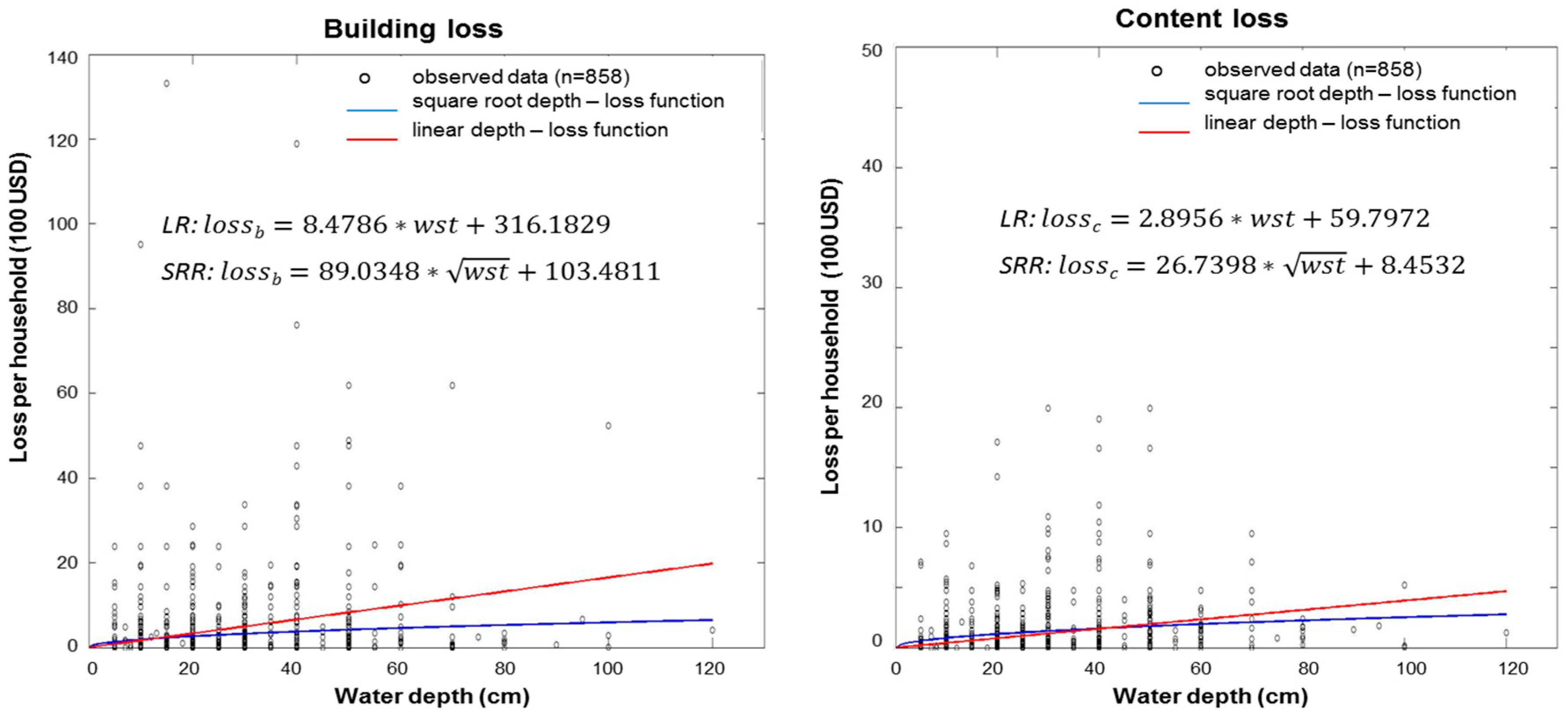
For calculating flood loss to buildings and contents, two different types of absolute water depth–damage functions are developed, namely a linear function and a square root function.
Figure 6 shows the scatter plot between water depth and losses as well as the linear and square root depth–damage functions for building and content damage. The scatter plot shows that the observed building losses are mainly under US$2000 (for 93.2% of the data) and the observed contents losses are mainly under US$500 (for 94.5% of the data).
The linear depth–damage curve for building losses increases slightly, estimating building losses under US$2000 up to a water depth of 120 cm. When the water depth is lower than 60 cm, the building loss is estimated to be below US$1000. Similarly, the linear depth–damage curve for content losses increases slowly, estimating content losses under US$500 up to a water depth of 120 cm. With water depth lower than 60 cm, the content loss is estimated to be below US$250. Thus, according to the linear loss functions, the content loss is estimated to be one-fourth of the building loss.
Figure 6 also presents the square-root water depth–damage functions for building and content loss. The estimated losses slightly increase up to a water depth of 80 cm, above that the estimated losses are nearly stable. Square-root depth–damage functions for building and content loss estimate smaller losses in comparison with the estimates of the linear depth–damage functions, particularly for higher water depths.
4.1.2. Regression Trees with Only Water Depth as Predictor—RT1
RT1 for building loss as well as RT1 for contents loss are developed with only water depth as a predictor investigate the difference resulting from model structures in comparison with the depth–damage functions. Exemplarily, RT1 for building losses is shown in Figure 7. The first split of water depth in RT1 is at 37.5 cm. Among the nodes, the highest water depth is 65 cm, and the lowest water depth node is 9 cm.
4.1.3. Regression Trees with Water Depth and Duration as Predictors—RT2
RT2 for building loss and RT2 for contents loss are developed using inundation duration and water depth as predictors. Exemplarily, RT2 for building loss is shown in Figure 8. The tree is explained by 87% of duration and 13% of water depth. The first split based on duration in RT2 is at 63.5 h. All four nodes in the left part of the tree after the root node split are water depth, which means that, for a shorter duration (d < 63.5 h), the losses are mainly influenced by water depth. In the right part, water depth node split at 37.5 cm, after that there are three nodes of duration.
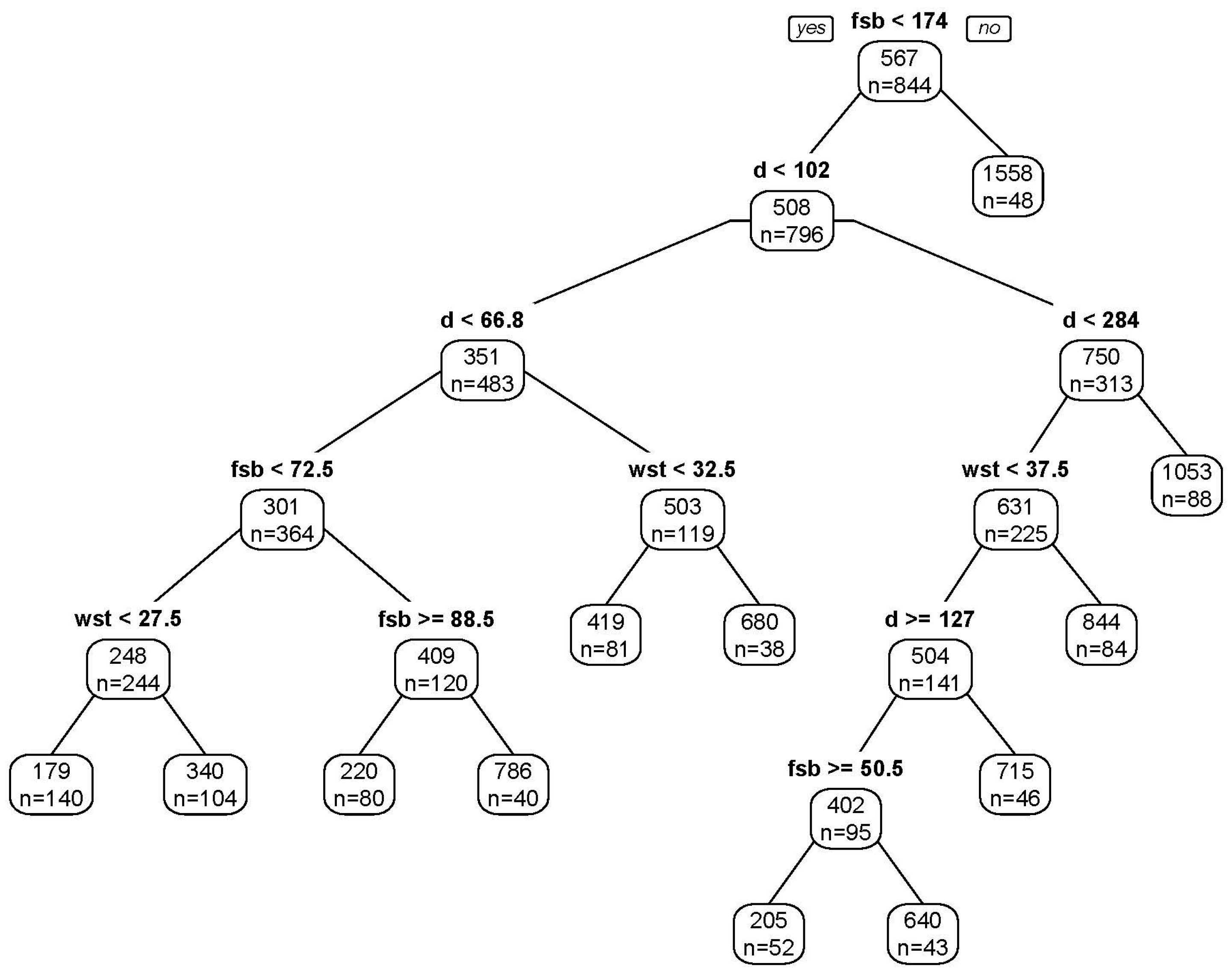
4.1.4. Regression Trees with Water Depth, Duration and Floor Space of Building as Predictors—RT3
RT3 for building loss as well as RT3 for contents loss are developed with water depth (wst), duration (d) and floor space of building (fsb) as predictors. RT3 for buildings loss is exemplarily shown in Figure 9. The relative importance of each predictor is 50%, 35% and 15% for the duration, floor space of building and water depth, respectively. The root split of the tree is floor space of building at 174 m2. The buildings with larger floor space are estimated to have a constant flood loss. There are only 48 buildings in this floor space class. The second node split by duration is at 102 h. The largest water depth split is at 37.5 cm.
4.1.5. Regression Trees with Water Depth, Duration, Floor Space of Building and Building/Contents Value as Predictors—RT4
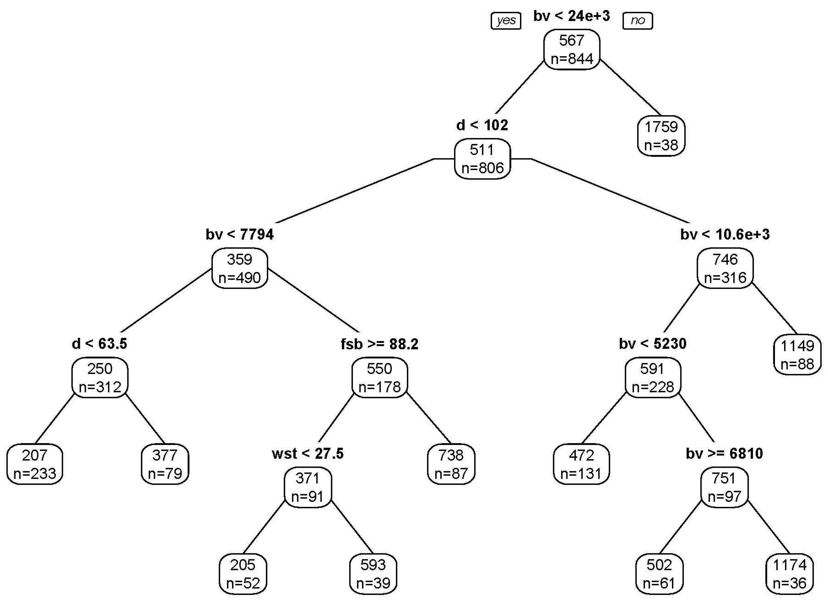
RT4 for building loss is developed with water depth, duration, floor space of building and building value as predictors. RT4 for contents loss is developed similarly with water depth, duration, floor space of building and contents value as predictors. RT4 for building loss is exemplarily shown in Figure 10. The root split of the RT4 tree is building value at US$24 thousand. The buildings with larger values are estimated to have a constant flood loss. There are 38 buildings in this building value class. The second node splits by duration at 102 h. For longer duration (d > 102 h), only building value is important for estimating building loss. Water depth has only a small contribution in this tree as there is only one water depth node at 27.5 cm.
4.1.6. Comparison of Model Performance
The leave-one-out cross-validation method described in Section 3.1 is used to compare the performance of the loss models.
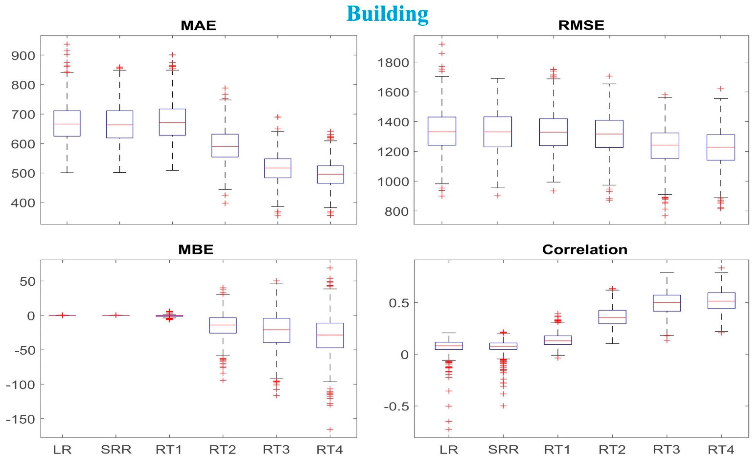
The performance measures of the building loss models (Figure 11) show that the multi-variable loss models, namely RT2, RT3, and RT4, perform better in comparison with the depth–damage functions and RT1. An exception is MBE: the multi-variable models tend to underestimate the loss, which is not the case for the one-variable models. Mean absolute errors range US$500–650. Mean bias errors range US$0–25. In respect to MAE, RMSE, and correlation, RT3 and RT4 perform better than RT2. RT4 has the best performance among all models. However, there is only a small improvement between RT3 and RT4.
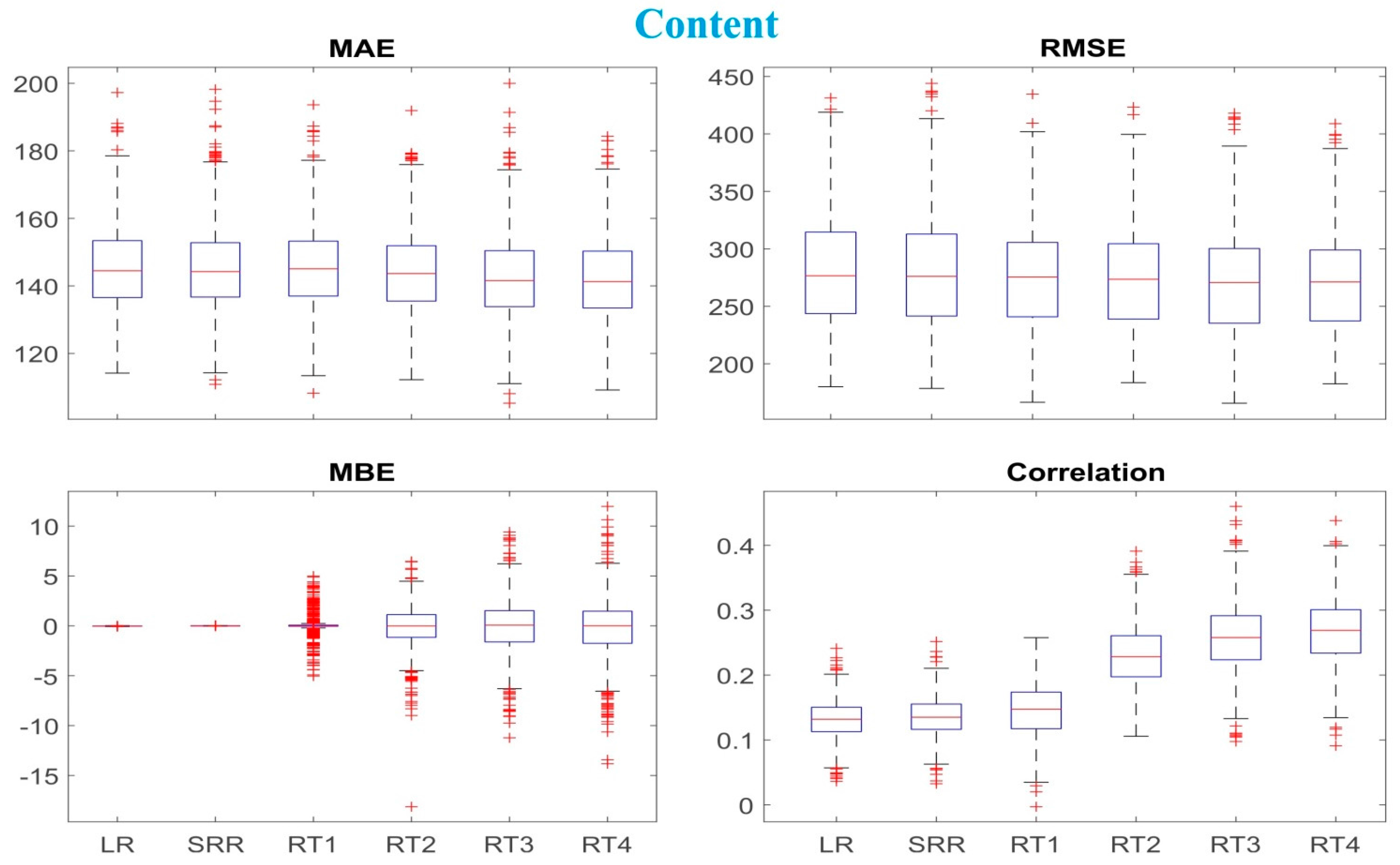
For content loss, all models have similar performance in respect to MAE, MBE, and RMSE (Figure 12). However, correlation coefficients of the multi-variable models are clearly better in comparison with the one-variable models. RT3 and RT4 have the highest correlation coefficients, but between RT3 and RT4, correlation coefficients are not much different.
For one-variable building and contents loss models, there is hardly a difference in performance due to model structure. Linear and square-root water depth–damage functions, as well as RT1, show the same or at least very similar performance. Differences in loss models are apparently due to the amount and selection of predictors. This is in accordance with previous studies, which revealed a significant improvement of flood loss modeling when using multivariable models (e.g., Zhai et al., 2005 [35]; Seifert et al., 2010 [31]; and Merz et al., 2013 [18]). However, one needs to avoid overfitting. Models using (too) many predictors may agree well with the training data, but their prediction ability for independent data is poor. Additionally, more input parameters also introduce additional uncertainty. Thus, when looking for the “best” loss model, one actually looks for a loss model with the best performance and the smallest number of variables (principle of parsimony). Thus, in our study, RT3 seems to be the best model for estimating building loss. For contents loss, RT3 appears most suitable as well, however, since the depth–damage functions perform similarly well, they should be selected due to the principle of parsimony. However, in our flood risk analysis, we applied an ensemble approach to all developed loss models, except RT4 (due to a lack of input data).
4.2. Flood Risk Analysis
The flood risk analysis results in flood risk curves and expected annual damage (EADs) for building and content loss due to fluvial, pluvial and combined fluvial–pluvial floods. The flood risk curves represent damage for building and content of return periods of 2, 5, 10, 20, 50 and 100 years of flood hazards. Expected annual damages represent the average damage over 100 years period.
Both flood risk curves and expected annual damages are calculated for 5%, median (50%) and high 95% quantile maps.
4.2.1. Risk Curves
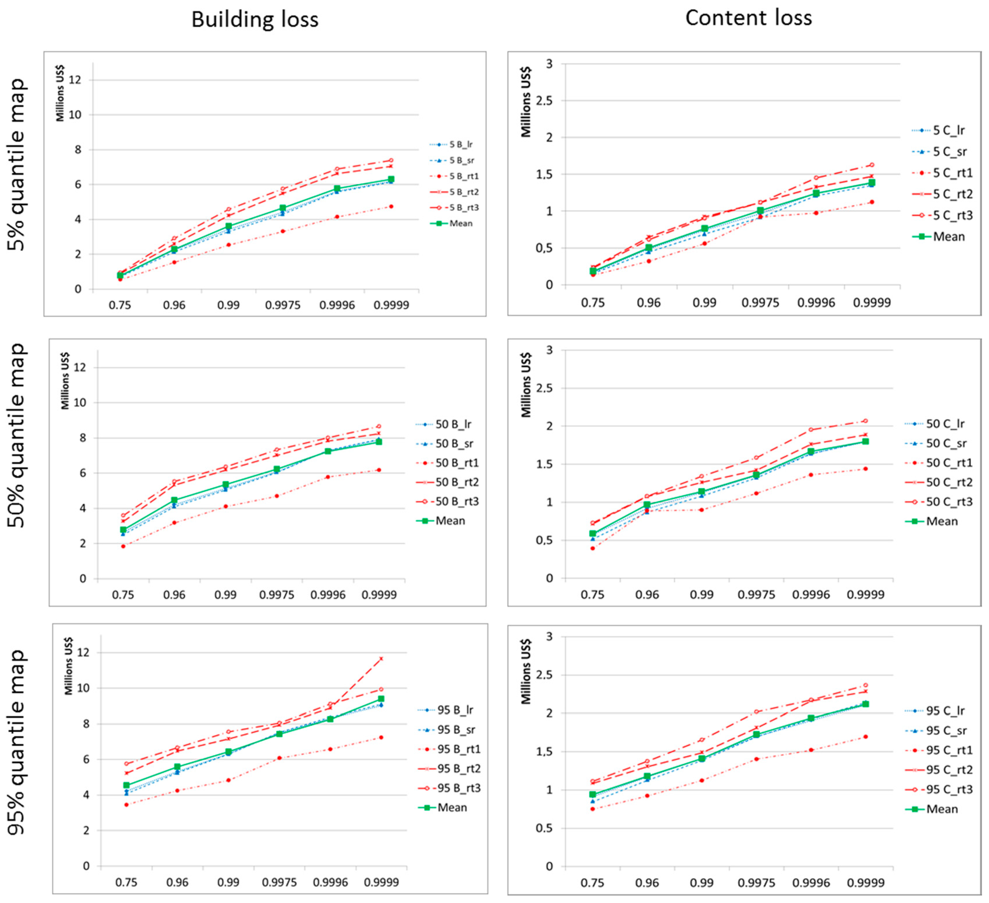
The risk curves for fluvial, pluvial and combined fluvial–pluvial flood hazard and building and content are represented in Figure 13, Figure 14 and Figure 15. For all scenarios and methods, the curve of the mean of building risk and content risk are closest to the linear regression curves. The risk curve of RT1 is lowest, both risk curves resulting from depth–damage functions are in the middle, while risk curves from RT2 and RT3 are highest.
Figure 13 shows risk curves for different fluvial flood scenarios and building and content losses. The results indicate that there is a sharp increase of losses with increased probability in all low (5%), median (50%) and high (95%) quantile maps. For the low quantile map at 0.5 probability level, loss results are nearly the same for all models (the range is US$0.4–0.6 million for building loss, and US$0.1–0.2 million for content loss). At 0.99 probability level, the ranges reach up to US$4–6 million for building loss and up to US$1–1.4 million for content loss. This is about 10 times larger than losses at 0.5 probability level. In the median quantile map, the range of losses for the building is US$1–2 million at 0.5 probability level. However, at 0.99 probability level, the loss range is US$6–8.4 million. This is about five times higher than at the 0.5 probability level. In the high quantile map, the range of losses for the building is US$1.5–2.8 million at 0.5 probability level, and US$7.2–11.6 million at 0.99 probability level. The risk curve for building loss with RT2 at 0.99 probability level estimates surprisingly high losses, which is due to many buildings being exposed to water depth larger than 37.5 cm and durations longer than 246 h.
The risk curves for pluvial flood scenarios are shown in Figure 14. The curves increase slightly by about 50% from 0.5 to 0.99 probability level in high quantile map. The risk curves increase considerably, from nearly no losses at 0.5 probability level to US$3–5 million at 0.99 probability level for 5% quantile map. In the median quantile map, the risk curves increase from a range US$0.7–1.7 million at 0.5 probability to a range US$2.7–5 million at 0.99 probability level. It reflects that small rainfall causes no damage, whereas a large amount of rainfall causes significant damage up to a certain threshold, and then losses increase very slowly.
Figure 15 shows the risk curves of combined pluvial–fluvial flood scenarios and building and content losses. The trend of these curves is similar to risk curves of the fluvial flood. The influence of pluvial flood is apparent at probability 0.75 in the 95% quantile map. The curves start at range US$3.5–5.8 million, which is higher than the curves of fluvial flood scenarios with probability 0.5 and 95% quantile map (range US$1.5–2.8 million).
The median quantile maps represent the expected flood risk at a given probability of occurrence, while the 5% and 95% quantile maps quantify the uncertainty. In order to evaluate the uncertainty in risk curves due to the hazard uncertainty, we calculate the mean absolute difference of risk estimation between the 5%/95% and the 50% quantile maps in the percentage of all models and for each probability level (Table 2). In order to evaluate the uncertainty in risk curves due to the flood loss modeling, we calculate the mean absolute difference in the percentage of risk estimation between the min/max loss values and mean loss value of all models and median quantile maps for each probability (Table 2).
Due to uncertainties in the hazard calculations, the lower is the annual non-exceedance probability, the higher is the uncertainty of the flood risk estimation (Table 2). The results of pluvial flood hazard maps show a large uncertainty of risk (mean absolute differences range is 17–110% for building loss and 19–111% for content loss), particularly for 0.5 annual non-exceedance probability. However, the uncertainty is reduced at high probability levels (mean absolute differences range is 12–20% for 0.99 annual non-exceedance probability).
The uncertainty of flood risk due to uncertainties in the flood loss modeling for the building is quite similar to type of floods and annual non-exceedance probabilities (mean absolute differences range is 10–20% for building loss and 8–15% for content loss). Uncertainty due to hazard modeling is about three times higher than uncertainty due to damage modeling.
4.2.2. Expected Annual Damage (EADs)
The expected annual damage (EADs) for fluvial flood hazard, pluvial flood hazard, and combined pluvial–fluvial flood hazard are estimated by using Equations (7) and (10). The results are shown in Table 3, Table 4 and Table 5.
Generally, EADs from fluvial flood hazards are always higher than expected annual damages from pluvial flood hazard. On average, the building losses are approximately US$1556 thousand for fluvial and US$1230 thousand for pluvial floods. The annual expected content loss is about 20% of annual expected building loss: it is about US$347 thousand for fluvial and US$261 thousand for pluvial flood hazard. Total expected annual loss for all private households in the study area, i.e., sum of EAD of building and content, is US$1903 thousand for fluvial flood hazard; US$1490 thousand for pluvial flood hazard; and US$3340 thousand for combined fluvial–pluvial flood hazard. EADs estimation by model RT3 always provides the highest value, whereas RT1 provides the lowest value in comparison with other models. Mean absolute differences of EADs of total losses due to hazard uncertainty for fluvial flood hazard is on average 40%, for pluvial flood hazard is on average 71% and for combined fluvial–pluvial flood hazard is on average 52% (Table 3, Table 4 and Table 5). Mean absolute differences of EADs due to loss model uncertainty for fluvial flood hazard is on average 22%, for pluvial flood hazard is on average 39% and for combined fluvial–pluvial flood hazard is on average 26%. Thus, uncertainty due to hazard modeling is nearly double as high as uncertainty due to damage modeling. The combined uncertainty due to hazard and damage modeling ranges between an average of 60% for fluvial floods and 112% for pluvial floods.
Because the study area is affected by both fluvial and pluvial floods occurring at the same time of the year, the most realistic EADs for private households in the study area is the one calculated for combined fluvial–pluvial floods (Table 5), i.e., US$3340 thousand of total loss per year. This is approximately 2.5% of total annual income of households in the study area (according to Vo, T.D., 2014 [21] the mean annual income of a household is US$5792 and there are 23,500 houses located in the study area).
5. Conclusions
The development and validation of loss models for private households in Can Tho City reveal that multi-variable models outperform depth–damage functions, especially for residential building loss. Damage processes due to the specific flood characteristics in the Mekong delta, where inundation duration and building characteristics are more important than water depth for determining the resulting loss [21], can be better described by loss models which consider some of these variables. The regression tree based loss model RT3 with the three predictors water depth, inundation duration and floor space of the building is recommended for building loss estimation, since it represents the best compromise between model performance and model complexity. For contents loss estimation the model performances for both RT3 and depth–damage functions are similar. In the flood risk analysis, we applied an ensemble approach using two depth–damage functions and three decision-tree based loss models, to capture uncertainty due to loss modeling.
Building value is considered as an important parameter for flood damage modeling [24]. However, systematic data for building value are not available in many parts of the developing world. Our analysis for Can Tho City suggests that damage estimation with three parameters (water depth, inundation duration and floor space of building) is valid even without considering building value as additional model input.
The risk analysis for the inner city of Can Tho reveals the risk curves and expected annual damage for fluvial, pluvial and combined fluvial–pluvial floods. The uncertainty of risk estimates is high. The average mean difference in EADs for combined fluvial–pluvial floods for total loss reaches 79%. Uncertainty due to hazard modeling is nearly twice as high as uncertainty due to damage modeling. This shows, on the one hand, the high importance of uncertainty quantification by means of probabilistic or ensemble approaches, and, on the other hand, stresses the need for more research to better understand risk processes in complex situations such as the Mekong Delta as well as for improved models and approaches.
The expected annual damage to residential buildings and contents for the inner urban area of Can Tho City is about US$3340 thousand, which is about 2.5% of the total annual income of all households in the study area. This is a quite large fraction, stressing the importance of improving flood risk management in the Mekong Delta. Risk analyses are essential for decision makers in planning efficient flood risk management.
Acknowledgments
This research was carried out as part of the “Water related Information System for a Sustainable development of the Mekong Delta” (WISDOM II) project. Funding by the German Ministry of Education and Research (BMBF) and the Vietnamese Ministry of Science and Technology (MOST) is gratefully acknowledged. AK Gain is financially supported by the Alexander von Humboldt Foundation whose support is gratefully acknowledged.
Author Contributions
Do Thi Chinh and Heidi Kreibich developed the concept of this study. The analysis was carried out by Do Thi Chinh and Nguyen Viet Dung. Do Thi Chinh drafted the first version of the article, all authors worked on improving and finalizing the article.
Conflicts of Interest
The authors declare no conflict of interest.
References
- Gain, A.K.; Mojtahed, V.; Biscaro, C.; Balbi, S.; Giupponi, C. An integrated approach of flood risk assessment in the eastern part of Dhaka city. Nat. Hazards 2015, 79, 1499–1530. [Google Scholar] [CrossRef]
- Oanh, L.N.; Thuy, N.T.T.; Widerspin, I.; Coulier, M. A Preliminary Analysis of Flood and Storm Disaster Data in Vietnam; UNDP: New York, NY, USA; ISDR: Los Angeles, CA, USA, 2011. [Google Scholar]
- The World Bank (WB). Weathering the Storm: Options for Disaster Risk Financing in Vietnam; The World Bank: Washington, WA, USA, 2010. [Google Scholar]
- Hung, N.N.; Degado, J.M.; Tri, V.K.; Apel, H. Floodplain hydrology of the Mekong delta, Vietnam. Hydrol. Processes 2012, 26, 674–686. [Google Scholar] [CrossRef]
- Apel, H.; Martínez Trepat, O.; Hung, N.N.; Chinh, D.T.; Merz, B.; Dung, N.V. Combined fluvial and pluvial urban flood hazard analysis: Concept development and application to can tho city, Mekong delta, Vietnam. Nat. Hazards Earth Syst. Sci. 2016, 16, 941–961. [Google Scholar] [CrossRef]
- Southern Institute of Water Resources Research (SIWRR). Development of Cantho City and Resilient Project—Hydraulic Report; Southern Institute of Water Resources Research: Ho Chi Minh City, Vietnam, 2016. [Google Scholar]
- Can Tho Committee for Flood and Storm Control (CCFSC). Annual Disaster Report; Can Tho Committee for Flood and Storm Control: Can Tho City, Vietnam, 2011. [Google Scholar]
- De Moel, H.; Jongman, B.; Kreibich, H.; Merz, B.; Penning-Rowsell, E.; Ward, P.J. Flood risk assessments at different spatial scales. Mitig. Adapt. Strateg. Glob. Chang. 2015, 20, 865–890. [Google Scholar] [CrossRef]
- Gerl, T.; Kreibich, H.; Franco, G.; Marechal, D.; Schroter, K. A review of flood loss models as basis for harmonization and benchmarking. PLoS ONE 2016, 11, e0159791. [Google Scholar] [CrossRef] [PubMed]
- Merz, B.; Kreibich, H.; Schwarze, R.; Thieken, A. Review article ‘assessment of economic flood damage’. Nat. Hazards Earth Syst. Sci. 2010, 10, 1697–1724. [Google Scholar] [CrossRef]
- Thieken, A.H.; Muller, M.; Kreibich, H.; Merz, B. Flood damage and influencing factors: New insights from the August 2002 flood in Germany. Water Resour. Res. 2005, 41. [Google Scholar] [CrossRef]
- Smith, D. Flood damage estimation—A review of urban stage-damage curve and loss functions. Water SA 1994, 20, 231–238. [Google Scholar]
- US Army Corps of Engineers (USACE). Risk-based analysis for flood damage reduction studies. In Proceedings of the 1997 Hydrology & Hydraulics Workshop, Pacific Grove, CA, USA, 20–22 October 1997; US Army Corps of Engineers: Washington, WA, USA, 1997. [Google Scholar]
- Pistrika, A. Flood damage estimation based on flood simulation scenarios and a GIS platform. Eur. Water 2010, 30, 3–11. [Google Scholar]
- Merz, B.; Kreibich, H.; Thieken, A.; Schmidtke, R. Estimation uncertainty of direct monetary flood damage to buildings. Nat. Hazards Earth Syst. Sci. 2004, 4, 153–163. [Google Scholar] [CrossRef]
- Penning-Rowsell, E.C. The Benifits of Flood and Coastal Risk Management: A Handbook of Assessment Techniques; Middlesex Unversity Press: London, UK, 2005. [Google Scholar]
- Dutta, D. Direct Flood Damage Modeling towards Urban Flood Risk Management; International Center for Urban Safety Engineering (ICUS/INCEDE), IIS, The University of Tokyo: Tokyo, Japan, 2001. [Google Scholar]
- Merz, B.; Kreibich, H.; Lall, U. Multi-variate flood damage assessment: A tree-based data-mining approach. Nat. Hazards Earth Syst. Sci. 2013, 13, 53–64. [Google Scholar] [CrossRef]
- Kreibich, H.; Botto, A.; Merz, B.; Schröter, K. Probabilistic, multivariable flood loss modeling on the mesoscale with BT-FLEMO. Risk Anal. 2016. [CrossRef] [PubMed]
- Mekong River Commission (MRC). Flood Damages, Benefits and Flood Risk in Focal Areas; Mekong River Commission: Vientiane, Laos, 2009. [Google Scholar]
- Vo, T.D. Household Economic Losses of Urban Flooding—Case Study of Can Tho City; Vietnam; International Institute for Environment and Development: London, UK, 2014. [Google Scholar]
- Vu, T.T.; Ranzi, R. Flood risk assessment and coping capacity of floods in Central Vietnam. J. Hydro-Environ. Res. 2017, 14, 44–60. [Google Scholar] [CrossRef]
- Chinh, D.T.; Bubeck, P.; Dung, N.V.; Kreibich, H. The 2011 flood event in the Mekong delta: Preparedness, response, damage, and recovery of private households and small businesses. Disaster 2016, 40, 753–778. [Google Scholar] [CrossRef] [PubMed]
- Chinh, D.T.; Gain, A.; Dung, N.V.; Haase, D.; Kreibich, H. Multi-variate analyses of flood loss in Can Tho city, Mekong delta. Water 2015, 8, 6. [Google Scholar] [CrossRef]
- Can Tho City People Committee. Can Tho City Statistic; Can Tho City People Committee: Can Tho City, Vietnam, 2011.
- Huu, P.C. Planning and Implementation of the Dyke Systems in the Mekong Delta, Vietnam. Ph.D. Thesis, Rheinischen Friedrich-Wilhelms University of Bonn, Bonn, Germany, 2011. [Google Scholar]
- Can Tho City People’s Committee. Can Tho City Climate Change Resilience Plan, 2010; Can Tho City People’s Committee: Can Tho City, Vietnam, 2010.
- Southern Institute for Water Resources Planning (SIWRP). Flood Prevention Planning for Can Tho City; Southern Institute for Water Resources Planning: Ho Chi Minh City, Vietnam, 2010. [Google Scholar]
- Water-Related Information System for the Sustainable Development of the Mekong Delta (WISDOM). Vietnam—Can Tho City—Land Use/Land Cover 2006; German Aerospace Center (DLR): Köln, Germany, 2010. [Google Scholar]
- Breiman, L.; Friedman, J.; Olshen, R.A.; Stone, C.J. Classification and Regression Trees; Wadsworth: Belmont, CA, USA, 1984. [Google Scholar]
- Seifert, I.; Kreibich, H.; Merz, B.; Thieken, A.H. Application and validation of FLEMOcs—A flood-loss estimation model for the commercial sector. Hydrol. Sci. J. 2010, 55, 1315–1324. [Google Scholar] [CrossRef]
- The Federal Emergency Management Agency (FEMA). Guidance for Flood Risk Analysis and Mapping First Order Approximation; The Federal Emergency Management Agency (FEMA): Washington, WA, USA, 2015.
- Floodsite. Language of Risk: Project Definitions; HR Wallingford: Wallingford, UK, 2009. [Google Scholar]
- Dasgupta, S.; Laplante, B.; Meisner, C.; Wheeler, D.; Yan, J. The Impact of Sea Level Rise on Developing Countries: A Comparative Analysis; World Bank: Washington, WA, USA, 2007. [Google Scholar]
- Zhai, G.; Fukuzono, T.; Ikeda, S. Modelling flood damage: Case of Tokai flood 2000. J. Am. Water Resour. Assoc. 2005, 41, 77–92. [Google Scholar] [CrossRef]
Figure 1.
Study area in Can Tho city, red points indicate where interviews with private households were undertaken. The inundation map indicates in blue color the flood water depth during the 2011 flood. The inundation was simulated for the study area only, not for the whole of Can Tho city.
Figure 1.
Study area in Can Tho city, red points indicate where interviews with private households were undertaken. The inundation map indicates in blue color the flood water depth during the 2011 flood. The inundation was simulated for the study area only, not for the whole of Can Tho city.
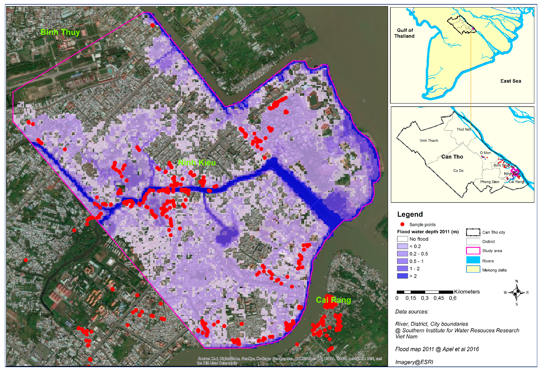
Figure 2.
Derived probabilistic: fluvial flood (a); pluvial flood (b); and combined fluvial–pluvial (c) flood hazard maps [5].
Figure 2.
Derived probabilistic: fluvial flood (a); pluvial flood (b); and combined fluvial–pluvial (c) flood hazard maps [5].
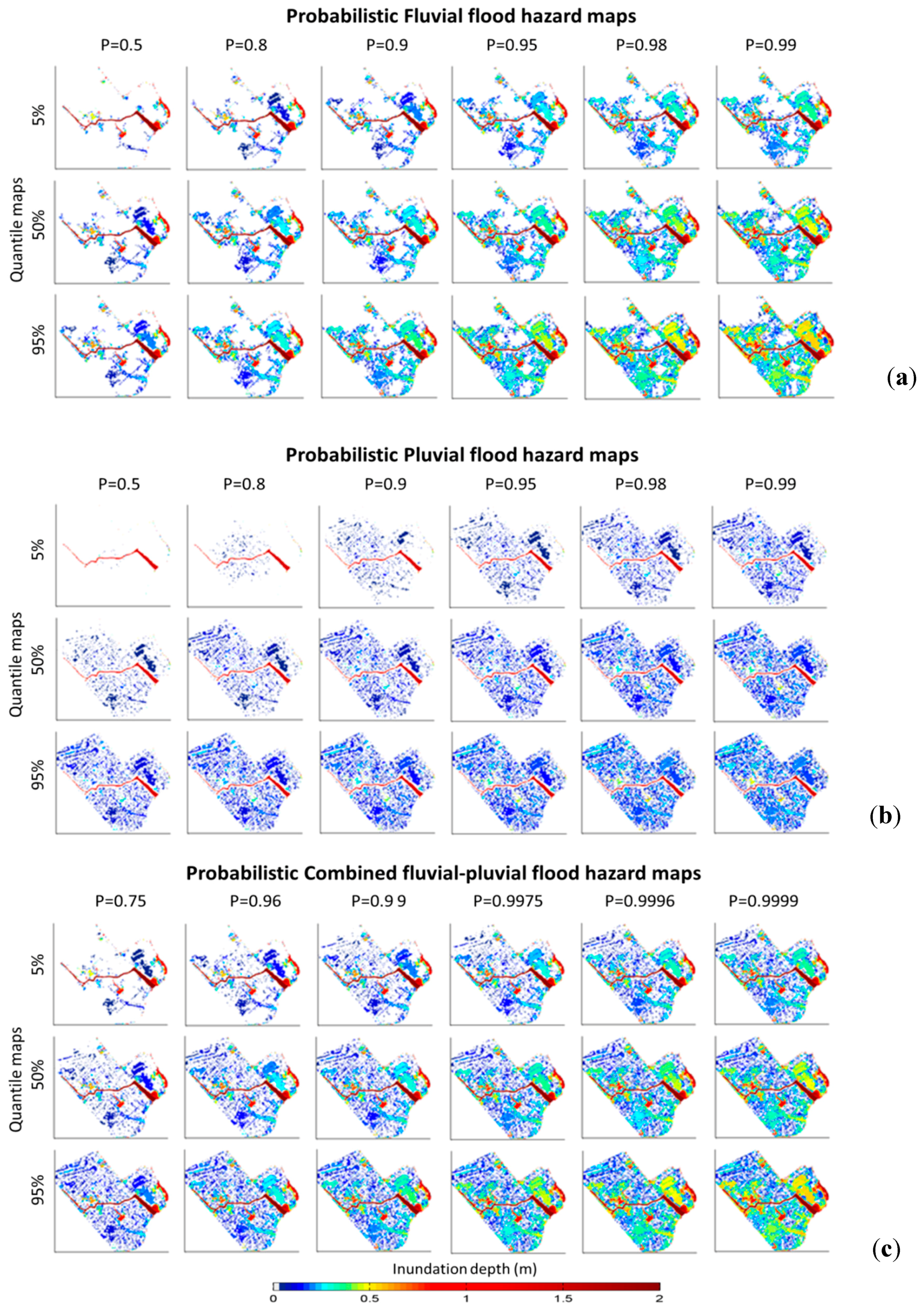
Figure 3.
Flood duration map (b) made based on the inundation duration information provided by interviewed households (a).
Figure 3.
Flood duration map (b) made based on the inundation duration information provided by interviewed households (a).
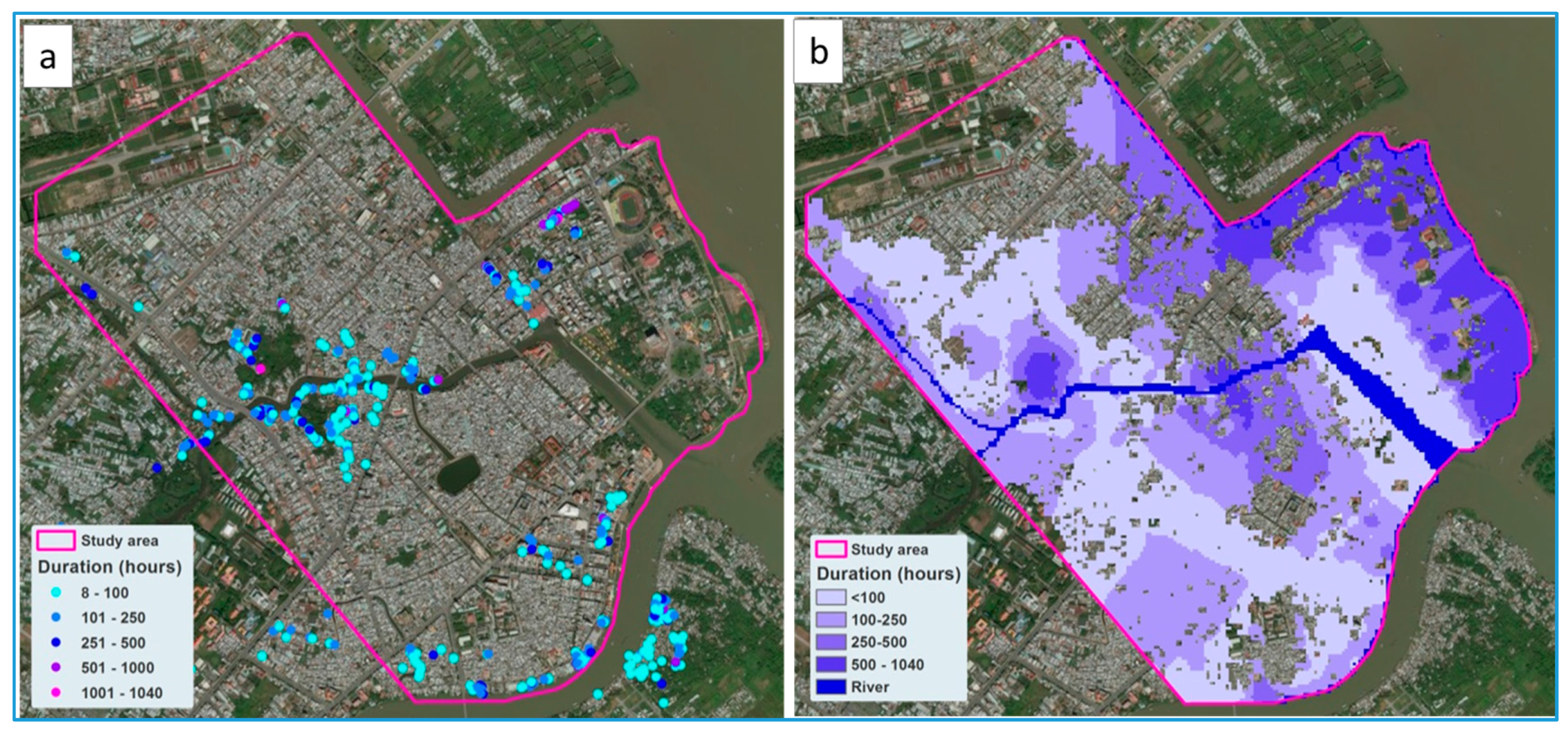
Figure 4.
Study area: building map for the inner city of Can Tho [29] (a); land use map 2010 of Can Tho City by DONRE (b); and developed residential building map for the study area (c) based on the maps in (a,b).
Figure 4.
Study area: building map for the inner city of Can Tho [29] (a); land use map 2010 of Can Tho City by DONRE (b); and developed residential building map for the study area (c) based on the maps in (a,b).
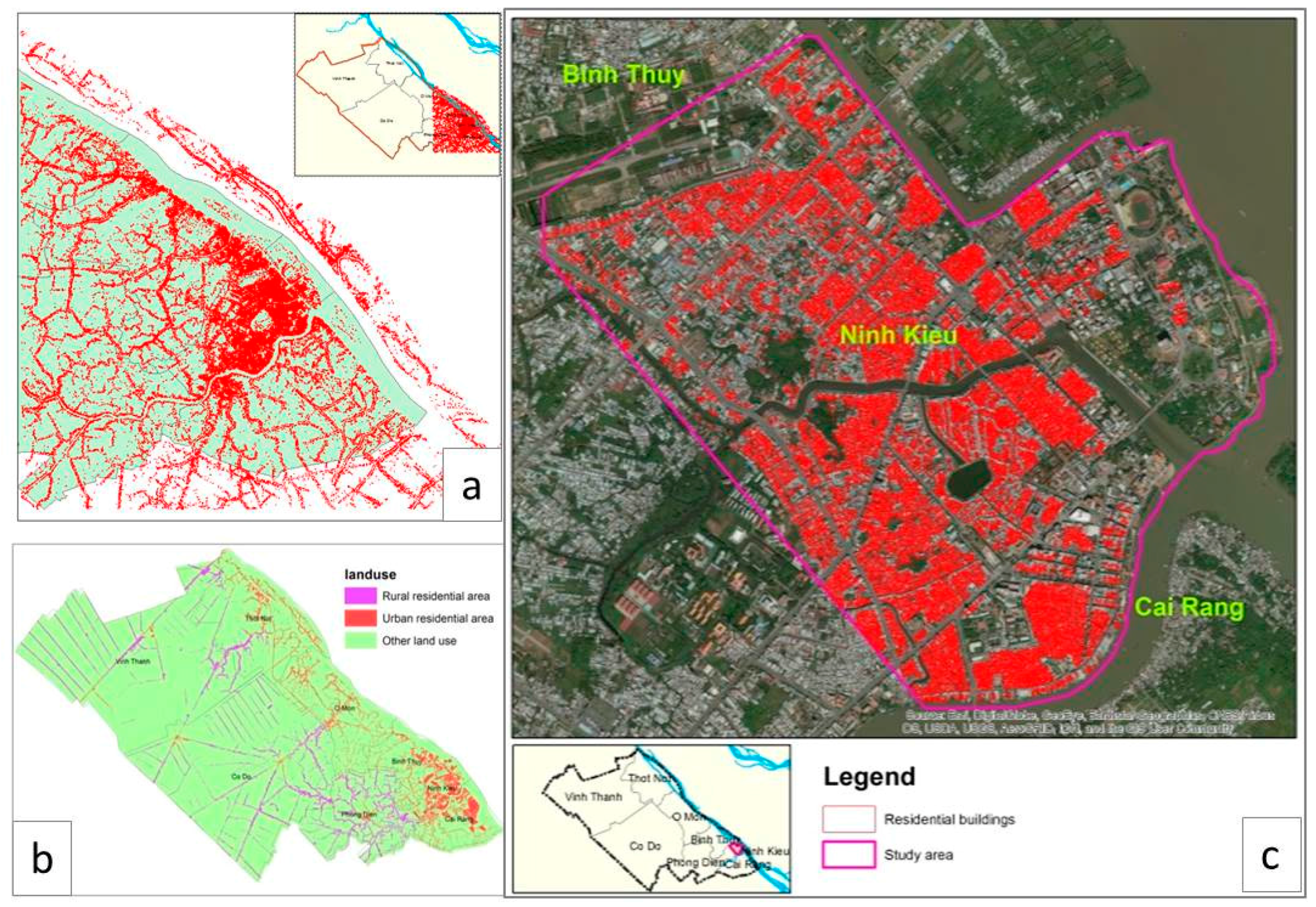
Figure 5.
Risk analysis components for residential buildings and contents of Can Tho city.

Figure 6.
Absolute water depth–damage square root (SRR) and linear (LR) functions for building and contents loss.
Figure 6.
Absolute water depth–damage square root (SRR) and linear (LR) functions for building and contents loss.

Figure 7.
Regression tree with nine leaves for estimating building loss with water depth (wst) as a predictor (RT1). The left part of the tree indicates the “yes” of the clause at nodes, while the right part of the tree indicates the “no” of the clause at nodes.
Figure 7.
Regression tree with nine leaves for estimating building loss with water depth (wst) as a predictor (RT1). The left part of the tree indicates the “yes” of the clause at nodes, while the right part of the tree indicates the “no” of the clause at nodes.
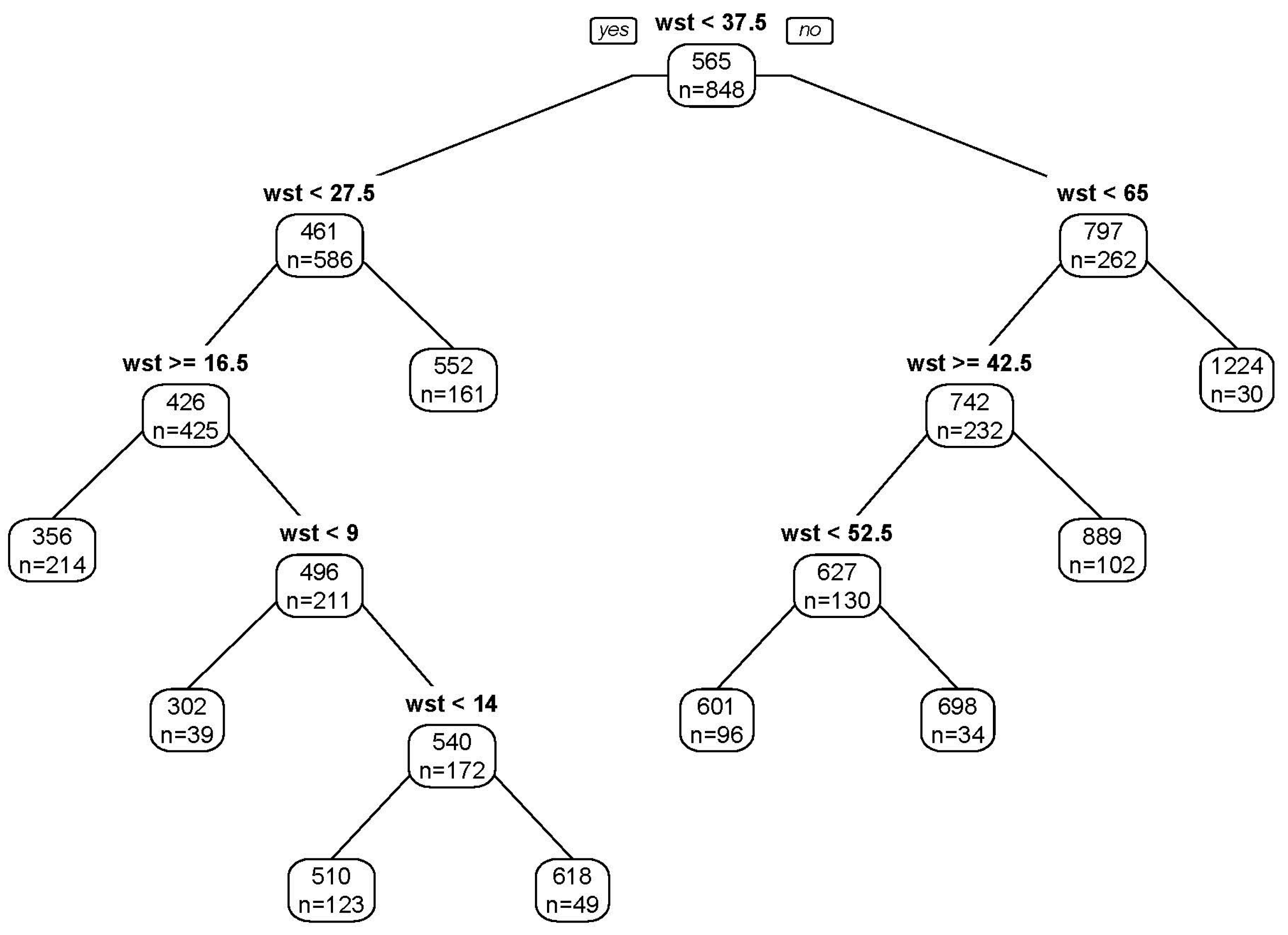
Figure 8.
Regression tree with 11 leaves for estimating building loss with water depth (wst) and duration (d) as predictors (RT2). The left part of the tree indicates the “yes” of the clause at nodes, while the right part of the tree indicates the “no” of the clause at nodes.
Figure 8.
Regression tree with 11 leaves for estimating building loss with water depth (wst) and duration (d) as predictors (RT2). The left part of the tree indicates the “yes” of the clause at nodes, while the right part of the tree indicates the “no” of the clause at nodes.
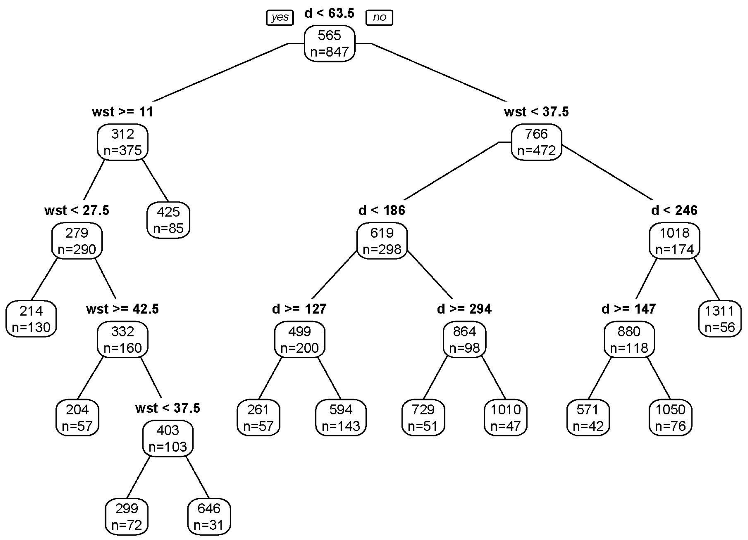
Figure 9.
Regression tree with 11 leaves for estimating building loss using water depth (wst), duration (d) and floor space of building (fsb) as predictors (RT3). The left part of the tree indicates the “yes” of the clause at nodes, while the right part of the tree indicates the “no” of the clause at nodes.

Figure 10.
Regression tree with nine leaves for estimating building loss using water depth (wst), duration (d), floor space of building (fsb) and building value (bv) as predictors (RT4). The left part of the tree indicates the “yes” of the clause at nodes, while the right part of the tree indicates the “no” of the clause at nodes.

Figure 11.
Performance measures: errors and correlation coefficient of building loss models. The boxplots indicate the mean absolute error (MAE), root-mean square error (RMSE), mean bias (MBE), and the correlation coefficient of the models.
Figure 11.
Performance measures: errors and correlation coefficient of building loss models. The boxplots indicate the mean absolute error (MAE), root-mean square error (RMSE), mean bias (MBE), and the correlation coefficient of the models.

Figure 12.
Performance measures: errors and correlation coefficient of content loss models. The boxplots indicate the mean absolute error (MAE), root-mean square error (RMSE), mean bias (MBE), and the correlation coefficient of the models.
Figure 12.
Performance measures: errors and correlation coefficient of content loss models. The boxplots indicate the mean absolute error (MAE), root-mean square error (RMSE), mean bias (MBE), and the correlation coefficient of the models.

Figure 13.
Risk curves for different fluvial flood scenarios and building and content losses. The blue lines indicate the linear and square root depth–damage functions. The red lines indicate the tree-base models with different numbers of predictors. The green line indicates the mean value of all models.
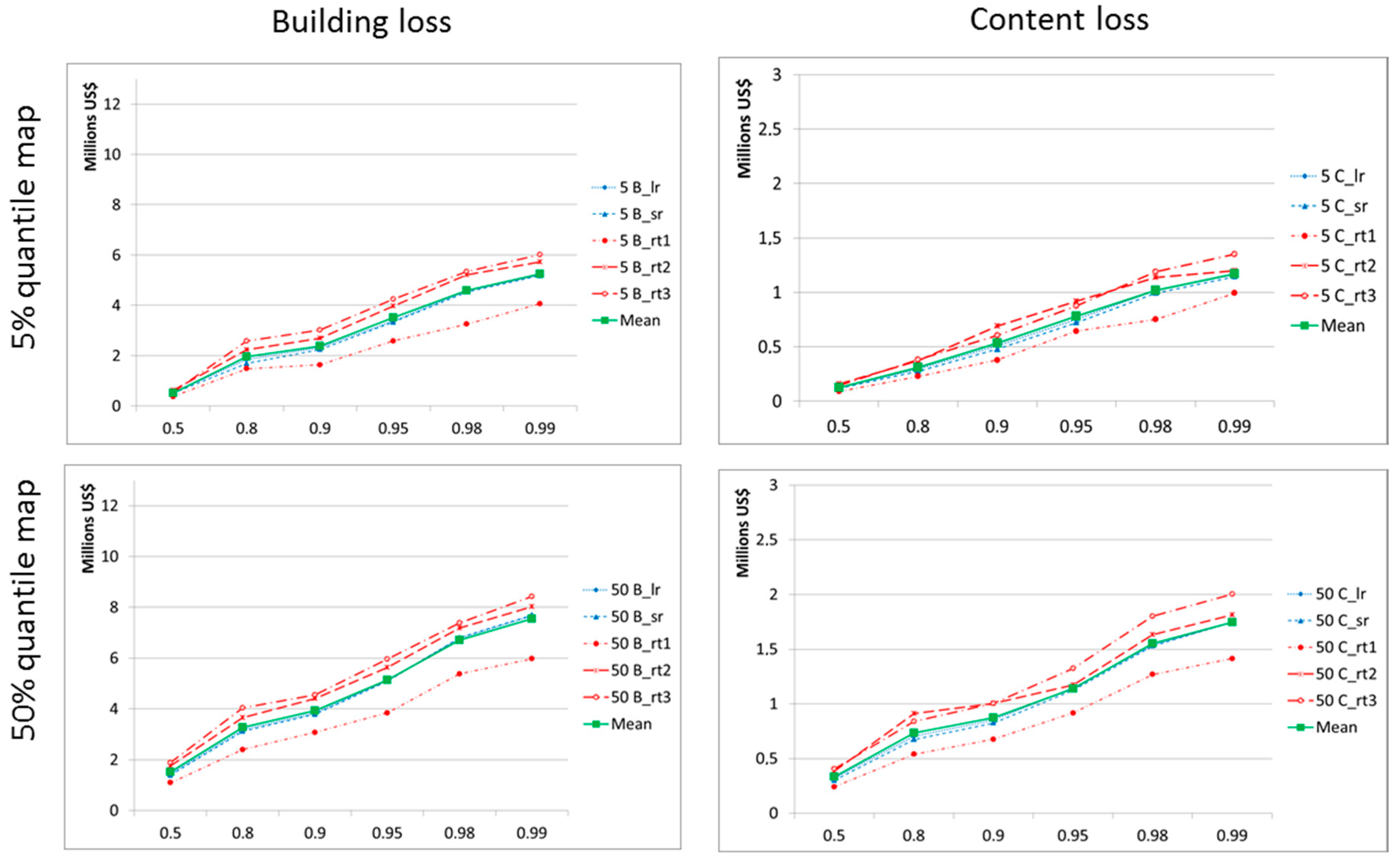

Figure 14.
Risk curves for different pluvial flood scenarios and building and content losses. The blue lines indicate the linear and square root water depth–damage functions. The red lines indicate the tree-base models with different numbers of predictors. The green line indicates the mean value of all models.
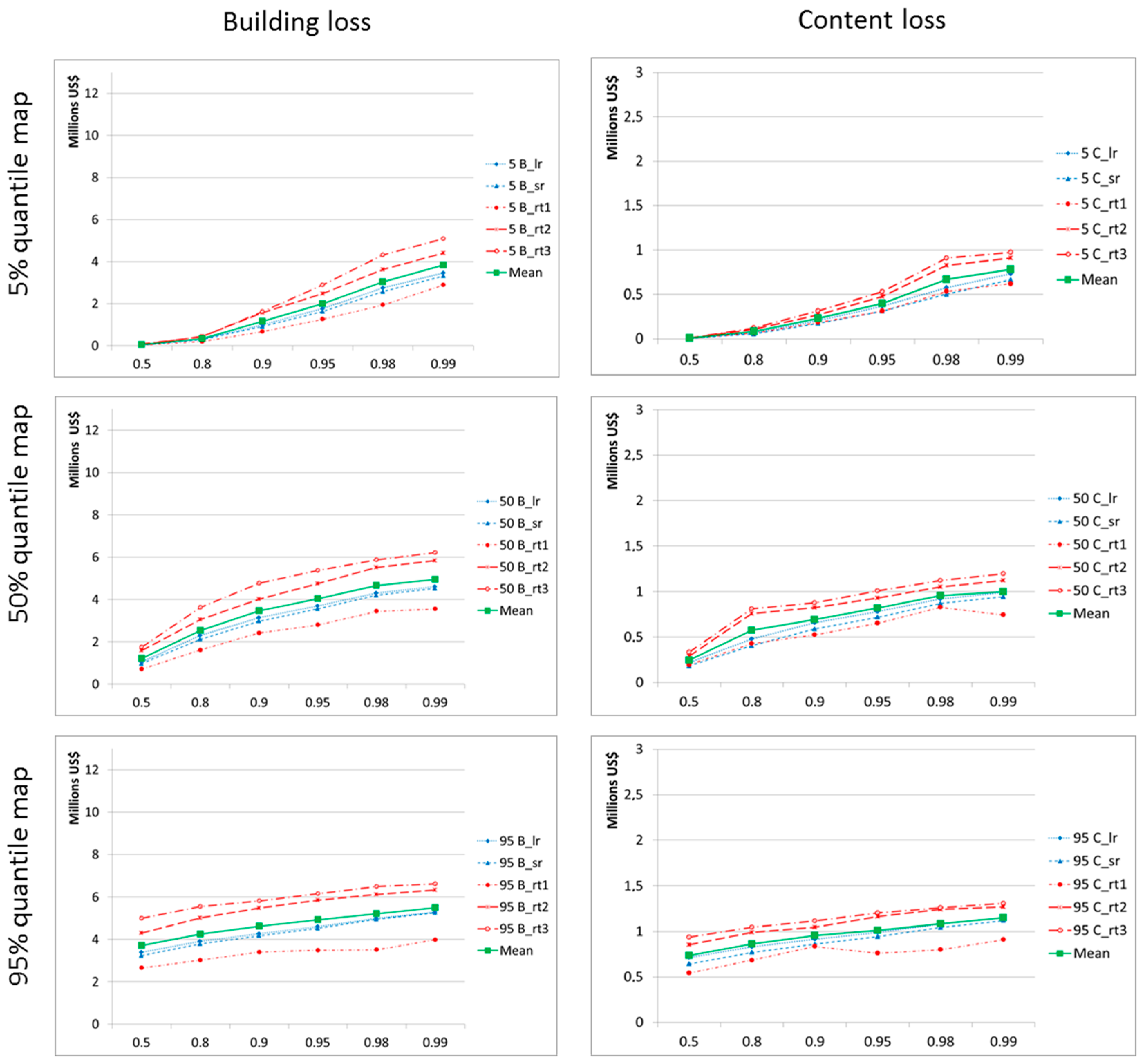
Figure 15.
Risk curves for different combined pluvial–fluvial flood scenarios and building and content losses. The blue lines indicate the linear and square root depth–damage functions. The red lines indicate the tree-base models with different numbers of predictors. The green line indicates the mean value of all models.


Table 1.
Input data for flood loss model development (source: [24]).
Table 1.
Input data for flood loss model development (source: [24]).
| Groups | Order | Abbreviation | Predictors | Range in Data Set |
|---|---|---|---|---|
| Hydrologic, hydraulic aspects | 1 | wst | Water depth | 2 cm to 120 cm above ground |
| 2 | d | Inundation duration | 4 to 1040 h | |
| Building/content characteristic | 3 | fsb | Floor space of building | 6 to 650 m2 |
| 4_1 | bv | Building value 1 | US$342 to 142,613 | |
| 4_2 | cv | Content value 1 | US$95 to 42,290 | |
| Abbreviation | Response Variables | Range in Data Set | ||
| Losses | A | Lossb | Building loss 1 | US$0 to 13,311 |
| B | Lossc | Contents loss 1 | US$0 to 4754 | |
Note: 1 Building value, content value, building loss, and content loss were calculated as prices of the year 2011.
Table 2.
Uncertainty of risk curves due to uncertainty in hazard maps and flood loss modeling.
| Flood Hazard Maps | Annual Probability of Non-Exceedance | Mean Absolute Difference of Risk Estimation (%) | |||||
|---|---|---|---|---|---|---|---|
| Building | Content | ||||||
| UHM 1 | ULM 2 | UHM-LM 3 | UHM | ULM | UHM-LM | ||
| Fluvial hazard maps | 0.5 | 59 | 12 | 85 | 65 | 11 | 90 |
| 0.8 | 33 | 15 | 51 | 45 | 12 | 61 | |
| 0.9 | 39 | 12 | 59 | 39 | 11 | 59 | |
| 0.95 | 34 | 12 | 48 | 36 | 9 | 54 | |
| 0.98 | 28 | 11 | 45 | 30 | 11 | 48 | |
| 0.99 | 28 | 10 | 51 | 28 | 9 | 41 | |
| Average | 44 | 14 | 68 | 49 | 12 | 71 | |
| Pluvial hazard maps | 0.5 | 110 | 11 | 150 | 111 | 8 | 141 |
| 0.8 | 82 | 16 | 112 | 77 | 16 | 97 | |
| 0.9 | 56 | 18 | 84 | 58 | 13 | 74 | |
| 0.95 | 40 | 19 | 67 | 41 | 13 | 60 | |
| 0.98 | 25 | 19 | 53 | 23 | 13 | 40 | |
| 0.99 | 17 | 17 | 39 | 19 | 14 | 35 | |
| Average | 66 | 20 | 101 | 66 | 15 | 89 | |
| Combined fluvial–pluvial hazard maps | 0.5 | 70 | 13 | 97 | 66 | 13 | 86 |
| 0.8 | 40 | 15 | 62 | 38 | 10 | 60 | |
| 0.9 | 28 | 14 | 49 | 29 | 12 | 50 | |
| 0.95 | 23 | 14 | 39 | 26 | 8 | 40 | |
| 0.98 | 17 | 12 | 35 | 22 | 11 | 37 | |
| 0.99 | 20 | 11 | 33 | 21 | 11 | 35 | |
| Average | 40 | 16 | 63 | 41 | 13 | 62 | |
Notes: 1 UHM: Mean absolute difference of risk estimation due to uncertainty of flood hazard map; 2 ULM: Mean absolute difference of risk estimation due to uncertainty of loss modeling; 3 UHM-LM: Mean absolute difference of risk estimation due to uncertainty of flood hazard map and loss modeling.
Table 3.
Expected annual damages for fluvial flood hazard: estimated building loss, content loss and total loss in US$1000 for the 5%, median and 95% quantile hazard maps. MAD indicates the mean absolute difference of EAD estimation caused by hazard uncertainty or by loss modeling.
Table 3.
Expected annual damages for fluvial flood hazard: estimated building loss, content loss and total loss in US$1000 for the 5%, median and 95% quantile hazard maps. MAD indicates the mean absolute difference of EAD estimation caused by hazard uncertainty or by loss modeling.
| Models/Quantile Map | Building Loss (US$1000) | Content Loss (US$1000) | Total Loss (US$1000) | |||||||||
|---|---|---|---|---|---|---|---|---|---|---|---|---|
| 5% | 50% | 95% | MAD (%) | 5% | 50% | 95% | MAD (%) | 5% | 50% | 95% | MAD (%) | |
| LR | 774 | 1522 | 2006 | 40 | 172 | 338 | 449 | 41 | 946 | 1860 | 2455 | 41 |
| SRR | 749 | 1497 | 1985 | 41 | 162 | 326 | 438 | 42 | 911 | 1823 | 2423 | 41 |
| RT1 | 556 | 1167 | 1564 | 43 | 134 | 264 | 370 | 45 | 689 | 1431 | 1935 | 44 |
| RT2 | 916 | 1736 | 2228 | 38 | 215 | 404 | 532 | 39 | 1131 | 2140 | 2760 | 38 |
| RT3 | 959 | 1859 | 2341 | 37 | 209 | 403 | 547 | 42 | 1168 | 2262 | 2889 | 38 |
| Average | 791 | 1556 | 2025 | 40 | 178 | 347 | 467 | 42 | 969 | 1903 | 2492 | 40 |
| MAD (%) | 26 | 23 | 19 | 59 * | 24 | 21 | 20 | 61 * | 25 | 22 | 19 | 59 * |
Note: * mean absolute difference of EAD estimates due to uncertainty in hazard and loss modeling.
Table 4.
Expected annual damages for the pluvial flood: estimated building loss, content loss and total loss in US$1000 for the 5%, median and 95% quantile hazard maps. MAE indicates the mean absolute difference of EAD estimation caused by hazard uncertainty.
Table 4.
Expected annual damages for the pluvial flood: estimated building loss, content loss and total loss in US$1000 for the 5%, median and 95% quantile hazard maps. MAE indicates the mean absolute difference of EAD estimation caused by hazard uncertainty.
| Models/Quantile Map | Building Loss (US$1000) | Content Loss (US$1000) | Total Loss (US$1000) | |||||||||
|---|---|---|---|---|---|---|---|---|---|---|---|---|
| 5% | 50% | 95% | MAD (%) | 5% | 50% | 95% | MAD (%) | 5% | 50% | 95% | MAD (%) | |
| LR | 287 | 1112 | 1923 | 74 | 60 | 233 | 409 | 75 | 347 | 1345 | 2332 | 74 |
| SRR | 265 | 1041 | 1862 | 77 | 51 | 203 | 379 | 81 | 316 | 1244 | 2241 | 77 |
| RT1 | 200 | 809 | 1487 | 80 | 54 | 200 | 332 | 69 | 254 | 1010 | 1819 | 78 |
| RT2 | 409 | 1481 | 2447 | 69 | 83 | 320 | 83 | 62 | 492 | 1801 | 2930 | 68 |
| RT3 | 447 | 1706 | 2707 | 66 | 93 | 347 | 513 | 61 | 540 | 2053 | 3220 | 65 |
| Average | 322 | 1230 | 2085 | 72 | 68 | 261 | 423 | 68 | 390 | 1490 | 2508 | 71 |
| MAD (%) | 43 | 40 | 32 | 113 * | 35 | 32 | 57 | 114 * | 41 | 39 | 30 | 110 * |
Note: * mean absolute difference of EAD estimates due to uncertainty in hazard and loss modeling.
Table 5.
Expected annual damages for the combined fluvial–pluvial flood: estimated building loss, content loss and total loss in US$1000 for the 5%, median and 95% quantile hazard maps. MAD indicates the mean absolute difference of EAD estimation caused by hazard uncertainty.
Table 5.
Expected annual damages for the combined fluvial–pluvial flood: estimated building loss, content loss and total loss in US$1000 for the 5%, median and 95% quantile hazard maps. MAD indicates the mean absolute difference of EAD estimation caused by hazard uncertainty.
| Models/Quantile Map | Building Loss (US$1000) | Content Loss (US$1000) | Total Loss (US$1000) | |||||||||
|---|---|---|---|---|---|---|---|---|---|---|---|---|
| 5% | 50% | 95% | MAD (%) | 5% | 50% | 95% | MAD (%) | 5% | 50% | 95% | MAD (%) | |
| LR | 1078 | 2596 | 3823 | 53 | 235 | 563 | 835 | 53 | 1314 | 3159 | 4659 | 53 |
| SRR | 1031 | 2504 | 3747 | 54 | 217 | 523 | 796 | 55 | 1248 | 3027 | 4543 | 54 |
| RT1 | 768 | 1949 | 2977 | 57 | 189 | 460 | 683 | 54 | 957 | 2409 | 3660 | 56 |
| RT2 | 1339 | 3169 | 4550 | 51 | 304 | 707 | 982 | 48 | 1643 | 3876 | 5532 | 50 |
| RT3 | 1429 | 3497 | 4898 | 50 | 306 | 733 | 1028 | 49 | 1735 | 4230 | 5926 | 50 |
| Average | 1129 | 2743 | 3999 | 52 | 250 | 597 | 865 | 51 | 1379 | 3340 | 4864 | 52 |
| MAD (%) | 31 | 30 | 25 | 80 * | 25 | 24 | 21 | 75 * | 30 | 29 | 24 | 79 * |
Note: * mean absolute difference of EAD estimates due to uncertainty in hazard and loss modeling.
© 2017 by the authors. Licensee MDPI, Basel, Switzerland. This article is an open access article distributed under the terms and conditions of the Creative Commons Attribution (CC BY) license (http://creativecommons.org/licenses/by/4.0/).
Share and Cite
MDPI and ACS Style
Chinh, D.T.; Dung, N.V.; Gain, A.K.; Kreibich, H. Flood Loss Models and Risk Analysis for Private Households in Can Tho City, Vietnam. Water 2017, 9, 313. https://doi.org/10.3390/w9050313
AMA Style
Chinh DT, Dung NV, Gain AK, Kreibich H. Flood Loss Models and Risk Analysis for Private Households in Can Tho City, Vietnam. Water. 2017; 9(5):313. https://doi.org/10.3390/w9050313
Chicago/Turabian StyleChinh, Do Thi, Nguyen Viet Dung, Animesh K. Gain, and Heidi Kreibich. 2017. "Flood Loss Models and Risk Analysis for Private Households in Can Tho City, Vietnam" Water 9, no. 5: 313. https://doi.org/10.3390/w9050313
Note that from the first issue of 2016, this journal uses article numbers instead of page numbers. See further details here.