
Estimation of Residence Time and Transport Trajectory in Tieshangang Bay, China


1
School of Hydraulic Engineering, Changsha University of Science & Technology, Changsha 410114, China
2
Hunan Province Key Laboratory of Water, Sediment Sciences & Flood Hazard Prevention, Changsha 410114, China
3
International Research Center of Water Science & Environmental Engineering, Changsha University of Science & Technology, Changsha 410114, China
4
Department of Geography, University of Wisconsin-Milwaukee, Milwaukee, WI 53211, USA
*
Author to whom correspondence should be addressed.
Water 2017, 9(5), 321; https://doi.org/10.3390/w9050321
Submission received: 11 January 2017
/
Revised: 25 April 2017
/
Accepted: 26 April 2017
/
Published: 2 May 2017
Abstract
:The pollutant residence time and transport trajectory in Tieshangang Bay are considered to have significant effects on deteriorating water quality. To understand the pollutant transport behaviors in Tieshangang Bay, we developed a combination model (MIKE 21 FM) of the hydrodynamic module and particle tracking module. Simulation results suggest that the water velocities in the west and east troughs (near the entrance of the bay) are distinctly higher than any other areas. Meanwhile, small semi-enclosed bays adjacent to the shoreline could affect local water flow patterns, thereby causing gyres within them. The residence time of pollutants in Tieshangang Bay is significantly affected by seasonal variations (i.e., the residence time of pollutants in Tieshangang Bay in winter is less than that in summer). The results of transport trajectory simulations reveal that the bay head is a slow flushing zone, while the entrance of the bay (west trough) can be identified as a fast flushing zone.
1. Introduction
Bays are an important part of the coastal ocean. In recent years, the development of many bays (e.g., Tieshangang Bay, located in Southern China) and their coastal areas has been intensified and expanded, due to their unique hydrogeological environment, convenient sea transportation conditions, and rich marine resources. However, increasingly frequent human activities have caused serious disturbance and pressure in and on bays and coastal areas [1], resulting in eutrophication of water bodies, declining biodiversity, the frequent occurrence of toxic and harmful red tides, etc. Although the coastal marine water body has a certain self-purification capacity, it only accounts for about 5‰ of the world’s marine water bodies, while it has to accommodate 80% of the global organic mass and 75–90% of suspended river sediment, as well as pollutants [2]. Moreover, most of the bays have semi-enclosed geomorphic features. The depth and width of the waters are gradually reduced in the inland direction. The self-purification capacity of the water body is related to its topographic features, tides, waves, and currents, etc.
Meanwhile, the exchange of the water body in bays is an important hydrodynamic process in the ocean circulation. Pollutants in the bay are mixed with surrounding water bodies via physical processes such as convective transport and dilution diffusion [2]. In the process of exchange with external water, pollutant concentration in the bay gradually decreases, resulting in improved water quality. The progress and extent of the whole convection-diffusion, as well as the mixing-exchange process, are closely related to the self-purification capacity, environmental capacity, nutrient transport, and ecological environment, etc. Therefore, water exchange has been increasingly investigated in estuarine and coastal water quality studies in recent years [3,4,5,6,7]. As a concept related to water exchange, transport time scales such as water age, flushing time, residence time, and transient time are often used as parameters for representing the time scale of the physical transport processes [5,8,9,10,11,12]. These time scales can describe how some water quality parameters (e.g., eutrophication, red tides, and chlorophyll-a concentration, etc.) change with different conditions [12]. Water exchange in a bay is the result of the complex interplay of the abovementioned factors (e.g., geographic features, waves, tides, winds, and currents), and therefore, knowledge of the transport time scale has great significance in protecting the marine environment and maintaining the ecological balance of the coastal seas.
Tieshangang Bay is a part of the Beibu Gulf, located in the Southern China. In recent years, with the development and utilization of the marine resources in the Beibu Gulf, water pollution in the Beibu Gulf is becoming more and more serious. According to the industrial pollution discharge data from the Guangxi Statistical Yearbook in 2009, the total discharge of pollutants increased by 1–1.5 times than that of 2003 [13]. It was reported that a number of abnormal seawater quality accidents occurred from January to September 2013. The monitoring results showed that the main reasons for the obvious deterioration of seawater quality were due to the high level of inorganic nitrogen, active acid salt, and chemical oxygen demand. Moreover, these areas are mainly distributed in estuaries and the sewage areas of cities. Additionally, a number of marine activities, such as ship traffic, accident pollution, and oil spills, also bring pollution to the ocean. The water exchange rate is slow in Tieshangang Bay because of the synthetic effect of the semi-enclosed topography constraints, weak local sea currents, and diurnal tides [2,14,15]. Therefore, it is difficult for pollutants to spread out of the bay. The long-term accumulation has resulted in local environmental pollution in Tieshangang Bay. The present situation shows that seawater eutrophication becomes more and more serious—especially in estuary and harbor areas. Hence, it is very important to know the exchange characteristics between the bay water body and the external water body. However, previous studies have mainly focused on the effect of water self-purification capacity on the ecological environment from the changes of the biological distribution aspect [16]. A few researchers have tried to simulate the water exchange characteristics by using particle-tracking techniques [14] or dye-tracer techniques [15]. However, no references or estimates that consider the effect of seasonal behavior on water exchange in Tieshangang Bay are available in the literature. Therefore, the investigation of the seasonal transport time scale in Tieshangang Bay adds to the novelty of the current study.
In this context, detailed transport time scales of Tieshangang Bay were explored using the hydrodynamic module of MIKE 21 FM (flow model) linked to a particle tracking module with a long-time simulation (2004–2015). The main objectives were to: (1) investigate the influence of the bay’s hydrodynamics on the pollutant transport pathways within the bay; (2) explore the effect of seasonal behaviors on the residence time in Tieshangang Bay; and (3) examine the transport trajectory of each sub-region, which can facilitate identification of the fast and slow flushing zones, as well as exploration of the accident pollution transport pathways. The current study represents a first attempt to investigate the comprehensive pollutant transport behavior in Tieshangang Bay with seasonal variations by a combination model (MIKE 21 FM) of the hydrodynamic module and particle tracking module with a long time simulation (2004–2015). This study provides useful information for maintaining the ecological balance of Tieshangang Bay and similar semi-enclosed bays.
2. Materials and Methods
2.1. Study Area
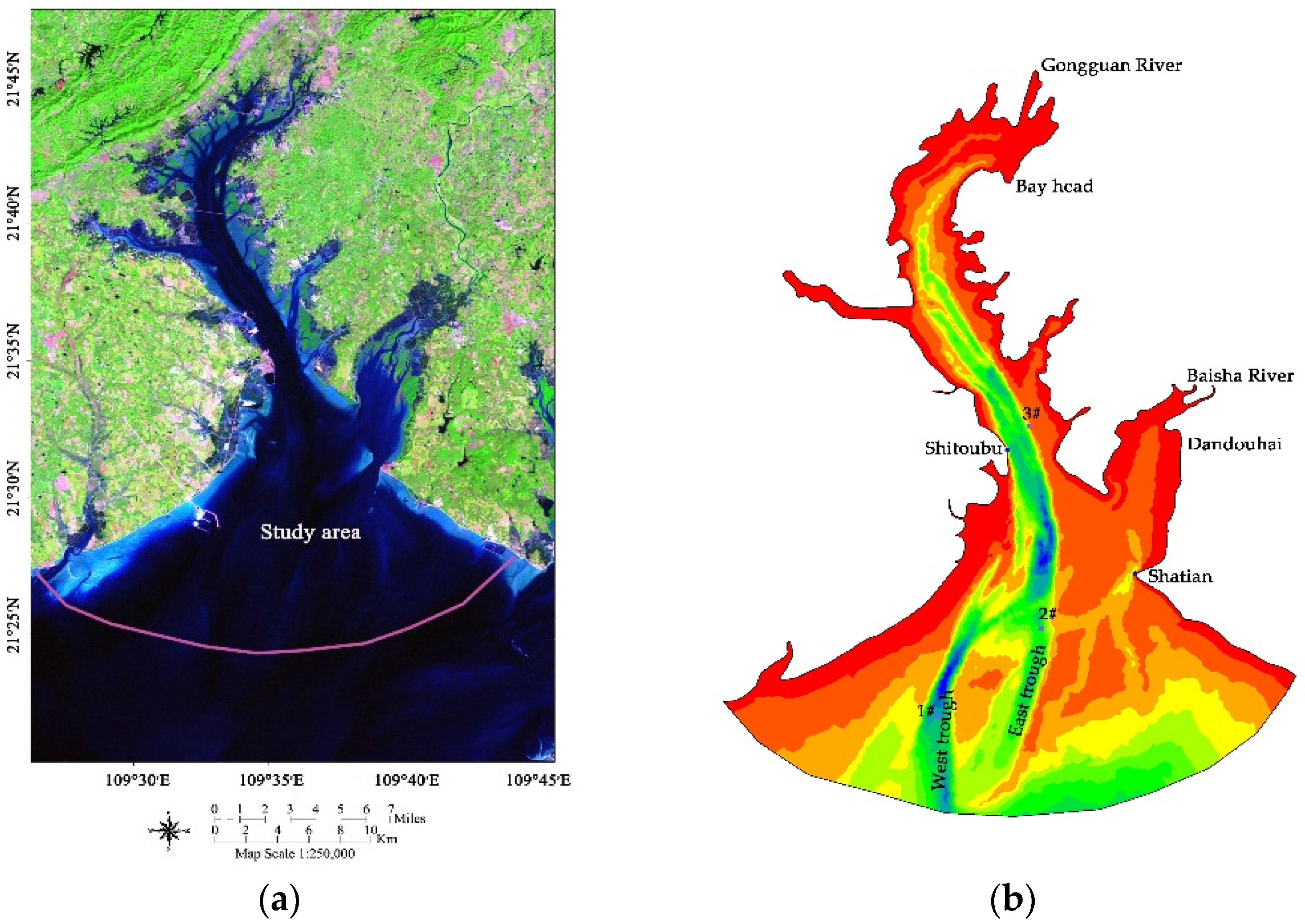
Tieshangang Bay is located at the northeast of Beibu Gulf of China, which lies between 21°28′–21°45′ N, 109°26′–109°45′ E. The mouth of the bay is about 32 km wide; the coastline of the entire bay is approximately 170 km; and the area is nearly 340 km2 [17]. The topography of the bay is high in the north and low in the south. It is inclined from land to sea, with a gentle slope (0.5‰–2.0‰) and a depth of 0–20 m. The submarine slope and intertidal shoal with a shallow water depth less than 2.5 m are 280 km2, accounting for 82% of the total area [18]. The tidal regime is irregularly diurnal, with the mean and maximum tidal ranges of 2.89 m and 6.25 m, respectively [17,19]. The water exchange is mainly affected by the tide because no large river flows to the bay [17]; i.e., the inflow discharge of Baisha River and Gongguan River is only 2 m3/s and 16 m3/s, respectively [14]. Hence, we did not consider the influence of the river on the residence time in the bay during the simulation.
2.2. Method
In this study, the hydrodynamic module—in conjunction with the particle tracking module of Mike 21 FM, which is a 2D depth-averaged model—was employed to investigate the transport behaviors in Tieshangang Bay. We used the hydrodynamic module to obtain flow features of Tieshangang Bay. The particle tracking module was applied to track the spatial distributions of water particles, and thus to provide the transport trajectory using the Lagrangian random-walk technique [20,21]. It can also examine the water residence and travel time of Tieshangang Bay. The MIKE 21 model has already been successfully applied in exploring different water bodies, such as Poyang Lake (China) [21], Vistula Lagoon (Poland and Russia) [22], the Gulf of Kachchh (India) [23], Alberni Inlet (Canada) [24], and Chilika Lagoon (India) [25]. Hence, we only give a brief description of the model here.
2.2.1. Hydrodynamic Module
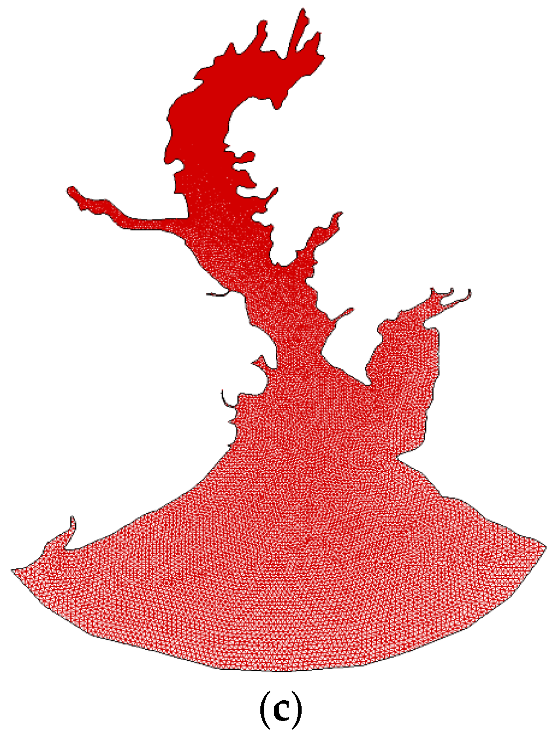
The bathymetry of the bay was based on surveyed data updated in 2008 (Figure 1b). We constructed the seabed using triangular unstructured grids based on the measured topographic information. The mesh resolution of the open boundary of the open sea is 300 m, and a higher mesh resolution (20 m) was applied to bay head (Figure 1c). Therefore, a total of 25,442 nodes and 48,926 triangular elements were included in the grid. The minimum and maximum element sizes were 20 and 300 m, respectively. The Manning’s roughness of Tieshangang Bay was set to 32 m1/3/s [14,15,26]. The tidal boundary condition was provided by the tidal prediction based on the Global Tide Model data in the Mike 21 Toolbox [27], and the inflow discharge of the rivers were not considered in this model, as discussed in Section 2.1.
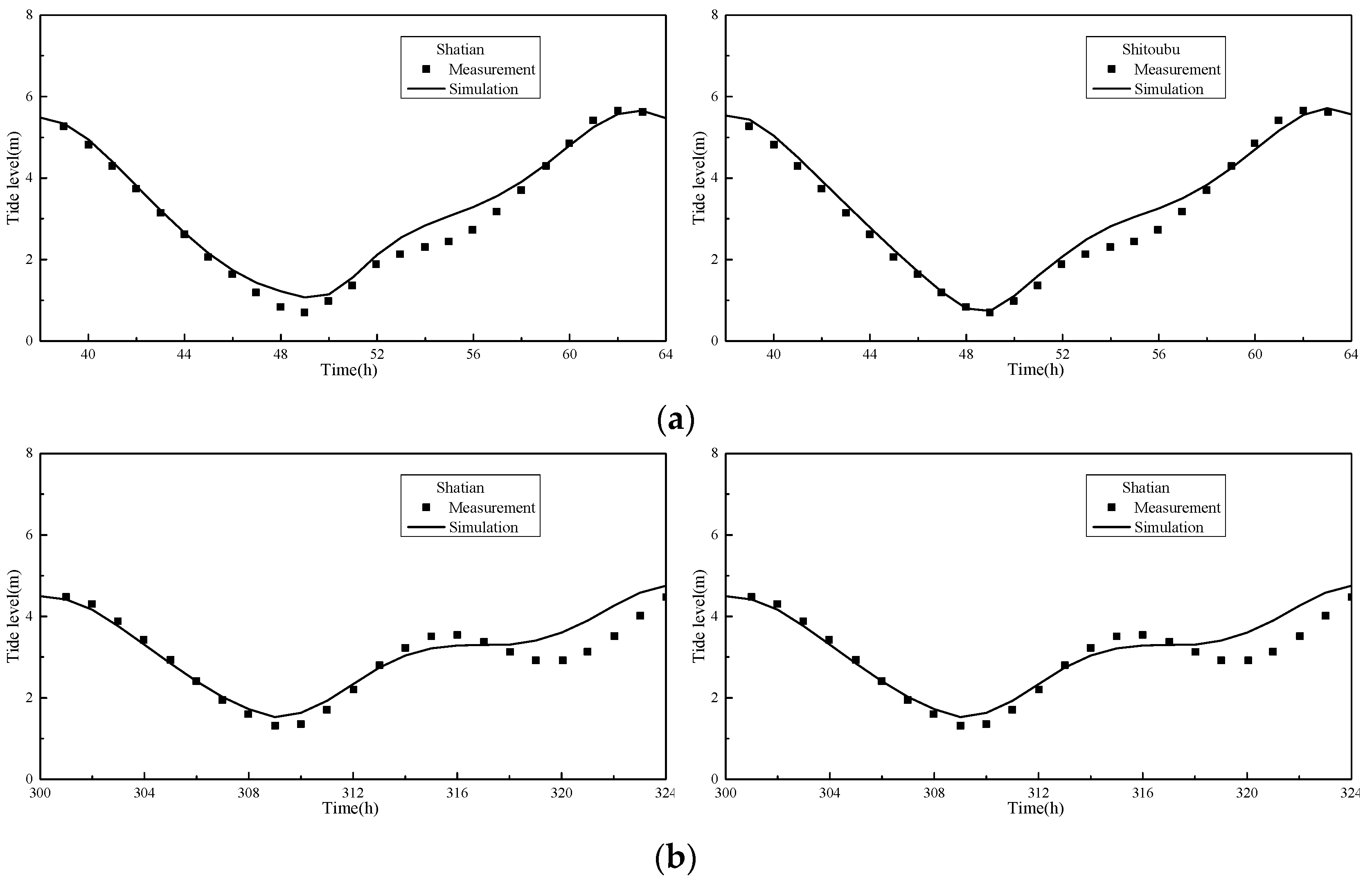
The performance of MIKE 21 FM was validated against (1) the tide level records at Shatian and Shitoubu, which is obtained from the local tide gauge stations; and (2) the magnitude and direction of velocity records at three temporary measurement points in Tieshangang Bay (Figure 1b). The velocities were obtained from the previous study on this area [15], which were measured in 1-m cell size and 1 Hz data rate with a sampling time of 30 min using Aquadopp Profiler (Nortek Co., Ltd., Bærum, Norway). The results show that the model appears to be in agreement with the tidal level and direction for spring and neap tides (Figure 2, Figure 3 and Figure 4). However, the magnitude of the velocities might be under- or over-estimated in this model (Figure 2 and Figure 3), partly because of the complex bathymetry and meteorological condition.
2.2.2. Particle Tracking Module
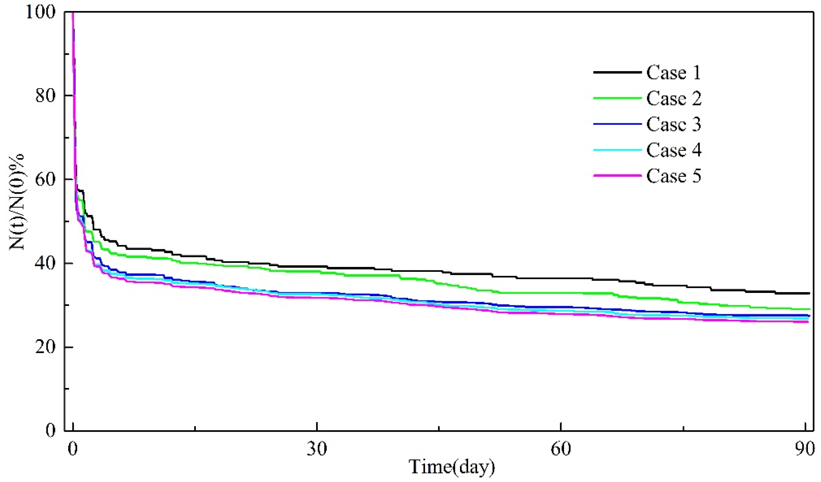
The Lagrangian particle-tracking technique has been widely used to estimate the transport time scale in a variety of water bodies [25,28,29]. In this study, the particle-tracing module—as driven by the hydrodynamic module of MIKE 21 FM—was applied to estimate the water residence time and the sub-zone transport trajectory of Tieshangang Bay. The mean residence time of the bay is estimated by the e-folding time [30], which is the time when the average of the conservative particles in the bay is decreased to 1/e (i.e., 33%, e-folding) of the initial particle numbers [31]. In an ideal model, one would assign one particle to each grid cell in the particle tracking module. However, it is impossible to apply this to the current study because of the large horizontal scale of Tieshangang Bay. Hence, a particle number sensitivity analysis was carried out first, considering five different numbers of particles (see in Table 1).
Figure 5 shows the sensitivity analysis results. There is a significant discrepancy in the calculation of the percentage of particles remaining in the bay. Case 1 and Case 2 exhibit an overestimation of the residence time due to the insufficiently-released particles. In the view of Case 3, there is a small discrepancy for the first 10-day simulation compared to Case 4 and Case 5. However, no relevant differences are observed between the percentages of particles remaining in the bay calculated using 1830 particles and 4430 particles. A maximum error smaller than 5% was found between the results obtained from Case 4 and Case 5. Based on previous results, 1830 particles with a resolution of 500 m × 500 m were selected for the present study.
We performed separate simulations for the water residence time of Tieshangang Bay because it is located in the East Asian monsoon region, which shows notable seasonal dynamics (i.e., southwest winds in summer and northeast winds in winter) [2]. The releases were assumed to take place in summer and winter with the meteorological data obtained from QUICKSCAT [32], respectively. The particle tracking module of Mike 21 FM was also used to calculate the transport trajectory in Tieshangang Bay. Three sub-zones (i.e., the bay head; Shitoubu, middle of the bay; and the west trough, the entrance of the bay; Figure 1b) were chosen to distinguish the fast and slow flushing zones of the bay.
3. Results
3.1. Residence Time for Tieshangang Bay
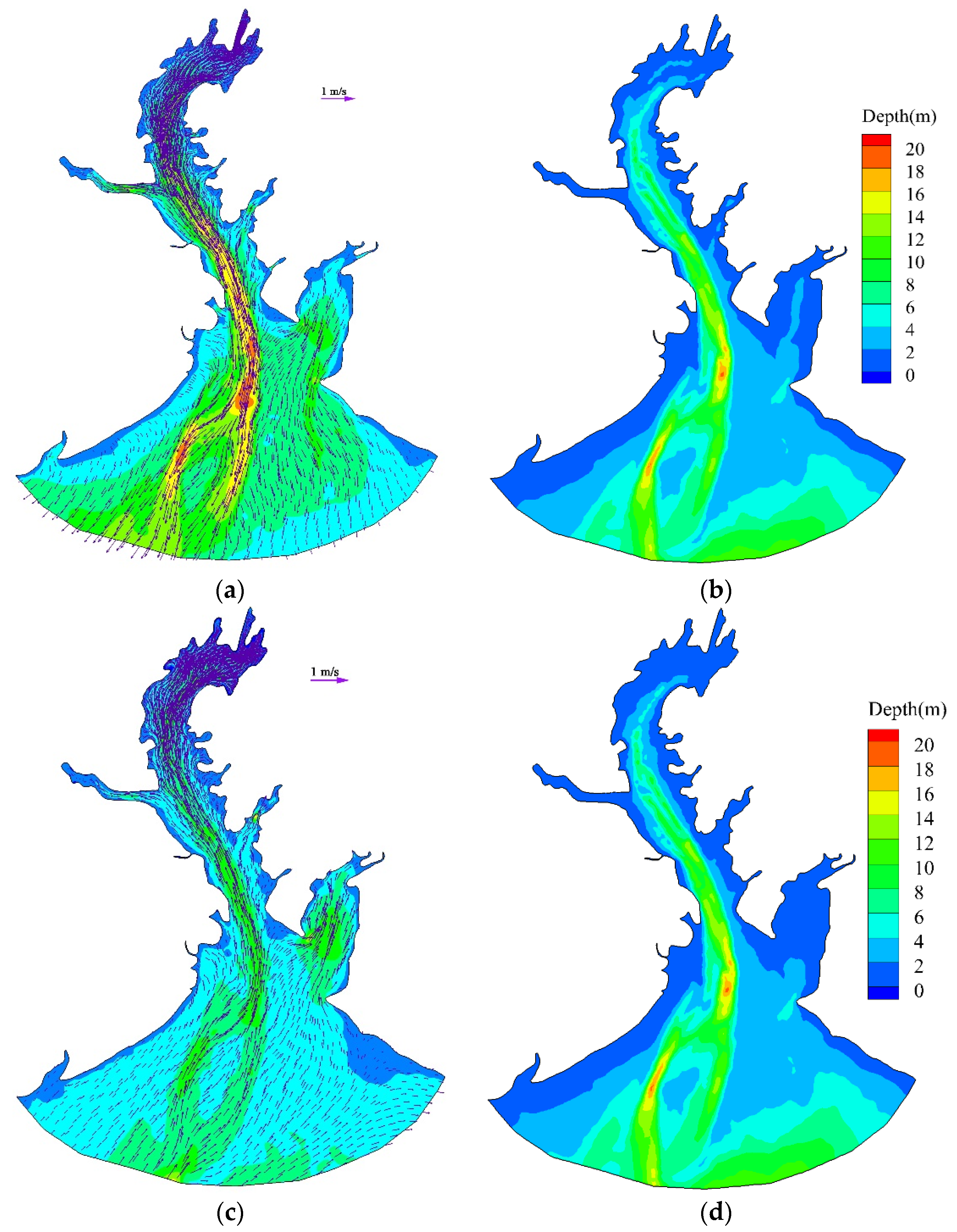
Flow field characteristics have significant influences on the distribution and transport of pollutants within Tieshangang Bay. Hence, the general flow behaviors in the bay which are generated by the hydrodynamic module should be analyzed first. Figure 6 shows the spatial distribution of the water velocity and depth of flood and ebb currents in Tieshangang Bay (e.g., 1 June 2008). A distinct difference in the magnitude of 0.3–0.4 m/s was observed between the bay’s main flow channels (i.e., the water depth ranged from 8 to 20 m; Figure 6b,d) and the shallow water areas (i.e., shallow water depth roughly <8 m; Figure 6b,d). The water velocities in the west and east troughs (Figure 1b) near the entrance of the bay (up to 0.7 m/s and 0.4 m/s for flood and ebb currents, respectively) were distinctly higher than any other areas (about 0.3 m/s and 0.1 m/s for ebb and flood currents, respectively) of Tieshangang Bay (Figure 6a,c), suggesting the strong effect of the tide on these places. The difference is partly because of the complex topography of the bay. The tide flows into or out of the bay with considerably narrower cross-sections in the main channel, which may increase the water velocity here (Figure 6b). In general, the velocity of the ebb current is larger than that of the flood current (Figure 6a,c).
Figure 7 shows that the streamline of the flood and ebb currents of spring (e.g., 4 June 2008) and neap tides (e.g., 10 June 2008) respectively, during June. In general, the large-scale tidal flow patterns generated by the hydrodynamic module show distinct south–northward and north–southward flows for flood and ebb currents, respectively, in the entire bay (see the streamlines in Figure 7). During the flood period, the tidal currents flow into the bay along the west and east troughs, and the mainstream of the tidal currents is consistent with the direction of the channel. The direction of the tidal currents in the bay head switches from northwest to northeast because of the constraint of the topography. The general trend of the ebb-flow distribution is opposite to that of the flood current. The tidal currents in the bay head flow southward, and the water in the bay flows out along the channel in the south and southwest directions. Additionally, the local water flow patterns in the bay could be influenced by the small semi-enclosed bays adjacent to the shoreline, generally causing gyres in them (i.e., the streamlines are closed; Figure 7a,b,f). The tidal flow patterns indicate that the inflows from the outside sea (or outflow from the bay) pass through the shallow water areas and further flow into the bay’s main flow channels. Therefore, the tidal flow velocities along the bay’s main channels are obviously higher than those of the water velocities in the shallow water areas (Figure 7).
The particle tracking module was applied to simulate the residence time in Tieshangang Bay under two kinds of hydrodynamic conditions; i.e., tidal currents with summer monsoon (south wind, 1 May–31 July, 2004–2015) and tidal currents with winter monsoon (northeast wind, 1 November–31 January, 2004–2015). Tieshangang Bay was evenly distributed with 1830 virtual particles, and the distribution of water particles in the 92 days was simulated in each season. The time step size was calculated as 1800 s. Figure 8 and Figure 9 illustrate the simulation results of the residence time for Tieshangang Bay in summer and winter seasons, respectively. The initial percentage of conservative particles was set to 100% (i.e., ε = N (t)/N (0) = 1) [21], and the percentage of the particles remaining in the bay (i.e., ε = N (t)/N (0)) was recorded, as shown in Figure 8 and Figure 9.
Figure 8 illustrates the results of residence time for the bay in summer for 12-year simulations (2004–2015). The water residence time has a large change between years. For example, the mean residence time (i.e., 33% of the initial particles remaining in the bay) arranges from 14.8 days to over 92 days among the simulation years. However, the decreasing trend of the particles is similar for the 12-year simulations, which can be divided into fast and slow decrease phases. Take 2008 as an example: the particles decrease sharply to 50% of the initial particles in the first 10 days (i.e., fast decrease phase). After that, the slope of the time-dependent particle curve becomes flat (i.e., slow decrease phase).
Figure 9 illustrates the results of residence time for the bay in winter for 12-year simulations (2004–2015). The water residence time is also different between years; e.g., the mean residence time varies from 5.9 days to 90 days, except for 2013 (over 92 days). The decreasing trend can also be divided into fast and slow decrease phases. Taking 2008 as an example, the reduction rate of particles was, however, faster than that in summer. It only takes 1.3 days to reduce the particles by 50% in the bay, which is about 8.7 days less than that in summer. The rapid reduction phase continued for about 8.5 days, and only 34.1% of the initial particles remained in the bay. After that, it only decreased by 7.5% of the initial particles in the next 83.3-day simulation.
The residence time when 50% of the initial particles remained in the bay in summer and winter is shown in Figure 10. Comparing simulations of summer and winter, one can note that the residence time (50% particles remaining in the bay) has a large change (5.9 days to 90 days) in summer, while it shows a relatively shorter time scale (less than 10 days for all simulated years) in winter. Table 3 shows the mean residence time in summer and winter from 2004 to 2015, respectively. In summer, there were five years (i.e., 2006, 2009, and 2012–2014) where the mean residence time was over 92 days. The mean residence time of the other seven years ranged between 14.9 days for 2004 and 70 days for 2010. In winter, however, only one year’s (i.e., 2013) mean residence time was over 92 days. The mean residence time of the other eleven years ranged from 8.6 to 90 days. Based on the above analysis, the residence time in winter is less than that in summer, indicating that the water exchange in winter is more active than that in summer.
3.2. Transport Trajectories for Different Released Sources
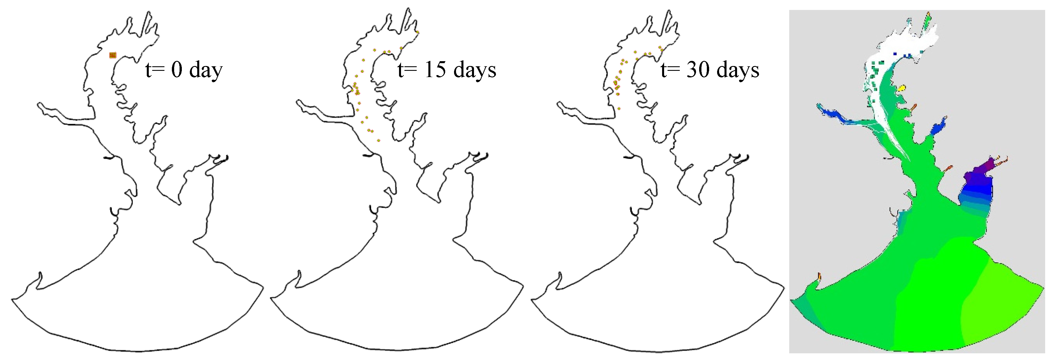
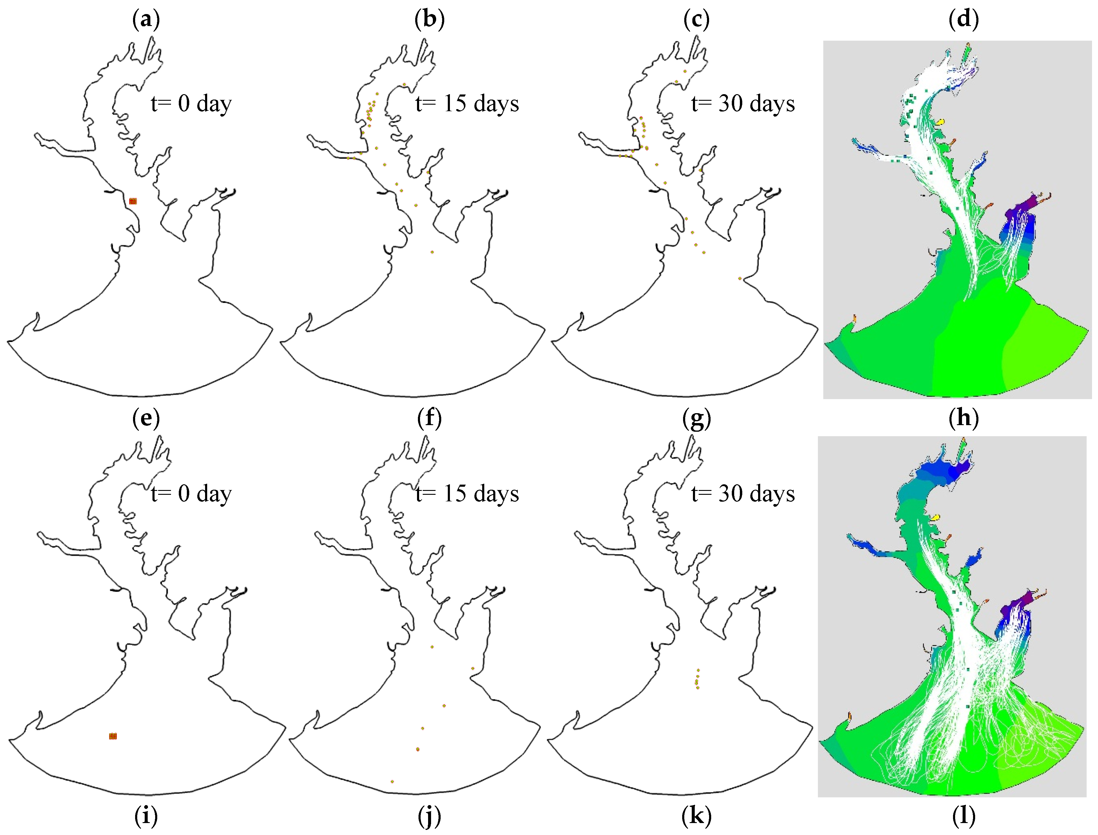
In order to identify the fast and slow flushing zones in the bay, the tracer particle release source was used to simulate the water transport in three selected sub-zones (i.e., the bay head; Shitoubu, middle of the bay; and the west trough, the entrance of the bay; Figure 11a,e,i) in Tieshangang Bay. A one-month simulation (i.e., from 1 June to 1 July 2008) was conducted, and the particle positions were recorded in each hour. Figure 11 shows the spatial distribution of particles released from each selected sub-zone after 0, 15, and 30 days in the bay.
The particles released in the bay head area were driven to the northeast of the bay by the flood current and to southwest of the bay by the ebb current. However, the particles did not move out of the bay (Figure 11d) because of the short time of the ebb current. Therefore, all of the released particles remained in the bay head during the simulation, which is likely to cause the accumulation of pollutants. Particles released in the Shitoubu area—located in the middle of Tieshangang Bay—moved back and forth with the tide currents along the main channel in the middle of the bay. Due to the dispersion of shallow water, a part of the particles moved into the small bay (e.g., Dandouhai) under the force of the tidal current during the simulation. The transport pathways cover almost the entire inner bay after 30 days simulation (Figure 11h). The particles released in the west trough of the channel near the shelf—located in the center of the entrance to Tieshangang Bay—move with the prevailing flow of Tieshangang Bay. After 15 days, 70% of the initial particles were flushed out of the bay (Figure 11j), and almost 80% of the released particles moved to the outside sea after 30 days simulation (Figure 11k). Most of the flushed particles finished their trajectory near the south and southeast bay (Figure 11l), which coincides with the tidal current patterns (from west to east) during the high water slack (Figure 7b) or the low water slack (Figure 7g). The transport pathways covered almost the entire Tieshangang Bay, except for the bay head.
4. Discussion
To understand the mechanism of the transport behavior in a semi-enclosed bay, we developed a combination model of the hydrodynamic module and particle tracking module to simulate the residence time and transport trajectory in Tieshangang Bay with seasonal variations. The current work represents a first attempt to use a combination model to offer comprehensive insights into the transport behaviors with seasonal variability of Tieshangang Bay relative to previous studies [14,15,16].
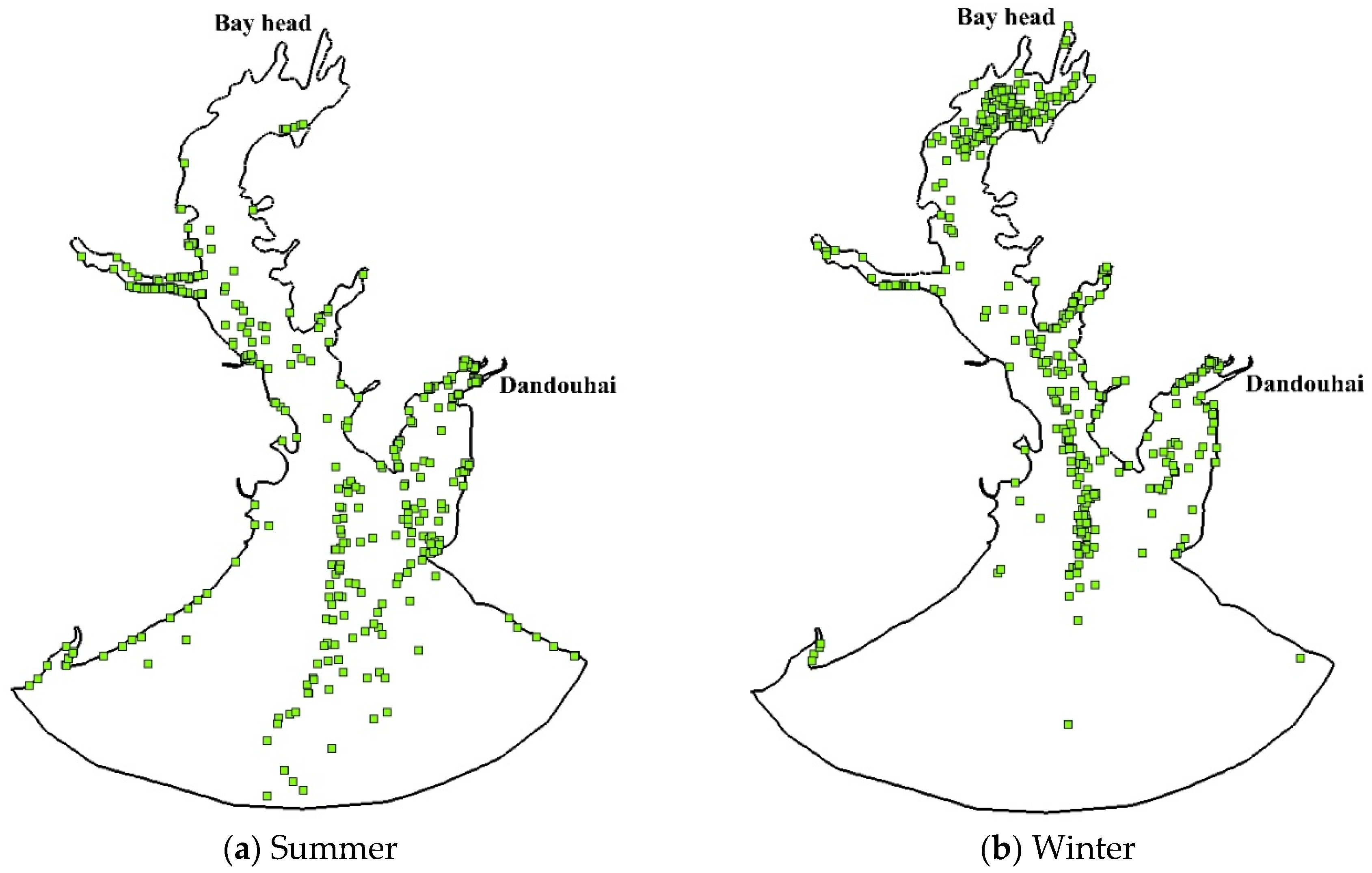
The particle distributions in the bay after 92-day simulations of summer and winter are shown in Figure 12 (taking 2008 as an example). In summer, the particles are more likely to accumulate in small semi-enclosed bays (e.g., Dandouhai, Figure 12a). This can be explained by the fact that the velocities of the ebb current are larger than that of the flood current (Figure 7a,c), leading to the particles moving southward. Moreover, the gyres are more likely generated in small bays (Figure 7a,f), leading to the southward particles gathering there. In winter, a large number of the remaining particles stay in the bay head and the small bays (Figure 12b). This is partly because the particles are forced to move to the bay head during the flood current, and there is not enough time to bring particles out of the bay head with the ebb current. The gyres also promote the particles accumulating in small bays. The results of winter water transport show different characteristics compared to the summer based on the above analysis.
The transport trajectories simulation shows that the particles released from the bay head remain in the bay head, indicating that this area is a slow flushing zone, which inhibits the diffusion of pollutants. Although the particles released from Shitoubu also remain in the bay after a 30-day simulation, the transport pathway covers the entire inner bay, which is beneficial for pollutants diffusion in this area (Figure 11h). When the particles are released from the west trough, the tidal currents are favorable to push the particles travelling away from the released area and towards the north side of the bay with the flood current, and then move to the south side of the bay with the ebb currents. Finally, some particles are flushed out of the bay during the high or low water slack because of the west–east current patterns (Figure 7b,g). Therefore, the entrance area of the bay can be identified as the fast flushing zone in which pollutants would quickly travel to the outside sea.
This study developed a very practical combined model approach to estimate the residence time of Tieshangang Bay. With some caution, it could also be applied to solve the same problem for similar tide-dominant semi-enclosed bays.
- (1)
- Some factors (e.g., degradation values, vertical dispersion, and settling velocity, etc.) that affect pollutant transport behavior were not incorporated in the current model, since it is the first time that a combined model has been employed to quantify the mean residence time of Tieshangang Bay based on long-time simulation (2004–2015). Hence, future study may be necessary to consider the abovementioned factors for more accurate estimation of the pollutant transport behavior.
- (2)
- The assumption of the 2D depth-averaged flow has the ability to represent the flow field of Tieshangang Bay in the current study. However, the water depth of the bay may reach up to 20 m in the main stream of the bay. Hence, it is reasonable to expect the pollutant transport behavior may change with different water depths. Therefore, the current study could be extended to a 3D model approach to investigate the water exchange of a similar bay.
5. Conclusions
In order to understand the pollutant transport behaviors in Tieshangang Bay, we integrated a hydrodynamic module (using MIKE 21 FM) and a particle tracking module to simulate the physical processes of pollutants. The mean residence time of pollutants in Tieshangang Bay was estimated in summer and winter, respectively. The fast and slow flushing zones of Tieshangang Bay were also identified by tracking the transport trajectory of particles released in selected sub-zones. The following conclusions can be drawn from the study:
The hydrodynamic module simulation results suggest that the water velocities in the west and east troughs (near the entrance of the bay) are distinctly higher than any other areas, which is partly because of the topography of the bay. Meanwhile, small semi-enclosed bays adjacent to the shoreline could affect local water flow patterns, thereby causing gyres within them.
The particle tracking module results revealed that water exchange in Tieshangang Bay is significantly affected by seasonal behaviors. The mean residence time of pollutants in Tieshangang Bay in winter is less than that in summer. Hence, the water exchange in winter is better than that in summer. Based on the transport trajectories analysis, the bay head could be identified as the slow flushing zone, while the entrance area of the bay can be identified as the fast flushing zone.
Acknowledgments
This research was partially supported by the National Natural Science Foundation of China (51239001 and 51509023), Natural Science Foundation of Hunan Province, China (2016JJ3011), and the Scientific Research Fund of Hunan Provincial Education Department, China (16C0056). We received funds for covering the costs to publish in open access. QuikScat (or SeaWinds) data are produced by Remote Sensing Systems and sponsored by the NASA Ocean Vector Winds Science Team. Data are available at www.remss.com.
Author Contributions
Changbo Jiang and Yizhuang Liu analyzed the data and wrote the manuscript; Yuannan Long and Changshan Wu designed the modeling approach.
Conflicts of Interest
The authors declare no conflict of interest. The founding sponsors had no role in the design of the study; in the collection, analyses, or interpretation of data; in the writing of the manuscript, and in the decision to publish the results.
References
- Bilgili, A.; Proehl, J.A.; Lynch, D.R.; Smith, K.W.; Swift, M.R. Estuary/ocean exchange and tidal mixing in a gulf of Maine estuary: A lagrangian modeling study. Estuar. Coast. Shelf Sci. 2005, 65, 607–624. [Google Scholar] [CrossRef]
- Wang, L.N. Analysis of Hydrodynamic Characteristics Based on Random Walk Model in Tonkin Gulf. Master’s Thesis, Xiamen University, Xiamen, China, 2014. (In Chinese). [Google Scholar]
- Delhez, É.J.; Heemink, A.W.; Deleersnijder, É. Residence time in a semi-Enclosed domain from the solution of an adjoint problem. Estuar. Coast. Shelf Sci. 2004, 61, 691–702. [Google Scholar] [CrossRef]
- Fukumoto, T.; Kobayashi, N. Bottom stratification and water exchange in enclosed bay with narrow entrance. J. Coast. Res. 2005, 21, 135–145. [Google Scholar] [CrossRef]
- Yuan, D.; Lin, B.; Falconer, R.A. A modelling study of residence time in a macro-tidal estuary. Estuar. Coast. Shelf Sci. 2007, 71, 401–411. [Google Scholar] [CrossRef]
- Guo, W.; Wu, G.; Liang, B.; Xu, T.; Chen, X.; Yang, Z.; Jiang, M. The influence of surface wave on water exchange in the Bohai Sea. Cont. Shelf Res. 2016, 118, 128–142. [Google Scholar] [CrossRef]
- Nguyen, T.D.; Hawley, N.; Phanikumar, M.S. Ice cover, winter circulation, and exchange in Saginaw Bay and Lake Huron. Limnol. Oceanogr. 2017, 62, 376–393. [Google Scholar] [CrossRef]
- Zimmerman, J.T.F. Mixing and flushing of tidal embayments in the western Dutch Wadden Sea part I: Distribution of salinity and calculation of mixing time scales. Neth. J. Sea Res. 1976, 10, 149–191. [Google Scholar] [CrossRef]
- Dabrowski, T.; Hartnett, M.; Olbert, A.I. Determination of flushing characteristics of the Irish Sea: A spatial approach. Comput. Geosci. 2012, 45, 250–260. [Google Scholar] [CrossRef]
- Nguyen, T.D.; Thupaki, P.; Anderson, E.J.; Phanikumar, M.S. Summer circulation and exchange in the Saginaw Bay-Lake Huron system. J. Geophys. Res. Oceans 2014, 119, 2713–2734. [Google Scholar] [CrossRef]
- Li, Y.; Zhang, Q.; Yao, J. Investigation of residence and travel times in a large floodplain lake with complex lake-river interactions: Poyang Lake (China). Water 2015, 7, 1991–2012. [Google Scholar] [CrossRef]
- Chen, X. A laterally averaged two-dimensional trajectory model for estimating transport time scales in the Alafia River estuary, Florida. Estuar. Coast. Shelf Sci. 2007, 75, 358–370. [Google Scholar] [CrossRef]
- Guangxi Statistical Bureau. Guangxi Statistical Yearbook; China Statistics Press: Beijing, China, 2009. (In Chinese)
- Wang, L.N.; Pan, W.R.; Luo, Z.B.; Zhang, G.R. Numerical Simulation on Water Exchange in Tieshan Bay Based on a Random Walk Model. J. Xiamen Univ. 2014, 53, 840–847. (In Chinese) [Google Scholar]
- Jiang, C.B.; Li, Y.; Guan, Z.X.; Deng, B. Numerical simulation of water exchange capability before and after port construction in Tieshan Bay. J. Trop. Oceanogr. 2013, 32, 81–86. (In Chinese) [Google Scholar]
- Wei, M.X.; Lai, T.H.; He, B.M. Development Trend of the Water Quality Conditions in the Tieshangang Bay. Mar. Sci. Bull. 2002, 21, 69–74. (In Chinese) [Google Scholar]
- Li, S.; Meng, X.; Ge, Z.; Zhang, L. Evaluation of the threat from sea-level rise to the mangrove ecosystems in Tieshangang Bay, southern China. Ocean Coast. Manag. 2015, 109, 1–8. [Google Scholar] [CrossRef]
- Deng, C.L.; Li, G.Z.; Liu, J.H.; Liang, W. Submarine Dynamic Geomorphological Characteristics and Their Formation Cause in the Tieshan Harbor Area. Adv. Mar. Sci. 2004, 22, 170–176. (In Chinese) [Google Scholar]
- Meng, X.W.; Zhang, C.Z. Offshore Resources and Current Situation in Guangxi Coast; Ocean Press: Beijing, China, 2013. (In Chinese) [Google Scholar]
- Danish Hydraulic Institute (DHI). MIKE 21 Flow Model FM: Transport Module User Guide; DHI Water and Environment: Hørsholm, Denmark, 2014. [Google Scholar]
- Li, Y.; Yao, J. Estimation of Transport Trajectory and Residence Time in Large River–Lake Systems: Application to Poyang Lake (China) Using a Combined Model Approach. Water 2015, 7, 5203–5223. [Google Scholar] [CrossRef]
- Chubarenko, I.; Tchepikova, I. Modelling of man-made contribution to salinity increase into the Vistula Lagoon (Baltic Sea). Ecol. Model. 2001, 138, 87–100. [Google Scholar] [CrossRef]
- Babu, M.T.; Vethamony, P.; Desa, E. Modelling tide-driven currents and residual eddies in the Gulf of Kachchh and their seasonal variability: A marine environmental planning perspective. Ecol. Model. 2005, 184, 299–312. [Google Scholar] [CrossRef]
- Martinelli, L.; Zanuttigh, B.; Corbau, C. Assessment of coastal flooding hazard along the Emilia Romagna littoral, IT. Coast. Eng. 2010, 57, 1042–1058. [Google Scholar] [CrossRef]
- Mahanty, M.M.; Mohanty, P.K.; Pattnaik, A.K.; Panda, U.S.; Pradhan, S.; Samal, R.N. Hydrodynamics, temperature/salinity variability and residence time in the Chilika lagoon during dry and wet period: Measurement and modeling. Cont. Shelf Res. 2016, 125, 28–43. [Google Scholar] [CrossRef]
- Danish Hydraulic Institute (DHI). MIKE 21 Flow Model: Hydrodynamic Module User Guide; DHI Water and Environment: Hørsholm, Denmark, 2014. [Google Scholar]
- Danish Hydraulic Institute (DHI). MIKE 21: Toolbox User Guide; DHI Water and Environment: Hørsholm, Denmark, 2014. [Google Scholar]
- Liu, W.C.; Chen, W.B.; Hsu, M.H. Using a three-dimensional particle-tracking model to estimate the residence time and age of water in a tidal estuary. Comput. Geosci. 2011, 37, 1148–1161. [Google Scholar] [CrossRef]
- Piñones, A.; Hofmann, E.E.; Dinniman, M.S.; Klinck, J.M. Lagrangian simulation of transport pathways and residence times along the western Antarctic Peninsula. Deep Sea Res. Part II Top. Stud. Oceanogr. 2011, 58, 1524–1539. [Google Scholar] [CrossRef]
- Monsen, N.E.; Cloern, J.E.; Lucas, L.V.; Monismith, S.G. A comment on the use of flushing time, residence time, and age as transport time scales. Limnol. Oceanogr. 2002, 47, 1545–1553. [Google Scholar] [CrossRef]
- Takeoka, H. Fundamental concepts of exchange and transport time scales in a coastal sea. Cont. Shelf Res. 1984, 3, 311–326. [Google Scholar] [CrossRef]
- Ricciardulli, L.; Wentz, F.J.; Smith, D.K. 2011: Remote Sensing Systems QuikSCAT Ku-2011 Ocean Vector Winds on 0.25 Deg Grid, Version 4. Remote Sensing Systems: Santa Rosa, CA, USA. Available online: www.remss.com/missions/qscat (accessed on 2 May 2017).
Figure 1.
(a) Location of Tieshangang Bay; (b) Topographic map of Tieshangang Bay; and (c) the unstructured grid for the MIKE 21 FM and a close-up of the variable mesh resolution.
Figure 1.
(a) Location of Tieshangang Bay; (b) Topographic map of Tieshangang Bay; and (c) the unstructured grid for the MIKE 21 FM and a close-up of the variable mesh resolution.


Figure 2.
Comparisons of measured and calculated velocity and direction of spring tides.
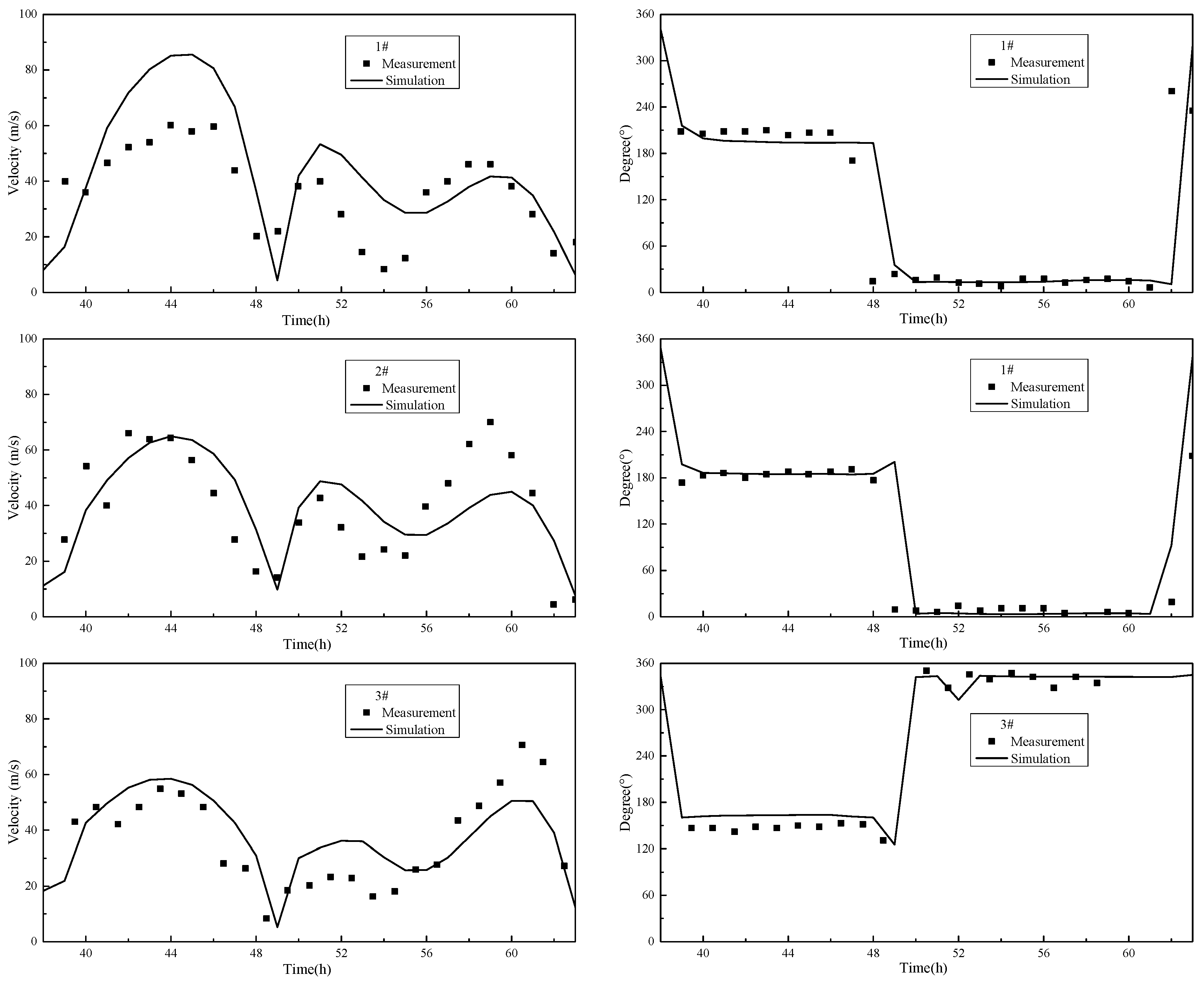
Figure 3.
Comparisons of measured and calculated velocity and direction of neap tides.
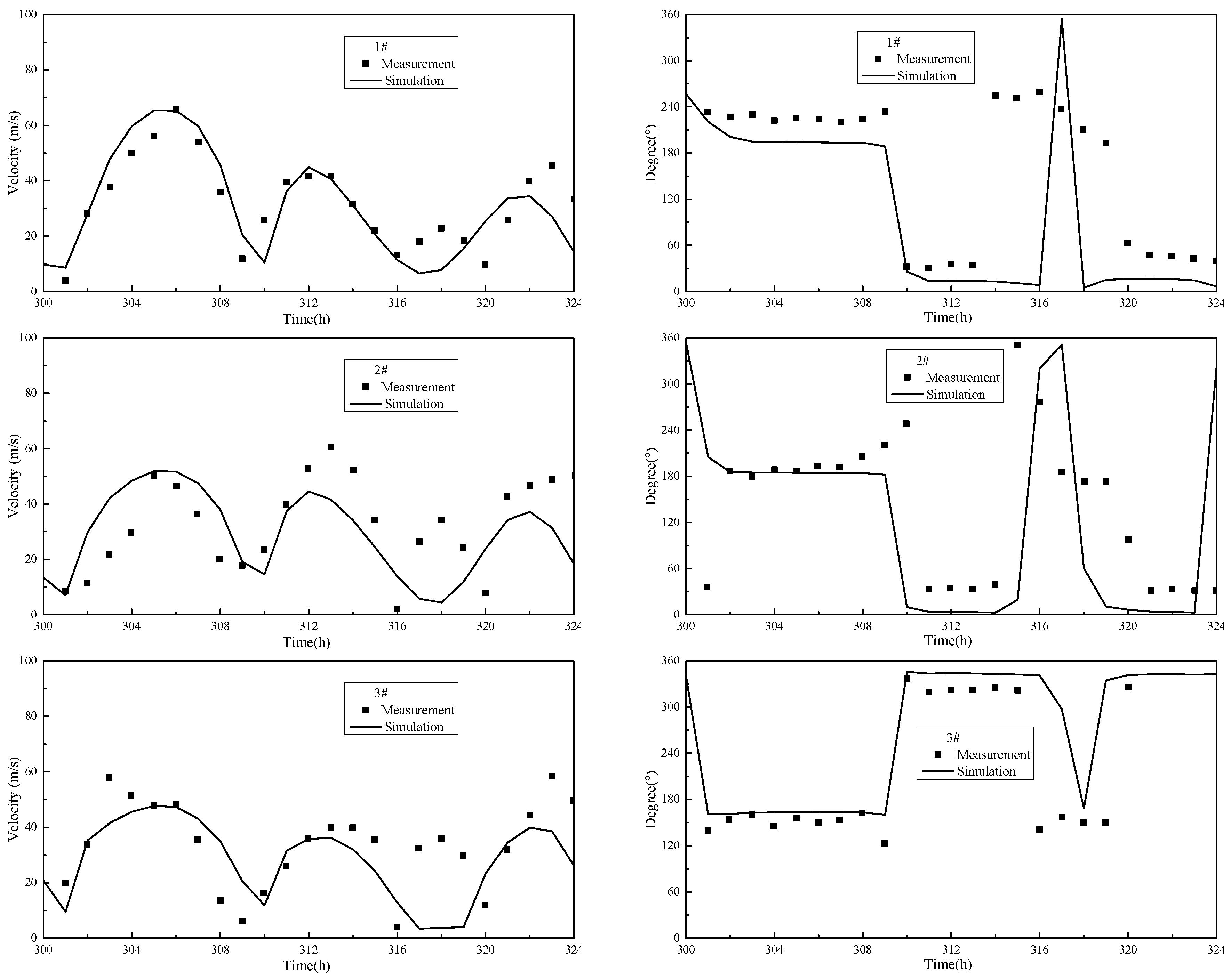
Figure 4.
Comparisons of measured and calculated water levels of (a) spring tides and (b) neap tides.
Figure 4.
Comparisons of measured and calculated water levels of (a) spring tides and (b) neap tides.

Figure 5.
Calculated residence time of different numbers of released particles.

Figure 6.
Spatial distributions of water velocities: (a) ebb current; (c) flood current; and corresponding water depths: (b) ebb current; (d) flood current.
Figure 6.
Spatial distributions of water velocities: (a) ebb current; (c) flood current; and corresponding water depths: (b) ebb current; (d) flood current.

Figure 7.
Map of the streamline of spring and neap tides: (a–d) the tidal process of spring tide (e.g., 4 June 2008); and (e–h) the tidal process of neap tides (e.g., 10 June 2008).
Figure 7.
Map of the streamline of spring and neap tides: (a–d) the tidal process of spring tide (e.g., 4 June 2008); and (e–h) the tidal process of neap tides (e.g., 10 June 2008).
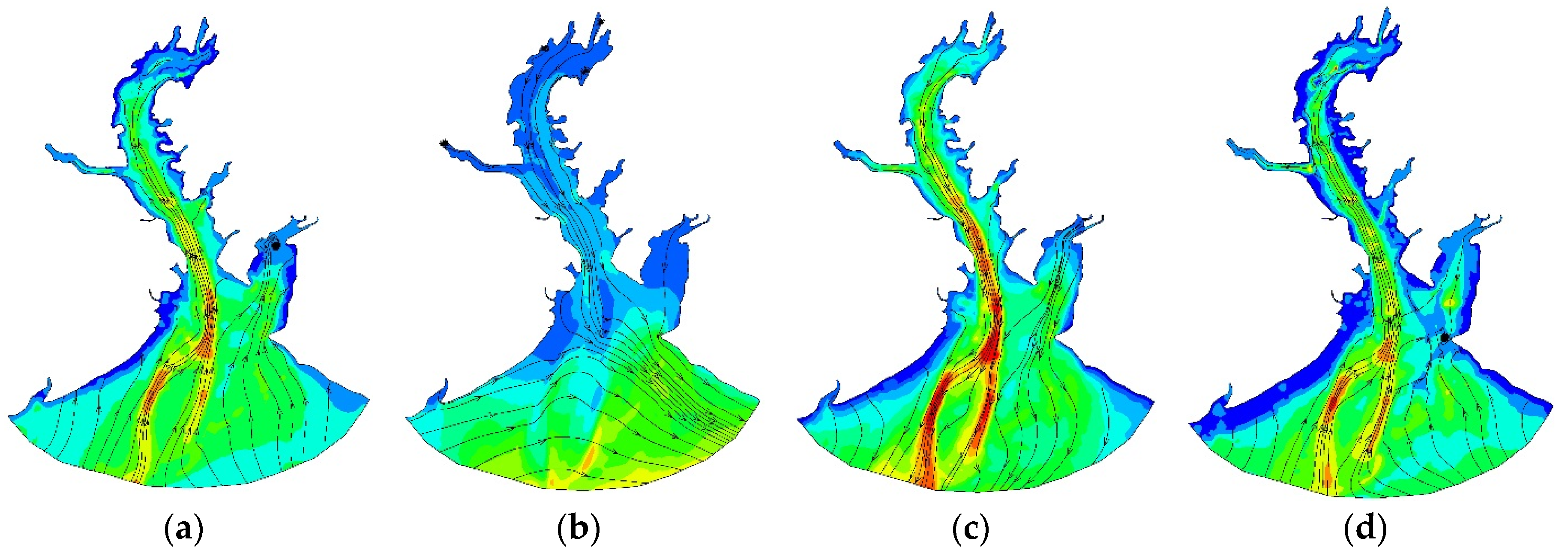
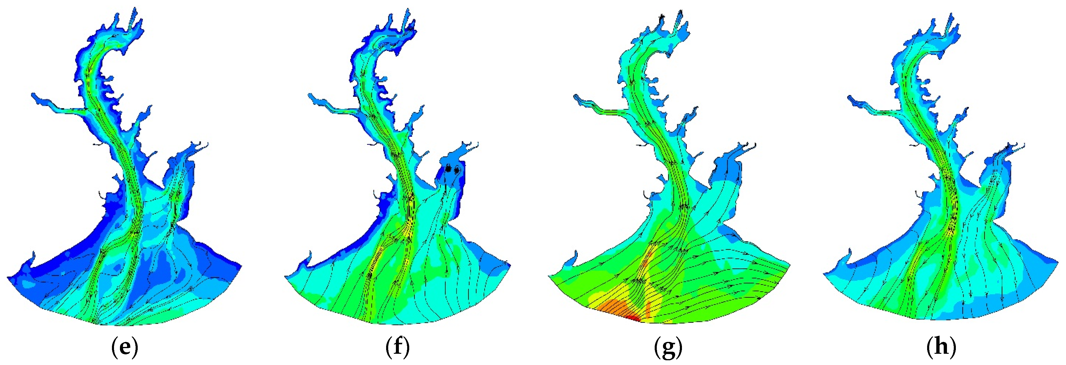
Figure 8.
The number of particles remaining in the bay relative to the initial numbers in summer (2004–2015).
Figure 8.
The number of particles remaining in the bay relative to the initial numbers in summer (2004–2015).
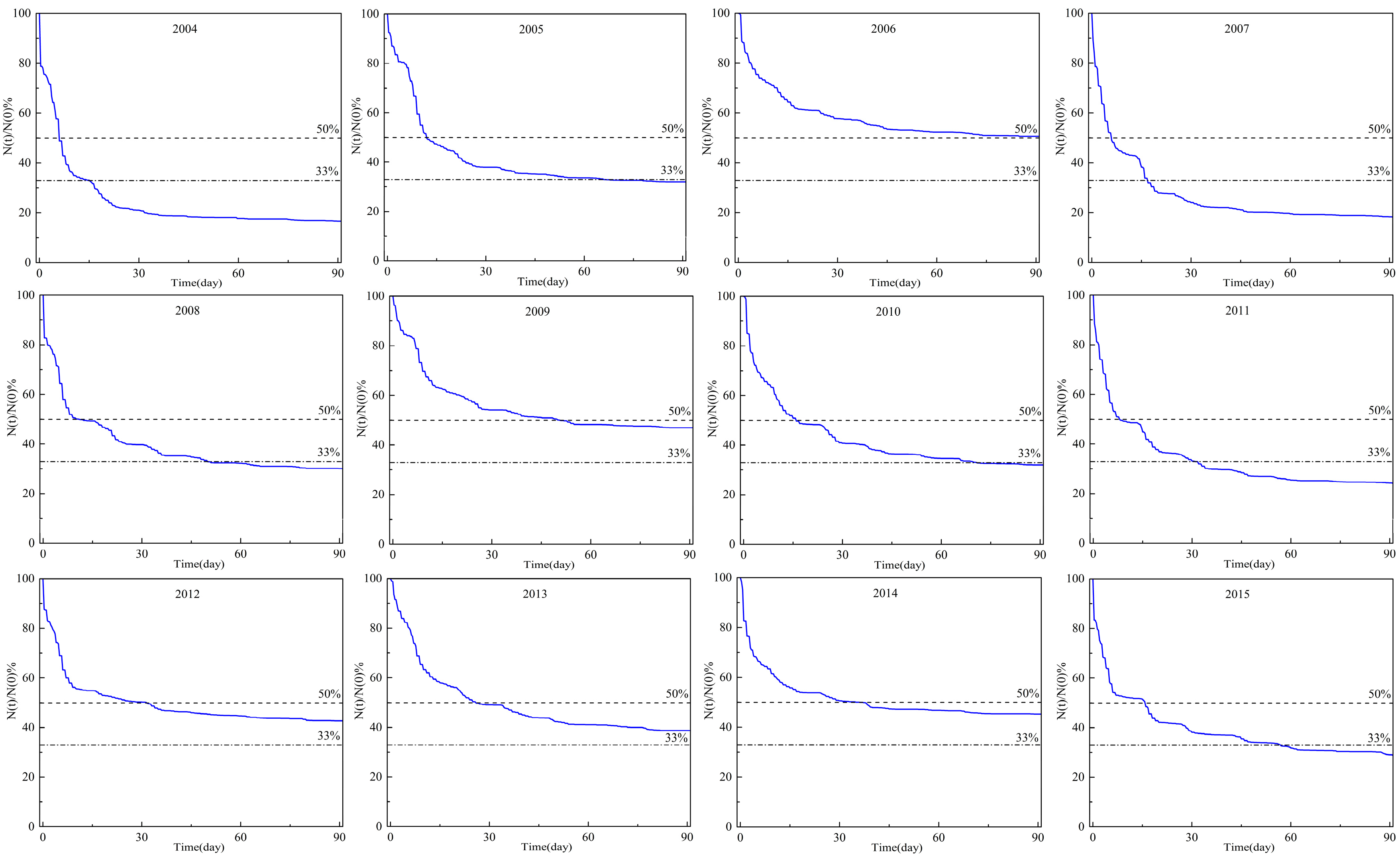
Figure 9.
The number of particles remaining in the bay relative to the initial numbers in winter.

Figure 10.
The residence time when 50% of the initial particles remained in Tieshangang Bay in summer and winter (2004–2015).
Figure 10.
The residence time when 50% of the initial particles remained in Tieshangang Bay in summer and winter (2004–2015).
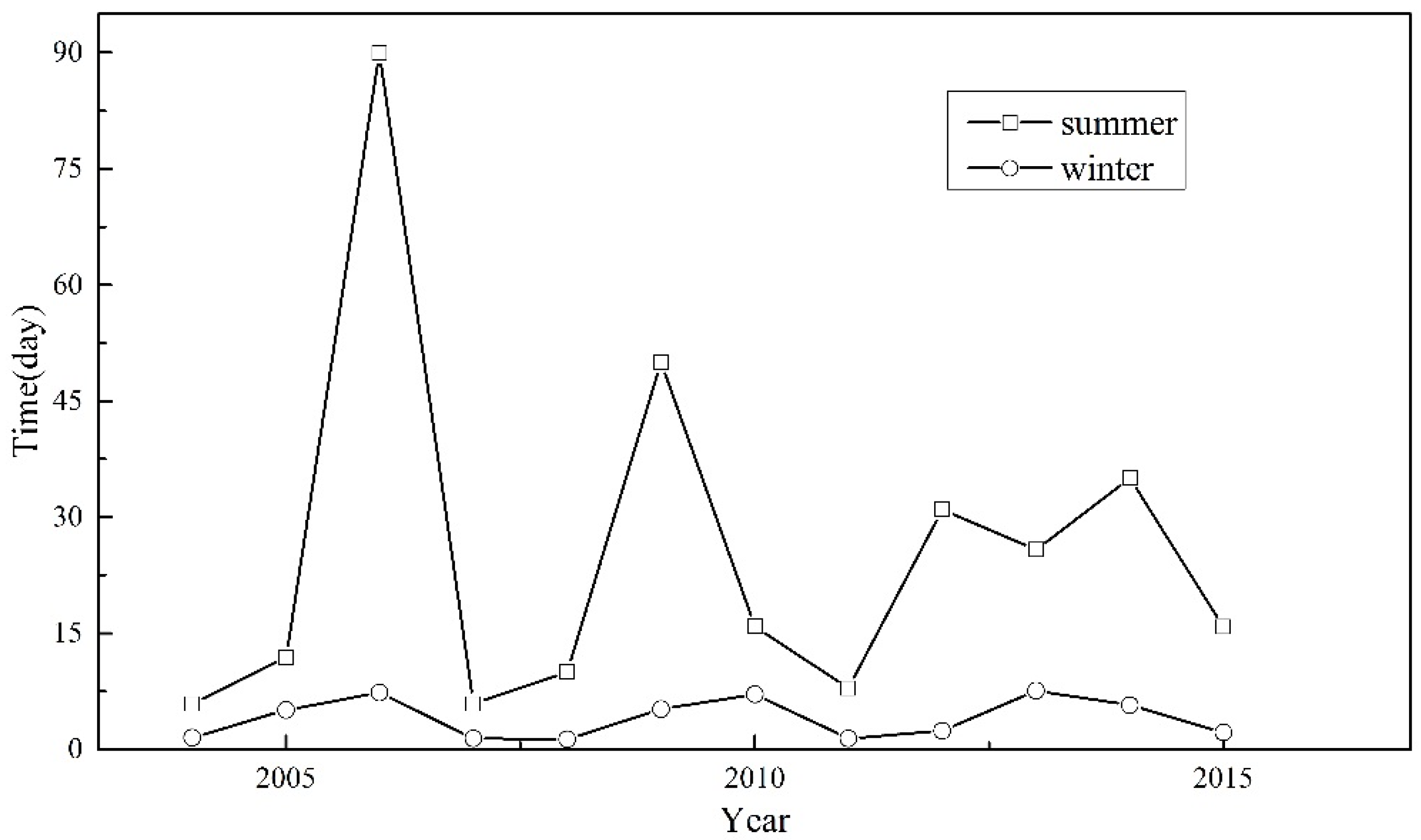
Figure 11.
Spatial distribution of particle trajectories (colored dots) at selected sub-zones during 1 June–1 July 2008. (a–d) represent the particles released at the bay head; (e–h) represent the releases at Shitoubu, the middle of the bay; and (i–l) represent the releases at west trough located at the entrance of the bay.


Figure 12.
Particle distribution after 92-day simulation (a) in summer; (b) in winter (2008).

Table 1.
Different resolution of released particles.
| Case | Numbers | Resolution | 30 Days | 60 Days | 90 Days |
|---|---|---|---|---|---|
| Percentage of Particles | |||||
| 1 | 283 | 2000 m × 1000 m | 39.2% | 36.4% | 32.9% |
| 2 | 534 | 2000 m × 500 m | 38.0% | 33.0% | 29.0% |
| 3 | 934 | 1000 m × 500 m | 32.9% | 29.6% | 27.5% |
| 4 | 1830 | 500 m × 500 m | 32.6% | 28.6% | 26.7% |
| 5 | 4430 | 500 m × 200 m | 31.8% | 27.9% | 26.0% |
Table 2.
Model parameters used for scenario simulations.
| Parameter | Description | Values and Reference |
|---|---|---|
| M | Manning number | 32 m1/3/s [14,15] |
| Ev | Smagorinsky factor for eddy viscosity | 0.28 [20,21,26] |
| Sv | Settling velocity for particles | No settling [26] |
| DV | Vertical dispersion | No dispersion [26] |
| DH | Horizontal dispersion | Scaled eddy viscosity formulation [26] |
Table 3.
The mean residence time (i.e., 33% of the initial particles remaining in the bay) of Tieshangang Bay in summer and winter (2004–2015).
Table 3.
The mean residence time (i.e., 33% of the initial particles remaining in the bay) of Tieshangang Bay in summer and winter (2004–2015).
| Year | 2004 | 2005 | 2006 | 2007 | 2008 | 2009 | 2010 | 2011 | 2012 | 2013 | 2014 | 2015 |
|---|---|---|---|---|---|---|---|---|---|---|---|---|
| Summer | 14.8 | 65.8 | >92 | 16.8 | 49.8 | >92 | 70 | 30.6 | >92 | >92 | >92 | 56.8 |
| Winter | 8.6 | 90 | 57.6 | 24 | 16.3 | 26.8 | 90 | 34.3 | 20 | >92 | 89.8 | 8.8 |
© 2017 by the authors. Licensee MDPI, Basel, Switzerland. This article is an open access article distributed under the terms and conditions of the Creative Commons Attribution (CC BY) license (http://creativecommons.org/licenses/by/4.0/).
Share and Cite
MDPI and ACS Style
Jiang, C.; Liu, Y.; Long, Y.; Wu, C. Estimation of Residence Time and Transport Trajectory in Tieshangang Bay, China. Water 2017, 9, 321. https://doi.org/10.3390/w9050321
AMA Style
Jiang C, Liu Y, Long Y, Wu C. Estimation of Residence Time and Transport Trajectory in Tieshangang Bay, China. Water. 2017; 9(5):321. https://doi.org/10.3390/w9050321
Chicago/Turabian StyleJiang, Changbo, Yizhuang Liu, Yuannan Long, and Changshan Wu. 2017. "Estimation of Residence Time and Transport Trajectory in Tieshangang Bay, China" Water 9, no. 5: 321. https://doi.org/10.3390/w9050321
Note that from the first issue of 2016, this journal uses article numbers instead of page numbers. See further details here.