
Comparative Evaluation of ANN- and SVM-Time Series Models for Predicting Freshwater-Saltwater Interface Fluctuations

1
Korea Institute of Geoscience and Mineral Resources, Daejeon 34132, Korea
2
Jeju Water Resources Headquarters, Jeju 63343, Korea
*
Author to whom correspondence should be addressed.
Water 2017, 9(5), 323; https://doi.org/10.3390/w9050323
Submission received: 21 February 2017
/
Revised: 28 April 2017
/
Accepted: 2 May 2017
/
Published: 4 May 2017
(This article belongs to the Special Issue Groundwater Resources and Salt Water Intrusion in a Changing Environment)
Abstract
:Time series models based on an artificial neural network (ANN) and support vector machine (SVM) were designed to predict the temporal variation of the upper and lower freshwater-saltwater interface level (FSL) at a groundwater observatory on Jeju Island, South Korea. Input variables included past measurement data of tide level (T), rainfall (R), groundwater level (G) and interface level (F). The T-R-G-F type ANN and SVM models were selected as the best performance model for the direct prediction of the upper and lower FSL, respectively. The recursive prediction ability of the T-R-G type SVM model was best for both upper and lower FSL. The average values of the performance criteria and the analysis of error ratio of recursive prediction to direct prediction (RP-DP ratio) show that the SVM-based time series model of the FSL prediction is more accurate and stable than the ANN at the study site.
1. Introduction
Monitoring and forecasting of temporal changes of the freshwater-saltwater interface level (FSL) in coastal areas is necessary for the early detection of saltwater intrusion and the management of coastal aquifers. To measure the location and variation of FSL, the geophysical well logging technique to capture the vertical profile of electrical conductivity or salinity has been traditionally employed [1,2]. Recently, research has been conducted on the development of an interface egg device to monitor the temporal variation of FSL [3].
For the simulation or prediction of saltwater intrusion into aquifers, physics-based numerical models have been developed and applied to various field sites; Gingerich and Voss [4] applied 3D-SUTRA model to a coastal aquifer in Hawaii for the simulation of the saltwater intrusion; Werner and Gallagher [5] characterized seawater intrusion in coastal aquifers of the Pioneer Valley, Australia using MODHMS model; Guo and Langevin [6] developed SEAWAT, a variable-density finite-difference groundwater flow mode and Rozell and Wong [7] applied it to Shelter Island, USA for assessing effects of climate change on the groundwater resources; Yechieli et al. [8] examined the response of the Mediterranean and Dead Sea coastal aquifers using FEFLOW model. Physics-based numerical models are powerful tools for the simulation or prediction of temporal and spatial variation of FSL in a given domain. However, they require a large quantity of precise data related to the physical properties of the domain, a lack of which can cause severe deterioration in the accuracy and reliability of their results [9,10]. Time series modeling can be an effective alternative approach for predicting saltwater intrusion where geological and geophysical surveys are limited and monitoring data of temporal variation related to saltwater intrusion are available.
Recently, in the field of hydrology and hydrogeology, research on the application of time series models—based on machine learning techniques such as an artificial neural network (ANN) and a support vector machine (SVM) to prediction of water resources variations—have been increased; Zealand et al. [11] utilized the ANN for forecasting short term stream flow of the Winnipeg River system in Canada; Akhtar et al. [12] applied ANN to river flow forecasting at Ganges river; Hu et al. [13] explored new measures for improving the generalization ability of the ANN for the prediction of the rainfall-runoff; Coulibaly et al. [14] and Mohanty et al. [15] examined the performance of ANN for the prediction of groundwater level (GWL) fluctuations; Coppola et al. [16] used the ANN for the prediction of GWL under variable pumping conditions; Liong and Sivapragasam [17], and Yu et al. [18] employed the SVM for the prediction of the flood stage; Asefa et al. [19] used the SVM for designing GWL monitoring networks; Gill et al. [20] assessed the effect of missing data on the performance of ANN and SVM models for GWL prediction; Yoon et al. [21] used ANN and SVM for long-term GWL forecast.
For coastal aquifer management, time series models have been developed to predict groundwater level (GWL) fluctuations using machine learning methods [22,23,24]. In the domain of saltwater intrusion, recent studies have used a time series modeling approach [25,26]; however, their target was to predict salinity at coastal rivers rather than FSL change in coastal aquifers.
In this study, we monitored temporal variations of the upper and lower FSL of a groundwater observatory at Jeju Island in South Korea. Using the observed FSL data, we designed time series models based on artificial neural networks and support vector machines for the prediction of FSL fluctuations. The prediction accuracy of FSL was estimated with different structures of models. The paper is organized as follows: Section 2 describes the study site and FSL monitoring data. Section 3 describes the development of the time series models for FSL prediction based on artificial neural networks and the support vector machines. The FSL prediction results are described and discussed in Section 4, and conclusions are drawn in Section 5.
2. FSL Monitoring
2.1. Study Area
The study site is a groundwater observatory (HD2) located at the north-eastern part of Jeju Island in South Korea (Figure 1). Jeju Island is the largest volcanic island in South Korea with an area of 1849 km2, where the mean annual air temperature is 16.2 °C and total annual precipitation is 1710 mm.
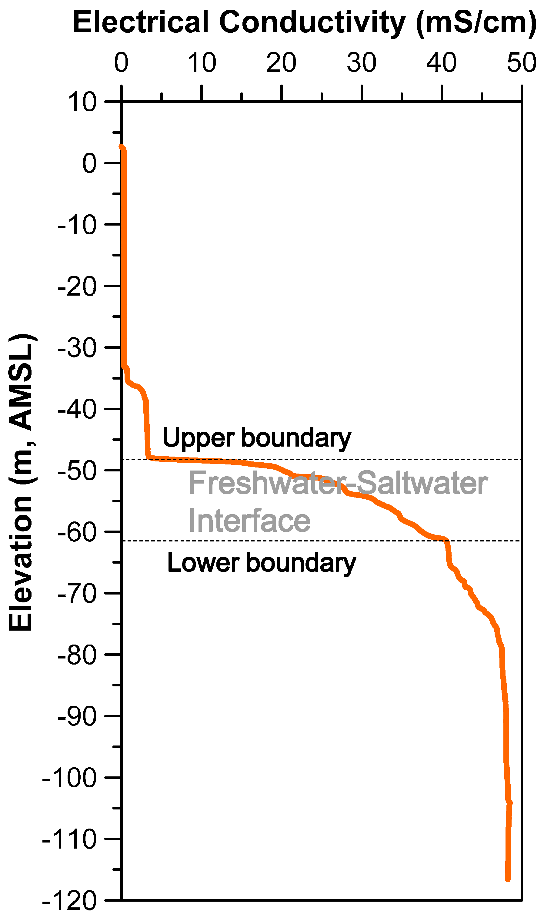
Perennial rivers are scarce on Jeju Island, so groundwater is a main water source for domestic, agricultural or industrial uses, as well as a main source of drinking water, therefore, the groundwater has been systematically managed with a saltwater intrusion monitoring network by the local government. The HD2 groundwater observatory (one of the saltwater intrusion monitoring networks), is located 2.3 km from the coast-line and 42.73 m (above mean sea level: AMSL). Rainfall and tide level monitoring stations are located near the north-eastern shoreline at a distance of 6.1 km and 12.3 km from HD2, respectively. A geophysical survey was conducted to measure the vertical profile of electrical conductivity in HD2. The results show that the freshwater-saltwater interface appears between −49.0 m and −62.0 m (AMSL) where the electrical conductivities are 16.2 mS/cm and 40.7 mS/cm, respectively (Figure 2).
2.2. Monitoring Device and Data
We utilized the interface egg developed by Kim et al. [3] to monitor the temporal variation of FSL at the HD2 observatory. The interface egg is a monitoring probe designed to have a specific density of the value between freshwater and saltwater, which enables it to float on the FSL based on the concept of neutral buoyancy. Using the measured pressure data of the interface egg, and a pressure sensor at a fixed depth, the position of the FSL at time t is estimated as follows (Figure 3):
where EL is an elevation of a top of well casing; a(t) is the pressure value measured at fixed depth b; and c(t) is the pressure value measured at the interface egg.
FSL(t) = EL − (b − a(t) + c(t))
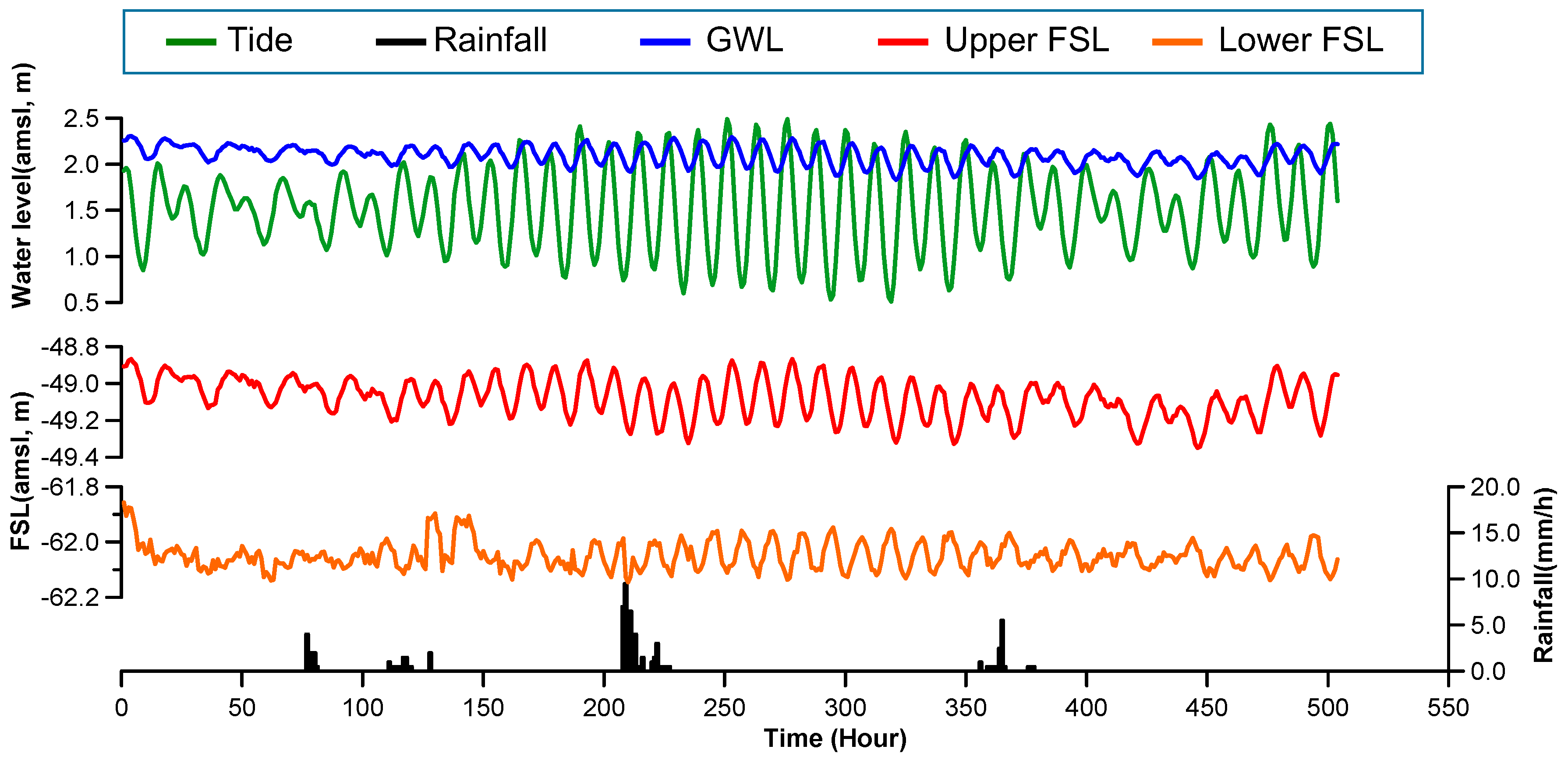
Taking into account the vertical profile of electrical conductivity, we installed two interface eggs at around −49.0 m and −62.0 m (AMSL) which corresponded to the upper and lower boundaries of the freshwater-saltwater interface at the HD2 observatory. We additionally installed a pressure sensor at a fixed depth to monitor the GWL fluctuations. Hourly measured data of GWL, upper and lower FSLs, rainfall and tide level from 15 September–5 October 2014, are shown in Figure 4.
The result of cross correlation analyses between the time series data at the HD2 observatory shows that the correlation of upper FSL with tide and GWL is much higher than of the lower FSL (Table 1). The maximum correlation coefficient between GWL and upper FSL is the highest: 0.97 at a lag time of 0 h, which indicates that the movement of the upper FSL is strongly and immediately influenced by GWL. Furthermore, the maximum correlation coefficient of tide–GWL and tide–upper FSL are as high as 0.85 and 0.83 at a lag time of 2 h, respectively. The correlation of rainfall with GWL and FSL is not significant for this study.
3. FSL Prediction Model Development
We employed artificial neural network (ANN) and support vector machine (SVM) techniques to construct time series models for the prediction of the upper and lower FSL fluctuations. Theoretical backgrounds of the ANN, SVM, and time series modeling process are described below.
3.1. Aritificial Neural Network (ANN)
The ANN is a mathematical framework patterned after the parallel processing sequence of the human brain. A feedforward network (FFN), one of the most common structures of the ANN, is generally composed of three layers of input, hidden and output (Figure 5a). Each layer of the ANN has a certain number of nodes and each node in a layer is connected to other nodes in the next layer with a specific weight and bias. The mathematical expression of the calculation process in the FFN is as follows:
where the subscript i and j denote the previous and present layer, respectively; is the nodal value; and are weight and bias values, respectively; is the number of nodes in the previous layer; and denotes a transfer function of the present layer. Log-sigmoid and linear functions were allocated to hidden and output layers, respectively, which are known to be an effective combination for enhancing the extrapolation ability of the ANN [27,28].
The purpose of the ANN model building is to find the optimal values of weights and biases by learning or training from the given input and output data. We employed a back-propagation algorithm (BPA) with momentum suggested by Rumelhart and McClelland [29] for training the ANN. The weight and bias update rule of the BPA can be expressed as follows:
where is a sum of squared errors between observed () and estimated () values at n-th weight and bias update stage, MM and LR denote the momentum and learning rate values, respectively, and N is the number of data allocated to the training stage. In this study, three model parameters; i.e., number of hidden nodes (HN), MM and LR were determined by a grid search that is one of the trial and error method. We took into account 6 values for every ANN model parameters: HN ∈ [2, 5, 10, 15, 20, 25], MM ∈ [0.0, 0.1, 0.3, 0.5, 0.7, 0.9], and LR ∈ [0.001, 0.005, 0.01, 0.015, 0.02, 0.025], which composes 216 candidate groups of model parameters.
3.2. Suport Vector Machine (SVM)
The SVM, a relatively new machine learning method suggested by Vapnik [30], is based on the structural risk minimization (SRM) rather than the empirical risk minimization (ERM) of the ANN. From a data classification point of view, ERM based machine learning method is designed to minimize the error of the estimated classifier for the data in the training stage. Therefore, the model update is stopped when the error of the training stage data is zero or within a certain value of the tolerance. The SRM based method, such as the SVM, is designed to maximize a margin between data groups to be classified, which maximize the generalization ability of the model. The mathematical expression of the output estimation of the SVM is as follows:
where S denotes an SVM estimator, denotes a weight vector, is a nonlinear transfer function that maps input vectors into a higher-dimensional feature space. Platt [31] introduced a convex optimization problem with an -insensitivity loss function to find the solution of Equation (6) as follows:
where and are slack variables that penalize errors of estimated values over the error tolerance , C is a trade-off parameter that controls the degree of the empirical error in the model building process, and is the input vector in the training stage. Equation (7) can be solved using Lagrangian multipliers and the Karush-Kuhn-Tucker (KKT) optimality condition as follows:
where and are Lagrangian multipliers, K is a kernel function defined by an inner product of the nonlinear transfer functions. A radial basis function with parameter is commonly used as the kernel function:
We employed the sequential minimal optimization (SMO) algorithm [32] to solve Equation (8) and construct the SVM model. The SMO minimizes a subset of target variables by two and finds an analytical solution of the subset repeatedly, until all given input vectors satisfy the KKT conditions. A detailed explanation of the SMO algorithm can be found in References [31,32]. The SVM model parameters of C, , and were selected by the grid search method like the ANN. We took into account six values for every SVM model parameters: C ∈ [0.5, 1.0, 3.0, 5.0, 7.0, 10.0], ∈ [0.01, 0.05, 0.1, 0.11, 0.12, 0.13], and ∈ [0.5, 1.0, 1.5, 2.0, 2.5, 3.0], which composes 216 candidate combinations of model parameters. A schematic diagram of the SVM structure is shown in Figure 5b.
3.3. Time Series Modeling Strategy
In general, two types of strategies can be taken into account for time series modeling: direct and recursive prediction [33,34]. The direct prediction strategy always uses actual measured data as input components, thus, model accuracy is high, especially for short-term predictions. For long-term predictions, it requires separate models for every prediction horizon, which increases the computational burden and reduces the efficiency of the time series modeling. The direct prediction strategy can be expressed as follows:
where is estimated target value at time t based on the direct prediction strategy, is a time series model of the direct prediction for the prediction horizon of h; and are i-th exogenous input variable and its components, respectively; is an autoregressive input variable that is identical to a target variable; and are the number of past measurement data for and . The autoregressive input variable can be deleted if a model only uses exogenous inputs.
The recursive prediction strategy generally utilizes 1-lead time ahead of the direct prediction model repeatedly for estimating the autoregressive input components, which enables the model to perform a simulation and long-term prediction effectively. However, the error occurred from the direct prediction model in the previous time step can be accumulated continuously with time steps, which can deteriorate the model performance significantly [21,34]. Therefore, it is important to build an adequate direct prediction model for stable and accurate recursive prediction. The recursive prediction strategy is expressed as:
where is estimated target value at time t based on the recursive prediction strategy, is a 1-lead time direct prediction model and is the estimated autoregressive input variable. In this study, ANN- and SVM-based time series models with four types of input structures as combinations of tide level, rainfall, GWL, and FSL were designed for upper and lower FSL data, respectively. The number of past measurement data used for the component of each variable is described in Table 2. As an example, estimated upper FSL value at time t based on the 1-lead time ahead of direct and recursive prediction strategies using T-R-G-F type model can be expressed as Equations (12) and (13), respectively.
where and are measured data of tide, rainfall, and GWL at time t-k, respectively; and are measured and estimated FSL values at time t, respectively.
The data allocation for the model building and validation stages of the ANN and SVM models are described in Table 3.
4. Results and Discussion
4.1. Direct Prediction of FSL
Time series models of 1-h direct prediction for the upper and lower FSL were constructed. The selected model parameters of the ANN and SVM for each type of input structure are described in Table 4.
Three performance criteria were used to evaluate the prediction ability of the ANN and SVM model, including the root mean squared error (RMSE), mean absolute relative error (MARE), and correlation coefficient (CORR), as follows:
where and denote the maximum and minimum values of the observed data, respectively; and and denote the average observed and estimated values, respectively. The RMSE is a useful index for model performance evaluation when large errors are particularly undesirable as the errors are squared before they are averaged, which makes large errors have a relatively high weight. The MARE is the mean absolute error value divided by the range of observed data, thus it can compare the prediction results of the time series data showing different ranges of fluctuation. The CORR measures the extent and direction of a linear relationship between the observed and estimated values.
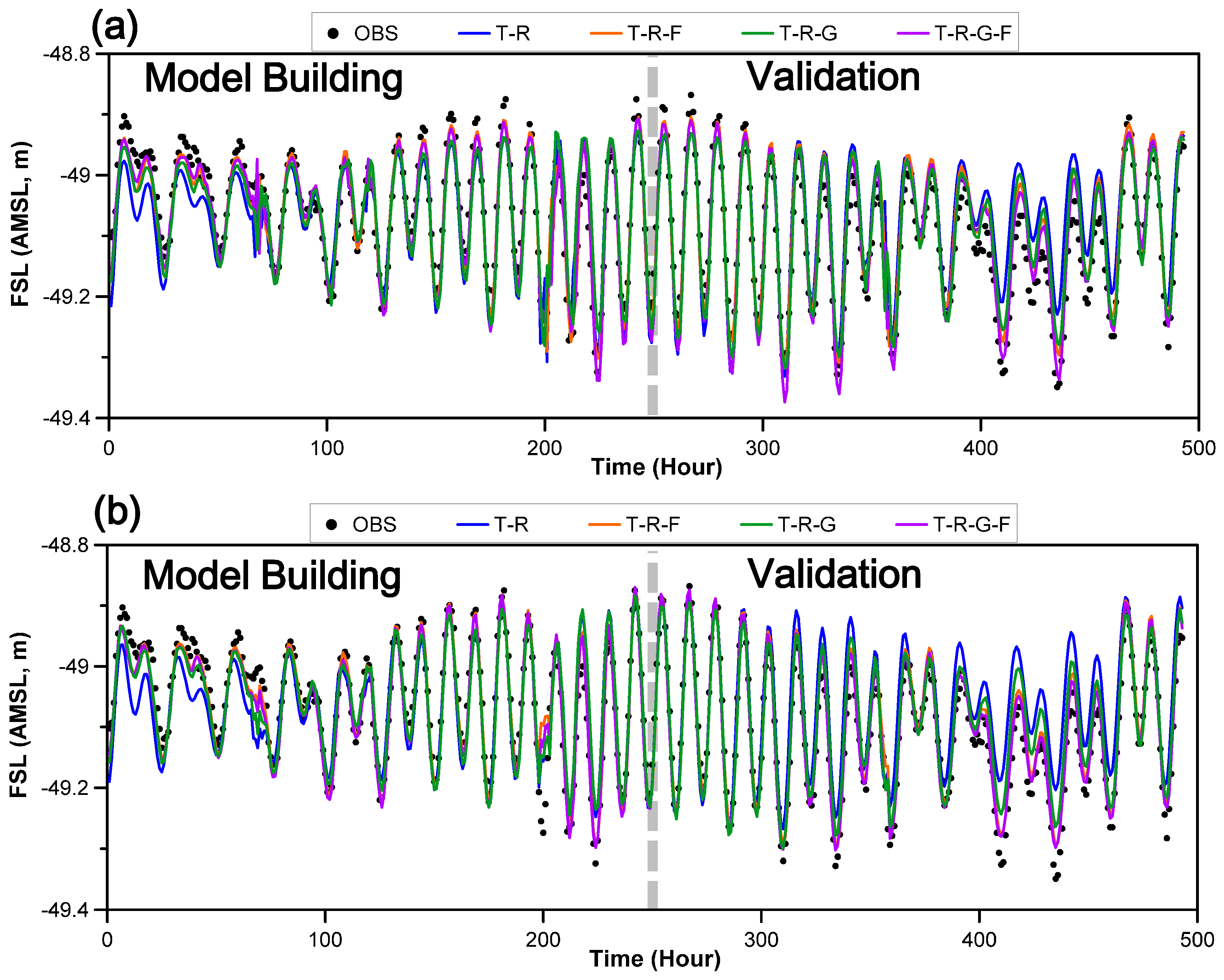
The model performance criteria of ANN and SVM models for 1-h direct prediction of the upper FSL show that overall prediction accuracy is high: RMSE was below 0.07 m, MARE below 10.82%, and CORR over 0.89 (Table 5). The model performance of the T-R-F and T-R-G-F type models (which uses past measurement data of FSL as input values) were better than that of the T-R and T-R-G type models. The T-R-G-F type SVM model showed the best performance for 1-h direct prediction of the upper FSL. The average value of each performance criteria shows that the overall direct prediction ability of the SVM was better than ANN for the upper FSL data in this study. The observed data and direct prediction results for the upper FSL are shown in Figure 6. Various types of ANN and SVM models were trained adequately during the model building stage and there was no significant difference between the estimated values for the input structures.
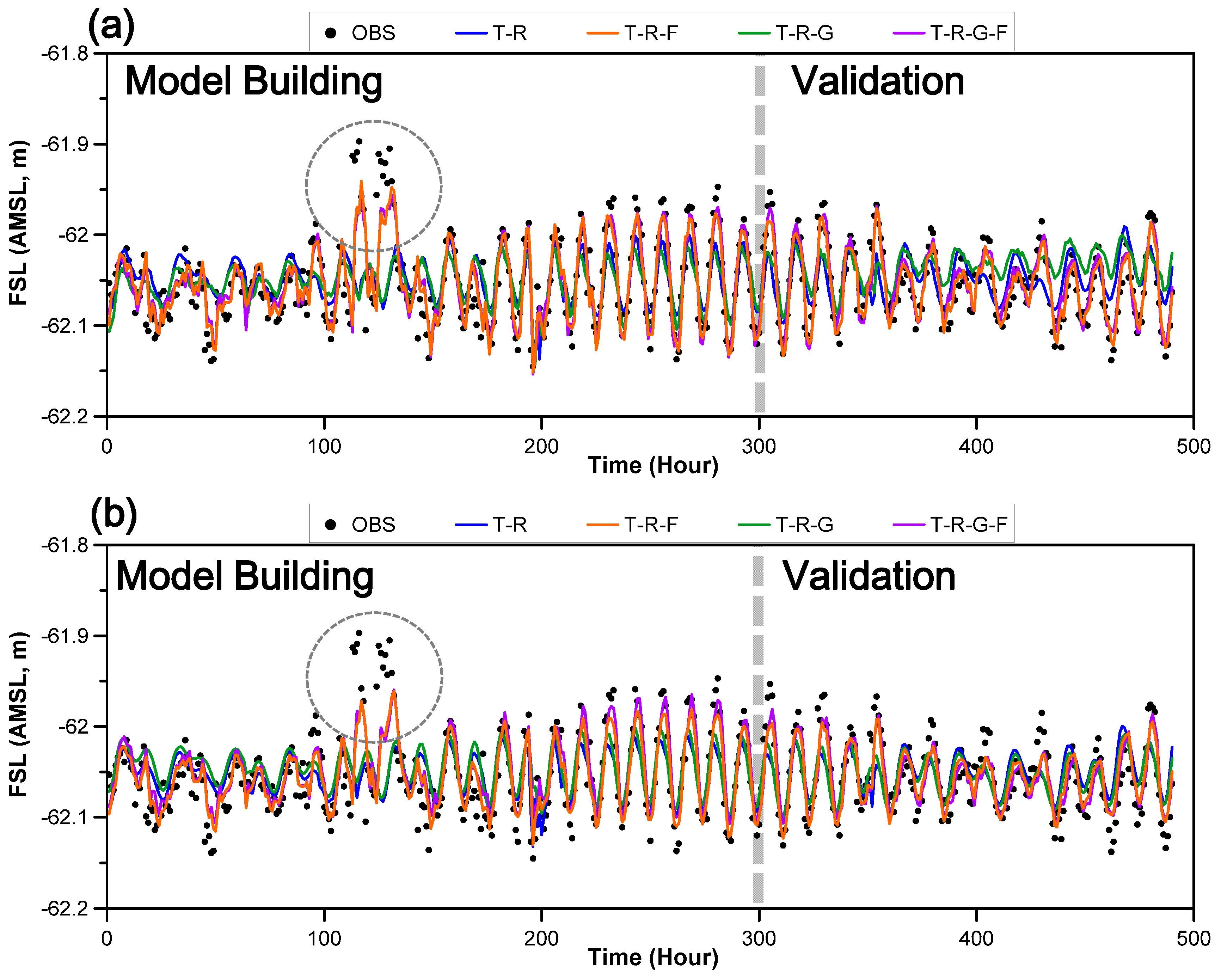
The quality performance of the direct prediction for the lower FSL was not as high as the upper FSL: the MARE values lay between 8.438% and 18.494%, and CORR values between 0.549 and 0.908 (Table 6). The RMSE values, ranging from 0.020 m to 0.040 m, were lower than the upper FSL prediction; however, this was not due to the prediction result for the lower FSL being better, but that the range of fluctuation of the lower FSL was smaller than the upper. The correlation of tide level and GWL with the lower FSL was weaker than the correlation with the upper FSL, which could cause deterioration in the model performance. The performance of the T-R-F and T-R-G-F type models was better than that of the T-R and T-R-G type models for lower FSL prediction, which was similar to the upper FSL prediction. The T-R-G-F type ANN model showed the best performance for 1-h direct prediction of the lower FSL; however, the average value of the performance criteria of the SVM models was better than the ANN. The observed data and direct prediction results for the lower FSL are shown in Figure 7. The model building stage data included some abnormally high peaks (dashed circle) that probably had occurred due to pumping for an agricultural activity around the study site, which were not sufficiently trained by the ANN and SVM models, and can cause the underestimation at peak values in the validation stage.
The results of the direct prediction showed that the best performance models for the upper and lower FSL were different and that the performance of the SVM model was less sensitive to the input structure of the ANN for the FSL data.
4.2. Recursive Prediction of FSL
The recursive prediction models of the upper and lower FSL were designed using the 1-h direct prediction models. The model performance criteria for the recursive prediction of the upper and lower FSL are described in Table 7 and Table 8, respectively.
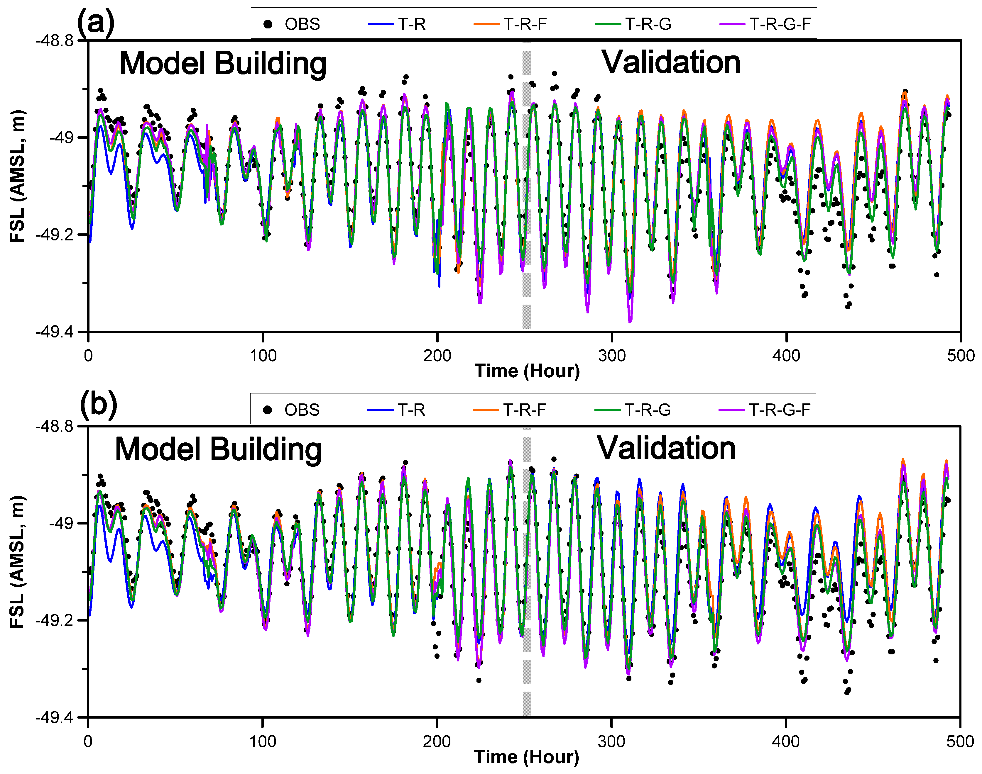
The overall model performance of the recursive prediction was lower than the direct prediction. The T-R-G type SVM models showed the best performance and the average values of the performance criteria of the SVM was superior to ANN for the recursive prediction of both the upper and lower FSL. The success of the recursive prediction highly relied on the generalization ability of the model to capture the relationship between the input and output variables of the given system as the observed data of the output variables are not available as input components. Based on the SRM, the inherent generalization ability of the SVM may capture the relationship between input and output data of this study more effectively than the ANN. The recursive prediction results of the ANN and SVM models for the upper and lower FSL are shown in Figure 8 and Figure 9, respectively.
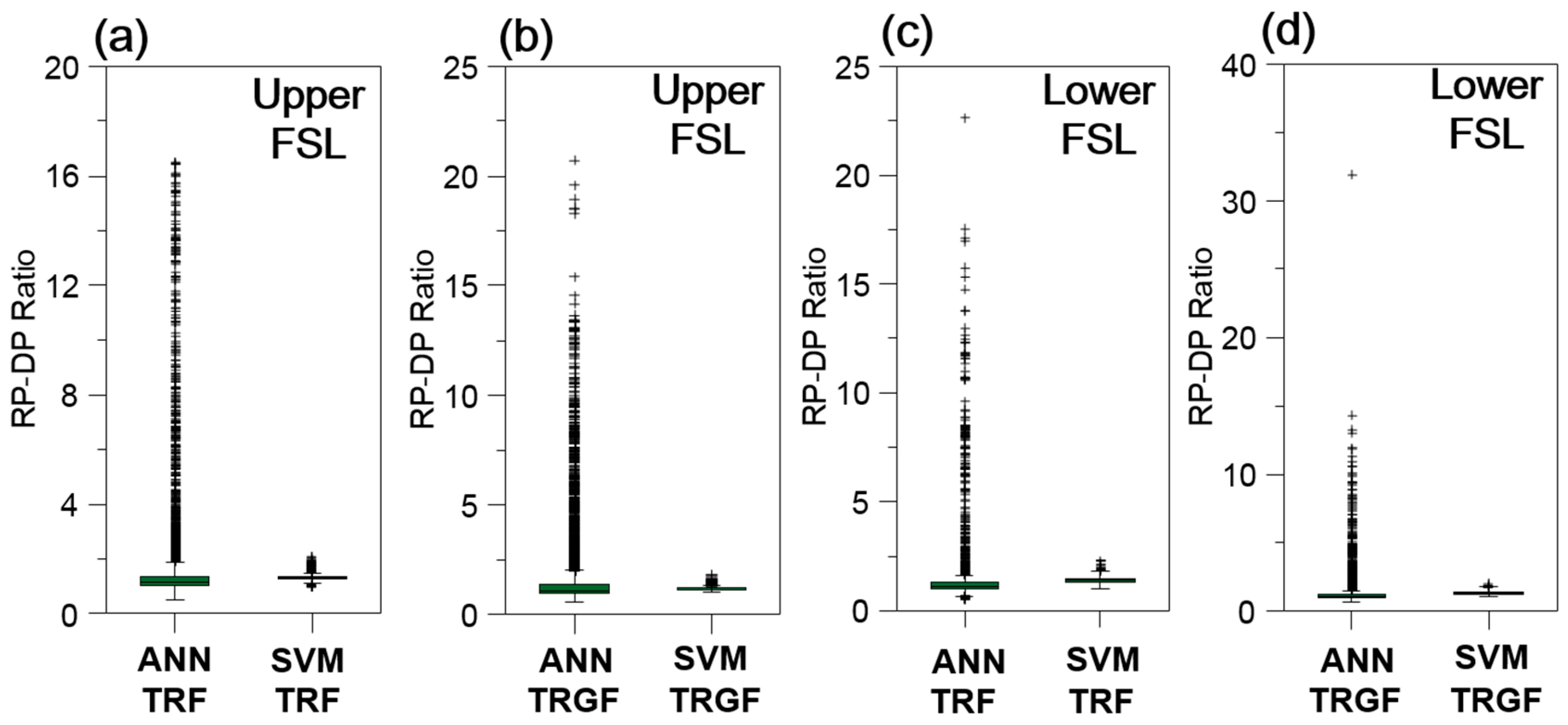
The direct prediction strategy is efficient for the short-term prediction where a real-time measurement data of the target variable is available, and the recursive prediction strategy is necessary for the long-term prediction or the simulation of the target variable variation. However, as mentioned above and in Section 3.3, the error of the estimated target value can be accumulated with time steps in the recursive prediction strategy. Thus, it is important to build an adequate direct prediction model that learnt a response function of the given system. To evaluate the stability of the recursive model building, the RP-DP ratio [24] was calculated for T-R-F and T-R-G-F type models with 216 candidate model parameter groups:
The RP-DP ratio value stands for the extent of the consistency between the direct and recursive prediction models. Thus, a narrower distribution with lower values of the RP-DP ratio indicates a higher possibility that a recursive prediction model of high consistency with a direct prediction model is selected. The calculated RP-DP ratio values of the ANN models were more distributed than the SVM for both the T-R-F and T-R-G-F type models and the upper and lower FSL (Figure 10). These results indicate that the SVM method is more efficient and stable than the ANN for the recursive prediction of the FSL data in this study.
5. Summary and Conclusions
In this study, the temporal variation of the upper and lower FSL was monitored using interface eggs at the HD2 observatory on Jeju Island, South Korea. The ANN- and SVM-based time series models of FSL prediction were developed and their performance compared. The result of the direct prediction shows that the T-R-G-F type ANN model was best for upper FSL prediction and the T-R-G-F type SVM model for the lower FSL. The T-R-G type SVM model was best for the recursive prediction of both upper and lower FSL. The average values of the model performance criteria indicated that the overall prediction ability of the SVM model was superior to the ANN. The analysis of the RP-DP ratio distribution showed that the SVM-based recursive prediction model was more stable and efficient than the ANN for FSL prediction of the study site.
The monitoring and prediction of FSL is necessary for the sustainable use of groundwater resources in coastal aquifers. The groundwater is the sole and main water source of Jeju Island and the local government has installed and operated a saltwater intrusion monitoring network. It is expected that the developed model for FSL prediction can be a useful tool in the future management of groundwater resources in coastal areas.
Acknowledgments
This research was supported by Korea Ministry of Environment as “GAIA (Geo-Advanced Innovative Action) Project (#2016000530004)”.
Author Contributions
Heesung Yoon and Kyoochul Ha designed and performed numerical experiments and wrote the paper; Yongcheol Kim and Soo-Hyung Lee set the monitoring system and conducted the time series analysis; Gee-Pyo Kim measured the vertical profile of the electrical conductivity at the study site.
Conflicts of Interest
The authors declare no conflicts of interest.
References
- Kim, K.; Seong, H.; Kim, T.; Park, K.; Woo, N.; Park, Y.; Koh, G.; Park, W. Tidal effects on variations of fresh-saltwater interface and groundwater flow in a multilayered coastal aquifer on a volcanic island (Jeju Island, Korea). J. Hydrol. 2006, 330, 525–542. [Google Scholar] [CrossRef]
- Liu, C.K.; Dai, J.J. Seawater intrusion and sustainable yield of basal aquifers. J. Am. Water Resour. Assoc. 2012, 48, 861–870. [Google Scholar] [CrossRef]
- Kim, Y.; Yoon, H.; Kim, K.P. Development of a novel method to monitor the temporal change in the location of the freshwater-saltwater interface and time series models for the prediction of the interface. Environ. Earth Sci. 2016, 75, 882–891. [Google Scholar] [CrossRef]
- Gingerich, S.B.; Voss, C.I. Thee-dimensional variable-density flow simulation of a coastal aquifer in southern Oahu, Hawaii, USA. Hydrogeol. J. 2005, 13, 436–450. [Google Scholar] [CrossRef]
- Wener, A.D.; Gallagher, M.R. Characterization of sea-water intrusion in the Pioneer Valley, Australia using hydrochemistry and three-dimensional numerical modelling. Hydrogeol. J. 2006, 14, 1452–1469. [Google Scholar] [CrossRef]
- Guo, W.; Langevin, C.D. User’s Guide to SEWAT: A Computer Program for Simulation of Three-Dimensional Variable-Density Ground-Water Flow; United States Geological Survey: Tallahassee, FL, USA, 2002; p. 73.
- Rozell, D.J.; Wong, T. Effects of climate change on groundwater resources at Shelter Island, New York State, USA. Hydrogeol. J. 2010, 18, 1657–1665. [Google Scholar] [CrossRef]
- Yechieli, Y.; Shalev, E.; Wollman, S.; Kiro, Y.; Kafri, U. Response of the Mediterranean and Dead Sea coastal aquifers to sea level variations. Water Resour. Res. 2010, 46, W12550. [Google Scholar] [CrossRef]
- Bardossy, A. Calibration of hydrological model parameters for ungauged catchments. Hydrol. Earth Syst. Sci. 2007, 11, 703–710. [Google Scholar] [CrossRef]
- Pollacco, J.A.P.; Ugalde, J.M.S.; Angulo-Jaramillo, R.; Braud, I.; Saugier, B. A linking test to reduce the number of hydraulic parameters necessary to simulate groundwater recharge in unsaturated zone. Adv. Water Resour. 2008, 31, 355–369. [Google Scholar] [CrossRef]
- Zealand, C.M.; Burn, D.H.; Simonovic, S.P. Short-term streamflow forecasting using artificial neural networks. J. Hydrol. 1999, 214, 32–48. [Google Scholar] [CrossRef]
- Akhtar, M.K.; Corzo, G.A.; van Andel, S.J.; Jonoski, A. River flow forecasting with artificial neural networks using satellite observed precipitation pre-processed with flow length and travel time information: Case study of the Ganges river basin. Hydrol. Earth Syst. Sci. 2009, 13, 1607–1618. [Google Scholar] [CrossRef]
- Hu, T.S.; Lam, K.C.; Ng, S.T. A modified neural network for improving river flow prediction. Hydrol. Sci. J. 2005, 50, 299–318. [Google Scholar] [CrossRef]
- Coulibaly, P.; Anctil, F.; Aravena, R.; Bobee, B. Artificial neural network modeling of water table depth fluctuations. Water Resour. Res. 2001, 37, 885–896. [Google Scholar] [CrossRef]
- Coppola, E.; Rana, A.J.; Poulton, M.M.; Szidarovszky, F.; Uhl, V.V. A neural network model for predicting aquifer water level elevations. Groundwater 2005, 43, 231–241. [Google Scholar] [CrossRef] [PubMed]
- Mohanty, S.; Jha, M.K.; Kumar, A.; Sudheer, K.P. Artificial neural network modeling for groundwater level forecasting in a river island of eastern India. Water Resour. Manag. 2010, 24, 1845–1865. [Google Scholar] [CrossRef]
- Liong, S.Y.; Sivapragasam, C. Flood stage forecasting with support vector machines. J. Am. Water Resour. Assoc. 2002, 38, 173–186. [Google Scholar] [CrossRef]
- Yu, P.S.; Chen, S.T.; Chang, I.F. Support vector regression for real-time flood stage forecasting. J. Hydrol. 2006, 328, 704–716. [Google Scholar] [CrossRef]
- Asefa, T.; Kemblowski, M.W.; Urroz, G.; McKee, M.; Khalil, A. Support vectors-based groundwater head observation networks design. Water Resour. Res. 2004, 40, W1150901. [Google Scholar] [CrossRef]
- Gill, M.K.; Asefa, T.; Kaheil, Y.; McKee, M. Effect of missing data on performance of learning algorithms for hydrologic prediction: Implication to an imputation technique. Water Resour. Res. 2007, 43, W07416. [Google Scholar] [CrossRef]
- Yoon, H.; Hyun, Y.; Ha, K.; Lee, K.K.; Kim, G.B. A method to improve the stability and accuracy of ANN- and SVM-based time series models for long-term groundwater level predictions. Comput. Geosci. 2016, 90, 144–155. [Google Scholar] [CrossRef]
- Krishna, B.; Satyaji Rao, Y.R.; Vijaya, T. Modelling groundwater levels in an urban coastal aquifer using artificial neural networks. Hydrol. Process. 2008, 22, 1180–1188. [Google Scholar] [CrossRef]
- Nayak, P.C.; Satyaji Rao, Y.R.; Sudheer, K.P. Groundwater level forecasting in a shallow aquifer using artificial neural network approach. Water Resour. Manag. 2006, 20, 77–90. [Google Scholar] [CrossRef]
- Yoon, H.; Jun, S.-C.; Hyun, Y.; Bae, G.-O.; Lee, K.-K. A comparative study of artificial neural networks and support vector machines for predicting groundwater levels in a coastal aquifer. J. Hydrol. 2011, 396, 128–138. [Google Scholar] [CrossRef]
- Yang, X.; Zhang, H.; Zhou, H. A hybrid methodology for salinity time series forecasting based on wavelet transform and NARX neural networks. Arab. J. Sci. Eng. 2014, 39, 6895–6905. [Google Scholar] [CrossRef]
- Wan, Y.; Wan, C.; Hedgepeth, M. Elucidating multidecadal saltwater intrusion vegetation dynamics in a coastal floodplain with artificial neural networks and aerial photography. Ecohydology 2015, 8, 309–324. [Google Scholar] [CrossRef]
- ASCE Task Committee on Application of Artificial Neural Networks in Hydrology. Artificial neural networks in hydrology I: Preliminary concepts. J. Hydrol. Eng. 2000, 5, 115–123. [Google Scholar]
- Maier, H.R.; Dandy, G.C. Neural networks for the prediction and forecasting of water resources variables: A review of modeling issues and applications. Environ. Model. Softw. 2000, 15, 101–124. [Google Scholar] [CrossRef]
- Rumelhart, D.E.; McClelland, J.L. The PDP Research Group, Parallel Distributed Processing: Explorations in the Microstructure of Cognition; MIT Press: Cambridge, MA, USA, 1986. [Google Scholar]
- Vapnik, V.N. The Nature of Statistical Learning Theory; Springer: New York, NY, USA, 1995. [Google Scholar]
- Platt, J.C. Fast training of support vector machines using sequential minimal optimization. In Advances in Kernel Methods-Support Vector Learning, 2nd ed.; Schölkopf, B., Burges, C., Smola, A., Eds.; MIT Press: Cambridge, MA, USA, 1998. [Google Scholar]
- Scholkopf, B.; Smola, A.J. Learning with Kernels: Support Vector Machines, Regularization, Optimization, and Beyond; MIT Press: Cambridge, MA, USA, 2002. [Google Scholar]
- Ji, Y.; Hao, J.; Reyhani, N.; Lendasse, A. Direct and recursive prediction of time series using mutual information selection. In Proceedings of the International Work-Conference on Artificial Neural Networks, Barcelona, Spain, 8–10 June 2005; Volume 3512, pp. 1010–1017. [Google Scholar]
- Herrera, L.J.; Pomares, H.; Rojas, I.; Guillen, A.; Prieto, A.; Valenzuela, O. Recursive prediction for long term time series forecasting using advanced models. Neurocomputing 2007, 70, 2870–2880. [Google Scholar] [CrossRef]
Figure 1.
Location of the study site.
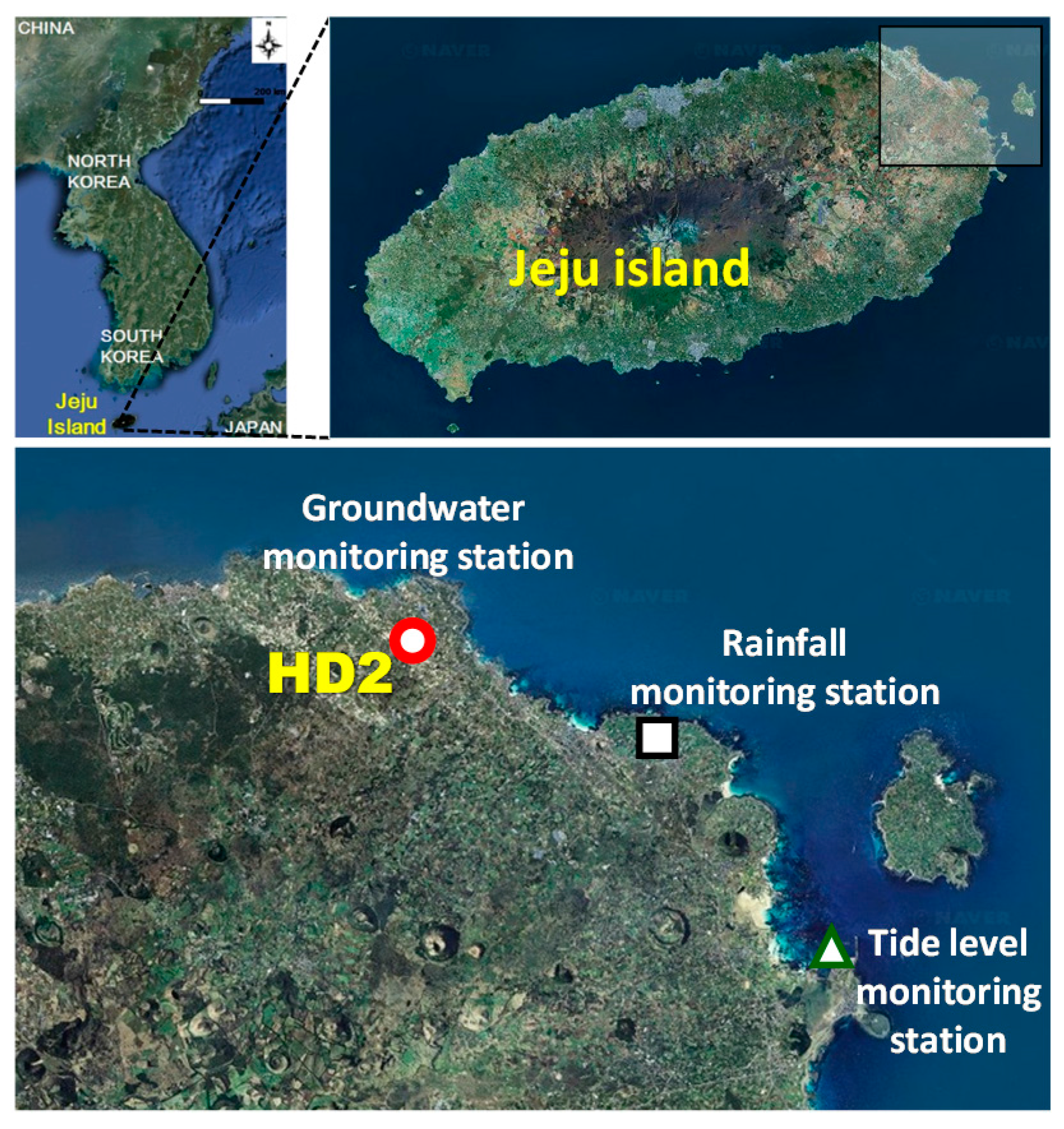
Figure 2.
Vertical profile of electrical conductivity at the HD2 observatory.

Figure 3.
Schematic diagram of the freshwater-saltwater interface level (FSL) monitoring system using the interface egg (modified from Kim et al. [3]).
Figure 3.
Schematic diagram of the freshwater-saltwater interface level (FSL) monitoring system using the interface egg (modified from Kim et al. [3]).
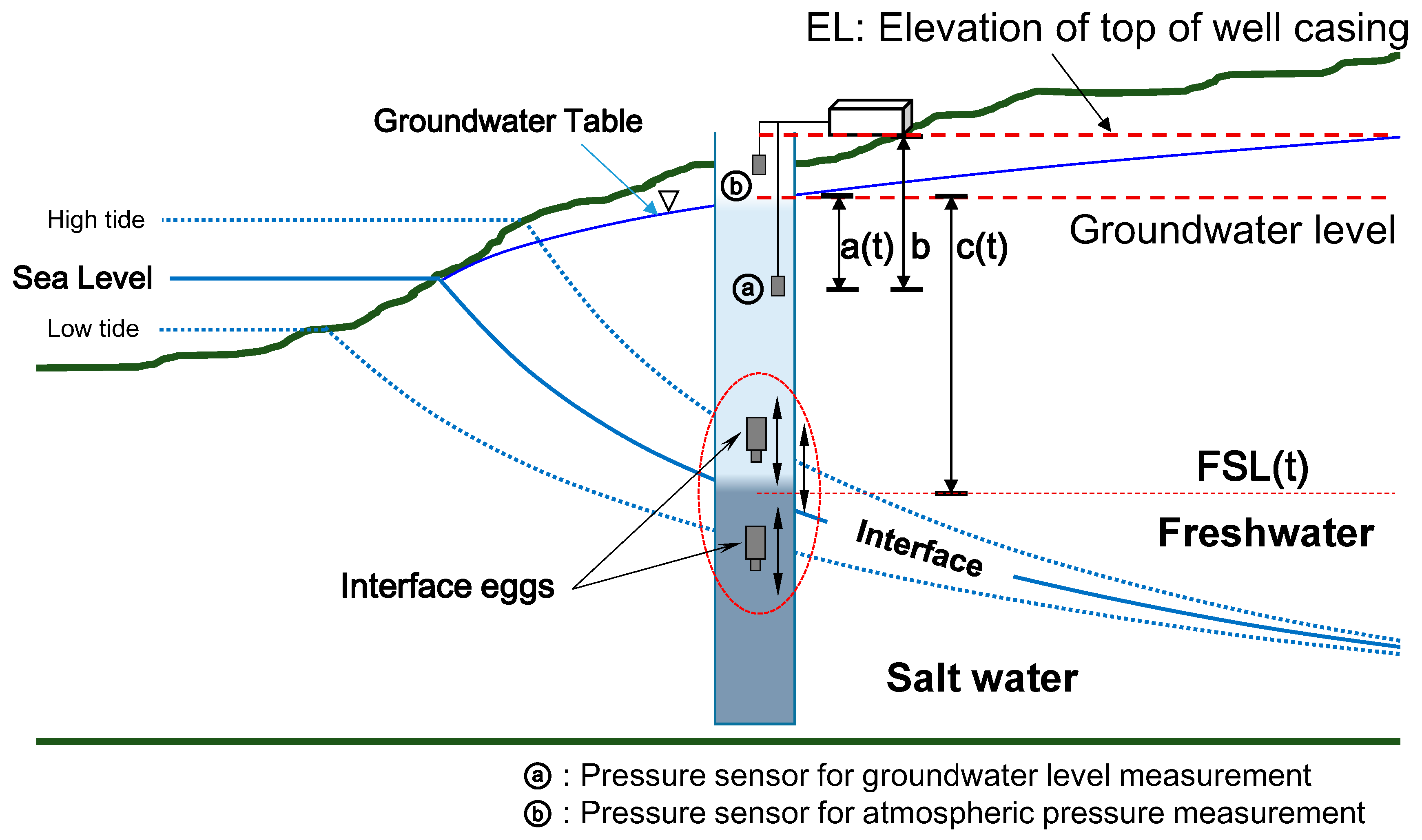
Figure 4.
Time series data of groundwater level (GWL), upper and lower FSL, rainfall and tide level at the HD2 observatory.
Figure 4.
Time series data of groundwater level (GWL), upper and lower FSL, rainfall and tide level at the HD2 observatory.

Figure 5.
Schematic diagrams of the (a) artificial neural network (ANN) and (b) support vector machine (SVM) structure.
Figure 5.
Schematic diagrams of the (a) artificial neural network (ANN) and (b) support vector machine (SVM) structure.
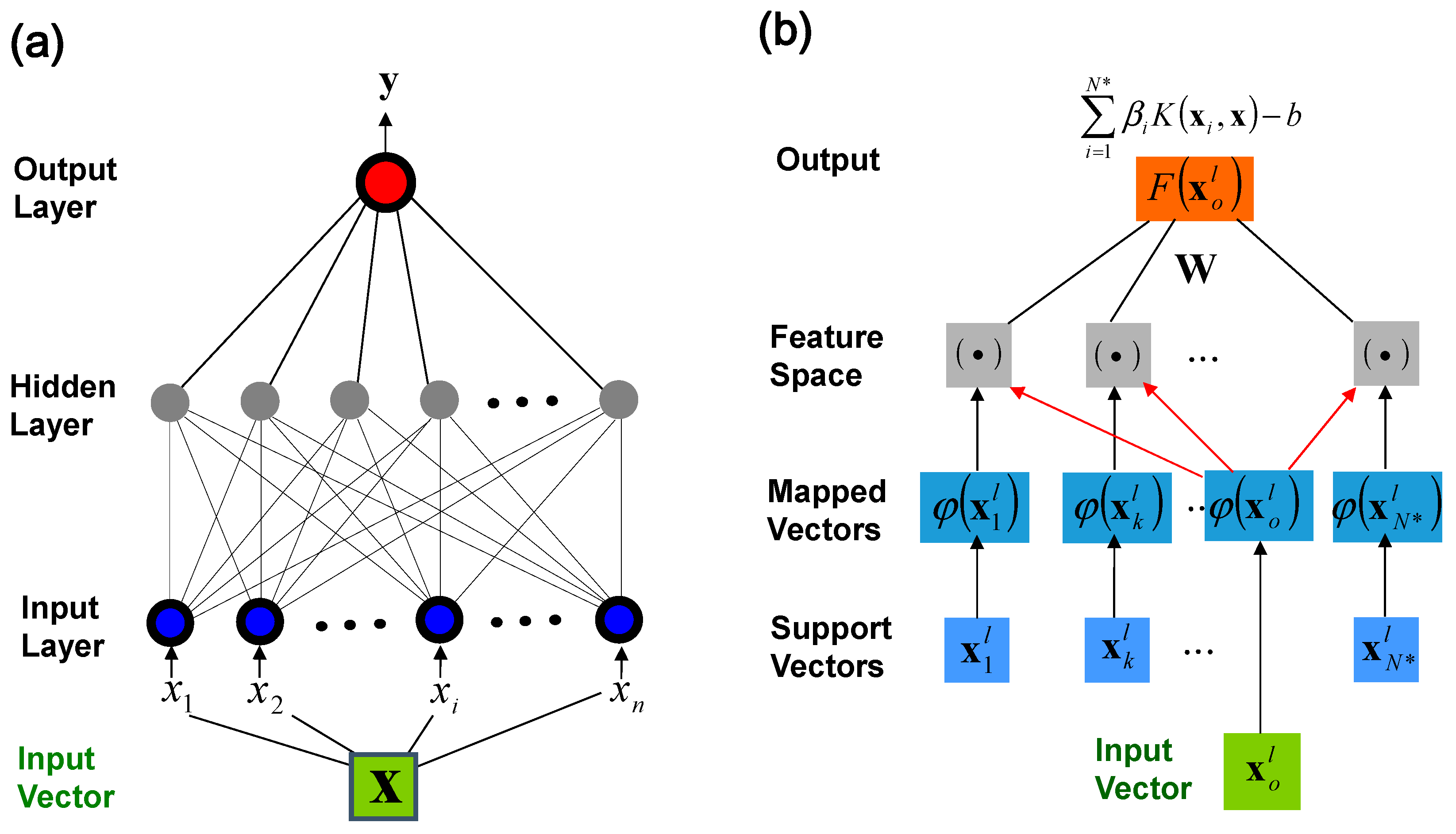
Figure 6.
Direct prediction results for the upper FSL: (a) ANN and (b) SVM.

Figure 7.
Direct prediction results for the lower FSL: (a) ANN and (b) SVM.

Figure 8.
Recursive prediction results for the upper FSL: (a) ANN and (b) SVM.

Figure 9.
Recursive prediction results for the lower FSL: (a) ANN and (b) SVM.
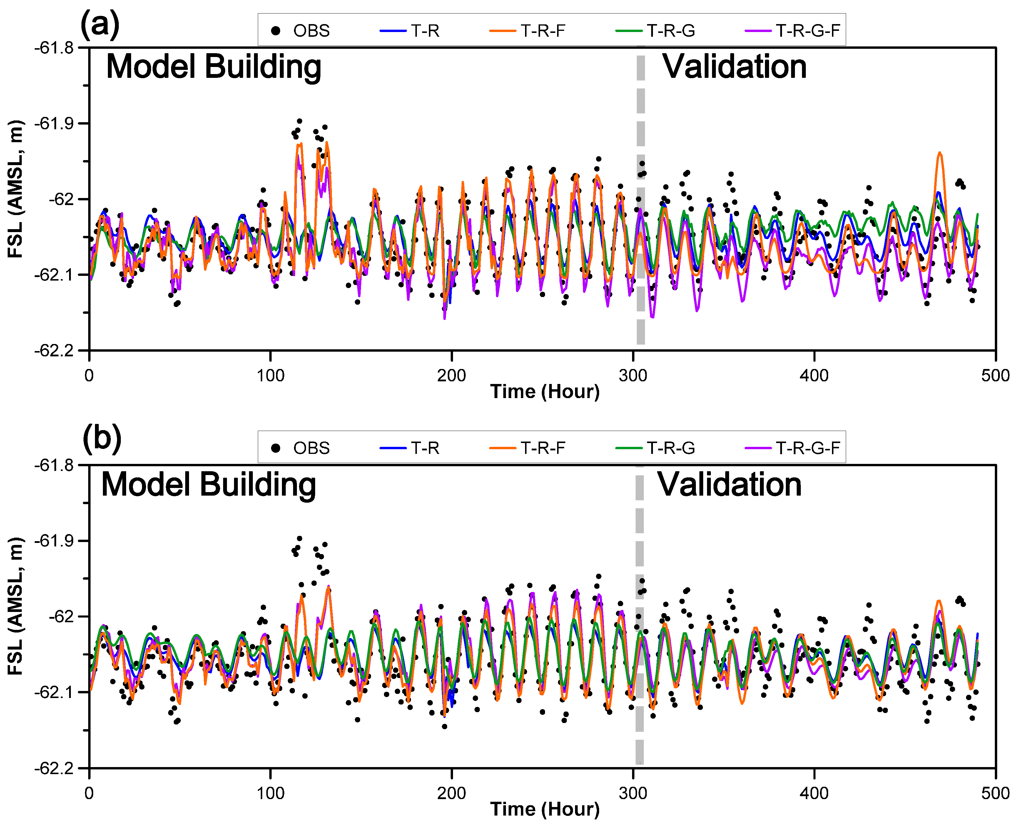
Figure 10.
Comparison of RP-DP ratio values for ANN and SVM models: (a) T-R-F type model for upper FSL; (b) T-R-G-F type model for upper FSL; (c) T-R-F model for lower FSL; (d) T-R-G-F type model for lower FSL.
Figure 10.
Comparison of RP-DP ratio values for ANN and SVM models: (a) T-R-F type model for upper FSL; (b) T-R-G-F type model for upper FSL; (c) T-R-F model for lower FSL; (d) T-R-G-F type model for lower FSL.


Table 1.
Results of cross correlation analysis for measured time series data at the HD2 observatory.
Table 1.
Results of cross correlation analysis for measured time series data at the HD2 observatory.
| Variables | Max. Correlation Coefficient | Lag Time (Hour) |
|---|---|---|
| T-G | 0.85 | 2 |
| R-G | 0.14 | 43 |
| T-F (upper) | 0.83 | 2 |
| R-F (upper) | 0.11 | 47 |
| G-F (upper) | 0.97 | 0 |
| T-F (Lower) | 0.56 | 6 |
| R-F (Lower) | 0.27 | 19 |
| G-F (Lower) | 0.54 | 4 |
Notes: Where T: tide; R: rainfall; G: groundwater level; F: interface level.
Table 2.
Model input structures and the number of components for each variable.
| Input Structures (Model Type) | Number of Components for Variables | |||||
|---|---|---|---|---|---|---|
| T | R | G | F | Total | ||
| Upper FSL | T-R | 4 | 4 | – | – | 8 |
| T-R-F | 4 | 4 | – | 4 | 12 | |
| T-R-G | 4 | 4 | 3 | – | 15 | |
| T-R-G-F | 4 | 4 | 3 | 4 | 19 | |
| Lower FSL | T-R | 8 | 4 | – | – | 12 |
| T-R-F | 8 | 4 | – | 4 | 16 | |
| T-R-G | 8 | 4 | 5 | – | 17 | |
| T-R-G-F | 8 | 4 | 5 | 4 | 21 | |
Notes: Where T: tide; R: rainfall; G: groundwater level; F: interface level.
Table 3.
Data allocation for time series model building and validation.
| Data Type | Data Allocation | ||
|---|---|---|---|
| Model Building | Model Validation | ||
| Upper FSL | Num. data | 250 | 247 |
| Time | 7:00 15 September–12:00 21 September | 13:00 21 September–23:00 5 October | |
| Lower FSL | Num. data | 300 | 197 |
| Time | 7:00 15 September–17:00 27 September | 18:00 27 September–23:00 5 October | |
Table 4.
The selected ANN and SVM model parameters for the FSL prediction.
| Model Type | ANN | SVM | |||||
|---|---|---|---|---|---|---|---|
| HN | LR | MM | C | Eps | Sig | ||
| Upper FSL | T-R | 2 | 0.001 | 0.0 | 7.0 | 0.13 | 3.0 |
| T-R-F | 15 | 0.020 | 0.0 | 5.0 | 0.05 | 2.5 | |
| T-R-G | 2 | 0.005 | 0.3 | 7.0 | 0.10 | 3.0 | |
| T-R-G-F | 5 | 0.005 | 0.0 | 10.0 | 0.05 | 3.0 | |
| Lower FSL | T-R | 15 | 0.001 | 0.9 | 3.0 | 0.11 | 2.0 |
| T-R-F | 15 | 0.001 | 0.3 | 5.0 | 0.13 | 3.0 | |
| T-R-G | 20 | 0.001 | 0.9 | 0.5 | 0.13 | 2.5 | |
| T-R-G-F | 10 | 0.001 | 0.0 | 5.0 | 0.13 | 3.0 | |
Table 5.
Model performance criteria values for the direct prediction of upper FSL.
| Model | Index | T-R | T-R-F | T-R-G | T-R-G-F | Average |
|---|---|---|---|---|---|---|
| ANN | RMSE (m) | 0.061 | 0.034 | 0.042 | 0.032 | 0.042 |
| MARE (%) | 10.329 | 5.901 | 7.083 | 5.613 | 7.232 | |
| CORR | 0.888 | 0.965 | 0.935 | 0.964 | 0.938 | |
| SVM | RMSE (m) | 0.072 | 0.029 | 0.038 | 0.023 | 0.040 |
| MARE (%) | 12.335 | 4.959 | 6.221 | 3.944 | 6.865 | |
| CORR | 0.882 | 0.982 | 0.954 | 0.980 | 0.949 |
Table 6.
Model performance criteria values for the direct prediction of lower FSL.
| Model | Index | T-R | T-R-F | T-R-G | T-R-G-F | Average |
|---|---|---|---|---|---|---|
| ANN | RMSE (m) | 0.034 | 0.020 | 0.040 | 0.020 | 0.028 |
| MARE (%) | 15.314 | 8.438 | 18.494 | 8.623 | 12.717 | |
| CORR | 0.593 | 0.885 | 0.549 | 0.908 | 0.734 | |
| SVM | RMSE (m) | 0.028 | 0.022 | 0.030 | 0.021 | 0.025 |
| MARE (%) | 12.630 | 9.229 | 12.654 | 9.104 | 10.904 | |
| CORR | 0.777 | 0.859 | 0.733 | 0.867 | 0.809 |
Table 7.
Model performance criteria values for the recursive prediction of upper FSL.
| Model | Index | T-R | T-R-F | T-R-G | T-R-G-F | Average |
|---|---|---|---|---|---|---|
| ANN | RMSE (m) | 0.061 | 0.061 | 0.042 | 0.056 | 0.055 |
| MARE (%) | 10.329 | 10.582 | 7.083 | 9.852 | 9.462 | |
| CORR | 0.888 | 0.965 | 0.935 | 0.892 | 0.902 | |
| SVM | RMSE (m) | 0.072 | 0.069 | 0.038 | 0.040 | 0.055 |
| MARE (%) | 12.335 | 12.255 | 6.221 | 7.043 | 9.463 | |
| CORR | 0.882 | 0.920 | 0.954 | 0.943 | 0.925 |
Table 8.
Model performance criteria values for the recursive prediction of lower FSL.
| Model | Index | T-R | T-R-F | T-R-G | T-R-G-F | Average |
|---|---|---|---|---|---|---|
| ANN | RMSE (m) | 0.034 | 0.042 | 0.040 | 0.034 | 0.037 |
| MARE (%) | 15.314 | 16.837 | 18.494 | 14.937 | 16.395 | |
| CORR | 0.593 | 0.420 | 0.549 | 0.806 | 0.592 | |
| SVM | RMSE (m) | 0.028 | 0.034 | 0.030 | 0.035 | 0.032 |
| MARE (%) | 12.630 | 14.347 | 12.654 | 14.773 | 13.601 | |
| CORR | 0.777 | 0.611 | 0.733 | 0.592 | 0.678 |
© 2017 by the authors. Licensee MDPI, Basel, Switzerland. This article is an open access article distributed under the terms and conditions of the Creative Commons Attribution (CC BY) license (http://creativecommons.org/licenses/by/4.0/).
Share and Cite
MDPI and ACS Style
Yoon, H.; Kim, Y.; Ha, K.; Lee, S.-H.; Kim, G.-P. Comparative Evaluation of ANN- and SVM-Time Series Models for Predicting Freshwater-Saltwater Interface Fluctuations. Water 2017, 9, 323. https://doi.org/10.3390/w9050323
AMA Style
Yoon H, Kim Y, Ha K, Lee S-H, Kim G-P. Comparative Evaluation of ANN- and SVM-Time Series Models for Predicting Freshwater-Saltwater Interface Fluctuations. Water. 2017; 9(5):323. https://doi.org/10.3390/w9050323
Chicago/Turabian StyleYoon, Heesung, Yongcheol Kim, Kyoochul Ha, Soo-Hyoung Lee, and Gee-Pyo Kim. 2017. "Comparative Evaluation of ANN- and SVM-Time Series Models for Predicting Freshwater-Saltwater Interface Fluctuations" Water 9, no. 5: 323. https://doi.org/10.3390/w9050323
Note that from the first issue of 2016, this journal uses article numbers instead of page numbers. See further details here.