
Coupled Infiltration and Kinematic-Wave Runoff Simulation in Slopes: Implications for Slope Stability


Department of Geography, University of California, Santa Barbara, CA 93106, USA
*
Author to whom correspondence should be addressed.
Water 2017, 9(5), 327; https://doi.org/10.3390/w9050327
Submission received: 30 March 2017
/
Revised: 29 April 2017
/
Accepted: 2 May 2017
/
Published: 5 May 2017
(This article belongs to the Special Issue Water-Soil-Vegetation Dynamic Interactions in Changing Climate)
Abstract
:Shallow translational slides are common in slopes during heavy rainfall. The classic model for the occurrence of translational slides in long slopes assumes rising saturation above a slip surface that reduces the frictional strength by decreasing the effective stress along soil discontinuities. The classic model for translational slope failure does not conform well to the nature of homogenous soils that do not exhibit discontinuities propitious to create perched groundwater over the soil discontinuity or slip surface. This paper develops an alternative methodology for the coupled numerical simulation of runoff and infiltration caused by variable rainfall falling on a slope. The advancing depth of infiltration is shown to affect the translational stability of long slopes subjected to rainfall, without assuming the perching of soil water over the slip surface. This new model offers an alternative mechanism for the translational stability of slopes that are saturated from the slope surface downwards. A computational example illustrates this paper’s methodology.
1. Introduction
The infiltration of water on slopes is a common cause of slope failure. The source of the water might be rainfall, snowmelt, irrigation, or leaking structures. Rainfall falling on a slope is partitioned into overland flow (runoff, henceforth) and infiltration. The mechanism governing the partition of rainfall water into runoff or infiltration depends on a number of factors: the rainfall intensity and its temporal distribution, the angle of the slope, the infiltration rate at the slope surface, the hydraulic characteristics of the soil underlying the slope, the moisture content distribution through the soil profile, and the hydraulic characteristics of the slope surface. Infiltrated water moves downward through the soil profile and changes the soil’s pore water pressure, its apparent cohesion, and its unit weight. Those changes may affect the stability of the slope to the point of causing sliding. The cause of slope failure is the increased moisture content through the soil profile and its effects on the soil’s unit weight, the soil’s shear strength parameters, and the effective stress on the slip (or failure) surface [1,2,3,4,5,6,7].
There are two classic models of translational slope stability. Both models apply to “infinite” slopes, which practically means that the thickness () of the sliding soil mass is much smaller than the length () of the slope, say, 30, and is commonly less than 2 m [7], although it may be deeper. The first model of the translational stability of long slopes is widely used [5]. It prescribes a phreatic surface parallel to the ground surface and the slip surface, as shown in Figure 1.
, , , , , , and in Figure 1 denote the thickness of the sliding mass, the pore pressure exerted along the slip surface, the thickness zone of saturation above the slip surface, the moist unit weight of the soil, the soil’s saturated unit weight, and the unit weight of the water ( = 9.81 kN/m3), respectively. The stability of the slope decreases as the thickness of saturation increases. The degree of stability is measured by the factor of safety (FS) of the slope soil, which equals the ratio of the forces resisting sliding to the forces driving sliding. A slope with an FS value larger than 1 is stable, it is at limiting equilibrium when FS = 1, and it fails if FS < 1. It is known (see, e.g., [7]) that the FS of the long slope in Figure 1 associated with effective stress analysis is given by the following equation:
in which , , and denote the soil’s cohesion (or cohesive strength), the average unit weight of the sliding mass (), and the angle of friction of the soil, respectively. The reasons for slope failure as the saturated thickness increases are evident. The first term on the right-hand side of Equation (1) is cohesion related. It decreases as increases, thus lowering the FS. This is because the average unit weight of the sliding soil mass increases with increasing . In addition, the expression within the parentheses of the second term on the right hand side of Equation (1) decreases with increasing , is equal to 1 when = 0, and is equal to , or about ½, when . A slope becomes unstable whenever a rising lowers its factor of safety below 1.
The long-slope stability condition depicted in Figure 1 and quantified by Equation (1) does not explain how water enters the soil and moves through it. It implies that water enters the soil and becomes perched above the slip surface, which is found at a depth below the ground surface. For this to happen, there must be a change of soil properties or discontinuity at depth coinciding with the slip surface, where the soil beneath the depth must have a hydraulic conductivity smaller than that of the overlying soil.
Loáiciga et al. [7] provides details of a second model of translational slope stability whereby the phreatic surface emerges from long slopes. This second model also assumes the existence of unconfined, perched, groundwater over a slip surface. Several authors have proposed slope stability models for rotational slides (see, e.g., [8,9]), and three-dimensional stress-strain models of slope deformation and failure solved by finite elements [10]. This paper deals with translational slides occurring on long slopes where the phreatic surface is parallel to the slope and slip surfaces (see Figure 1), and the source of water is rainfall.
The classic model of translational stability represented by Figure 1 and Equation (1) does not take into account the intensity and temporal distribution of rainfall falling on a slope, nor does it consider how much of that rainfall leaves the slope as runoff. It assumes that there is a source of water that saturates the soil over the thickness above the slip surface. This paper develops a methodology for the coupled numerical simulation of runoff and infiltration caused by variable rainfall falling on a slope that accounts for changing soil moisture conditions. The depth of infiltration is shown to affect the translational stability of long slopes subjected to rainfall, without assuming a perching of soil water over the slip surface. This new model offers an alternative mechanism for the translational stability of slopes to that of the classic model represented by Figure 1 and Equation (1).
Iverson [3] proposed a theory for the translational stability of long slopes caused by rainfall relying on a 1-D version of Richards’ infiltration equation in the analysis. A steady-state version of the latter equation was applied to the analysis of long-term slope stability, and a linearized simplification of the 1-D version of the Richards equation was employed to study short-term slope stability. The input of variable rainfall at the slope surface was handled in Iverson’s [3] short-term analysis via a boundary condition of infiltration at the slope surface, and by the superposition of solutions of the linearized simplification of the 1-D version of the Richards equation to account for variable rainfall. Rainfall in excess of the soil’s infiltration capacity (or maximum infiltration rate in Iverson’s terminology) becomes runoff that does not influence the infiltration process [3]. It is relevant at this juncture that Iverson’s simplified infiltration equation for the short-term analysis of translational slope stability implies the piston-flow type displacement of the wetting front that descends from the slope surface, driven by water input at the surface. It has, in this sense, some similarity with Green and Ampt’s [11] infiltration model (see also, [12]), which is applied in the present work. There are several key differences between the present work and Iverson’s [3]. First, this work numerically solves the coupled equations of infiltration and runoff during variable rainfall, which includes the calculation of the depth of overland flow on the slope surface. Secondly, infiltration is driven by a generalized version of the Green and Ampt model, with a variable depth of water on the slope surface. Thirdly, translational slope stability is assessed by calculating the effect that the wetting front has on the factor of safety as it moves downward through the soil profile. Lastly, the numerical model for assessing runoff and infiltration can be simulated for any arbitrary period during which infiltration is driven by rainfall. Slope stability is assessed as a function of the advancing wetting front, the slope geometry, the soil’s unit weight, and shear-strength properties.
2. The Generic Layout of a Slope Subjected to Rainfall that May Undergo Translational Sliding
Figure 2 depicts the various fluxes and geometric variables that are included in this paper’s coupled analysis of rainfall, runoff, infiltration, and slope stability. The following notation is introduced in Figure 1: : station index for the longitudinal coordinate that measures the distance from at the highest point of the sliding mass to at the toe of the sliding mass, where ; denotes the time index, starting with = 0 at the start of rainfall; : the infiltration rate (at the slope surface) at position and time ; : the length of the slope analyzed for slope stability = ; : the overland flow at the toe of the slope per unit width of the slope perpendicular to the plane of Figure 2; : the rainfall rate falling on the slope; : the angle of the slope; : the longitudinal coordinate that coincides with the slope surface; : the depth of runoff measured vertically between the slope surface and the water surface as shown in Figure 2; : the depth of the wetting front at position and time : the discretization interval, or length step, for the longitudinal coordinate .
3. Kinematic-Wave Runoff Affected by Rainfall and Infiltration
Runoff on a slope surface is wide and shallow, so that the hydraulic radius is approximately equal to . Runoff is herein modeled with the kinematic-wave approximation to the equation of 1-D (shallow and wide) overland flow, with accretion by rainfall and depletion by infiltration (see, e.g., [13,14,15]):
In Equation (2), is the depth of runoff, and denote the infiltration rate and rainfall rate, respectively, and the derivative of the infiltration with respect to time is represented by = . The coefficients = 5/3, ; is defined by the following equation:
where and denote the Manning’s roughness coefficient and the slope of the terrain, respectively. The initial condition of Equation (2) is as follows:
in which denotes the time at which runoff emerges on the slope. The boundary condition of Equation (2) at the upstream end is as follows:
The overland flow (in m3/s per unit width of slope) at location and time is given by Manning’s equation:
The next sections present the infiltration model developed in this work.
4. Infiltration on a Slope
Infiltration is herein modeled with the 1-D Green and Ampt model as modified by Loáiciga and Huang [12] for level ground, and further extended in this study for the case of sloping terrain.
4.1. The Elapsed Time of Rainfall Required to Initiate Runoff on a Slope
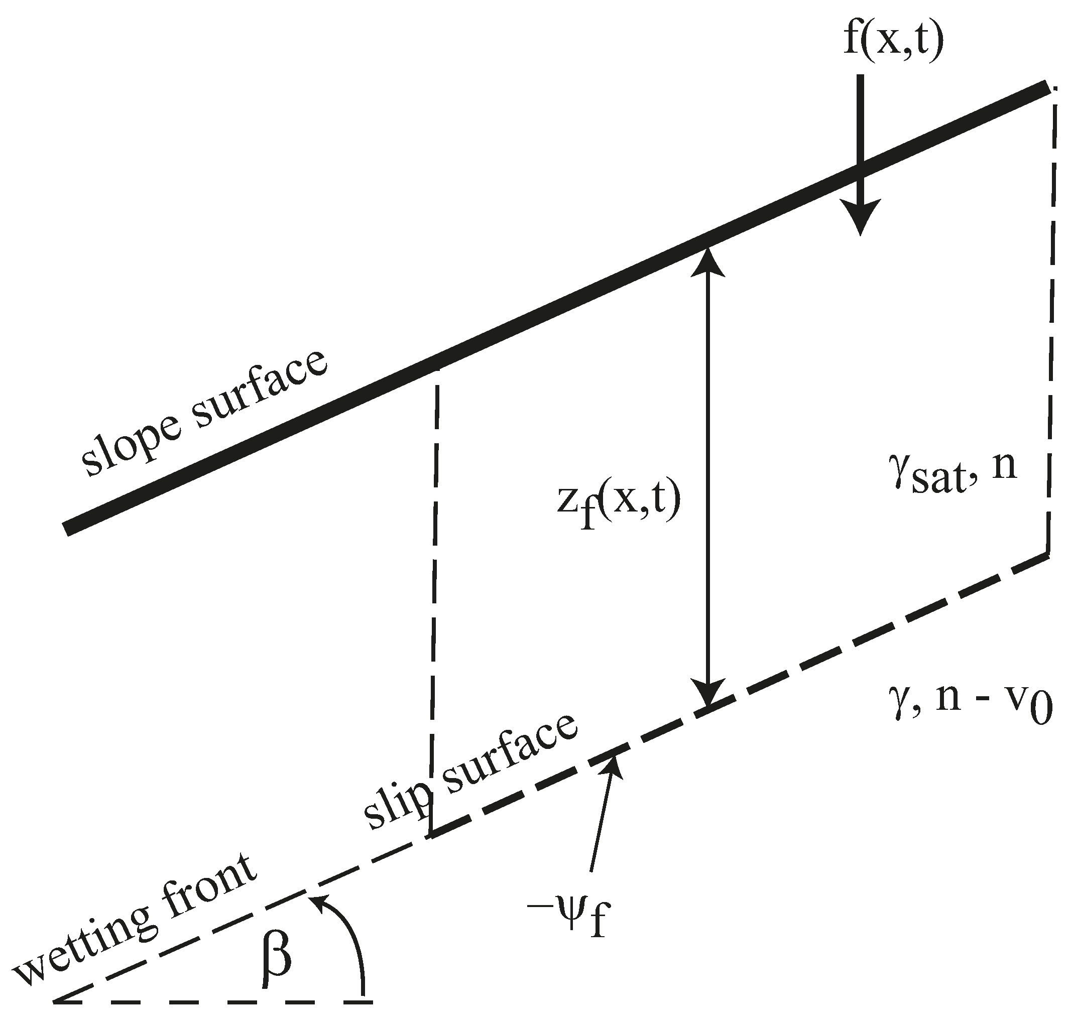
The time required to initiate runoff on a slope depends on the intensity of the rainfall and the saturated hydraulic conductivity () of the slope’s soil. This paper considers the case of variable rainfall . Figure 3 shows a schematic of the infiltration process following Green and Ampt’s model of “piston-flow” displacement of the wetting front.
All of the nomenclature shown in Figure 3 was described above, except for the wetting-front soil-water tension , a soil property, estimable from the textural parameters [16,17,18]. The pressure head on the wetting front equals . The infiltration at position and time , , is given by the following expression under the assumption of a uniform distribution of the volumetric water content () on the slope’s soil:
in which represents the soil’s porosity. The Darcian flux at the slope’s surface is the infiltration rate, which equals the rainfall rate prior to the formation of runoff. In this case, Darcy’s law written between the slope surface and the wetting front yields:
in which denotes the soil’s saturated hydraulic conductivity.
denotes the cumulative rainfall, which equals the time integral of the left-hand side of Equation (8), or:
The cumulative rainfall equals the infiltration prior to runoff formation. Therefore:
prior to runoff formation. Runoff begins at time when the cumulative rainfall exceeds infiltration. The time is found by solving the integral form of Equation (8):
The solution of Equation (11) is the time to the initiation of runoff, , that makes the left-hand side equal to the right-hand side. The rainfall hyetograph is herein expressed as a sequence of rainfall rates falling on a station of the slope, , ; , whereby each rainfall rate has a duration equal to the time step . This time step is equal to the numerical simulation step employed in the solution of the coupled runoff and infiltration equations. Therefore, the discrete form of Equation (11) applied to determine the time at which runoff begins, is as follows:
where is such that . The time is easily calculated graphically. The application of Equation (12) is illustrated in this work’s computational example. The time is obtained by solving the following equation in the case of constant rainfall :
which is only solvable if . Otherwise, runoff does not form on the slope surface. The time to ponding makes the left-hand side of Equation (13) equal to its right-hand side.
4.2. Infiltration after Runoff Formation
The second phase of infiltration occurs in the period when there is runoff on the slope and there is rainfall falling. The pressure head at the slope surface is approximately equal to (see Figure 2):
Darcy’s law written between the slope surface and the wetting front yields:
The substitution of Equation (7) into Equation (15) and subsequent algebraic rearrangement produces the following partial differential equation:
where:
The initial condition associated with Equation (16) is:
in which denotes the infiltration at time :
The upstream boundary condition associated with Equation (16) considers that the depth of runoff at = 0 equals , and, thus, Equation (15) reduces to the following boundary condition:
It is noteworthy that after solving the infiltration , the depth to the wetting front () is calculable from Equation (7). Equations (2) and (16) constitute two coupled, nonlinear, partial differential equations. Their solution is discussed in Section 5. The simulation of Equations (2) and (16) is herein carried out until the time when a rainfall event ends. Thereafter, the depth of runoff quickly vanishes on the slope and the wetting front ceases to advance downward under the assumptions of the Green and Ampt model. The analysis of slope stability is applied considering the downward advance of the wetting front driven by rainfall, as described in Section 6.
Several approaches have been reported that calculate a rainfall excess in each rainfall interval , whereby the rainfall excess equals the excess of rainfall falling in the interval over the incremental infiltration occurring in the same interval (see a review in Dingman [18]). Those approaches, however, do not simulate the joint dynamical equations of runoff and infiltration in the sloping terrain and the effect that infiltration has on the translational stability of long slopes.
5. Numerical Solution of the Coupled Infiltration and Runoff Equations
5.1. Finite-Difference Discretization of the Runoff Equation
This study presents an explicit numerical scheme to jointly solve the runoff Equation (2) and the infiltration Equation (16). The explicit scheme requires that the simulation time step meet the following stability condition for the kinematic wave modeling of runoff [19]:
in which = 981 cm/s is the acceleration of gravity and denotes the depth of runoff (shown in Figure 2). The spatial step must be chosen to provide an adequate resolution along the length of the slope. For illustration, suppose that the spatial step is equal to 100 cm and the depth of runoff equals 10 cm. Therefore, Equation (22) indicates a time step equal to 1 second for these values. Generally, the explicit scheme involves the simulation of a large number of time steps to solve the coupled runoff and infiltration equations. This, however, does not constitute a computational burden given the current computational speed of personal computers (our model runs in 2 s in a standard laptop computer). Moreover, the explicit solution scheme avoids the complexity of solving a system of coupled nonlinear equations that arises when one chooses an alternative implicit solution scheme. The explicit finite-difference discretization of the runoff Equation (2) is as follows:
, and , in which:
The initial time corresponds to the time of the initiation of runoff, . Notice that Equation (23) involves the unknown depth of runoff and the unknown infiltration . These variables’ values are known at the previous time step . The initial condition associated with Equation (23) is:
The upstream boundary condition associated with Equation (23) is given by:
The runoff rate is given by the following expression (in (m3/s)/m) :
5.2. Finite-Difference Discretization of the Infiltration Equation
The finite-difference, explicit, numerical discretization of the infiltration Equation (16) is as follows:
, and , in which:
All other terms appearing in Equation (33) have been previously defined.
The initial condition associated with Equation (33) is:
The boundary condition of Equation (33) is given by the discretized form of Equation (21):
The approach for the joint solution of Equations (23) and (33) is described next.
5.3. Explicit Solution Approach to the Runoff and Infiltration Equations
The finite-difference Equation (23) for runoff is rewritten in a simplified form, as follows:
, and , (recall that = 0) in which:
All other terms appearing in Equation (37) were defined previously. The discretized infiltration Equation (33) is rewritten as follows:
, and , in which:
Equation (40) for is substituted into Equation (37) to yield an explicit equation for the runoff depth in the -th computational period:
, and , (recall that = 0) in which:
Equation (44) represents the explicit formulation for calculating the runoff depth. For physical stability, must be equal to or larger than zero. Once , is calculated, its value is employed in Equation (40) to calculate , . Recall that is given by the boundary condition (36). At this juncture, the computational time is increased to to calculate , followed by the calculation of . The iterative calculations end when the runoff depth becomes equal to zero on the slope. The depth to the wetting front at any computational location and time is calculated as follows:
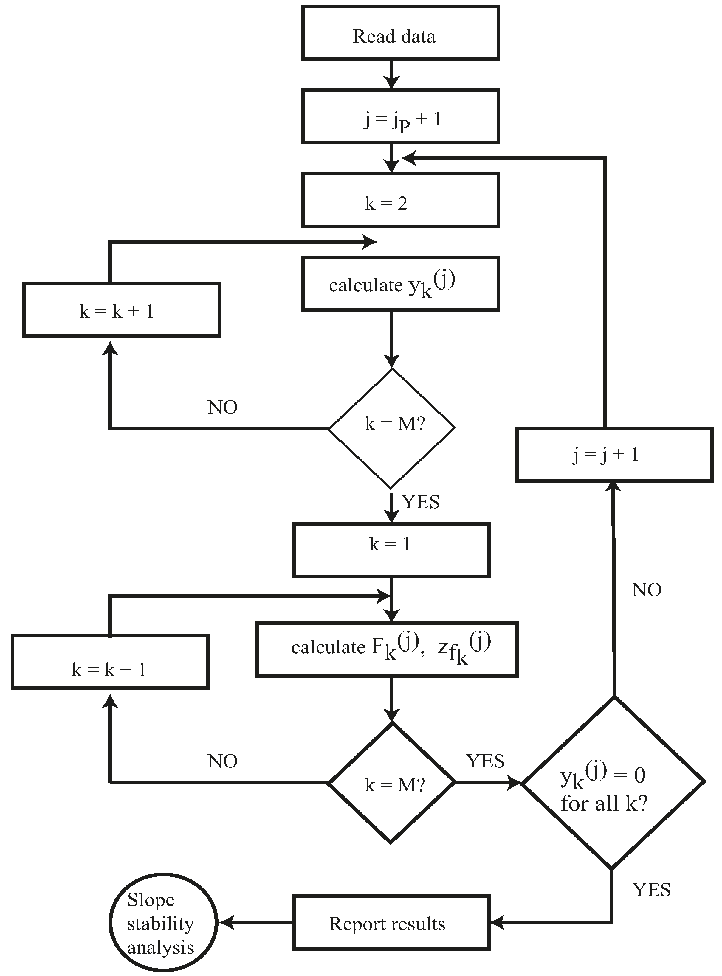
in which ; Figure 4 depicts the flowchart of the algorithm used for the numerical solution of the runoff and infiltration equations on a slope.
6. Translational Stability Analysis of Long Slopes
This paper fundamentally departs from the classic long-slope, translational, failure mechanism embodied by Equation (1) and diagramed in Figure 1. Figure 5 depicts an advancing wetting front on the sloping terrain. The antecedent soil-moisture deficit equals , with and denoting the porosity and initial volumetric content of the slope soil, respectively. Prior to slope saturation, the soil’s (wet) unit weight equals . The soil within the saturated thickness extending from the surface to the wetting-front depth has a saturated unit weight .
Soil saturation occurs from the slope surface downwards. At some time, the effect of soil saturation by infiltrating rainfall reaches a slip surface along which soil mass slides. The classic translational sliding mechanism, on the other hand, assumes that slope failure is caused by rising saturation above the slip surface. The translational mechanism herein proposed is as follows. Prior to infiltration (i.e., with antecedent conditions prevailing), the factor of safety in the slope’s soil at an arbitrary depth below the ground surface is given by the following expression ( denotes the factor of safety under antecedent conditions derived with effective-stress analysis):
in which denotes the apparent cohesion in the soil created by soil water suction (negative pore pressure under unsaturated conditions).
The apparent cohesion stems exclusively from negative pore pressure and differs from the actual cohesion in cemented soils or in overconsolidated fine-grained soils [5,20]. Soils in which the slope angle exceeds the soil’s angle of friction may be stable due to apparent cohesion.
The soil pressure head developed by a downward-advancing wetting front equals at the wetting front (see Figure 5). The pressure head is larger (that is, less negative) than the pressure head that prevails under antecedent conditions. Therefore, the apparent cohesion is reduced by infiltration to a value of . This follows from a physical consideration of a soil’s characteristic curve relating pore pressure to its volumetric water content: as the volumetric water content increases, the pore pressure becomes less negative (increases), thus reducing the apparent cohesion. The reduced apparent cohesion could be nil in clean, coarse, granular soils. This reduces or nullifies the first term on the right-hand side of Equation (47). There is a second effect that reduces the cohesion-related term on the right-hand side of Equation (47). This stems from the increased unit weight of the soil as it transitions from wet (or even dry conditions) to saturated conditions. The unit weight increases from to . The factor of safety on the wetting front after infiltration () becomes:
The factor of safety in Equation (48) may fall below a value of 1 in soils with a slope angle larger than the angle of friction . A failure condition at the wetting front is assured in this instance if the apparent cohesion vanishes altogether by infiltration, in which case the factor is reduced to the following minimum:
Equation (48) indicates that slope soils whose shear strength relies exclusively on apparent cohesion are particularly vulnerable to translational sliding as the wetting front advances downward. This vulnerability is heightened if dynamic forces are applied during slope wetting [7]. The following section presents the computational results for this paper’s methodology.
7. Results and Discussion
7.1. Data Input for Runoff Simulation
Table 1 lists the hydraulic characteristics of the slope chosen for the numerical example.
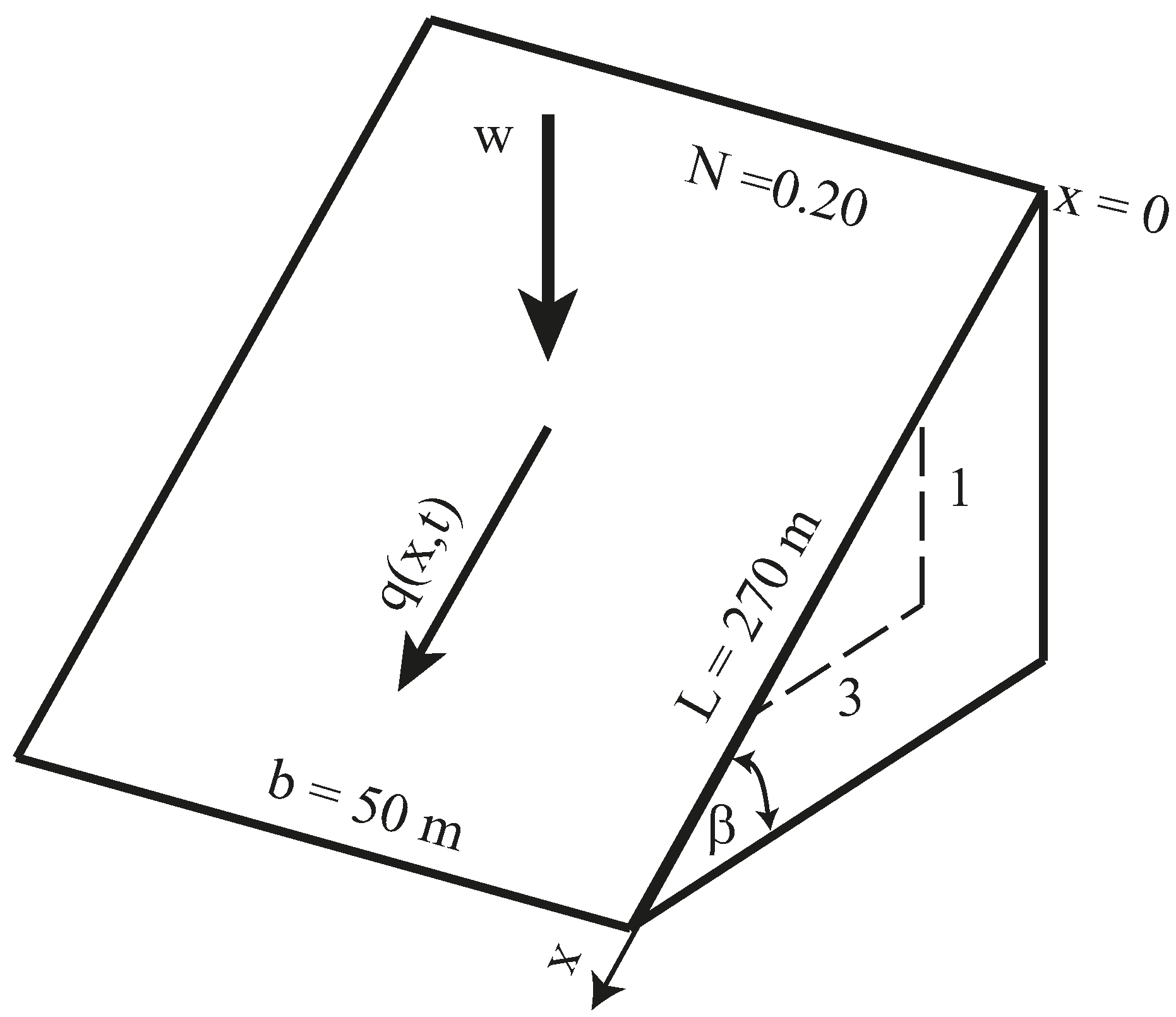
Figure 6 depicts the geometry of the slope controlling the runoff characteristics.
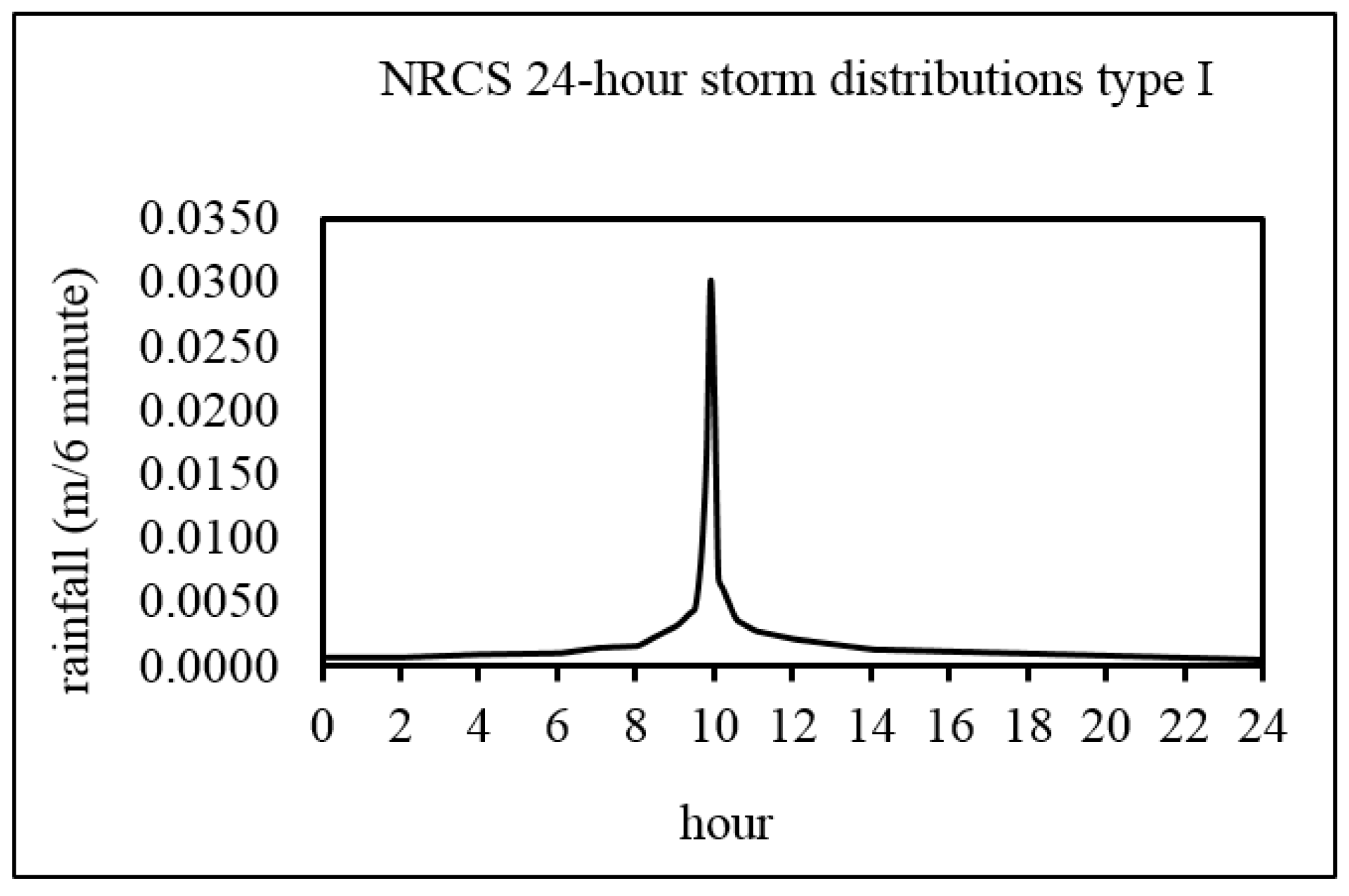
The rainfall input applied in this example follows a United States Department of Agriculture’s (USDA) National Resources Conservation Service (NRCS) type I distribution over a 24-h duration. The total depth of rainfall over its 24-h duration equals 0.40 m in this example. Figure 7 depicts the hyetograph of the rainfall event applied in this example. The maximum rainfall occurs at time 9.9 h with a depth of rainfall equal to 0.030 m falling over a 6-min interval, which is the time interval employed to construct the graph of Figure 7.
The computational length step was chosen to be equal to 10 m, for = = 30 steps. The computational time step was made equal to 10 s for the numerical stability of the runoff computations (see Equation (22)). A shorter length step would produce a more refined spatial resolution. It would require, however, a shorter time step. For example, a = 1 m would require a 1 second. The shortest temporal resolution for rainfall available was = 10 s, which is consistent with the choice of = 10 m.
7.2. Data Input for Simulation of Infiltration
Table 2 lists the soil characteristics employed in this paper’s computational example.
7.3. The Elapsed Time () of Rainfall Required to Initiate Runoff on the Slope
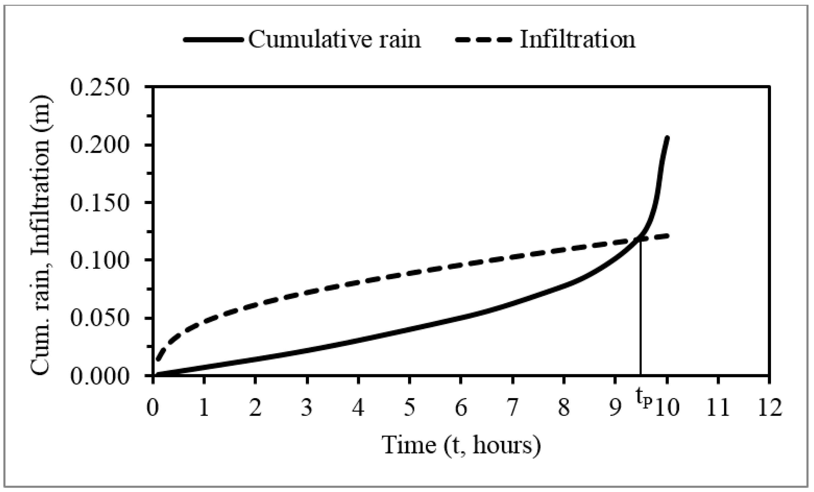
Figure 8 shows the graphical determination of the time , found by graphically solving Equation (12). This is accomplished by finding the time when the left-hand side of Equation (12), which represents cumulative rainfall, equals the right-hand side of Equation (12), which represents the infiltration, as shown in Figure 8. The time at which ponding begins equals 9.5 h = 34,200 s. Notice that only occurs 0.4 h before the time of occurrence of the maximum depth of rainfall, which occurs at 9.9 h (see Figure 7).
The cumulative rainfall equals the infiltration at the initiation of runoff, = 0.118 m, which constitutes the initial condition for the numerical simulation of infiltration. The corresponding depth of infiltration = 0.118/0.20 = 0.590 m.
7.4. Calculated Depth of Runoff and Depth of Infiltration
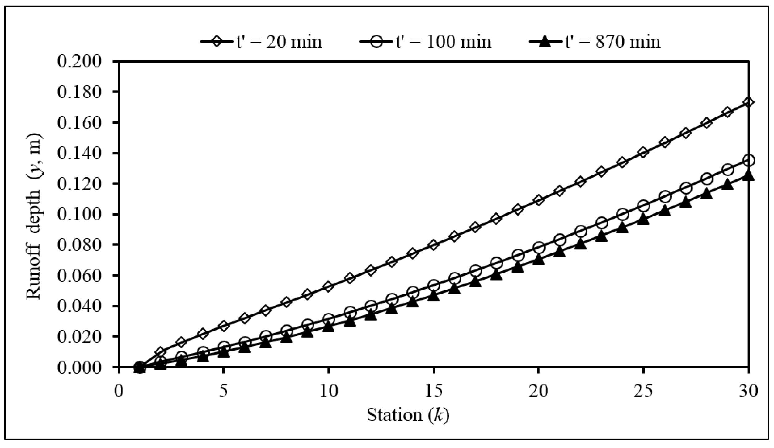
The calculated runoff depth () is shown in Figure 9 for times = 20 (or 1/3), 100 (or 5/3), and 870 (or 14.5) min (h) after ponding began. The latter time coincides with the end of rainfall (24 h after the beginning of rainfall).
As seen in Figure 9, the runoff depth rises with an increasing distance downstream from the slope crown (where = 0 and 0 m). The time elapsed since the beginning of runoff is denoted by , in which = 34,200 s = 570 min = 9.50 h. The runoff depth at = 20 min occurs during the steep rising limb of the hyetograph shown in Figure 8. The runoff depth continues to increase until = 24 min, when the rainfall reaches its maximum intensity (see Figure 7). Thereafter, the runoff decreases, as depicted by the graphs of the runoff depth associated with = 100 min and 870 min. The latter time coincides with the end of rainfall, which lasts 24 h. Thereafter, the runoff depth decreases rapidly to zero everywhere on the slope. The post-rainfall runoff depth is not shown in Figure 9.
Figure 10 depicts the calculated depth of infiltration () for times = 20 (or 1/3), 100 (or 5/3), and 870 (or 14.5) min (h) after ponding began.
Figure 10 shows that the depth of infiltration increases continuously over time. The depth of infiltration increases between stations 1 and 2, the former being the station where the boundary condition is specified. The relatively low infiltration at station 1 is due to the runoff-depth boundary condition 0. Thereafter, it is seen in Figure 10 that the depth of infiltration is nearly uniform over the remainder of the slope. The results depicted in Figure 10 establish that slope stability must be examined between depths of penetration ranging from a few centimeters to about 1.0 m beneath the slope surface for the considered rainfall event. The depth of infiltration increases negligibly after rainfall cessation because the depth of runoff vanishes rapidly without a supply of rain.
7.5. Slope Stability Analysis
The calculations for slope stability analysis presented in this section involve Equation (47) for the factor of safety under antecedent conditions (prior to rainfall, ) and Equation (48) for the factor of safety modified by infiltration (. Table 3 lists the properties employed in the stability analysis. The friction angle herein used is relatively low, typical of landslide debris. The antecedent and infiltration-modified apparent cohesions correspond to 1 m and 0.05 m of soil water tension, respectively, converted to pressure units.
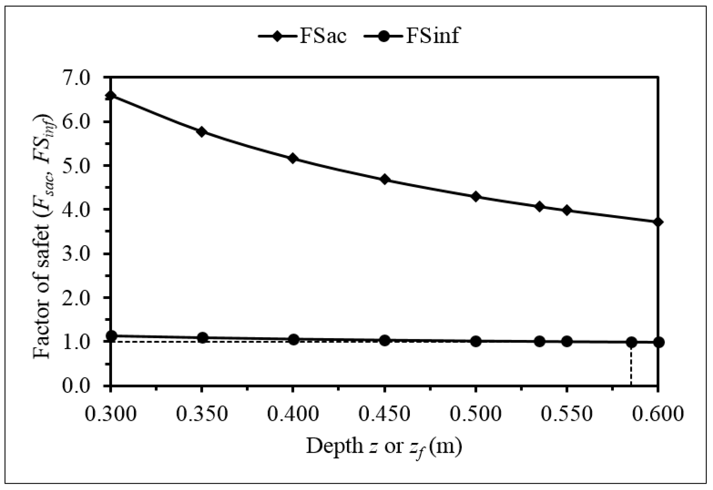
Figure 11 depicts the calculated factors of safety corresponding to antecedent conditions and to conditions modified by infiltration. It is seen in Figure 11 that the slope with antecedent conditions (before rainfall) is stable for various depths beneath the slope surface. The infiltration-modified slope, however, exhibits a slip surface at a depth of the wetting front equal to 0.585 m, where the factor of safety against translational sliding falls below 1. This slip surface is shallower than the depth of infiltration at the initiation of runoff on the slope, which was established above to equal 0.590 m. This means that the critical period for stability under the conditions of this example occurs when all the rainfall infiltrates, prior to ponding. In this example, the rainfall characteristics and soil properties determine the onset of slope failure before the beginning of runoff. Yet, slope failure could occur after the initiation of runoff under other conditions. Notice in Figure 11 that the factor of safety decreases with an increasing depth of the wetting front as a result of the larger body of mass that must be supported by apparent cohesion and friction resistance. The factor of safely is slightly larger than 1 in the range of depth shown in Figure 11, which means that the reduction of the apparent cohesion caused by the advance of the wetting front produces near limit-equilibrium slope stability across the soil profile.
In summary, this paper presented a new methodology for the analysis of the translational stability of long slopes. The methodology jointly simulates the runoff and infiltration on a slope caused by variable rainfall. Infiltration conforms to an extended formulation of the Green and Ampt infiltration model. The slope stability analysis of this paper’s methodology takes into account the effect of the reduction of the apparent cohesion caused by infiltration, and the increase in the soil’s unit weight caused by a downward-moving wetting front. A computational example illustrated the application of this paper’s methodology.
Author Contributions
J. Michael Johnson wrote the MATLAB code to solve the numerical runoff and infiltration equations. Hugo A. Loáiciga developed the Equations (1)–(49).
Conflicts of Interest
The authors declare no conflict of interest.
References
- Cedegreen, H.R. Seepage, Drainage, and Flow Nets; John Wiley & Sons: New York, NY, USA, 1989. [Google Scholar]
- Anderson, S.A.; Sitar, N. Analysis of rainfall-induced debris flows. J. Geotech. Eng. 1995, 121, 544–552. [Google Scholar] [CrossRef]
- Iverson, R.M. Landslide triggering by rain infiltration. Water Resour. Res. 2000, 36, 1897–1910. [Google Scholar] [CrossRef]
- Wang, G.; Sassa, K. Factors affecting rainfall-induced flowslides in laboratory flumes tests. Géotechnique 2001, 51, 587–599. [Google Scholar] [CrossRef]
- Duncan, J.M.; Wright, S.G.; Brandon, T.L. Soil Strength and Slope Stability; John Wiley & Sons: Hoboken, NJ, USA, 2014. [Google Scholar]
- Loáiciga, H.A. Steady-state phreatic surfaces in sloping aquifers. Water Resour. Res. 2005, 41. [Google Scholar] [CrossRef]
- Loáiciga, H.A. Groundwater and Earthquakes: Screening Analyses for Slope Stability. Eng. Geol. 2015, 193, 276–287. [Google Scholar] [CrossRef]
- Morgenstern, N.R.; Price, V.E. The analysis of the stability of general slip surfaces. Géotechnique 1965, 15, 79–93. [Google Scholar] [CrossRef]
- Spencer, E. A method of analysis of the stability of embankments assuming parallel inter-slice forces. Géotechnique 1967, 17, 11–26. [Google Scholar] [CrossRef]
- Griffiths, D.V.; Marquez, R.M. Three-dimensional slope stability by elasto-plastic finite elements. Géotechnique 2007, 57, 537–546. [Google Scholar] [CrossRef]
- Green, W.H.; Ampt, G.A. Studies on soil physics, part I: The flow of air and water through soils. J. Agric. Sci. 1911, 4, 1–24. [Google Scholar]
- Loáiciga, H.A.; Huang, A. Ponding analysis with Green-and-Ampt infiltration. J. Hydrol. Eng. 2007, 12, 109–112. [Google Scholar] [CrossRef]
- Chow, V.T. Open-Channel Flow; McGraw-Hill Kogakusha Ltd.: Tokyo, Japan, 1959. [Google Scholar]
- Cunge, J.A.; Holly, F.M., Jr.; Verwey, A. Practical Aspects of Computational River Hydraulics; Pitman Publishing Ltd.: London, UK, 1980. [Google Scholar]
- Chaudry, H.C. Open-Channel Hydraulics; Prentice Hall: Upper Saddle River, NJ, USA, 1993. [Google Scholar]
- Rawls, W.J.; Brakensiek, D.L. A procedure to predict Green and Ampt infiltration parameters. In Advances in Infiltration; America Society of Agricultural Engineering: St. Joseph, MI, USA, 1983; pp. 102–112. [Google Scholar]
- Rawls, W.J.; Ahuja, L.R.; Bakensiek, D.L.; Shirmohammadi, A. Chapter 5: Infiltration and soil water movement. In Handbook of Hydrology; Maidment, D.R., Ed.; McGraw-Hill: New York, NY, USA, 1992. [Google Scholar]
- Dingman, S.L. Physical Hydrology; Waveland Press: Long Grove, IL, USA, 2015. [Google Scholar]
- Hydrologic Engineering Center. Hydrologic Modeling System HEC-HMS: Technical Reference Manual; United States Corps of Engineers: Davis, CA, USA, 2000. [Google Scholar]
- Holtz, R.D.; Kovacs, W.D.; Sheahan, T.C. An Introduction to Geotechnical Engineering; Pearson Education Inc.: Upper Saddle River, NJ, USA, 2011. [Google Scholar]
Figure 1.
Long slope (elevation view) showing some elements of a translational slide. Not drawn to scale.
Figure 1.
Long slope (elevation view) showing some elements of a translational slide. Not drawn to scale.
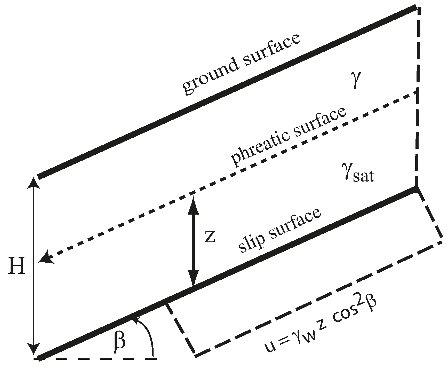
Figure 2.
Generic elevation view of a slope subjected to rainfall and infiltration susceptible to translational sliding. Not drawn to scale.
Figure 2.
Generic elevation view of a slope subjected to rainfall and infiltration susceptible to translational sliding. Not drawn to scale.
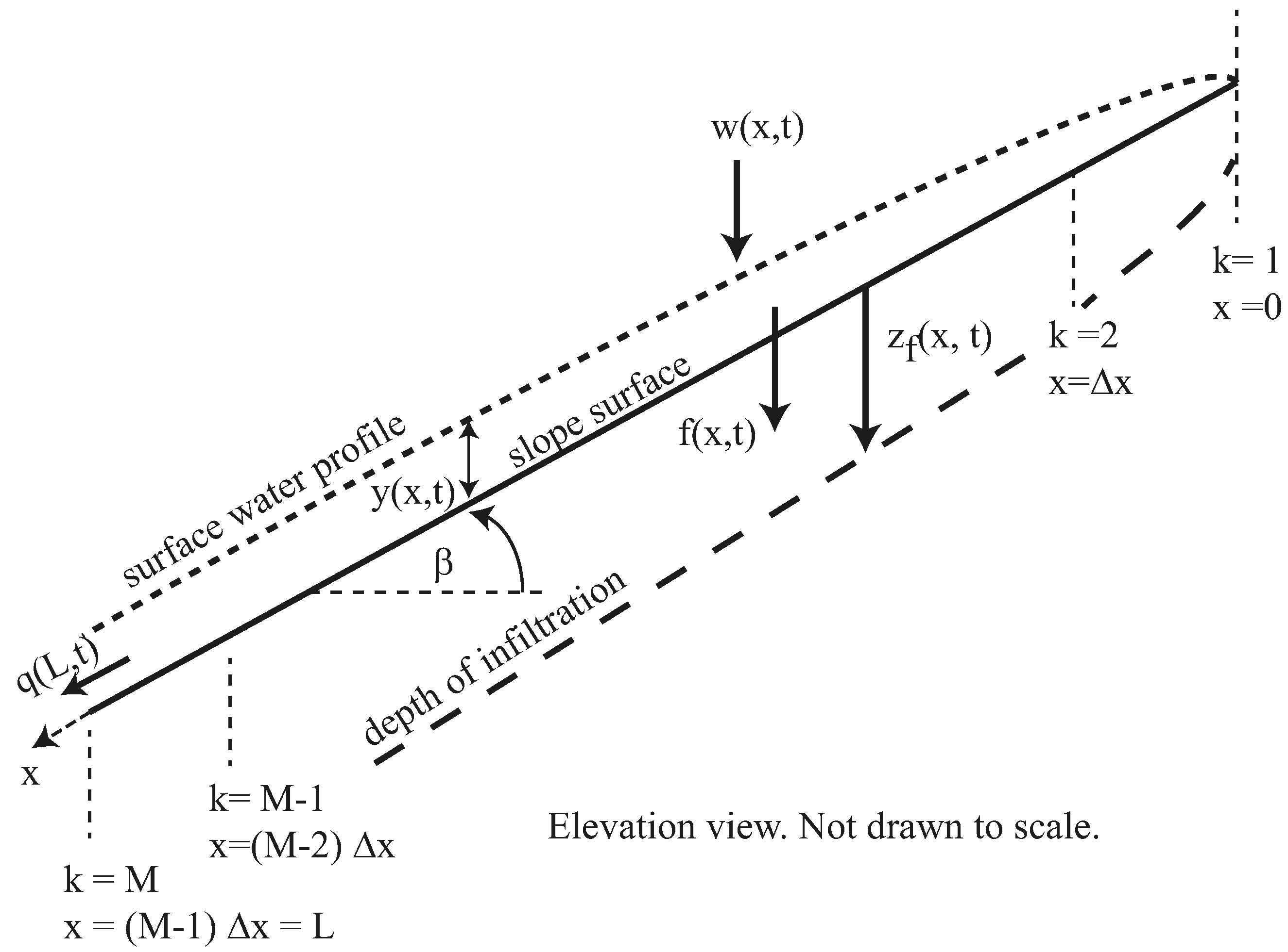
Figure 3.
Schematic of the infiltration process. The pressure head at point is approximately equal to . Elevation view not drawn to scale.
Figure 3.
Schematic of the infiltration process. The pressure head at point is approximately equal to . Elevation view not drawn to scale.
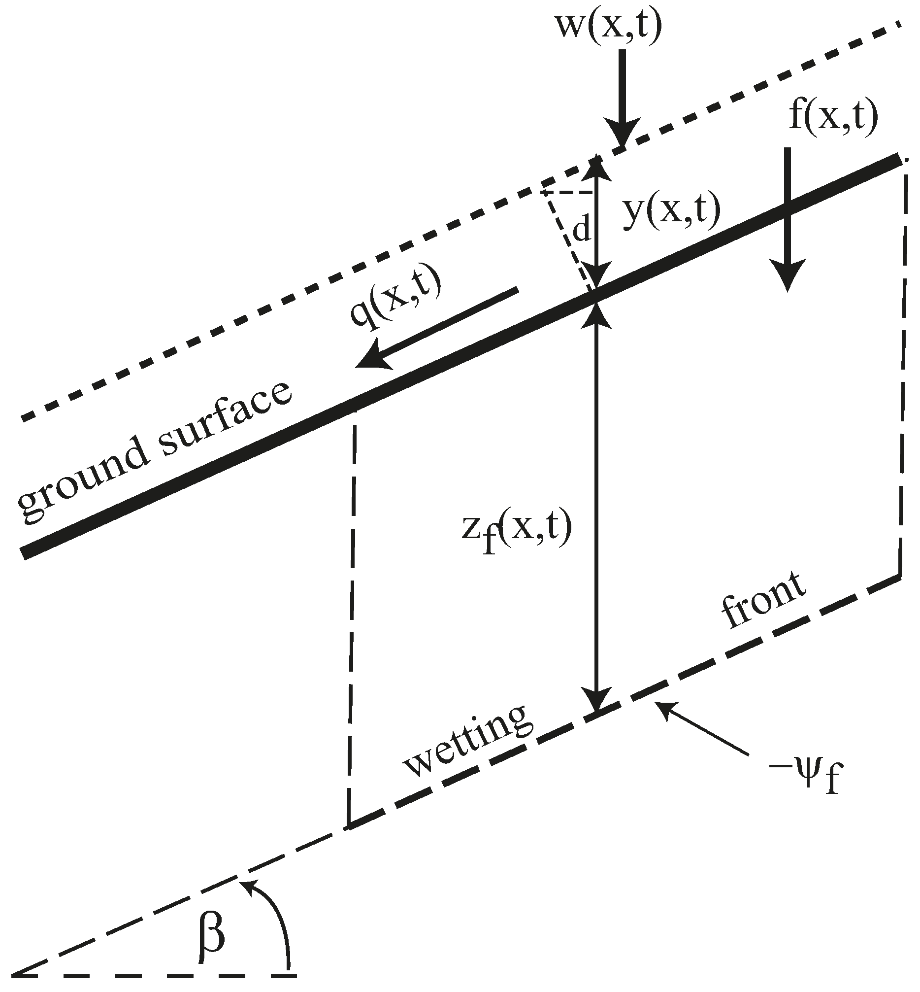
Figure 4.
Algorithmic flowchart for solving the coupled runoff and infiltration equations.

Figure 5.
Diagram of a landslide caused by an advancing wetting front. Elevation view not drawn to scale.
Figure 5.
Diagram of a landslide caused by an advancing wetting front. Elevation view not drawn to scale.

Figure 6.
Geometry and hydraulic characteristics of the runoff example. Not drawn to scale.

Figure 7.
Input 24-h NRCS type I rainfall () event with a total depth equal to 0.40 m.

Figure 8.
Graphical determination of the time = 34,200 s = 9.50 h.

Figure 9.
Calculated runoff depth () as a function of slope station ( ) and time .

Figure 10.
Calculated infiltration depth () as a function of slope station ( ) and time .

Figure 11.
Factors of safety as a function of depth for two moisture regimes.

Table 1.
Runoff data.
| Slope () | Roughness Csdoeff. () | Length (, m) | Width (, m) | Rainfall (, m s−1) |
|---|---|---|---|---|
| 1/3 ( | 0.20 | 270 | 50 | Variable with time (see Figure 7) |
Table 2.
Soil properties.
| Porosity () | Volumetric Water Content () | Wetting-Front Water Tension (, m) | Hydraulic Conductivity (, m s−1) |
|---|---|---|---|
| 0.30 | 0.10 | 0.10 | 1.39 × 10⁻⁶ |
Table 3.
Properties for stability analysis.
| Unit Weight (, kN/m3) | Unit Weight (, kN/m3) | Slope Angle (, ) | Friction Angle (, ) | Antecedent Cohesion * (, kN/m2) | Infiltration-Reduced Cohesion * (, kN/m2) |
|---|---|---|---|---|---|
| 19 | 20 | 18.43 | 16 | 9.8 | 0.49 |
Note: * Apparent cohesion.
© 2017 by the authors. Licensee MDPI, Basel, Switzerland. This article is an open access article distributed under the terms and conditions of the Creative Commons Attribution (CC BY) license (http://creativecommons.org/licenses/by/4.0/).
Share and Cite
MDPI and ACS Style
Johnson, J.M.; Loáiciga, H.A. Coupled Infiltration and Kinematic-Wave Runoff Simulation in Slopes: Implications for Slope Stability. Water 2017, 9, 327. https://doi.org/10.3390/w9050327
AMA Style
Johnson JM, Loáiciga HA. Coupled Infiltration and Kinematic-Wave Runoff Simulation in Slopes: Implications for Slope Stability. Water. 2017; 9(5):327. https://doi.org/10.3390/w9050327
Chicago/Turabian StyleJohnson, J. Michael, and Hugo A. Loáiciga. 2017. "Coupled Infiltration and Kinematic-Wave Runoff Simulation in Slopes: Implications for Slope Stability" Water 9, no. 5: 327. https://doi.org/10.3390/w9050327
Note that from the first issue of 2016, this journal uses article numbers instead of page numbers. See further details here.