
Downscaling GLDAS Soil Moisture Data in East Asia through Fusion of Multi-Sensors by Optimizing Modified Regression Trees
by
 , , ,
, , ,
Seonyoung Park
1,† ,
,
Sumin Park
1,†,
Jungho Im
1,*,
Jinyoung Rhee
2 ,
,
Jinho Shin
3 and
Jun Dong Park
3 1
School of Urban and Environmental Engineering, Ulsan National Institute of Science and Technology (UNIST), Ulsan 44919, Korea
2
Climate Research Department, Asia-Pacific Economic Cooperation (APEC) Climate Center, Busan 48058, Korea
3
National Meteorological Satellite Center, Korea Meteorological Administration, Jincheon 27803, Korea
*
Author to whom correspondence should be addressed.
†
These authors contributed equally to this work.
Water 2017, 9(5), 332; https://doi.org/10.3390/w9050332
Submission received: 15 March 2017
/
Revised: 21 April 2017
/
Accepted: 3 May 2017
/
Published: 7 May 2017
(This article belongs to the Special Issue Remote Sensing of Soil Moisture)
Abstract
:Soil moisture is a key part of Earth’s climate systems, including agricultural and hydrological cycles. Soil moisture data from satellite and numerical models is typically provided at a global scale with coarse spatial resolution, which is not enough for local and regional applications. In this study, a soil moisture downscaling model was developed using satellite-derived variables targeting Global Land Data Assimilation System (GLDAS) soil moisture as a reference dataset in East Asia based on the optimization of a modified regression tree. A total of six variables, Advanced Microwave Scanning Radiometer 2 (AMSR2) and Advanced SCATterometer (ASCAT) soil moisture products, Shuttle Radar Topography Mission (SRTM) Digital Elevation Model (DEM), and MODerate resolution Imaging Spectroradiometer (MODIS) products, including Land Surface Temperature, Normalized Difference Vegetation Index, and land cover, were used as input variables. The optimization was conducted through a pruning approach for operational use, and finally 59 rules were extracted based on root mean square errors (RMSEs) and correlation coefficients (r). The developed downscaling model showed a good modeling performance (r = 0.79, RMSE = 0.056 m3·m−3, and slope = 0.74). The 1 km downscaled soil moisture showed similar time series patterns with both GLDAS and ground soil moisture and good correlation with ground soil moisture (average r = 0.47, average RMSD = 0.038 m3·m−3) at 14 ground stations. The spatial distribution of 1 km downscaled soil moisture reflected seasonal and regional characteristics well, although the model did not result in good performance over a few areas such as Southern China due to very high cloud cover rates. The results of this study are expected to be helpful in operational use to monitor soil moisture throughout East Asia since the downscaling model produces daily high resolution (1 km) real time soil moisture with a low computational demand. This study yielded a promising result to operationally produce daily high resolution soil moisture data from multiple satellite sources, although there are yet several limitations. In future research, more variables including Global Precipitation Measurement (GPM) precipitation, Soil Moisture Active Passive (SMAP) soil moisture, and other vegetation indices will be integrated to improve the performance of the proposed soil moisture downscaling model.
1. Introduction
Soil moisture, a key variable of regional and global climate systems, is important to understand the interaction between the land and the atmosphere. Changes in soil moisture have a considerable impact on climate change [1]; hydrological processes, including precipitation, stream flow, and energy fluxes [2,3,4,5,6,7]; agricultural processes such as irrigation management and crop yield prediction [8,9]; and severe weather events such as droughts and heat waves [10,11,12,13,14,15,16]. Therefore, it is important to monitor temporal and spatial patterns of soil moisture.
Soil moisture information has been provided by ground measurements at stations, remote sensing observations, and numerical models. In situ measurements provide accurate soil moisture data for specific locations with high temporal resolution (e.g., 30 min or 1 h). Global in situ soil moisture data can be acquired from the International Soil Moisture Network (ISMN; http://www.ipf.tuwien.ac.at/insitu) [17]. However, the cost is expensive and they do not provide information on the spatial distribution of soil moisture for vast remote areas. Satellite remote sensing-based approaches provide spatiotemporally continuous soil moisture data. Many satellites such as Advanced Microwave Scanning Radiometer 2 (AMSR2) [18], Soil Moisture and Ocean Salinity sensor (SMOS) [19,20], the Advanced SCATterometer (ASCAT) [21], and Soil Moisture Active Passive (SMAP) [22] provide real time global soil moisture through passive microwaves with daily temporal resolution. However, remote sensing-based soil moisture has relatively coarse spatial resolution (10–40 km). In addition, the quality of satellite-derived soil moisture data depends on sensor characteristics and regional environmental factors (e.g., land cover, topography, and climate conditions). Spatiotemporally continuous global soil moisture data is also available from numerical models and reanalysis such as Global Land Data Assimilation System (GLDAS) [23] and Modern-Era Retrospective Analysis for Research and Applications (MERRA) [24]. In particular, reanalysis data provides more reliable soil moisture information than satellite-based soil moisture products [25] and produces historical soil moisture data (e.g., from 1979) and various soil moisture products (e.g., 3 h, daily, and root zone soil moisture). However, there are several critical limitations, including that it is not possible to produce real-time soil moisture information from reanalysis data. In addition, it has very coarse spatial resolution (i.e., 0.25–1.0 degrees). For local and regional applications of soil moisture data on agriculture and water resources, such coarse resolution data is not particularly useful since it does not provide details on local variations in soil moisture [26,27]. Both microwave satellite sensor-derived soil moisture and reanalysis data have a common problem in that they have low spatial resolution; thus research efforts have been made to improve the spatial resolution of soil moisture data [28,29,30,31,32,33].
To improve the spatial resolution of soil moisture data, various downscaling approaches have been developed using satellite-derived products and numerical model-derived output. Although the SMAP radar sensor has failed to provide data, it originally planned to produce 9 km resolution soil moisture data by integrating active and passive microwave measurements at the L-band [22]. AMSR2 provides soil moisture products at 10 km resolution spatially enhanced from the C-band brightness temperature data by applying the smoothing filter-based intensity modulation (SFIM) downscaling technique using the high resolution Ka-band measurements [34]. Other downscaling approaches are based on the disaggregation of passive microwave soil moisture using high resolution optical/thermal sensor data [32,35,36,37,38]. Optical/thermal data has been used to downscale soil moisture since the concept of the ‘universal triangle’ was introduced [39,40]. This concept explains the relationship between soil moisture, surface temperature, and vegetation indices [27]. Many studies have conducted downscaling of soil moisture data using empirical regression models [37,38,41,42,43,44]. Merlin et al. [29,45] downscaled SMOS soil moisture to 1 km and 250 m resolution through a semi-empirical model, the DISaggregation based on Physical And Theoretical scale Change (DISPATCH) algorithm, which estimates soil moisture using Soil Evaporative Efficiency (SEE). However, these approaches have some limitations; a simple regression model is not able to estimate the complex behavior of soil moisture and the DISPATCH algorithm works well only when there is a large spatial variability of temperature [29].
Recently, machine learning approaches have been applied in various remote sensing fields, including land cover classification [46,47,48], drought monitoring [49,50], atmospheric process modelling [49,51], polar sea ice characterization [52,53], rainfall rate retrievals [54], and biophysical parameter estimation [55,56]. Ahmad et al. [57] estimated soil moisture from the Variable Infiltration Capacity Three Layer (VIC) model, radar backscattering, and incidence angle measurements from Tropical Rainfall Measuring Mission (TRMM) and Normalized Difference Vegetation Index (NDVI) from Advanced Very High Resolution Radiometer (AVHRR) based on the two machine learning approaches; Support Vector Machine (SVM) and Artificial Neural Network (ANN). Srivastava et al. [58] conducted SMOS soil moisture downscaling using the MODerate Resolution Imaging Spectroradiometer (MODIS) Land Surface Temperature (LST) through SVM, Relevance Vector Machine, ANN, and Generalized Linear Model (GLM). Im et al. [32] downscaled AMSR-E soil moisture using MODIS LST, NDVI, Enhanced Vegetation Index (EVI), Leaf Area Index (LAI), Evapotranspiration (ET), and albedo through rule-based machine learning approaches, including random forest, Cubist, and boosted regression trees.
Most of the studies mentioned above downscaled single sensor-derived soil moisture such as SMOS and AMSR-E. However, each sensor has different specifications, and the derived soil moisture heavily depends on the site characteristics under investigation [59]. There is no single satellite-derived soil moisture product that is the most accurate all over the globe. GLDAS soil moisture is regarded as the reference soil moisture for many applications in the literature [60,61,62]. Since GLDAS estimates soil moisture using several land surface models through data assimilation of in situ and satellite observations and model-derived data [63], GLDAS soil moisture has been used to validate satellite-derived soil moisture at various spatial scales as well as in situ soil moisture measurements [60,61,62,63,64]. Thus, this study considers GLDAS soil moisture as a reference dataset and downscaled it throughout East Asia through multi-sensor data fusion from an operational perspective.
In this work, we downscaled GLDAS soil moisture by integrating satellite-derived soil moisture products (ASCAT and AMSR2) and high resolution (1 km) optical/thermal sensor data, including LST, NDVI, land cover, and digital elevation models (DEM) based on machine learning. The objectives of this study are to (1) develop a soil moisture downscaling model by optimizing a modified regression tree; (2) produce high quality soil moisture products throughout East Asia by integrating microwave soil moisture and auxiliary optical/thermal sensor products with 1 km spatial resolution; and (3) compare and evaluate downscaled soil moisture using GLDAS soil moisture and in situ soil moisture measurements at 14 ground stations to examine its appropriateness as a real-time high resolution soil moisture product.
2. Study Area and Data
2.1. Study Area
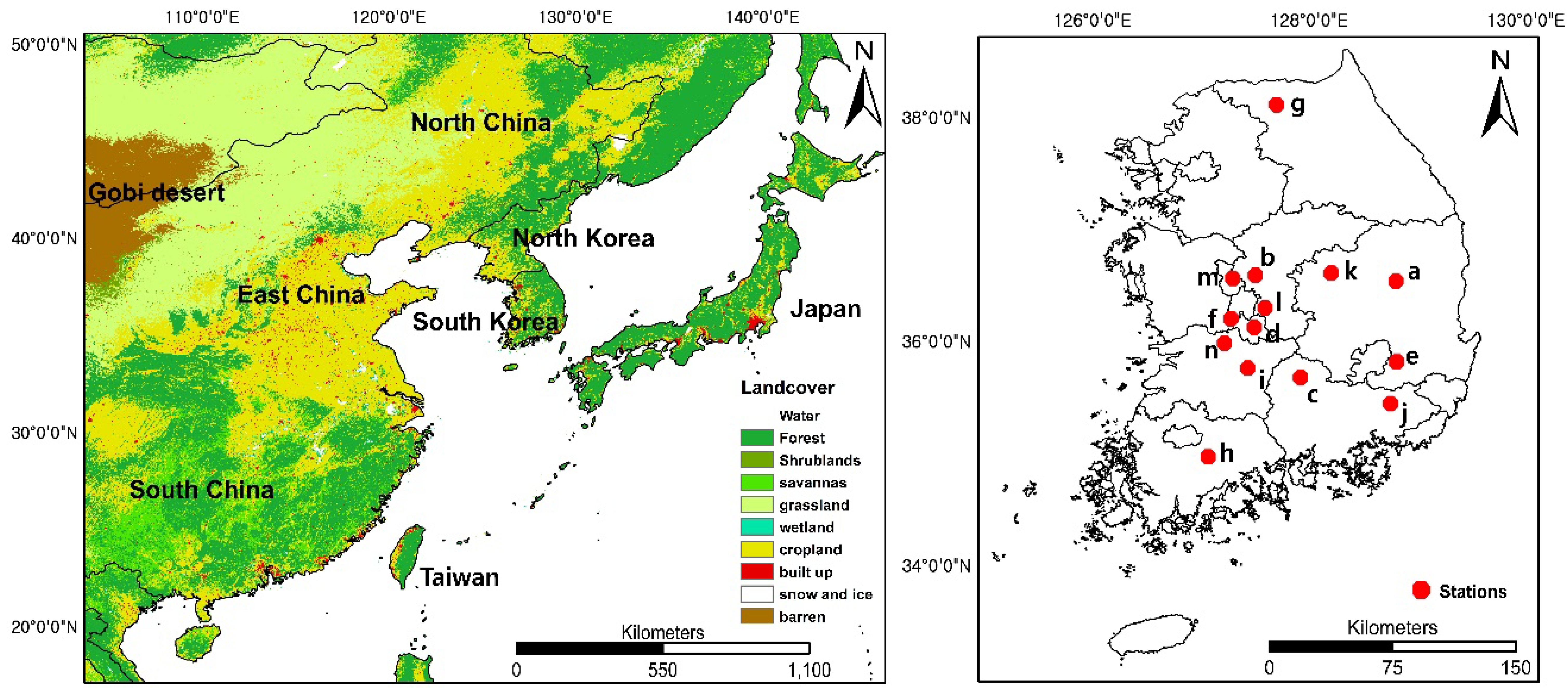
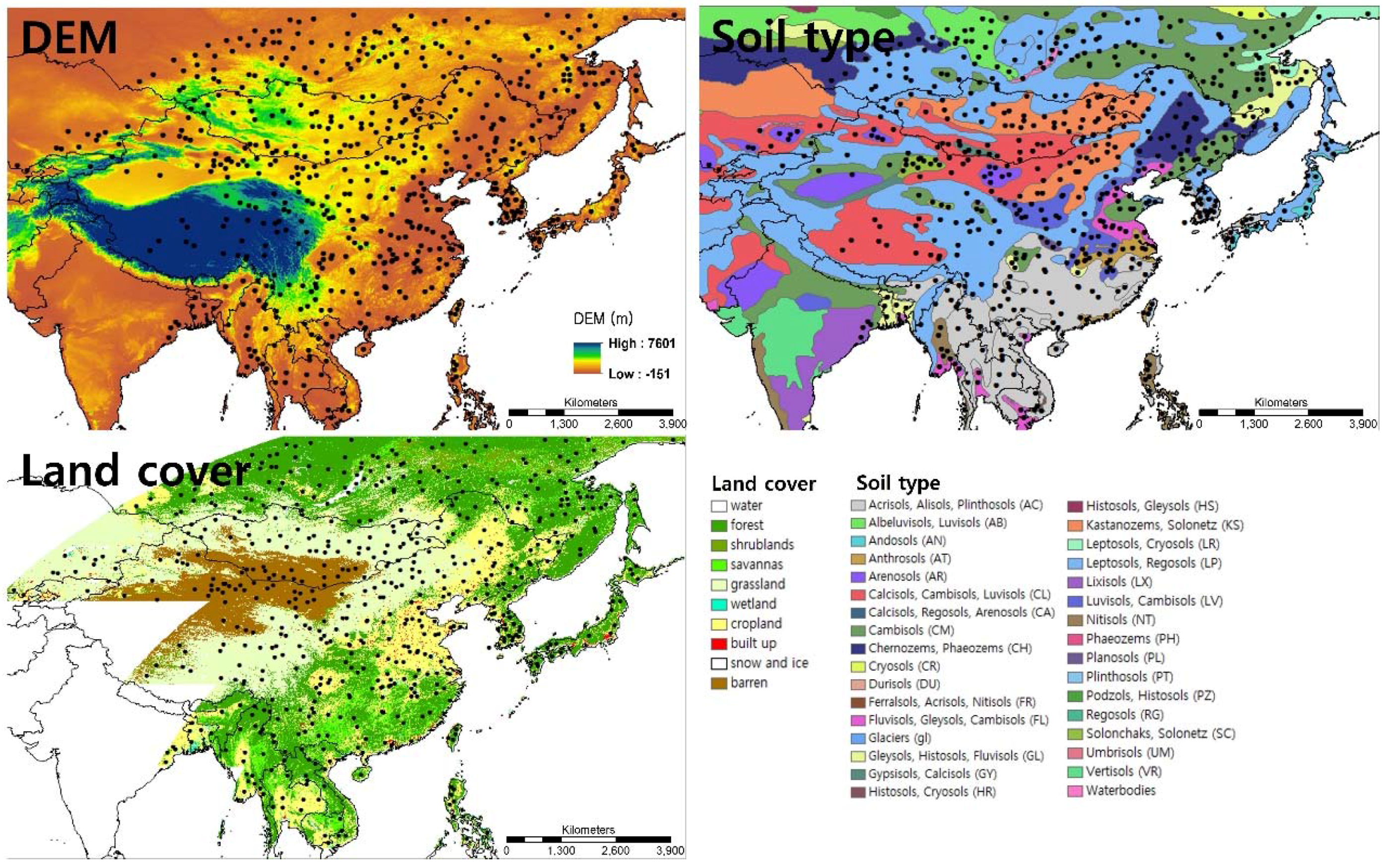
The study area is East Asia (latitude: 10.17° N–46.72° N; longitude: 106.05° E–178.25° E), including east China, southeast Russia, Taiwan, Korea, and Japan (Figure 1). East Asia frequently suffers from floods (typically from June to August) and droughts (typically from March to May) due to the climatic characteristics of the region such as monsoons. East Asia has generally hot and humid weather conditions in summer, while it is dry and cold in winter. Climatic characteristics such as mean temperature and precipitation are slightly different from country to country (in particular by latitude). The annual mean temperature is about 15 °C in East China, 12 °C on the Korean peninsula, and 16 °C in Japan. Figure 1 shows the land cover distribution of the study area. East China consists of forest, cropland, savannas, grassland, and barren areas, and the Korean peninsula and Japan are mostly composed of forest and cropland. There are 15 soil types in the study area. While most of these different soil types are found in east China, only two (i.e., leptosols and acrisols) exist in Korea and three (i.e., leptosols, acrisols, and andosols) in Japan.
2.2. Satellite Data
2.2.1. Soil Moisture
The AMSR2 instrument on the Global Change Observing Mission—Water (GCOM-W) satellite launched in 2012, extends the legacy of AMSR-E. Compared to AMSR-E, AMSR2 has improved characteristics such as mitigating radio frequency interference (RFI) using an additional channel (C-band frequency), higher reliability, and an improved calibration system [64,65,66,67]. The AMSR2 C-band-derived daily soil moisture product provided by the Japan Aerospace Exploration Agency (JAXA) at 0.1 and 0.25 degrees spatial resolution by percent of volumetric water ranging from 0 to 40% was used in this study. The product is retrieved by calculating the Polarization Index (PI) and the Index of Soil Wetness (ISW) using 10 and 36 GHz brightness temperature defined by Equations (1) and (2) based on a look-up-table approach [18].
ASCAT on the Meteorological operational satellite-A (MetOp-A) satellite is a real aperture radar sensor measuring radar backscatter using the C-band for monitoring wind over the oceans, soil moisture, and vegetation [68]. ASCAT soil moisture data sensed by C-band (5.255 GHz) microwaves from 2013 to 2015 were obtained from the European Organization for the Exploitation of Meteorological Satellites (EUMETSAT; http://www.eumetsat.int). The soil moisture was calculated from backscattered data by using Equation (3) [69,70].
2.2.2. Other Input Parameters
MODIS is an instrument onboard Terra and Aqua satellites, which has been widely used for various environmental monitoring applications on both regional and global scales. The eight-day LST (MOD11A2) [71], 16-day NDVI (MOD13A2) [72], and Land cover (MCD12Q1) [73] Terra ascending data (10:30 am) were used in this study (Table 1). While LST and NDVI are provided a 1 km resolution, the land cover product (MCD12Q1) has a spatial resolution of 500 m. The land cover data with seventeen classes was resampled to 1 km using a majority filter, and then the similar classes were aggregated to nine classes. Since the accuracy of MODIS land cover is not high for all classes especially for vegetation (e.g., Forest, Shrublands, and Savannas) in East Asia, we used representative land covers through the aggregation of similar classes (refer to the Appendix A Table A1). A total of 24 tiles (h23v03 to h30v07) covering the study area from 2013 to 2015 were obtained from the reverb echo site (http://reverb.echo.nasa/gov/reverb).
The Shuttle Radar Topography Mission (SRTM) [74] was flown on the Space Shuttle mission Endeavour STS-99, which had C-band Spaceborne Imaging Radar and X-band Synthetic Aperture Radar (X-SAR) hardware. A near-global Digital Elevation Model (DEM) was obtained using the interferometric processing of single pass data [75]. SRTM DEM data is provided at 30 m and 90 m resolution from the United States Geological Survey (USGS) Elevation Products site (http://eros.usgs.gov/elevation-products). In this study, 90 m DEM data was used and resampled using a mean function to 1 km; the same as MODIS products.
2.3. Reference Data
2.3.1. GLDAS Soil Moisture
GLDAS has been developed to identify land surface states and fluxes using data assimilation techniques and consists of three land surface models; Mosaic, Noah, and the Community Land Model (CLM) [25,76]. GLDAS soil moisture data from 2013 to 2015 was archived from Goddard Earth Sciences Data and Information Services Center (http://disc.sci.gsfc.nasa.gov/hydrology/data-holdings). In this study, three-hourly GLDAS Noah Land Surface Model (LSM) data at the spatial resolution of 0.25 degrees was used because GLDAS Noah LSM provides higher resolution data among GLDAS soil moisture products. Specifically layer 1 (i.e., 1–10 cm) soil moisture data was used because satellite-derived soil moisture involves only top soil moisture (1–5 cm). Since daily soil moisture data is not provided, daily soil moisture was calculated by averaging three-hourly data.
2.3.2. Ground Soil Moisture
Ground soil moisture data at 14 stations in South Korea were obtained from the Korea Rural Development Administration (RDA; http://weather.rda.go.kr/). RDA provides hourly ground soil moisture data in percentage at 10 cm depth using Time Domain Reflectometry (TDR) which is based on the relation between dielectric properties of soils and moisture levels [77]. Table 2 shows information on about 14 stations such as location, elevation, and land cover. Most of the stations are located in cropland, and the soil types are mainly sandy loam, clay, and clay loam. In this study, daily soil moisture data was calculated by averaging hourly data at each station to evaluate downscaled GLDAS and satellite-derived soil moisture data.
3. Methodology
A total of six input variables, ASCAT soil moisture, AMSR2 soil moisture, MODIS LST, NDVI, and Land Cover, and SRTM DEM, were used for simulation of the GLDAS soil moisture to develop a machine learning-based soil moisture downscaling algorithm. Although Tropical Rain Measuring Mission (TRMM) precipitation was originally considered as an input variable in this study, it was excluded based on the preliminary results, which did not produce improvement in performance (not shown). In addition, TRMM data was not available for the northern part (>50 degrees) of the study region. The high uncertainty of TRMM precipitation over high latitudes (>40 degrees) may be the reason for its poor contribution to the soil moisture downscaling. Figure 2 shows the process flow diagram proposed in the study. First, MODIS products and SRTM DEM were aggregated to the same grid size with GLDAS soil moisture (25 km) using a mean function. Six inputs at 25 km grid size from 2013 to 2015 (i.e., daily except for DEM and Land Cover) were extracted based on 602 point locations that were selected after considering soil type, land cover, and DEM distribution throughout East Asia. The spatial distribution of the selected points and their characteristics in terms of the three considerations (i.e., soil type, land cover, and DEM) are summarized in Appendix A Figure A1 and Table A2. Although AMSR2, ASCAT, and GLDAS provide daily products, the MODIS LST and NDVI were provided with eight-day and 16-day intervals, respectively. The same values of MODIS LST and NDVI were used during the intervals corresponding to daily products. A total of 36,412 samples for clear sky days were used to develop the downscaling algorithm. The samples from 2013 to 2014 were used as training data (n = 20,787), and validation was conducted using the samples in 2015 (n = 15,625). This hindcast validation approach is commonly used in the operational applications of satellite remote sensing, especially for meteorological applications [51,78,79,80,81]. Six independent variables, ASCAT, AMSR2, MODIS, and SRTM products, and the dependent variable of GLDAS soil moisture were fed into machine learning (dotted lines in Figure 2).
We adopted a modified regression tree from Cubist after considering the performance and operational use of the approach based on our previous study [32]. Although random forest proved to be very robust in many remote sensing applications [82,83,84,85] and produced slightly better performance in Im et al. [32], it requires a much longer processing time than a modified regression tree, i.e., Cubist, which is not appropriate for operational use. Cubist regression trees developed by RuleQuest Research have been widely used in the remote sensing field [32,49,86,87,88]. Cubist regression trees consider the nonlinear relationships between independent and dependent variables for modeling, and both continuous and discrete variables are allowed as input [89]. Tree output from the Cubist approach consists of rules and multivariate regression associated with each rule to estimate the dependent variable, which is straightforward and interpretable. Thus, it overcomes the limitations of simple linear models [90]. Relative variable importance in Cubist models can be identified based on the percentage of variable usage in rules and regression models. Rules can be generated up to 500 in Cubist models, and the number of rules is controllable using a pruning approach by limiting the maximum number of rules. Cubist regression trees generate the optimum number of rules that is less than the maximum number of rules specified by the user. In this study, the number of rules was optimized based on the pruning approach using Root Mean Square Error (RMSE) and correlation coefficients (r). Finally, an optimized regression tree to estimate GLDAS soil moisture was determined. It is relatively easy to understand the physical meanings of resultant rules, and this approach has shorter operation time than other machine learning approaches such as random forest.
Since the spatial resolution of AMSR2 and ASCAT soil moisture products is 25 km, they were resampled to a 1 km grid size simply by using the triangle-based linear interpolation in MATLAB, commonly used for the resampling of gridded data. We expected that the performance of the soil moisture downscaling model could be improved by incorporating AMSR2 and ASCAT soil moisture data, which provide basic information on soil moisture in spite of their coarse resolution, because our study area (East Asia) is wide and heterogeneous in terms of topography, land cover, and climate conditions. In order to evaluate the model performance, r, RMSE, root-mean-squared difference (RMSD), relative RMSE (rRMSE), or relative RMSD (rRMSD) were used. Downscaled 1 km soil moisture data was quantitatively compared with the in situ soil moisture data.
4. Results and Discussion
4.1. Model Optimization
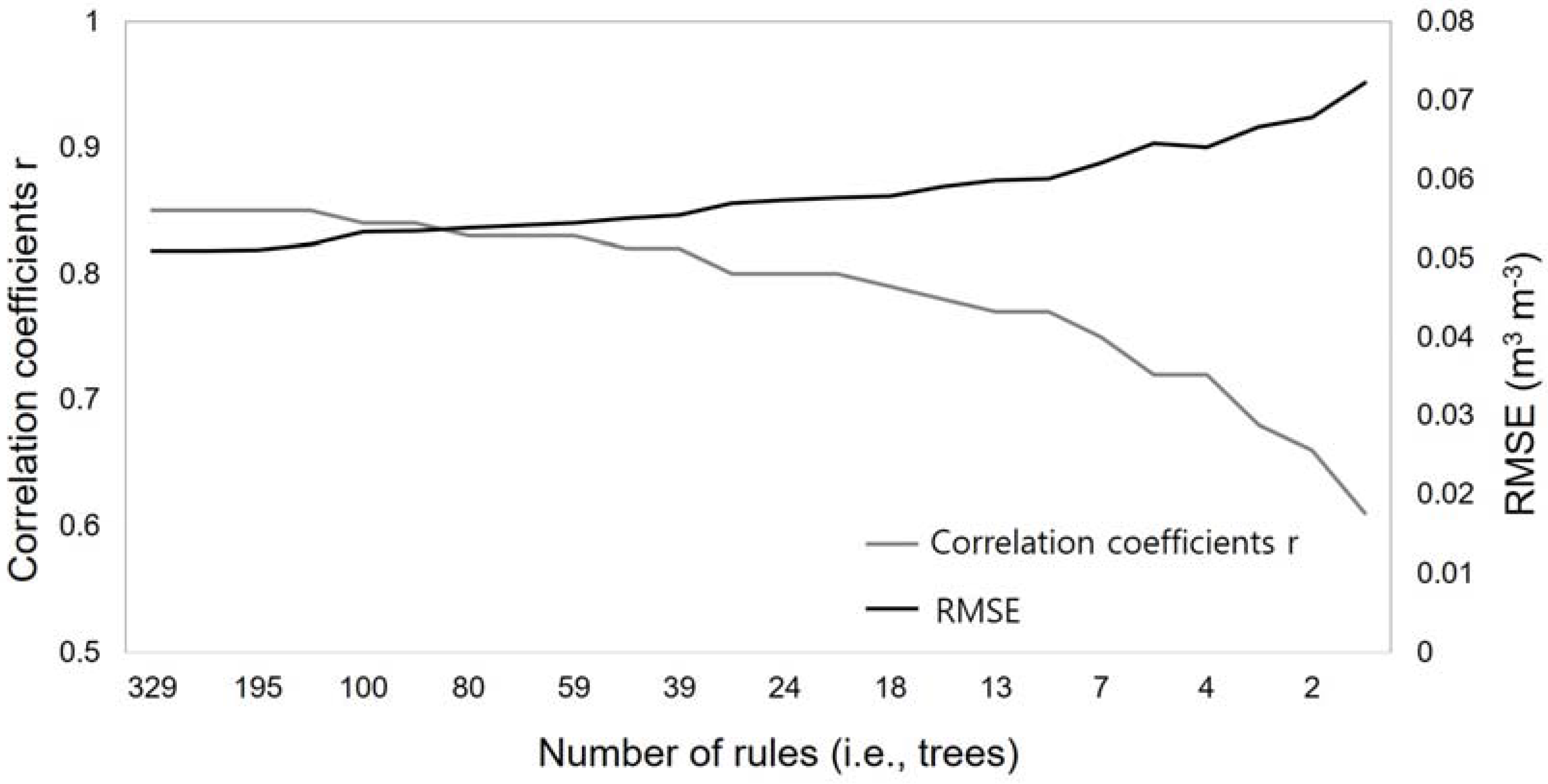
The maximum number of rules from the fully grown regression tree generated in this study was 329. The optimization of the number of rules was conducted using the validation dataset (n = 15,625) based on the accuracy metrics, RMSE and r. A smaller numbers of rules was produced through the pruning process. Figure 3 shows the change of the RMSE and r values with the decreasing number of rules. As expected, the larger number of rules produced the lower RMSE and the higher r. However, there was no significant difference in RMSE and r for the relatively large numbers of rules (≥59). For numbers of rules smaller than 59, RMSE dramatically increased with the decreasing number of rules. As the number of rules decreased, most of rules became simplified and aggregated into smaller numbers of rules. In this study, we determined 59 to be the optimal number of rules. Each rule is associated with a multivariate regression model, which has been commonly used in the literature [37,38,41,42]. The modified regression tree (Figure 3; RMSE = 0.06 m3·m−3, r = 0.8) showed better modeling performance than the single multiple linear regression model (Figure 3; RMSE = 0.07 m3·m−3, r = 0.6).
Table 3 summarizes the sub-models selected from the optimized regression tree results (i.e., 59 rule-based sub-models), which covered the majority of sample cases to downscale GLDAS soil moisture in this study. Each sub-model consists of a rule and its associated multivariate regression model. Since land cover is a discrete variable, land cover was used only for the rules. East Asia has various geophysical characteristics in terms of topography, land cover, and seasonal climate conditions. The downscaling model considered such geographical and seasonal characteristics in the rules in that the elevation (DEM), surface temperature (LST), land cover type, and vegetation healthiness (NDVI) were used to identify geographical and seasonal characteristics. Each rule provides specific conditions with thresholds so that the corresponding multivariate regression can be applied. For example, rule 1 estimated dry soil moisture (mean = 0.13 m3·m−3) in a barren area with high LST, while rule 40 was used to estimate wet soil moisture (mean = 0.29 m3·m−3) in an area of vegetation (forest, shrublands, savannas, and cropland) with low LST and high NDVI. In this case, rule 2 (mean = 0.14 m3·m−3) and rule 3 (mean = 0.16 m3·m−3) have the same conditions for land cover and LST, but they have different conditions for ASCAT, DEM, and NDVI. Rule 3 was developed to estimate slightly wetter soil moisture than rule 2, so the condition of ASCAT soil moisture (ASCAT > 0.1713) in rule 3 is higher than in rule 2 (ASCAT ≤ 0.1713).
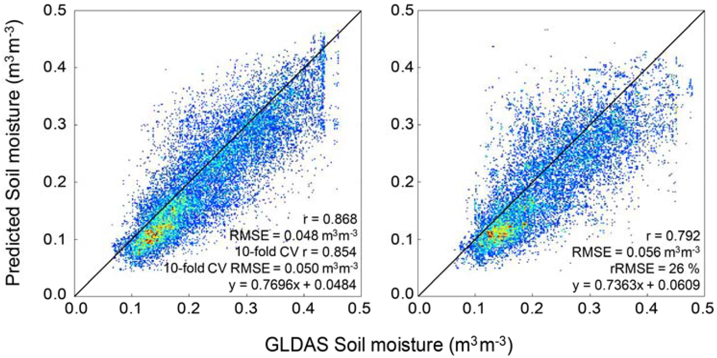
Figure 4 depicts the modeling results (i.e., both calibration and validation) of the optimized regression tree (59 rules) that compare the predicted soil moisture with the GLDAS soil moisture. Calibration and validation were conducted using the training dataset (2013–2014) and the test dataset (2015), respectively. The modeling performance was good in both calibration (r = 0.87, RMSE = 0.048 m3·m−3, and slope = 0.77) and validation (r = 0.79, RMSE = 0.056 m3·m−3, and slope = 0.74), although the validation results were slightly poorer than those in the calibration. The proposed downscaling model seems to underestimate GDLAS soil moisture.
Table 4 shows the attribute usage information of the six variables in the rules and regression models. Land cover, DEM, and LST show high usage (~80–90%) in the rules because they are important variables to distinguish regional and seasonal characteristics of soil moisture in East Asia. Five variables, except for land cover, were evenly used in the regression models, with the usage ranging from 74 to 97%. It is not surprising that DEM, LST, land cover, and NDVI show high variable importance since such information is integrated when producing the GLDAS soil moisture. It is surprising, though, that the soil moisture products from ASCAT and AMSR2 were not more frequently used in the rules than the other variables to estimate GLDAS soil moisture. This implies that ASCAT and AMSR2 soil moisture algorithms might not be able to effectively consider regional or seasonal characteristics in East Asia. When ASCAT and AMSR2 soil moisture data were compared to GLDAS soil moisture, ASCAT data tended to overestimate soil moisture, while AMSR2 data significantly underestimated soil moisture throughout the study area. This may explain the low usage of the ASCAT and AMSR2 data (especially AMSR2) to simulate GLDAS soil moisture in both the rules and regression models that resulted from the modified regression tree.
4.2. Model Evaluation
Figure 5 shows the time series of ground soil moisture, GLDAS soil moisture, and 1 km downscaled soil moisture with precipitation at 14 stations during growing season (from May to September) in 2015. Since the 1 km downscaled soil moisture cannot be produced under cloudy days due to missing data for input variables, there are some gaps in Figure 5. The 1 km downscaled soil moisture, as well as GLDAS soil moisture, show a similar temporal pattern to ground soil moisture. Soil moisture increased with increasing rainfall. Soil moisture is generally low in the dry season and high in the wet season. However, GLDAS and the 1 km downscaled soil moisture tend to be underestimated when compared to ground soil moisture, as discussed by Zhang et al. [76], due to the difference between the depth of GLDAS and the 1 km downscaled soil moisture (~5 cm) and ground soil moisture (10 cm). It should also be noted that the spatial scales are quite different among the three types of soil moisture data: ground soil moisture was measured at point locations, while GLDAS and 1 km downscaled soil moisture data were observed over 25 km × 25 km and 1 km × 1 km grids, respectively. Thus, while ground soil moisture fluctuates highly, GLDAS soil moisture data does not relatively show extreme values. As discussed in Choi et al. [37], although most RDA sites are located in cropland, the corresponding domains of AMSR-E (25 km) and MODIS (1 km) for each site consist of more heterogeneous land cover types (e.g., cropland, built-up, barren land, and forest) because the RDA sites were not initially designed to validate remote sensing soil moisture. On the other hand, many validation sites in previous studies were designed considering remote sensing validation and consist of homogeneous land cover within remote sensing pixels such as OZnet [91,92].
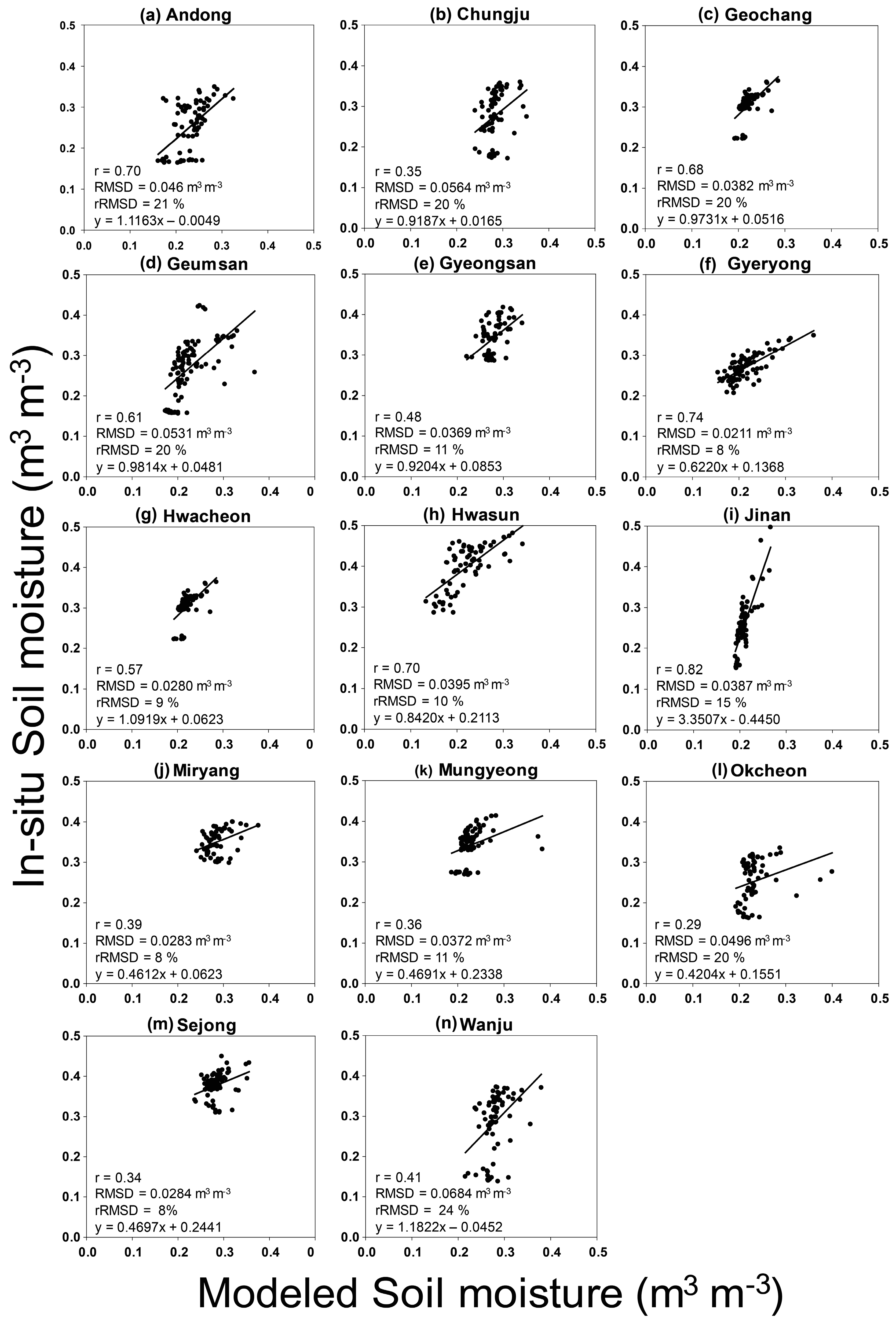
The 1 km downscaled soil moisture was compared to the ground soil moisture using scatterplots at 14 stations from May to September 2015 (Figure 6). Since ground soil moisture has a spatial scale different from the downscaled one, ground soil moisture within each grid (i.e, 1 km × 1 km) was assumed to be consistent [32]. The comparison between the ground and downscaled soil moisture data varied by station resulting in mean slope ~ 0.987, mean RMSD ~ 0.041 m3·m−3, and mean r ~ 0.53 from all 14 stations. The 1 km downscaled soil moisture produced in this study also shows relatively low RMSD and high r compared to other soil moisture downscaling studies from Im et al. [32] (resulting in the mean slope = 0.366, mean RMSD = 0.092 m3·m−3, and mean r = 0.51), Choi et al. [37] (resulting in the mean slope = 0.769, mean RMSD = 0.124 m3·m−3, and mean r = 0.46), Merlin et al. [93] (resulting in the mean slope = 0.523, mean RMSD = 0.078 m3·m−3, and mean r = 0.58), and Djamai et al. [94] (resulting in the mean slope = 1.188, mean RMSD = 0.07 m3·m−3, and mean r = 0.5), although it is not possible to directly compare the accuracy metrics among the studies. Nonetheless, the results imply that the high-resolution soil moisture produced using the proposed downscaling approach is closely related to ground soil moisture.
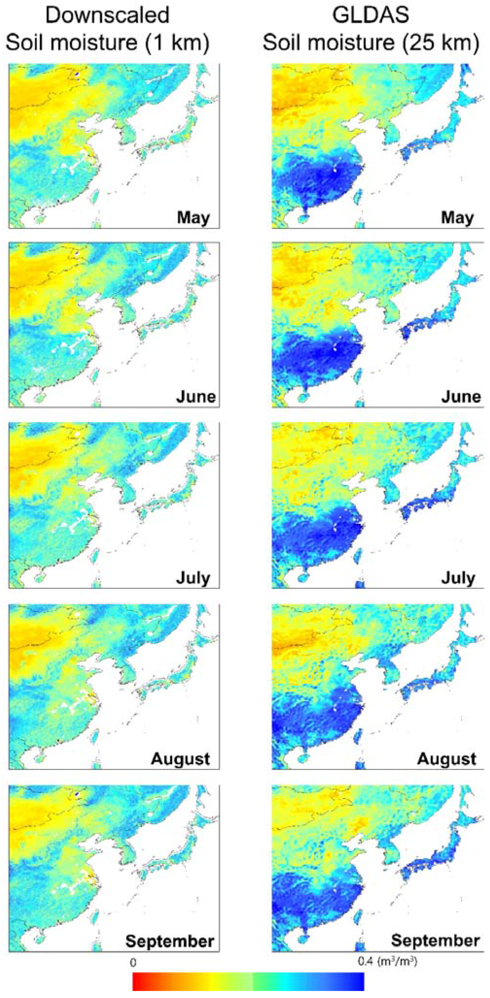
Figure 7 shows the spatial distribution of monthly downscaled and GLDAS soil moisture from May to September in 2015. The spatial distributions of both soil moisture data by land cover are consistent with the literature [95,96]. Both soil moisture products show relatively high soil moisture levels in forest regions (i.e., southern China, Korea Peninsula, and Japan), while presenting dry soil in desert and built up regions (i.e., Shandong, Gobi Desert). North China, including the Gobi Desert, has low soil moisture conditions regardless of the season. The 1 km downscaled soil moisture over some parts in southern China was not available due to clouds, and it shows quite different conditions compared to GLDAS soil moisture. The much smaller number of training samples (less than 8% among the total number of training samples) over southern China may explain such poor performance, which implies that the performance of the empirical model highly depends on the number of training samples. The dynamic range of the predicted soil moisture was slightly smaller (~0.05 m3·m−3) than the GLDAS soil moisture because the Cubist model tends to produce results to reduce estimation errors similar to other empirical statistical and machine learning approaches, which leads to a smaller dynamic range toward mean values [32,49]. While the 1 km downscaled soil moisture was underestimated in humid regions (e.g., Japan, North Korea, and Taiwan), it was overestimated in dry regions (e.g., the Gobi Desert) when compared to GLDAS soil moisture. However, the spatial pattern of the 1 km downscaled soil moisture was well matched with GLDAS soil moisture. Both soil moisture products also show a similar temporal pattern that is relatively dry in spring (May and June), with a large portion of the Gobi Desert, and relatively wet in summer (July and August), with a small portion of the desert. Daily 1 km downscaled and GLDAS soil moisture data during the growing season (May to September 2015; 153 days) were compared using r and RMSE (Figure 8). It should be noted that positive correlation (0.353 averaged) and low RMSE (<0.06 m3·m−3) appear in most areas. Cloudy regions such as southern China and southern Japan showed lower r and higher RMSE than other regions due to the limited number of training samples. The northeastern part of the study region has negative correlation, which implies that the downscaling model was not able to capture the soil moisture pattern in the area. Unlike the other areas, soil moisture in this part has a very small dynamic range (~0.1 m3·m−3) during the growing season, which possibly resulted in low correlation coefficients when the downscaled soil moisture data was compared to GLDAS soil moisture information. Although the topographic and land cover characteristics of this area are similar to those in the northern part of North Korea, the soil moisture pattern is a bit different between the two areas. Unlike the sufficient number of training samples selected in North Korea that were used to develop the downscaling model, limited training samples from the northeastern part of the study region may also explain the negative correlation between the downscaled and the GLDAS soil moisture data.
4.3. Novelty, Opportunities, and Limitations
This study developed a soil moisture downscaling model, considering its operational use. Although different machine learning approaches such as random forest may result in higher modeling accuracy to downscale soil moisture [32], they require more computational demand (about 13 times) to produce high resolution soil moisture over a large area (e.g., East Asia). The computational cost is important for the operational use of a model. While it took 15 min to produce the 1 km downscaled soil moisture map over East Asia (9600 × 6000 grids) when using the optimized regression tree, it took 3 h 25 min when using random forest with the hardware environment of Intel Core i7-4770 CPU @ 3.4GHz (Hewlett Packard, Palo Alto, CA, USA) and MATLAB 2016b (Mathworks, Natick, MA, USA).
It is also difficult to interpret the model, including the physical meaning and the process when using random forest, which uses hundreds of trees. The optimized regression tree provides explicit rules and regression models, shows high performance, and produces soil moisture data faster than random forest. Figure 9 shows the spatial distributions of the daily downscaled soil moisture and TRMM precipitation from 10 to 16 July 2015. There were heavy rains between 11 and 12 July over the Korean peninsula. The heavy rainfall caused the increase in soil moisture from 11 July to 14 July (peak). Since there was no precipitation after 14 July, the soil moisture decreased (15–16 July). The daily downscaled soil moisture produced in this study well reflects the changes in precipitation. Therefore, it can be seen that the optimized regression tree is very useful in producing valid soil moisture data with a high resolution.
There are some limitations in this study. Although this approach produced daily soil moisture data that was well matched with both in situ and GLDAS soil moisture data, there are many no-data regions (e.g., southern China) due to cloud cover, especially during the wet season. Since our study period was from 2013 to 2015, we were unable to use other remote sensing data from recently launched satellites such as Global Precipitation Measurement (GPM) and SMAP. The use of the small number of input variables (i.e., six) considering the operational efficiency of the model is another limitation.
5. Conclusions
This study aims to develop a soil moisture downscaling model by optimizing a modified regression tree for operational use. The optimized regression tree that consists of 59 rules and regression models produces daily high resolution (1 km) real time soil moisture data in East Asia using MODIS, ASCAT, AMSR2, and SRTM products. The 1 km downscaled soil moisture showed high correlation and low RMSE when compared to GLDAS soil moisture. Ground soil moisture data at 14 stations was also used to assess the 1 km downscaled soil moisture. The 1 km downscaled soil moisture moderately correlated with ground soil moisture and was closely related to the variations in precipitation. The spatiotemporal distributions of the 1 km downscaled soil moisture was also well matched with those of the GLDAS soil moisture data. This implies that the downscaled soil moisture may provide valuable information for identifying agricultural and hydrological processes such as drought monitoring at various spatial scales.
Our study has some limitations that should be improved upon in further research. Since some of the input parameters were from optical sensor data, there was a no-data problem due to clouds. This can be improved by adopting a hierarchical approach, i.e., applying another model without using optical sensor data for cloud pixels. Similar to other empirical approaches, regression trees tend to result in a reduced dynamic range of a target variable (i.e., soil moisture in this study) toward the mean [32]. Another limitation is that the model did not use other recent remote sensing data such as GPM and SMAP due to the study period (from 2013 to 2015) and computational demand, considering the operational use of the proposed model. In future research, additional data will be incorporated to improve the performance of the high resolution soil moisture model. Cumulative distribution function (CDF) matching will be also applied to downscaled soil moisture data so that it has a similar dynamic range to GLDAS soil moisture. The proposed method will be tested for different regions such as Africa and Europe to examine the feasibility of the proposed approach to the production of global high resolution soil moisture data.
Acknowledgments
This research was supported by ‘The development of satellite data utilization and Operation supportive technology’ of the National Meteorological Satellite Center (NMSC)/KMA. This research was also supported by the Space Technology Development Program and the Technology Development Program to Solve Climate Changes through the National Foundation of Korea (NRF), funded by the Ministry of Science, ICT, and Future Planning of Korea (Grant: NRF-2014M1A3A3A03034799; NRF-2012M1A2A2671851).
Author Contributions
Seonyoung Park and Sumin Park led manuscript writing and contributed to the data analysis and research design. Jungho Im supervised this study, contributed to the research design and manuscript writing, and served as the corresponding author. Jinyoung Rhee, Jinho Shin, and Jun Dong Park contributed to the discussion of the results and manuscript writing.
Conflicts of Interest
The authors declare no conflict of interest.
Appendix A

Table A1.
Land cover aggregation from seventeen classes to nine by grouping similar classes.
| Original Class | Original Land Cover | New Class | Aggregated Land Cover |
|---|---|---|---|
| 0 | Water | 0 | Water |
| 1 | Evergreen Needleleaf forest | 1 | Forest |
| 2 | Evergreen Broadleaf forest | 1 | Forest |
| 3 | Deciduous Needleleaf forest | 1 | Forest |
| 4 | Deciduous Broadleaf forest | 1 | Forest |
| 5 | Mixed forest | 1 | Forest |
| 6 | Closed shrublands | 2 | Shrublands |
| 7 | Open shrublands | 2 | Shrublands |
| 8 | Woody savannas | 3 | Savannas |
| 9 | Savannas | 3 | Savannas |
| 10 | Grasslands | 4 | Grasslands |
| 11 | Permanent wetlands | 5 | Permanent wetlands |
| 12 | Croplands | 6 | Croplands |
| 13 | Urban and built-up | 7 | Urban and built-up |
| 14 | Cropland/Natural vegetation mosaic | 6 | Cropland |
| 15 | Snow and ice | 8 | Snow and ice |
| 16 | Barren or sparsely vegetated | 4 | Grasslands |
Table A2.
The percentage of area and the selected sampling points (602 points) for each class in Digital Elevation Model (DEM), land cover, and soil type within the study area.
Table A2.
The percentage of area and the selected sampling points (602 points) for each class in Digital Elevation Model (DEM), land cover, and soil type within the study area.
| DEM | Range (m) | Area (%) | Points (%) |
| −151 ≤ DEM < −1 | 0.026 | 0.17 | |
| −1 ≤ DEM < 0 | 0.45 | 0.66 | |
| 0 ≤ DEM < 120 | 14.98 | 15.78 | |
| 120 ≤ DEM < 340 | 20.41 | 13.79 | |
| 340 ≤ DEM < 710 | 21.15 | 19.93 | |
| 710 ≤ DEM < 1110 | 14.14 | 16.78 | |
| 1110 ≤ DEM < 7601 | 28.84 | 32.89 | |
| Land cover | Class | Area (%) | Points (%) |
| Water | 47.14 | 1.99 | |
| Forest | 18.11 | 30.07 | |
| Shrublands | 0.26 | 4.15 | |
| Savannas | 1.25 | 6.15 | |
| Grassland | 12.88 | 21.93 | |
| Wetland | 0.29 | 0.66 | |
| Cropland | 17.23 | 23.59 | |
| Built up | 0.81 | 1.33 | |
| Snow and ice | 0.01 | 0.50 | |
| Barren | 2.02 | 9.63 | |
| Soil type | Soil Type | Area (%) | Points (%) |
| Waterbodies | 0.06 | 1.00 | |
| Calcisols, Cambisols, Luvisols | 5.76 | 7.14 | |
| Arenosols | 0.14 | 3.16 | |
| Andosols | 1.67 | 1.50 | |
| Leptosols, Regosols | 22.62 | 20.43 | |
| Anthrosols | 2.97 | 2.82 | |
| Fluvisols, Gleysols, Cambisols | 3.16 | 3.65 | |
| Gleysols, Histosols, Fluvisols | 3.21 | 3.65 | |
| Chernozems, Phaeozems | 7.37 | 3.99 | |
| Planosols | 0.39 | 0.50 | |
| Cambisols | 8.55 | 13.29 | |
| Kastanozems, Solonetz | 15.65 | 9.30 | |
| Acrisols, Alisols, Plinthosols | 20.89 | 13.12 | |
| Luvisols, Cambisols | 6.70 | 5.32 | |
| Ferralsols, Acrisols, Nitisols | 0.01 | 0.66 | |
| Nitisols | 0.83 | 1.99 |
Figure A1.
Spatial distribution of the selected sampling points (i.e., 602 points) considering DEM, soil type, and land cover.
Figure A1.
Spatial distribution of the selected sampling points (i.e., 602 points) considering DEM, soil type, and land cover.

References
- Seneviratne, S.I.; Lüthi, D.; Litschi, M.; Schär, C. Land–atmosphere coupling and climate change in Europe. Nature 2006, 443, 205–209. [Google Scholar] [CrossRef] [PubMed]
- Buma, W.G.; Lee, S.-I.; Seo, J.Y. Hydrological evaluation of Lake Chad basin using space borne and hydrological model observations. Water 2016, 8, 205. [Google Scholar] [CrossRef]
- Schär, C.; Lüthi, D.; Beyerle, U.; Heise, E. The soil–precipitation feedback: A process study with a regional climate model. J. Clim. 1999, 12, 722–741. [Google Scholar] [CrossRef]
- Spence, C.; Kokelj, S.A.; Kokelj, S.V.; Hedstrom, N. The process of winter streamflow generation in a subarctic Precambrian Shield catchment. Hydrol. Process. 2014, 28, 4179–4190. [Google Scholar] [CrossRef]
- Anderson, M.; Norman, J.; Diak, G.; Kustas, W.; Mecikalski, J. A two-source time-integrated model for estimating surface fluxes using thermal infrared remote sensing. Remote Sens. Environ. 1997, 60, 195–216. [Google Scholar] [CrossRef]
- Idso, S.; Jackson, R.; Reginato, R.; Kimball, B.; Nakayama, F. The dependence of bare soil albedo on soil water content. J. Appl. Meteorol. 1975, 14, 109–113. [Google Scholar] [CrossRef]
- Jiang, Y.; Weng, Q. Estimation of hourly and daily evapotranspiration and soil moisture using downscaled LST over various urban surfaces. GISci. Remote Sens. 2017, 54, 95–117. [Google Scholar] [CrossRef]
- Dursun, M.; Ozden, S. A wireless application of drip irrigation automation supported by soil moisture sensors. Sci. Res. Essays 2011, 6, 1573–1582. [Google Scholar]
- Qi, Z.; Zhang, T.; Zhou, L.; Feng, H.; Zhao, Y.; Si, B. Combined Effects of Mulch and Tillage on Soil Hydrothermal Conditions under Drip Irrigation in Hetao Irrigation District, China. Water 2016, 8, 504. [Google Scholar] [CrossRef]
- Dai, A.; Trenberth, K.E.; Qian, T. A global dataset of Palmer Drought Severity Index for 1870–2002: Relationship with soil moisture and effects of surface warming. J. Hydrometeorol. 2004, 5, 1117–1130. [Google Scholar] [CrossRef]
- Martínez-Fernández, J.; González-Zamora, A.; Sánchez, N.; Gumuzzio, A.; Herrero-Jiménez, C. Satellite soil moisture for agricultural drought monitoring: Assessment of the SMOS derived Soil Water Deficit Index. Remote Sens. Environ. 2016, 177, 277–286. [Google Scholar] [CrossRef]
- Otkin, J.A.; Anderson, M.C.; Hain, C.; Svoboda, M.; Johnson, D.; Mueller, R.; Tadesse, T.; Wardlow, B.; Brown, J. Assessing the evolution of soil moisture and vegetation conditions during the 2012 United States flash drought. Agric. For. Meteorol. 2016, 218, 230–242. [Google Scholar] [CrossRef]
- Wang, H.; Vicente-Serrano, S.M.; Tao, F.; Zhang, X.; Wang, P.; Zhang, C.; Chen, Y.; Zhu, D.; El Kenawy, A. Monitoring winter wheat drought threat in Northern China using multiple climate-based drought indices and soil moisture during 2000–2013. Agric. For. Meteorol. 2016, 228, 1–12. [Google Scholar] [CrossRef]
- Stéfanon, M.; Drobinski, P.; D’Andrea, F.; Lebeaupin-Brossier, C.; Bastin, S. Soil moisture-temperature feedbacks at meso-scale during summer heat waves over Western Europe. Clim. Dyn. 2014, 42, 1309–1324. [Google Scholar] [CrossRef]
- Padhee, S.K.; Nikam, B.R.; Dutta, S.; Aggarwal, S.P. Using satellite-based soil moisture to detect and monitor spatiotemporal traces of agricultural drought over Bundelkhand region of India. GISci. Remote Sens. 2017, 54, 144–166. [Google Scholar] [CrossRef]
- Wang, X.; Chen, N.; Chen, Z.; Yang, X.; Li, J. Earth observation metadata ontology model for spatiotemporal-spectral semantic-enhanced satellite observation discovery: A case study of soil moisture monitoring. GISci. Remote Sens. 2016, 53, 22–44. [Google Scholar] [CrossRef]
- Dorigo, W.; Wagner, W.; Hohensinn, R.; Hahn, S.; Paulik, C.; Xaver, A.; Gruber, A.; Drusch, M.; Mecklenburg, S.; van Oevelen, P. The International Soil Moisture Network: A data hosting facility for global in situ soil moisture measurements. Hydrol. Earth Syst. Sci. 2011, 15, 1675–1698. [Google Scholar] [CrossRef]
- Koike, T. Soil moisture. In Descriptions of GCOM-W1 AMSR2 Level 1R and Level 2 Algorithms; Japan Aerospace Exploration Agency, Earth Observation Research Center: Saitama, Japan, 2013. [Google Scholar]
- Kerr, Y.H.; Waldteufel, P.; Richaume, P.; Wigneron, J.P.; Ferrazzoli, P.; Mahmoodi, A.; Al Bitar, A.; Cabot, F.; Gruhier, C.; Juglea, S.E. The SMOS soil moisture retrieval algorithm. IEEE Trans. Geosci. Remote Sens. 2012, 50, 1384–1403. [Google Scholar] [CrossRef]
- Jackson, T.J.; Bindlish, R.; Cosh, M.H.; Zhao, T.; Starks, P.J.; Bosch, D.D.; Seyfried, M.; Moran, M.S.; Goodrich, D.C.; Kerr, Y.H. Validation of Soil Moisture and Ocean Salinity (SMOS) soil moisture over watershed networks in the US. IEEE Trans. Geosci. Remote Sens. 2012, 50, 1530–1543. [Google Scholar] [CrossRef]
- Albergel, C.; Rüdiger, C.; Carrer, D.; Calvet, J.C.; Fritz, N.; Naeimi, V.; Bartalis, Z.; Hasenauer, S. An evaluation of ASCAT surface soil moisture products with in-situ observations in Southwestern France. Hydrol. Earth Syst. Sci. 2009, 13, 115–124. [Google Scholar] [CrossRef]
- Das, N.N.; Entekhabi, D.; Njoku, E.G. An algorithm for merging SMAP radiometer and radar data for high-resolution soil-moisture retrieval. IEEE Trans. Geosci. Remote Sens. 2011, 49, 1504–1512. [Google Scholar] [CrossRef]
- Rodell, M.; Houser, P.; Jambor, U.; Gottschalck, J.; Mitchell, K.; Meng, C.; Arsenault, K.; Cosgrove, B.; Radakovich, J.; Bosilovich, M. The global land data assimilation system. Bull. Am. Meteorol. Soc. 2004, 85, 381–394. [Google Scholar] [CrossRef]
- Rienecker, M.M.; Suarez, M.J.; Gelaro, R.; Todling, R.; Bacmeister, J.; Liu, E.; Bosilovich, M.G.; Schubert, S.D.; Takacs, L.; Kim, G.-K. Merra: NASA’s modern-era retrospective analysis for research and applications. J. Clim. 2011, 24, 3624–3648. [Google Scholar] [CrossRef]
- Chen, Y.; Yang, K.; Qin, J.; Zhao, L.; Tang, W.; Han, M. Evaluation of AMSR-E retrievals and GLDAS simulations against observations of a soil moisture network on the central Tibetan Plateau. J. Geophys. Res.: Atmos. 2013, 118, 4466–4475. [Google Scholar] [CrossRef]
- Entekhabi, D.; Njoku, E.G.; O’Neill, P.E.; Kellogg, K.H.; Crow, W.T.; Edelstein, W.N.; Entin, J.K.; Goodman, S.D.; Jackson, T.J.; Johnson, J. The soil moisture active passive (SMAP) mission. Proc. IEEE 2010, 98, 704–716. [Google Scholar] [CrossRef]
- Djamai, N.; Magagi, R.; Goïta, K.; Merlin, O.; Kerr, Y.; Roy, A. A combination of DISPATCH downscaling algorithm with CLASS land surface scheme for soil moisture estimation at fine scale during cloudy days. Remote Sens. Environ. 2016, 184, 1–14. [Google Scholar] [CrossRef]
- Kim, G.; Barros, A.P. Downscaling of remotely sensed soil moisture with a modified fractal interpolation method using contraction mapping and ancillary data. Remote Sens. Environ. 2002, 83, 400–413. [Google Scholar] [CrossRef]
- Merlin, O.; Jacob, F.; Wigneron, J.-P.; Walker, J.; Chehbouni, G. Multidimensional disaggregation of land surface temperature using high-resolution red, near-infrared, shortwave-infrared, and microwave-L bands. IEEE Trans. Geosci. Remote Sens. 2012, 50, 1864–1880. [Google Scholar] [CrossRef]
- Piles, M.; Sánchez, N.; Vall-llossera, M.; Camps, A.; Martínez-Fernández, J.; Martínez, J.; González-Gambau, V. A downscaling approach for SMOS land observations: Evaluation of high-resolution soil moisture maps over the Iberian Peninsula. IEEE J. Sel. Top. Appl. Earth Obs. Remote Sens. 2014, 7, 3845–3857. [Google Scholar] [CrossRef]
- Chakrabarti, S.; Judge, J.; Bongiovanni, T.; Rangarajan, A.; Ranka, S. Disaggregation of Remotely Sensed Soil Moisture in Heterogeneous Landscapes Using Holistic Structure-Based Models. IEEE Trans. Geosci. Remote Sens. 2016, 54, 4629–4641. [Google Scholar] [CrossRef]
- Im, J.; Park, S.; Rhee, J.; Baik, J.; Choi, M. Downscaling of AMSR-E soil moisture with MODIS products using machine learning approaches. Environ. Earth Sci. 2016, 75, 1120. [Google Scholar] [CrossRef]
- Chen, N.; He, Y.; Zhang, X. NIR-Red Spectra-Based Disaggregation of SMAP Soil moisture to 250 m Resolution Based on SMAPEX-4/5 in Southeastern Australia. Remote Sens. 2017, 9, 51. [Google Scholar] [CrossRef]
- Parinussa, R.; Yilmaz, M.; Anderson, M.; Hain, C.; Jeu, R. An intercomparison of remotely sensed soil moisture products at various spatial scales over the Iberian Peninsula. Hydrol. Process. 2014, 28, 4865–4876. [Google Scholar] [CrossRef]
- Merlin, O.; Chehbouni, A.; Walker, J.P.; Panciera, R.; Kerr, Y.H. A simple method to disaggregate passive microwave-based soil moisture. IEEE Trans. Geosci. Remote Sens. 2008, 46, 786–796. [Google Scholar] [CrossRef]
- Song, C.; Jia, L.; Menenti, M. Retrieving high-resolution surface soil moisture by downscaling AMSR-E brightness temperature using MODIS LST and NDVI data. IEEE J. Sel. Top. Appl. Earth Obs. Remote Sens. 2014, 7, 935–942. [Google Scholar] [CrossRef]
- Choi, M.; Hur, Y. A microwave-optical/infrared disaggregation for improving spatial representation of soil moisture using AMSR-E and MODIS products. Remote Sens. Environ. 2012, 124, 259–269. [Google Scholar] [CrossRef]
- Piles, M.; Camps, A.; Vall-Llossera, M.; Corbella, I.; Panciera, R.; Rudiger, C.; Kerr, Y.H.; Walker, J. Downscaling SMOS-derived soil moisture using MODIS visible/infrared data. IEEE Trans. Geosci. Remote Sens. 2011, 49, 3156–3166. [Google Scholar] [CrossRef]
- Carlson, T.N.; Gillies, R.R.; Perry, E.M. A method to make use of thermal infrared temperature and NDVI measurements to infer surface soil water content and fractional vegetation cover. Remote Sens. Rev. 1994, 9, 161–173. [Google Scholar] [CrossRef]
- Carlson, T. An overview of the “triangle method” for estimating surface evapotranspiration and soil moisture from satellite imagery. Sensors 2007, 7, 1612–1629. [Google Scholar] [CrossRef]
- Chauhan, N.; Miller, S.; Ardanuy, P. Spaceborne soil moisture estimation at high resolution: A microwave-optical/IR synergistic approach. Int. J. Remote Sens. 2003, 24, 4599–4622. [Google Scholar] [CrossRef]
- Kim, J.; Hogue, T.S. Improving spatial soil moisture representation through integration of AMSR-E and MODIS products. IEEE Trans. Geosci. Remote Sens. 2012, 50, 446–460. [Google Scholar]
- Sánchez-Ruiz, S.; Piles, M.; Sánchez, N.; Martínez-Fernández, J.; Vall-llossera, M.; Camps, A. Combining SMOS with visible and near/shortwave/thermal infrared satellite data for high resolution soil moisture estimates. J. Hydrol. 2014, 516, 273–283. [Google Scholar]
- Peng, J.; Loew, A.; Merlin, O.; Verhoest, N.E.C. A review of spatial downscaling of satellite remotely sensed soil moisture. Rev. Geophys. 2017, 55. [Google Scholar] [CrossRef]
- Merlin, O.; Walker, J.P.; Chehbouni, A.; Kerr, Y. Towards deterministic downscaling of SMOS soil moisture using MODIS derived soil evaporative efficiency. Remote Sens. Environ. 2008, 112, 3935–3946. [Google Scholar] [CrossRef]
- Pelletier, C.; Valero, S.; Inglada, J.; Champion, N.; Dedieu, G. Assessing the robustness of Random Forests to map land cover with high resolution satellite image time series over large areas. Remote Sens. Environ. 2016, 187, 156–168. [Google Scholar] [CrossRef]
- Griffiths, P.; van der Linden, S.; Kuemmerle, T.; Hostert, P. A pixel-based Landsat compositing algorithm for large area land cover mapping. IEEE J. Sel. Top. Appl. Earth Obs. Remote Sens. 2013, 6, 2088–2101. [Google Scholar]
- Shao, Y.; Lunetta, R.S. Comparison of support vector machine, neural network, and CART algorithms for the land-cover classification using limited training data points. ISPRS J. Photogramm. Remote Sens. 2012, 70, 78–87. [Google Scholar] [CrossRef]
- Park, S.; Im, J.; Jang, E.; Rhee, J. Drought assessment and monitoring through blending of multi-sensor indices using machine learning approaches for different climate regions. Agric. For. Meteorol. 2016, 216, 157–169. [Google Scholar]
- Belayneh, A.; Adamowski, J.; Khalil, B.; Quilty, J. Coupling machine learning methods with wavelet transforms and the bootstrap and boosting ensemble approaches for drought prediction. Atmos. Res. 2016, 172, 37–47. [Google Scholar]
- Han, H.; Lee, S.; Im, J.; Kim, M.; Lee, M.-I.; Ahn, M.H.; Chung, S.-R. Detection of convective initiation using Meteorological Imager onboard Communication, Ocean, and Meteorological Satellite based on machine learning approaches. Remote Sens. 2015, 7, 9184–9204. [Google Scholar] [CrossRef]
- Kim, M.; Im, J.; Han, H.; Kim, J.; Lee, S.; Shin, M.; Kim, H.-C. Landfast sea ice monitoring using multisensor fusion in the Antarctic. GISci. Remote Sens. 2015, 52, 239–256. [Google Scholar] [CrossRef]
- Lee, S.; Im, J.; Kim, J.; Kim, M.; Shin, M.; Kim, H.-c.; Quackenbush, L.J. Arctic Sea Ice Thickness Estimation from CryoSat-2 Satellite Data Using Machine Learning-Based Lead Detection. Remote Sens. 2016, 8, 698. [Google Scholar] [CrossRef]
- Kühnlein, M.; Appelhans, T.; Thies, B.; Nauss, T. Improving the accuracy of rainfall rates from optical satellite sensors with machine learning—A random forests-based approach applied to MSG SEVIRI. Remote Sens. Environ. 2014, 141, 129–143. [Google Scholar] [CrossRef]
- Caicedo, J.P.R.; Verrelst, J.; Munoz-Mari, J.; Moreno, J.; Camps-Valls, G. Toward a semiautomatic machine learning retrieval of biophysical parameters. IEEE J. Sel. Top. Appl. Earth Obs. Remote Sens. 2014, 7, 1249–1259. [Google Scholar] [CrossRef]
- Ke, Y.; Im, J.; Park, S.; Gong, H. Downscaling of MODIS One kilometer evapotranspiration using Landsat-8 data and machine learning approaches. Remote Sens. 2016, 8, 215. [Google Scholar] [CrossRef]
- Ahmad, S.; Kalra, A.; Stephen, H. Estimating soil moisture using remote sensing data: A machine learning approach. Adv. Water Res. 2010, 33, 69–80. [Google Scholar] [CrossRef]
- Srivastava, P.K.; Han, D.; Ramirez, M.R.; Islam, T. Machine learning techniques for downscaling SMOS satellite soil moisture using MODIS land surface temperature for hydrological application. Water Res. Manag. 2013, 27, 3127–3144. [Google Scholar] [CrossRef]
- Mittelbach, H.; Lehner, I.; Seneviratne, S.I. Comparison of four soil moisture sensor types under field conditions in Switzerland. J. Hydrol. 2012, 430, 39–49. [Google Scholar] [CrossRef]
- Li, D.; Zhao, T.; Shi, J.; Bindlish, R.; Jackson, T.J.; Peng, B.; An, M.; Han, B. First evaluation of aquarius soil moisture products using in situ observations and GLDAS model simulations. IEEE J. Sel. Top. Appl. Earth Obs. Remote Sens. 2015, 8, 5511–5525. [Google Scholar] [CrossRef]
- Dorigo, W.; Jeu, R.; Chung, D.; Parinussa, R.; Liu, Y.; Wagner, W.; Fernández-Prieto, D. Evaluating global trends (1988–2010) in harmonized multi-satellite surface soil moisture. Geophys. Res. Lett. 2012, 39. [Google Scholar] [CrossRef]
- Wagner, W.; Scipal, K.; Pathe, C.; Gerten, D.; Lucht, W.; Rudolf, B. Evaluation of the agreement between the first global remotely sensed soil moisture data with model and precipitation data. J. Geophys. Res.: Atmos. 2003, 108. [Google Scholar] [CrossRef]
- Kim, H.; Choi, M. Impact of soil moisture on dust outbreaks in East Asia: Using satellite and assimilation data. Geophys. Res. Lett. 2015, 42, 2789–2796. [Google Scholar] [CrossRef]
- Dorigo, W.A.; Scipal, K.; Parinussa, R.M.; Liu, Y.; Wagner, W.; De Jeu, R.A.; Naeimi, V. Error characterisation of global active and passive microwave soil moisture datasets. Hydrol. Earth Syst. Sci. 2010, 14, 2605. [Google Scholar] [CrossRef]
- Parinussa, R.M.; Holmes, T.R.; Wanders, N.; Dorigo, W.A.; de Jeu, R.A. A preliminary study toward consistent soil moisture from AMSR2. J. Hydrometeorol. 2015, 16, 932–947. [Google Scholar] [CrossRef]
- Imaoka, K.; Maeda, T.; Kachi, M.; Kasahara, M.; Ito, N.; Nakagawa, K. Status of AMSR2 instrument on GCOM-W1. In Proceedings of the SPIE Asia-Pacific Remote Sensing, Kyoto, Japan, 29 October–1 November 2012; International Society for Optics and Photonics: Bellingham, WA, USA, 2012; 8528, p. 41. [Google Scholar]
- Zeng, J.; Li, Z.; Chen, Q.; Bi, H.; Qiu, J.; Zou, P. Evaluation of remotely sensed and reanalysis soil moisture products over the Tibetan Plateau using in-situ observations. Remote Sens. Environ. 2015, 163, 91–110. [Google Scholar] [CrossRef]
- Brocca, L.; Hasenauer, S.; Lacava, T.; Melone, F.; Moramarco, T.; Wagner, W.; Dorigo, W.; Matgen, P.; Martínez-Fernández, J.; Llorens, P. Soil moisture estimation through ASCAT and AMSR-E sensors: An intercomparison and validation study across Europe. Remote Sens. Environ. 2011, 115, 3390–3408. [Google Scholar] [CrossRef]
- Cho, E.; Choi, M.; Wagner, W. An assessment of remotely sensed surface and root zone soil moisture through active and passive sensors in northeast Asia. Remote Sens. Environ. 2015, 160, 166–179. [Google Scholar] [CrossRef]
- Wagner, W.; Lemoine, G.; Rott, H. A method for estimating soil moisture from ERS scatterometer and soil data. Remote Sens. Environ. 1999, 70, 191–207. [Google Scholar] [CrossRef]
- Wan, Z. Modis Land Surface Temperature Products Users’ Guide; Institute for Computational Earth System Science, University of California: Santa Barbara, CA, USA, 2006. [Google Scholar]
- Solano, R.; Didan, K.; Jacobson, A.; Huete, A. MODIS Vegetation Index User’s Guide (MOD13 Series); Vegetation Index and Phenology Lab, The University of Arizona: Tucson, AZ, USA, 2010; pp. 1–38. [Google Scholar]
- Strahler, A. MODIS Land Cover and Land-Cover Change. In MODIS Land Cover Product Algorithm Theoretical Basis Document (ATBD), version 5.0; Boston University: Boston, MA, USA, 1999. [Google Scholar]
- Farr, T.G.; Rosen, P.A.; Caro, E.; Crippen, R.; Duren, R.; Hensley, S.; Kobrick, M.; Paller, M.; Rodriguez, E.; Roth, L. The shuttle radar topography mission. Rev. Geophys. 2007, 45. [Google Scholar] [CrossRef]
- Bwangoy, J.-R.B.; Hansen, M.C.; Roy, D.P.; De Grandi, G.; Justice, C.O. Wetland mapping in the Congo Basin using optical and radar remotely sensed data and derived topographical indices. Remote Sens. Environ. 2010, 114, 73–86. [Google Scholar] [CrossRef]
- Zhang, J.; Wang, W.C.; Wei, J. Assessing land-atmosphere coupling using soil moisture from the Global Land Data Assimilation System and observational precipitation. J. Geophys. Res.: Atmos. 2008, 113. [Google Scholar] [CrossRef]
- Albergel, C.; De Rosnay, P.; Gruhier, C.; Muñoz-Sabater, J.; Hasenauer, S.; Isaksen, L.; Kerr, Y.; Wagner, W. Evaluation of remotely sensed and modelled soil moisture products using global ground-based in situ observations. Remote Sens. Environ. 2012, 118, 215–226. [Google Scholar] [CrossRef]
- Chawla, A.; Spindler, D.M.; Tolman, H.L. Validation of a thirty year wave hindcast using the climate forecast system reanalysis winds. Ocean Model. 2013, 70, 189–206. [Google Scholar] [CrossRef]
- Park, M.-S.; Kim, M.; Lee, M.-I.; Im, J.; Park, S. Detection of tropical cyclone genesis via quantitative satellite ocean surface wind pattern and intensity analyses using decision trees. Remote Sens. Environ. 2016, 183, 205–214. [Google Scholar] [CrossRef]
- Appendini, C.M.; Torres-Freyermuth, A.; Salles, P.; López-González, J.; Mendoza, E.T. Wave climate and trends for the gulf of mexico: A 30-yr wave hindcast. J. Clim. 2014, 27, 1619–1632. [Google Scholar] [CrossRef]
- Wahiduzzaman, M.; Oliver, E.C.; Wotherspoon, S.J.; Holbrook, N.J. A climatological model of North Indian Ocean tropical cyclone genesis, tracks and landfall. Clim. Dyn. 2016, 1–19. [Google Scholar] [CrossRef]
- Torbick, N.; Corbiere, M. Mapping urban sprawl and impervious surfaces in the northeast United States for the past four decades. GISci. Remote Sens. 2015, 52, 746–764. [Google Scholar] [CrossRef]
- Park, S.; Im, J.; Park, S.; Rhee, J. Drought monitoring using high resolution soil moisture through multi-sensor satellite data fusion over the Korean peninsula. Agric. For. Meteorol. 2017, 237, 257–269. [Google Scholar] [CrossRef]
- Ke, Y.; Im, J.; Park, S.; Gong, H. Spatiotemporal downscaling approaches for monitoring 8-day 30m actual evapotranspiration. ISPRS J. Photogram. Remote Sens. 2017, 126, 79–93. [Google Scholar] [CrossRef]
- Park, S.; Im, J.; Jang, E.; Yoon, H.; Rhee, J. Machine learning approaches to drought monitoring and assessment through blending of multi-sensor indices for different climate regions. Agric. For. Meteorol. 2016, 216, 157–169. [Google Scholar] [CrossRef]
- Tadesse, T.; Wardlow, B.D.; Hayes, M.J.; Svoboda, M.D.; Brown, J.F. The Vegetation Outlook (VegOut): A new method for predicting vegetation seasonal greenness. GISci. Remote Sens. 2010, 47, 25–52. [Google Scholar] [CrossRef]
- Güneralp, I.; Filippi, A.M.; Randall, J. Estimation of floodplain aboveground biomass using multispectral remote sensing and nonparametric modeling. Int. J. Appl. Earth Obs. Geoinf. 2014, 33, 119–126. [Google Scholar] [CrossRef]
- Tadesse, T.; Champagne, C.; Wardlow, B.D.; Hadwen, T.A.; Brown, J.F.; Demisse, G.B.; Bayissa, Y.A.; Davidson, A.M. Building the vegetation drought response index for Canada (VegDRI-Canada) to monitor agricultural drought: First results. GISci. Remote Sens. 2017, 54, 230–257. [Google Scholar] [CrossRef]
- Xiao, J.; Zhuang, Q.; Law, B.E.; Chen, J.; Baldocchi, D.D.; Cook, D.R.; Oren, R.; Richardson, A.D.; Wharton, S.; Ma, S. A continuous measure of gross primary production for the conterminous United States derived from MODIS and AmeriFlux data. Remote Sens. Environ. 2010, 114, 576–591. [Google Scholar] [CrossRef]
- RuleQuest. Available online: http://www.rulequest.com (Accessed on 5 May 2017).
- Jackson, T.J.; Cosh, M.H.; Bindlish, R.; Starks, P.J.; Bosch, D.D.; Seyfried, M.; Goodrich, D.C.; Moran, M.S.; Du, J. Validation of advanced microwave scanning radiometer soil moisture products. IEEE Trans. Geosci. Remote Sens. 2010, 48, 4256–4272. [Google Scholar] [CrossRef]
- Smith, A.; Walker, J.; Western, A.; Young, R.; Ellett, K.; Pipunic, R.; Grayson, R.; Siriwardena, L.; Chiew, F.; Richter, H. The Murrumbidgee soil moisture monitoring network data set. Water Resour. Res. 2012, 48. [Google Scholar] [CrossRef]
- Merlin, O.; Escorihuela, M.J.; Mayoral, M.A.; Hagolle, O.; Al Bitar, A.; Kerr, Y. Self-calibrated evaporation-based disaggregation of SMOS soil moisture: An evaluation study at 3 km and 100 m resolution in Catalunya, Spain. Remote Sens. Environ. 2013, 130, 25–38. [Google Scholar] [CrossRef]
- Djamai, N.; Magagi, R.; Goita, K.; Merlin, O.; Kerr, Y.; Walker, A. Disaggregation of SMOS soil moisture over the Canadian Prairies. Remote Sens. Environ. 2015, 170, 255–268. [Google Scholar] [CrossRef]
- Liu, L.; Zhang, R.; Zuo, Z. Intercomparison of spring soil moisture among multiple reanalysis data sets over eastern China. J. Geophys. Res.: Atmos. 2014, 119, 54–64. [Google Scholar] [CrossRef]
- Feng, H.; Zhang, M. Global land moisture trends: Drier in dry and wetter in wet over land. Sci. Rep. 2015, 5, 18018. [Google Scholar] [CrossRef] [PubMed]
Figure 1.
Study area of this research with land cover information and the location of ground stations that measure in situ soil moisture in South Korea. Refer to Table 2 for information on ground stations (a through n).
Figure 1.
Study area of this research with land cover information and the location of ground stations that measure in situ soil moisture in South Korea. Refer to Table 2 for information on ground stations (a through n).

Figure 2.
Data process flow diagram of the soil moisture downscaling model proposed in this study.
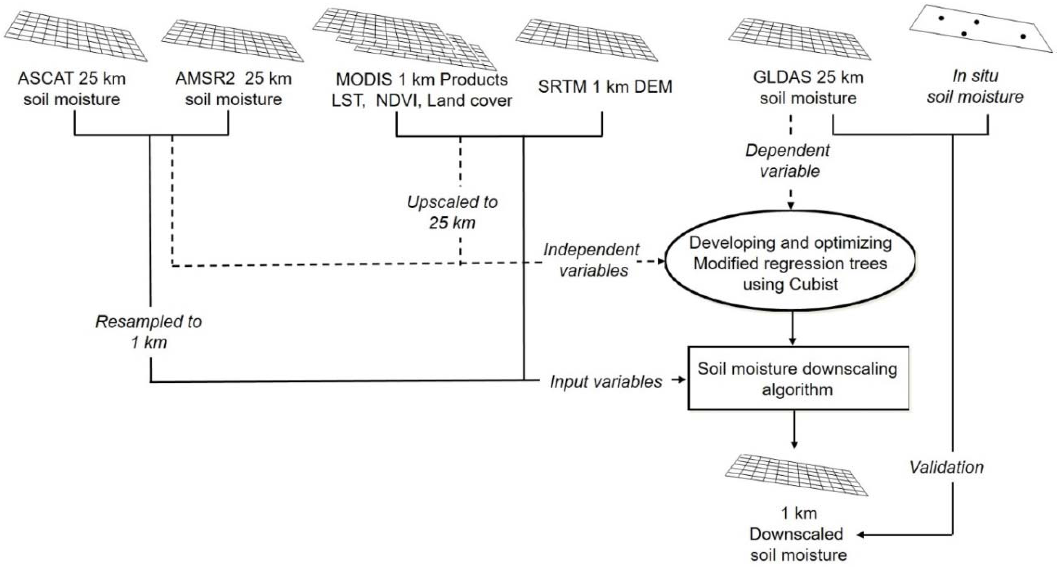
Figure 3.
Performance of modified regression trees with different numbers of rules to identify the optimum number of rules.
Figure 3.
Performance of modified regression trees with different numbers of rules to identify the optimum number of rules.

Figure 4.
Calibration (left) and validation (right) results of the soil moisture downscaling model proposed in this study.
Figure 4.
Calibration (left) and validation (right) results of the soil moisture downscaling model proposed in this study.

Figure 5.
Temporal pattern of GLDAS, downscaled, and in situ soil moisture data with precipitation information for each station (a–n) from May to September 2015.
Figure 5.
Temporal pattern of GLDAS, downscaled, and in situ soil moisture data with precipitation information for each station (a–n) from May to September 2015.
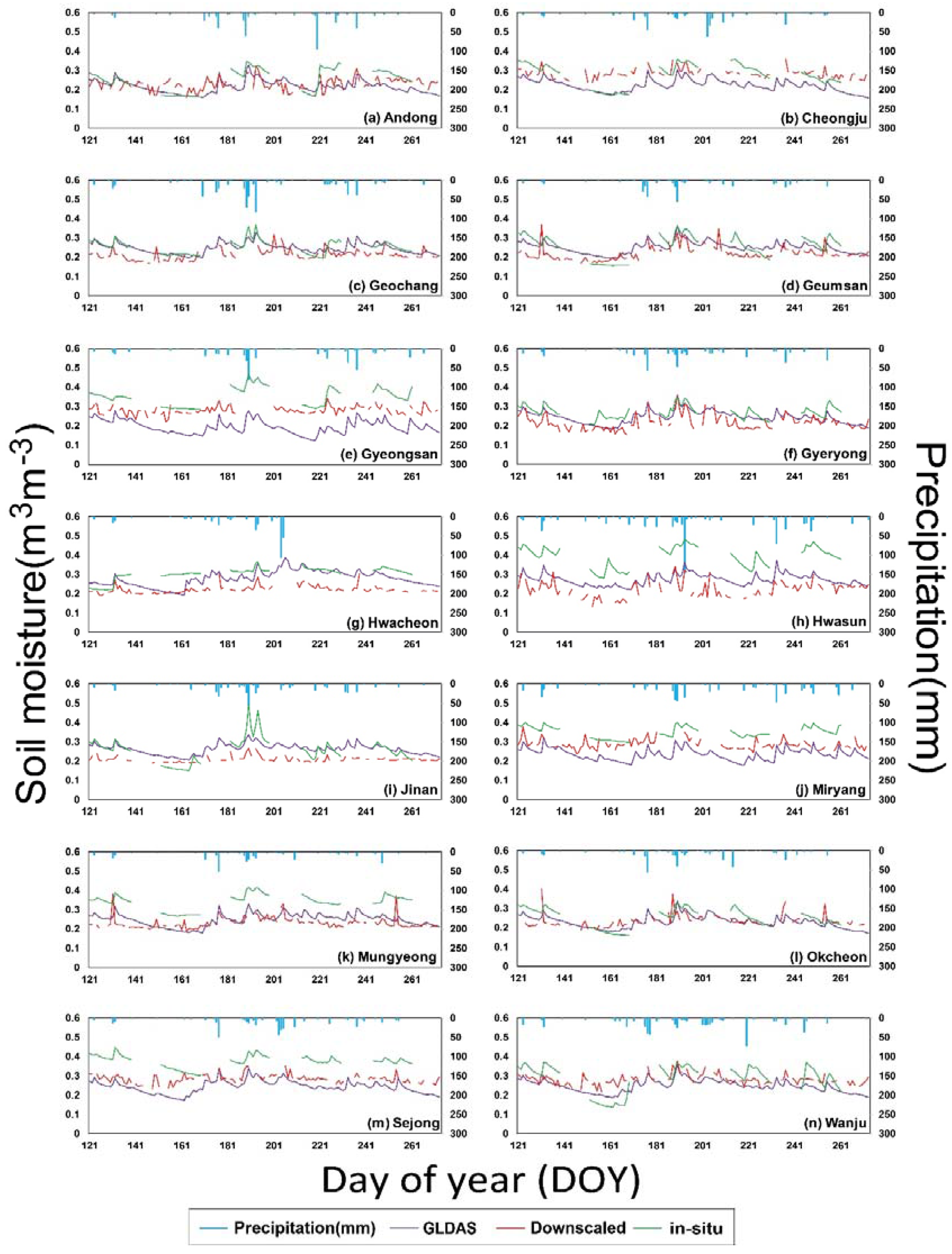
Figure 6.
Scatterplots between 1 km downscaled and in situ soil moisture data (p < 0.01) by station (a–n) in 2015.
Figure 6.
Scatterplots between 1 km downscaled and in situ soil moisture data (p < 0.01) by station (a–n) in 2015.

Figure 7.
Comparison of monthly spatial distribution between 1 km downscaled and GLDAS soil moisture data in 2015.
Figure 7.
Comparison of monthly spatial distribution between 1 km downscaled and GLDAS soil moisture data in 2015.

Figure 8.
Spatial distribution of (a) correlation coefficients, (b) RMSE, (c) p-values, and (d) rRMSE values between GLDAS and the 1 km downscaled soil moisture data during the growing season in 2015.
Figure 8.
Spatial distribution of (a) correlation coefficients, (b) RMSE, (c) p-values, and (d) rRMSE values between GLDAS and the 1 km downscaled soil moisture data during the growing season in 2015.

Figure 9.
Spatial distribution of the daily 1 km downscaled soil moisture and Tropical Rainfall Measuring Mission (TRMM) precipitation data around the Korean Peninsula from 10 to 16 July 2015.
Figure 9.
Spatial distribution of the daily 1 km downscaled soil moisture and Tropical Rainfall Measuring Mission (TRMM) precipitation data around the Korean Peninsula from 10 to 16 July 2015.
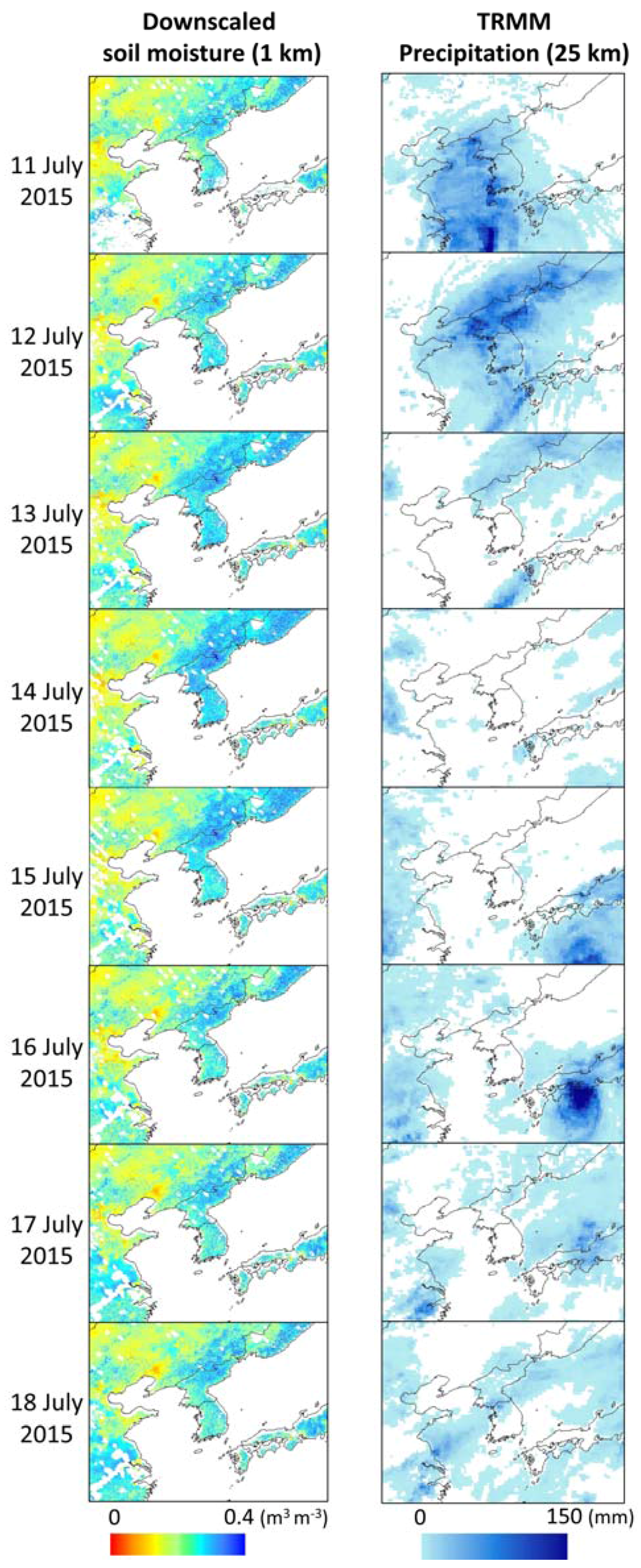
Table 1.
Summary of remote sensing-derived independent variables and Global Land Data Assimilation System (GLDAS) soil moisture (dependent variable) to develop a machine learning-based soil moisture downscaling model. Shuttle Radar Topography Mission (SRTM) data was released in 2013.
Table 1.
Summary of remote sensing-derived independent variables and Global Land Data Assimilation System (GLDAS) soil moisture (dependent variable) to develop a machine learning-based soil moisture downscaling model. Shuttle Radar Topography Mission (SRTM) data was released in 2013.
| Variable Type | Data | Product | Spatial Resolution | Temporal Resolution | Unit |
|---|---|---|---|---|---|
| Independent variables | AMSR2 | Soil moisture | 25 km | daily | % |
| ASCAT | 25 km | % | |||
| MODIS | Land Surface Temperature (LST) | 1 km | 8 days | K | |
| Normalized Difference Vegetation Index (NDVI) | 16 days | - | |||
| Land cover | 500 m | yearly | - | ||
| SRTM | Digital Elevation Model (DEM) | 90 m | - | m | |
| Dependent variable | GLDAS | Soil moisture | 25 km | daily | kg·m−2 |
Table 2.
Geographical and land cover characteristics of 14 ground stations in South Korea.
| Station | Latitude (° N) | Longitude (° E) | Altitude (m) | Land Cover (1 km) | Land Cover (25 km) | |
|---|---|---|---|---|---|---|
| a | Andong | 36.538 | 128.805 | 112 | Crop | Forest |
| b | Cheongju | 36.588 | 127.505 | 57 | Crop | Crop, Forest |
| c | Geochang | 35.678 | 127.923 | 195 | Crop | Forest, Crop |
| d | Geumsan | 36.126 | 127.496 | 167 | Crop | Forest |
| e | Gyeongsan | 35.817 | 128.813 | 57 | Crop | Crop, Built up |
| f | Gyeryong | 36.200 | 127.280 | 176 | Forest | Forest |
| g | Hwacheon | 38.114 | 127.708 | 176 | Crop | Forest |
| h | Hwasun | 34.970 | 127.070 | 162 | Crop | Forest |
| i | Jinan | 35.761 | 127.438 | 347 | Crop | Forest |
| j | Miryang | 35.447 | 128.757 | 53 | Crop | Crop, Forest |
| k | Mungyeong | 36.608 | 128.208 | 106 | Crop | Forest, Crop |
| l | Okcheon | 36.300 | 127.596 | 126 | Crop | Forest |
| m | Sejong | 36.563 | 127.298 | 22 | Crop | Crop, Built up |
| n | Wanju | 35.984 | 127.220 | 52 | Crop | Crop, Built up |
Table 3.
Six selected sub-models from the optimized regression tree-based downscaling model. Each sub-model consists of a rule and its associated multivariate regression model. The number of cases (i.e., samples) and the mean soil moisture corresponding to each rule are also presented.
Table 3.
Six selected sub-models from the optimized regression tree-based downscaling model. Each sub-model consists of a rule and its associated multivariate regression model. The number of cases (i.e., samples) and the mean soil moisture corresponding to each rule are also presented.
| Rule 1: [7139 cases, mean 0.13 m3·m−3] if DEM > 253, Land cover in barren, LST > 270.07, then GLDAS = 0.3293702 + 0.115NDVI + 1.6 × 10⁻⁵DEM − 0.00083LST + 0.16AMSR2 − 0.039 ASCAT Rule 2: [2557 cases, mean 0.14 m3·m−3] if ASCAT ≤ 0.1713, DEM ≤ 2851, Land cover in grassland, LST > 270.07, then GLDAS = 0.5576747 − 0.00154LST + 2.4 × 10⁻⁵DEM − 0.041ASCAT + 0.14AMSR2 + 0.02NDVI Rule 3: [1926 cases, mean 0.16 m3·m−3] if ASCAT > 0.1713, Land cover in grassland, LST > 270.07, NDVI > 0.0493, then GLDAS = 0.573495 − 0.00156LST + 0.082ASCAT + 0.048NDVI + 0.08AMSR2 + 2.3 × 10⁻⁶DEM Rule 40: [1800 cases, mean 0.29 m3·m−3] if DEM > 591, Land cover in forest, shrublands, savannas, cropland, 271.43 < LST ≤ 276.99, NDVI > 0.14222, then GLDAS = −0.2904213 + 0.239NDVI − 0.66AMSR2 + 0.00191LST − 1.0 × 10⁻⁵DEM Rule 45: [1426 cases, mean 0.21 m3·m−3] if AMSR2 > 0.0471, 108 < DEM ≤ 115, then GLDAS = 2.4442403 − 0.0139204DEM − 0.00231LST + 0.117ASCAT − 0.078NDVI + 0.08AMSR2 Rule 58: [2123 cases, mean 0.16 m3·m−3] if ASCAT ≤ 0.225824, Land cover in forest, shrublands, savannas, LST ≤ 271.43, NDVI ≤ −0.015709, then GLDAS = 0.2094862 − 0.701NDVI − 0.218ASCAT + 0.33AMSR2 + 0.00047LST + 1.4 × 10⁻⁶DEM |
Table 4.
The usage in percentage of input variables in the rules and multi-variate regression models produced from the optimized regression trees.
Table 4.
The usage in percentage of input variables in the rules and multi-variate regression models produced from the optimized regression trees.
| Variables | Attribute Usage | |
|---|---|---|
| Rules | Regression Models | |
| Land cover | 91% | - |
| DEM | 83% | 97% |
| LST | 82% | 98% |
| NDVI | 61% | 91% |
| ASCAT | 42% | 84% |
| AMSR2 | 8% | 74% |
© 2017 by the authors. Licensee MDPI, Basel, Switzerland. This article is an open access article distributed under the terms and conditions of the Creative Commons Attribution (CC BY) license (http://creativecommons.org/licenses/by/4.0/).
Share and Cite
MDPI and ACS Style
Park, S.; Park, S.; Im, J.; Rhee, J.; Shin, J.; Park, J.D. Downscaling GLDAS Soil Moisture Data in East Asia through Fusion of Multi-Sensors by Optimizing Modified Regression Trees. Water 2017, 9, 332. https://doi.org/10.3390/w9050332
AMA Style
Park S, Park S, Im J, Rhee J, Shin J, Park JD. Downscaling GLDAS Soil Moisture Data in East Asia through Fusion of Multi-Sensors by Optimizing Modified Regression Trees. Water. 2017; 9(5):332. https://doi.org/10.3390/w9050332
Chicago/Turabian StylePark, Seonyoung, Sumin Park, Jungho Im, Jinyoung Rhee, Jinho Shin, and Jun Dong Park. 2017. "Downscaling GLDAS Soil Moisture Data in East Asia through Fusion of Multi-Sensors by Optimizing Modified Regression Trees" Water 9, no. 5: 332. https://doi.org/10.3390/w9050332
Note that from the first issue of 2016, this journal uses article numbers instead of page numbers. See further details here.