Uncertainty of Hydrological Drought Characteristics with Copula Functions and Probability Distributions: A Case Study of Weihe River, China

Abstract

This study investigates the sensitivity and uncertainty of hydrological droughts frequencies and severity in the Weihe Basin, China during 1960–2012, by using six commonly used univariate probability distributions and three Archimedean copulas to fit the marginal and joint distributions of drought characteristics. The Anderson-Darling method is used for testing the goodness-of-fit of the univariate model, and the Akaike information criterion (AIC) is applied to select the best distribution and copula functions. The results demonstrate that there is a very strong correlation between drought duration and drought severity in three stations. The drought return period varies depending on the selected marginal distributions and copula functions and, with an increase of the return period, the differences become larger. In addition, the estimated return periods (both co-occurrence and joint) from the best-fitted copulas are the closet to those from empirical distribution. Therefore, it is critical to select the appropriate marginal distribution and copula function to model the hydrological drought frequency and severity. The results of this study can not only help drought investigation to select a suitable probability distribution and copulas function, but are also useful for regional water resource management. However, a few limitations remain in this study, such as the assumption of stationary of runoff series.

1. Introduction

Hydrological drought refers to a lack of water in the hydrological system and gives rise to negative impacts on river ecosystems and human lives [1]. Hydrological droughts are typically defined as periods when streamflow below a pre-defined threshold, called the threshold level method (TLM) [2]. Advantages of the TLM are (i) no a priori knowledge of probability distributions is required, and (ii) it directly produces drought characteristics (e.g., duration, severity, frequency). When the variable of interest ($\mathrm{x}$) (i.e., soil moisture, groundwater storage, or discharge) is below a predefined threshold ($\tau$), a drought is assumed to have occurred. A constant or a threshold can be used, and because a variable threshold level takes seasonal patterns into account, it has been widely used [3,4]. The threshold is usually assumed to be equal to a given percentile of the flow duration curve between the 30 percentile flow ($Q_{30}$) and the 5percentile flow ($Q_5$) [5], or the threshold can be obtained by fitting some kind of statistical function through the data (normal, gamma, beta, etc.) [6]. The threshold is 25percentile ($Q_{25}$), meaning that a drought occurs when the streamflow is below the 25th percentile flow from the duration curve. The number of drought events obtained from the $Q_{30}$, $Q_{25}$, $Q_{20}$, $Q_{15}$, $Q_{10}$, and $Q_5$ were compared with a previous study [7]. Based on the yearbook of “the drought history in China (1949–2000)”, which reported that the main drought years in the Weihe River are 1962, 1969, 1971–1972, 1977, 1982, 1986, 1994, 1995, and 1997, drought events defined by $Q_{25}$ are the closest to the historical drought conditions. Therefore, the threshold level in this study selected $Q_{25}$ to define drought events and examine hydrological drought characteristics in the Weihe River Basin.

Since hydrological droughts are complex events, one index cannot provide a comprehensive evaluation. A bivariate distribution is derived for describing the correlated hydrology drought characteristic variables. For instance, bivariate normal distribution [8], bivariate exponential distribution [9], and bivariate gamma distribution [10] are often applied to study flood problems. However, because the hydrology drought characteristic variables are highly correlated and may obey different marginal distribution functions, one of the drawbacks for these bivariate distributions is that the same family is needed for each marginal distribution [11].

Copulas are functions that join univariate distribution functions to form multivariate distribution functions [12]. Sklar [13] introduced copulas, and they have been used in insurance and finance [14]. Because of the flexibility of copulas, they became popular in hydrological analysis [15]. Especially, Archimedean copulas, such as Clayton, Frank, and Gumbel-Hougard copulas, are the most popular family used in hydrology [16] and have been widely applied to model the dependence between hydrological variables [17]. When using copula functions analysis of hydrological droughts, several marginal distribution functions have been commonly used to fit drought duration and drought severity, such as exponential (EXP), gamma (GAMA), lognormal (LOGN), general Pareto (GP), generalized extreme value (GEV), and Weibull (WBL) [18] distributions. The inversion of Kendall’s method was usually used to estimate the copula parameter [19], and the goodness of fit was usually tested by the least root mean square error (RMES), Kolmogorov-Smirnov (KS) test, Anderson-Darling (AD) test, Akaike information criterion (AIC), ordinary least squares (OLS), and Bayesian information criterion (BIC) [20].

However, the selection of a threshold directly influences the duration and severity of drought events, and it is an uncertainty factor in modeling the bivariate distribution of hydrological droughts. Due to the changing environment and the impact from human activities, the variability of hydrological drought properties is also an important uncertainty factor. Since there are some goodness of fit test methods for choosing appropriate margin probability distributions and copula functions, the final selections may be different depending on the different candidate margins distributions and copulas. Therefore, it is necessary to investigate the uncertainty and sensitivity in modeling the joint distribution of hydrological droughts. In this paper, we choose six commonly-used univariate probability distributions as the candidate margins for drought duration and severity, and three Archimedean copulas are employed to match the joint distributions.

The remaining parts of this paper are organized as follows: Section 2 introduces the case study and the data from three hydrometric stations, the methodologies for defining the hydrological drought, six univariate models, and the theory of copulas and the formula of the return period; Section 3 shows the primary results, including the univariate and bivariate drought frequency analysis and the calculation of return periods; Section 4 discusses the sensitive and uncertainty of drought frequency analysis.; and, finally, the main conclusions are given in Section 5.

2. Materials and Methods

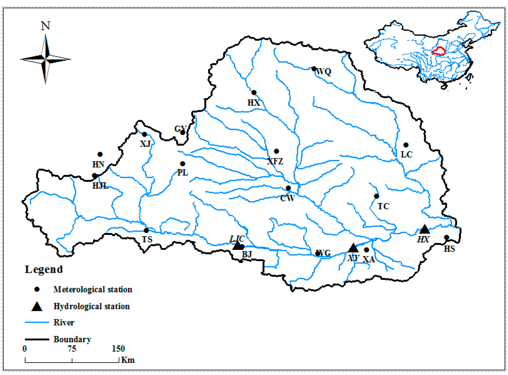
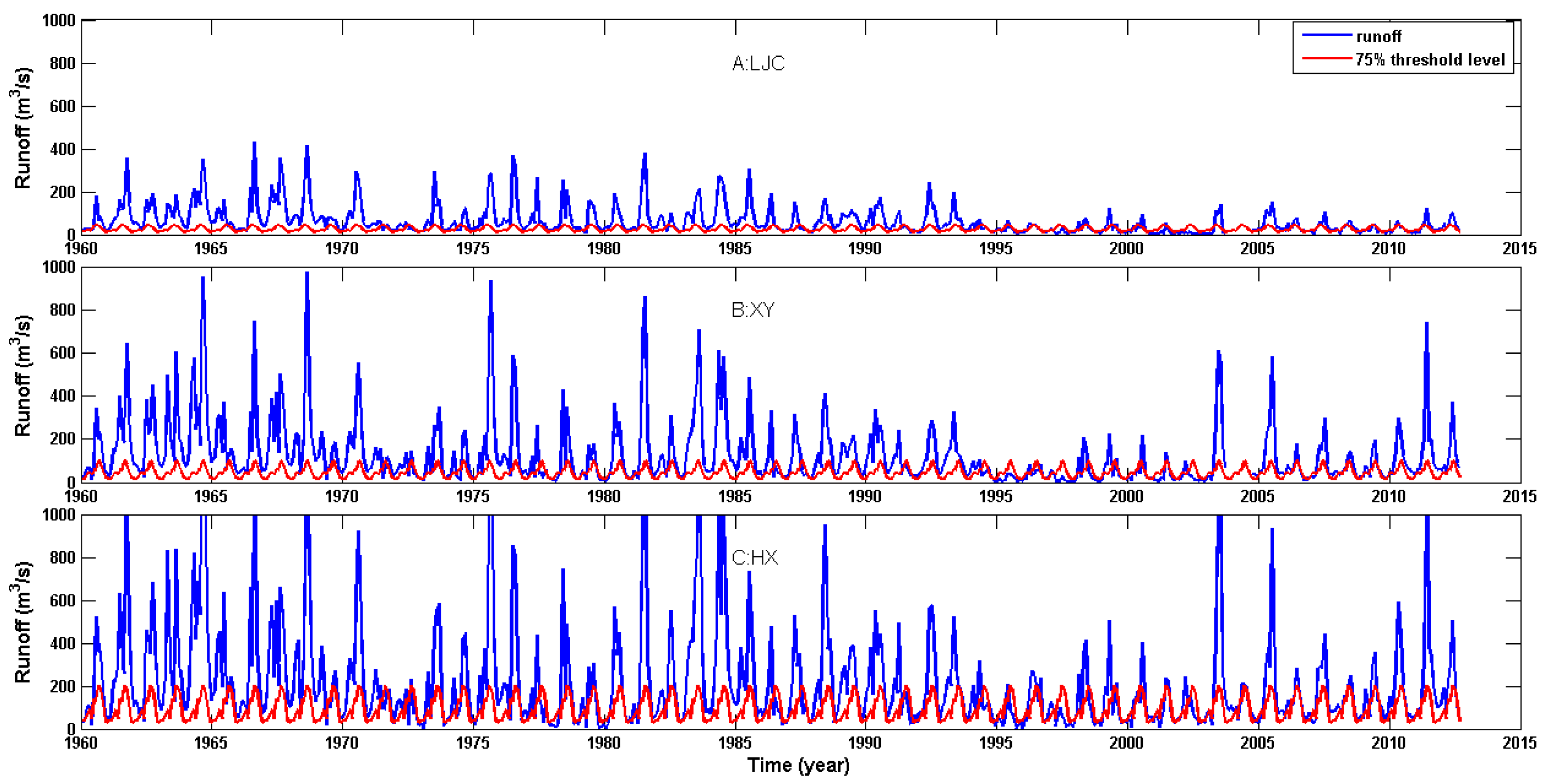
2.1. Weihe River Basin and Data

The Weihe River Basin, with a drainage area of 134,800 km², is the largest tributary of the Yellow River in North China (Figure 1) (between 104°–110° E and 34°–38° N). This basin originates from the north of Niaoshu Mountain with an altitude of 3485 m above sea level. The most important topographic feature of the Weihe River Basin is the Loess Plateau in the north, which is the main source of sediments in the river [21]. The annual average temperature ranges between 9.3 °C and 14.4 °C, the annual mean precipitation amounts are in the range of 558–750 mm with a general increasing trend from north to south, and the annual mean runoff amounts are 10.37 billion m³. The runoff from July to September accounts for about 60–70% of the annual discharge [22]. Agricultural losses due to local drought disasters occupy over 50% of the total losses [23].

The hydrological stations of Linjiacun (LJC), Xianyang (XY) and Huaxian (HX) are located in the upper, middle, and lower streams for the main river channel (Figure 1).

The data of three stations are provided by the Institute of Soil and Water Conservation (http://loess.geodata.cn/), Chinese Academy of Sciences and Ministry of Water Resources. The monthly streamflow covers the period between 1960 and 2012 years. Linjiacun and Xianyang station lack data in 2004.

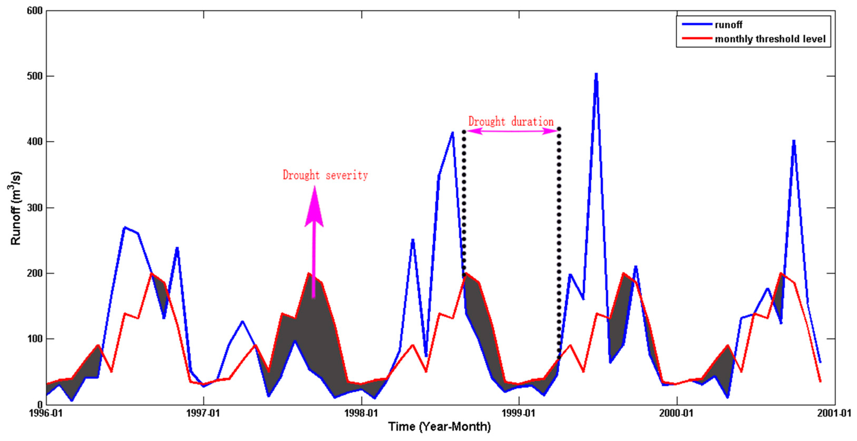
2.2. Defining Drought Duration and Severity

A drought event starts when the variable ($x$) is below the threshold level (onset; $t=1$) and the event continues until the threshold is exceeded again (recovery; $t=T$). Each drought event ($i$) can be characterized by its duration and by some measure of the severity of the event (Figure 2).

The duration of a drought event is calculated by [24]:

$$\delta \left(t\right)=\{\begin{array}{l}1\hspace{1em}\mathrm{if}\hspace{0.17em}x\left(t\right)<\tau \left(t\right)\\ 0\hspace{1em}\mathrm{if}\hspace{0.17em}x\left(t\right)\ge \tau \left(t\right)\end{array}$$

(1)

$$D_i={\displaystyle \sum _{t=1}^T\delta \left(t\right)}·\mathrm{\Delta }t$$

(2)

where $\delta \left(t\right)$ is a binary variable indicating a drought situation with respect to time $t$, x(t) is the hydrological variable on time $t$, $\tau \left(t\right)$ is the threshold level of that hydrological variable with respect to time $t$, $D_i$ is the duration of drought event $i$, and $\mathrm{\Delta }t$ is the time step of $t$.

For fluxes the most commonly-used severity measure is the deficit volume, calculated; by summing up the differences between the actual flux and the threshold level over the drought period [25]. The equation is:

$$s\left(t\right)=\{\begin{array}{l}\tau \left(t\right)-x\left(t\right)\hspace{1em}\mathrm{if}\hspace{0.17em}x\left(t\right)<\tau \left(t\right)\\ 0\hspace{1em}\hspace{1em}\hspace{1em}\hspace{1em}\hspace{1em}\mathrm{if}\hspace{0.17em}x\left(t\right)\ge \tau \left(t\right)\end{array}$$

(3)

$$S_i={\displaystyle \sum _{t=1}^{T}s\left(t\right)}·\mathrm{\Delta }t$$

(4)

where $s\left(t\right)$ is the deviation with respect to time $t$, and $S_i$ is the deficit of drought event $i$.

The streamflow (m³/s) is converted into runoff depth (mm) by:

$$R=\frac{Q\times t}{1000\times A}$$

(5)

where $R$ is the runoff depth in mm; $Q$ is the streamflow in m³/s, $t$ is the monthly time in seconds, and $A$ is the drainage area in km².

2.3. Marginal Distribution Model and Copula-Based Models

Six commonly-used univariate probability distributions are selected as the candidate margins for drought duration and drought severity. They are the exponential (EXP), gamma (GAM), log-normal (LOGN), generalized Pareto (GP), generalized extreme value (GEV), and Weibull (WBL) distributions. The cumulative distribution functions (CDF) of six univariate distributions are given in

Table 1. Univariate cumulative distribution functions.

Distribution	CDF	Parameters
Exponential (EXP)	$F\left(x\right)=1-e^{-x/\mu }$	$\mu$: scale
Gamma (GAM)	$F\left(x\right)=\frac{{\beta }^{-\alpha }}{\mathrm{\Gamma }\left(\alpha \right)}{\displaystyle {\int }_0^x{t}^{\alpha -1}{e}^{-t/\beta }dt}$	$\alpha$: shape
		$\beta$: scale
Log-normal (LOGN)	$F\left(x\right)=\frac{1}{\sigma \sqrt{2\pi }}{\displaystyle {\int }_0^x\frac{e-{\left(\ln \left(t\right)-\mu \right)}^2/2{\sigma }^2}{t}dt}$	$\mu$: mean
		$\sigma$: standard deviation
Generalized Pareto (GP)	$F\left(x\right)=1-\exp \left({\kappa }^{-1}\ln \left(1-\frac{\kappa \left(x-\xi \right)}{\alpha }\right)\right)$	$\kappa$: shape
		$\alpha$: scale
		$\xi$: location
Generalized extreme value (GEV)	$F\left(x\right)=\exp \left(-\exp \left({\kappa }^{-1}\ln \left(1-\frac{\kappa \left(x-\xi \right)}{\alpha }\right)\right)\right)$	$\kappa$: shape
		$\alpha$: scale
		$\xi$: location
Weibull (WBL)	$F\left(x\right)=1-e^{-{\left(x/a\right)}^b}{\mathrm{{\rm I}}}_{\left(0,\infty \right)}\left(x\right)$	$a$: scale
		$b$: shape

. The maximum likelihood method is used to estimate the parameters. Akaike information criterion (AIC) [26] and the Anderson Darling (AD) [27] test are used to select the best univariate distribution.

Developed by Sklar [13], copulas are functions that link univariate distribution functions to form multivariate distribution functions, in which the domain is [0, 1]. In terms of two random variables, Sklar’s theorem, states that if $F_{X,Y}\left(x,y\right)$ is a two-dimensional joint cumulative distribution function, $F_X\left(x\right)$ and $F_Y\left(y\right)$ are marginal distribution functions of variables $X$, $Y$, then there exists a copula $C$ such that:

$$F_{X,Y}\left(x,y\right)=C\left(F_X\left(x\right),F_Y\left(y\right)\right)$$

(6)

In which $c$ is the density function of $C$, defined as:

$$c\left(u,v\right)=\frac{{\partial }^{2}C\left(u,v\right)}{\partial u\partial v}$$

(7)

In this study, we choose widely-used three mono-parameter Archimedean copulas (Clayton, Frank, and Gumbel-Hougard) as the candidates for modeling the joint distribution of hydrological drought properties. Three copulas are defined as shown in

Table 2. Copula functions.

Copulas	CDF	Parameters
Clayton	$C\left(u,v\right)={\left(u^{-\theta }+v^{-\theta }-1\right)}^{-\frac{1}{\theta }}$	$\theta \ge 0$
Frank	$C\left(u,v\right)=-\frac{1}{\theta }\ln \left[1+\left(\frac{\left(e^{-\theta u}-1\right)\left(e^{-\theta v}-1\right)}{e^{-\theta }-1}\right)\right]$	$\theta \ne 0$
Gumel	$C\left(u,v\right)=\exp \left\{-{\left[{\left(-\ln u\right)}^{\theta }+{\left(-\ln v\right)}^{\theta }\right]}^{\frac{1}{2}}\right\}$	$\theta \ge 1$

. The inference function for margins (IFM), suggested by Joe [28], is employed to estimate the parameter in copulas. The ordinary least squares (OLS) and Akaike information criterion (AIC) are used for testing the goodness of fit.

2.4. Return Period of Droughts

The return period of a variable, defined as the average elapsed time between occurrences of an event with a certain magnitude, or greater [29]. In this study, the return period of droughts can be defined by drought duration or drought severity as [30]:

$$T_D=\frac{N}{n\left(1-F_D\left(d\right)\right)}$$

(8)

$$T_S=\frac{N}{n\left(1-F_S\left(s\right)\right)}$$

(9)

where $T_D$ is the return period of drought duration, $T_S$ is the return period of drought severity; $N$ is the length of data series; $n$ is the numbers of drought events, and $F_D(d)$ and $F_S\left(s\right)$ are cumulative distribution function of drought duration and severity, respectively

There are two cases of bivariate return periods; one is the drought duration exceeding a specific value and the drought severity exceeding another specific value ($D\ge d\hspace{0.17em}\mathrm{and}\hspace{0.17em}S\ge s$), called co-occurrence return period ($T_0$). Another case is the drought duration exceeding a specific value or the drought severity exceeding another specific value ($D\ge d\hspace{0.17em}\mathrm{or}\hspace{0.17em}S\ge s$), called the joint return period ($T_{\alpha }$). Both return periods, in terms of the copula-based bivariate drought distribution, are described below [31]:

$$T_0=\frac{N}{nP\left(D\ge d\cap S\ge s\right)}=\frac{N}{n\left(1-F_D\left(d\right)-F_S\left(s\right)+F_{DS}\left(d,s\right)\right)}=\frac{N}{n\left(1-F_D\left(d\right)-F_S\left(s\right)+C\left(F_D\left(d\right),F_S\left(s\right)\right)\right)}$$

(10)

$$T_{\alpha }=\frac{N}{nP\left(D\ge d\cup S\ge s\right)}=\frac{N}{n\left(1-F_{DS}\left(d,s\right)\right)}=\frac{N}{n\left(1-C\left(F_D\left(d\right),F_S\left(s\right)\right)\right)}$$

(11)

3. Results

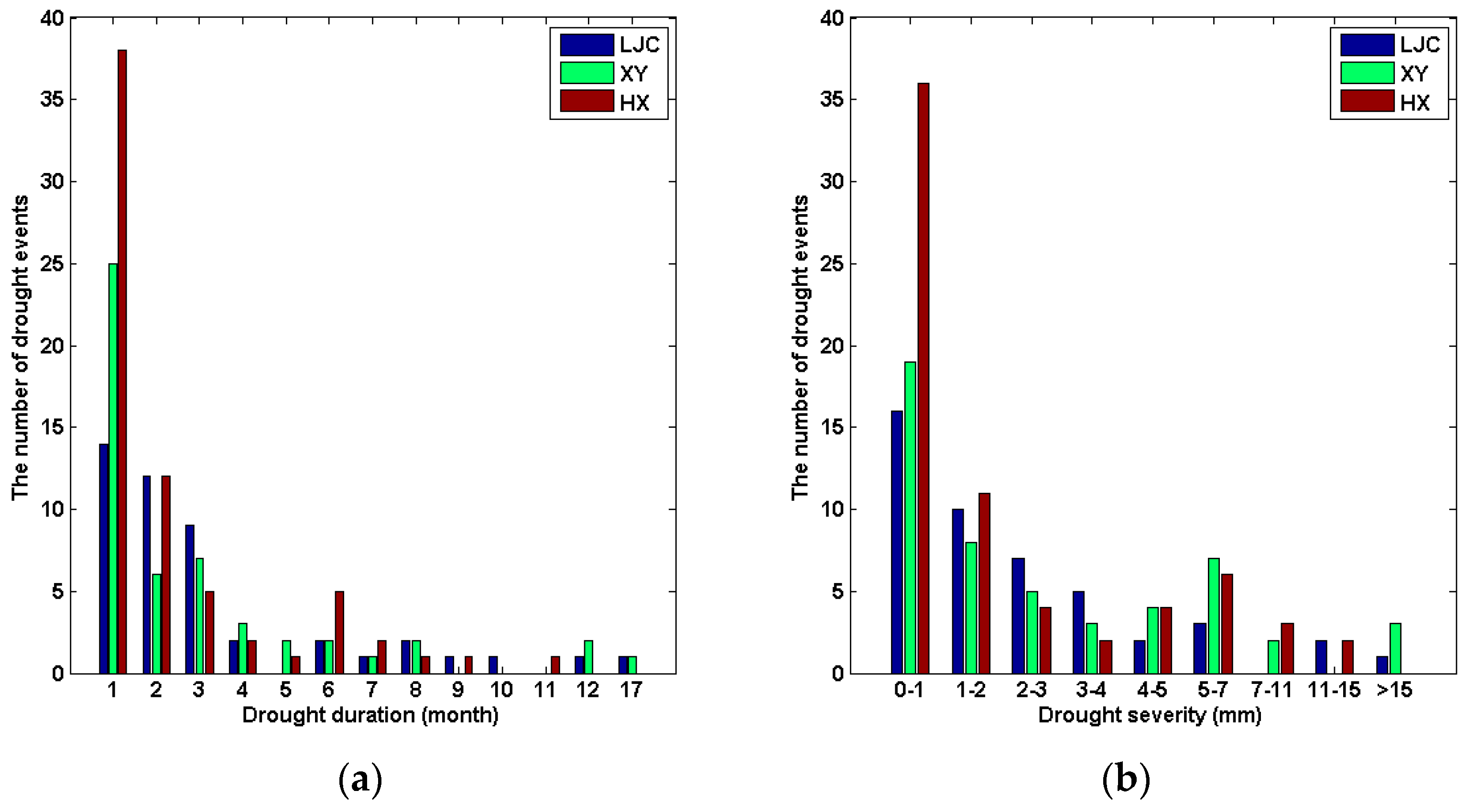
3.1. Drought Duration and Severity Characteristics

Based on the $Q_{25}$ threshold level of monthly runoff, there are a total of 46, 51, and 68 drought events, respectively, in three stations (Linjiacun, Xianyang, Huaxian) during 1960–2012 (Figure 3). Figure 4 shows the number of drought events of different drought duration and severity at three stations. The main statistical characteristic values of drought duration and drought severity are listed in

Table 3. Hydrological drought index of single-feature statistical characteristic values.

		Mean	Std.dev.	Max	Min	Cv	SK
Drought duration (month)	LJC	3.391	3.363	17	1	0.992	2.172
	XY	3.059	3.343	17	1	1.093	2.316
	HX	2.382	2.273	11	1	0.954	1.879
Drought Severity (mm)	LJC	3.009	5.081	30.436	0.019	1.689	3.964
	XY	3.726	5.387	23.946	0.002	1.446	2.513
	HX	2.175	2.959	15.169	0.001	1.360	2.074

Note: “Std.dev” indicates standard deviation. “Cv” indicates the coefficient of variation, and “SK” indicates skewness coefficient. LJC indicates Linjiacun station, XY indicates Xianyang station, HX indicates Huaxian station.

. The most severe drought lasted for 17 months in Linjiacun and Xianyang stations. The average drought durations are 3.391, 3.059, and 2.382 months, respectively, at the three stations. This is why the number of drought events of LJC station (46) and XY station (51) are less than those of HX station (68). The skewness coefficient (which is a measure of the asymmetry of the probability distribution of a real-valued random variable about its mean) of drought severity is also larger than the drought duration. In view of the drought duration, the dispersion degree of Linjiacun station is the smallest. In view of the drought severity, the dispersion degree of Xianyang station is the smallest.

The relationship between drought duration and drought severity is very good (

Table 4. Correlation between the hydrological drought characteristics’ indices.

Correlation Coefficient	LJC ($\mathit{D}~\mathit{S}$)	XY ($\mathit{D}~\mathit{S}$)	HX ($\mathit{D}~\mathit{S}$)
$\rho$	0.883	0.916	0.885
$\tau$	0.705	0.644	0.639
${\rho }_s$	0.827	0.803	0.776

Note: $\rho$ indicates the Pearson linearly-dependent coefficient, $\tau$ indicates the Kendall rank correlation coefficient; ${\rho }_s$ indicates the Spearman rank correlation coefficient.

); they reflect that there is very strong correlation between drought duration and drought severity in three stations. The Pearson linearly-dependent coefficients in the three stations are over 0.88. The Spearman rank correlation coefficient exceeded 0.77. For the Kendall rank correlation coefficient, its surpass 0.63. For example, the Pearson linearly-dependent coefficient $\rho$ is 0.883, 0.916, and 0.885, respectively, in the three stations, which suggests the importance of using copulas based on the drought frequency analysis method.

3.2. Marginal Distributions and Copula Functions

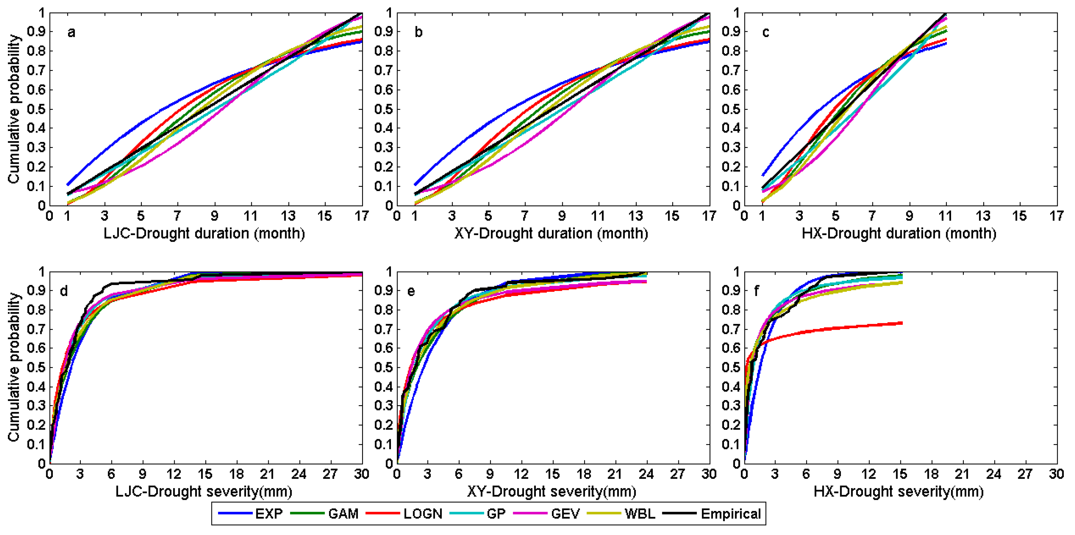
3.2.1. Selected Marginal Distributions

Table 5. The estimated parameters by the maximum likelihood method.

Margin		Parameter	LJC	XY	HX
Duration	EXP	$\mu$	3.391	3.059	2.382
	GAM	$\alpha$	1.612	1.399	1.743
		$\beta$	2.103	2.186	1.366
	LOGN	$\mu$	0.880	0.720	0.555
		$\sigma$	0.789	0.838	0.731
	GP	$\kappa$	−0.017	0.072	−0.056
		$\alpha$	3.449	2.838	2.515
	GEV	$\kappa$	5.062	3.783	4.958
		$\alpha$	0.330	0.011	0.159
		$\xi$	1.065	1.003	1.032
	WBL	$a$	3.637	3.197	2.580
		$b$	1.196	1.105	1.234
Severity	EXP	$\mu$	35.600	67.316	89.357
	GAM	$\alpha$	0.691	0.594	0.287
		$\beta$	51.513	113.247	311.259
	LOGN	$\mu$	2.696	3.169	2.073
		$\sigma$	1.510	1.805	7.138
	GP	$\kappa$	0.381	0.529	0.747
		$\alpha$	21.939	36.178	38.080
	GEV	$\kappa$	0.706	1.042	1.239
		$\alpha$	12.958	21.278	25.334
		$\xi$	11.151	15.605	16.587
	WBL	$a$	29.791	53.411	51.179
		$b$	0.768	0.706	0.417

lists the estimated parameters for six theoretical distribution models, and the results of AIC and AD test at the 99% ($\alpha =0.01$) significant level have shown in

Table 6. The goodness of fit of the marginal distribution.

		LJC		XY		HX
		AIC	AD	AIC	AD	AIC	AD
			p-Value		p-Value		p-Value
Duration	EXP	−76.856	0.243	−76.856	0.243	−39.335	0.393
	GAM	−98.198	0.945	−98.198	0.945	−50.448	0.962
	LOGN	−88.137	0.635	−88.137	0.635	−46.052	0.857
	GP	−90.31	0.000	−90.31	0.000	−52.657	0.000
	GEV	−93.289	0.873	−93.289	0.873	−53.595	0.982
	WBL	−100.749	0.975	−100.749	0.975	−59.937	0.986
Severity	EXP	−207.934	0.0295	−230.471	0.021	−307.066	0.0068
	GAM	−263.939	0.3543	−291.92	0.3002	−425.32	0.479
	LOGN	−232.344	0.1144	−256.857	0.0866	−339.99	0.0348
	GP	−427.811	0	−475.892	0	−676.391	0
	GEV	−282.934	0.6941	−312.324	0.4499	−386.761	0.174
	WBL	−281.932	0.5106	−315.351	0.6396	−415.183	0.2938

. According to AIC and the AD test, the best fitted marginal distributions are WBL and GEV, WBL and WBL, and WBL and GAM, at the three stations, for drought duration and severity, respectively. Even though the GP model has relatively low AIC, the existence of “outliers” resulting in the GP distribution is not acceptable by the AD test for drought duration and drought severity, the EXP model is also not acceptable by the AD test for the fit of drought severity at Huaxin station. Figure 5 compares the six fitted distributions with empirical distributions of the identified drought characteristic variables in the three stations. The estimated theoretical cumulative probabilities for the best-fitting distribution are quite close to the empirical ones, which denotes that these probability distributions perform fairly well. Due to the existence of a few very small value (drought severity are 0.000761 mm, 0.03164 mm, 0.04114 mm, and 0.082 mm, respectively) of drought severity at HX station, the cumulative distribution function of LOGN only goes up to 0.7.

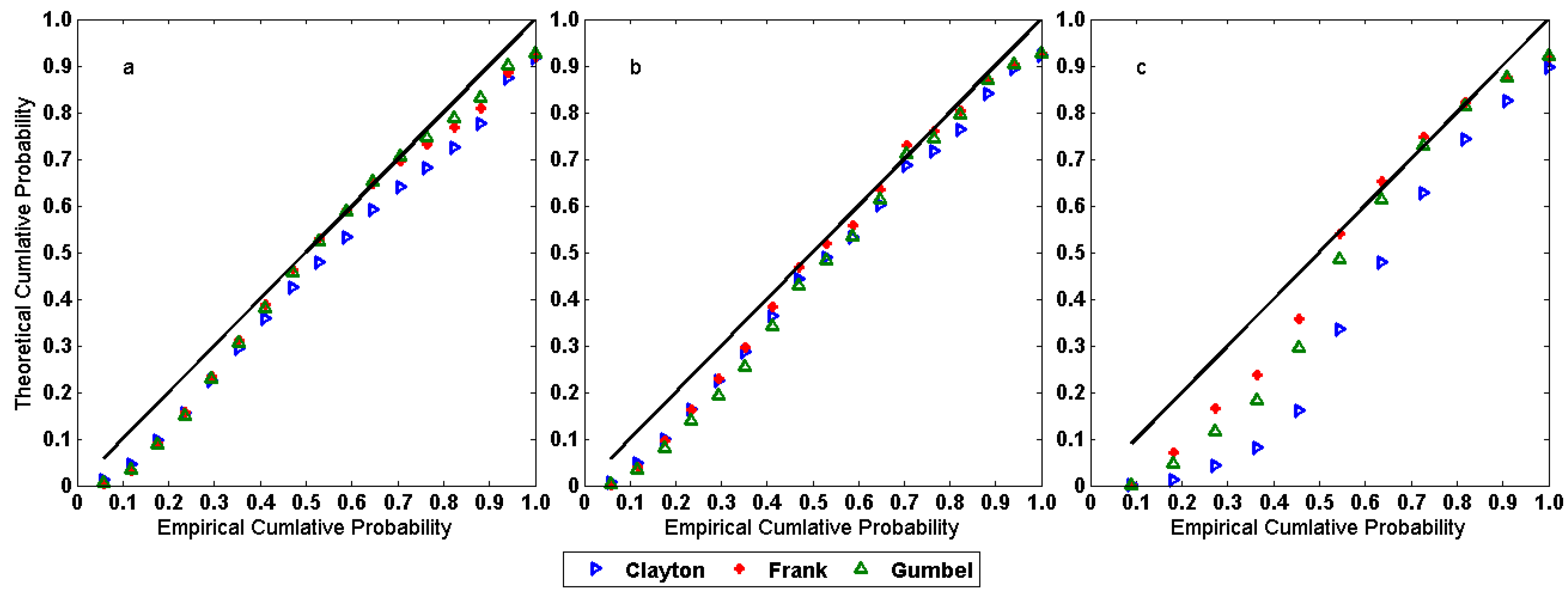
3.2.2. Selected Copula Functions

The results of the parameters and goodness of fit of the candidate bivariate copula functions are shown in

Table 7. Parameters and the goodness of fit of the bivariate distributions based on copulas.

Copula	Parameters and Goodness of Fit Index	LJC	XY	HX
Clayton	$\theta$	2.098	7.132	0.050
	OLS	0.071	0.057	0.181
	AIC	−86.783	−94.304	−34.542
Frank	$\theta$	9.829	40.229	28.017
	OLS	0.054	0.047	0.077
	AIC	−96.422	−100.643	−53.330
Gumbel	$\theta$	2.887	4.299	2.687
	OLS	0.050	0.063	0.104
	AIC	−98.522	−90.740	−46.728
Best Function		Gumbel	Frank	Frank

. According to OLS and AIC, the Frank copula is found to be the best-fitted one for Xianyang and Huaxian stations, and the Gumbel copula is the best-fitted for Linjiacun station. Figure 6 shows the probability-probability (PP) plot. It turns out that the estimated cumulative probabilities agree well with the empirical ones.

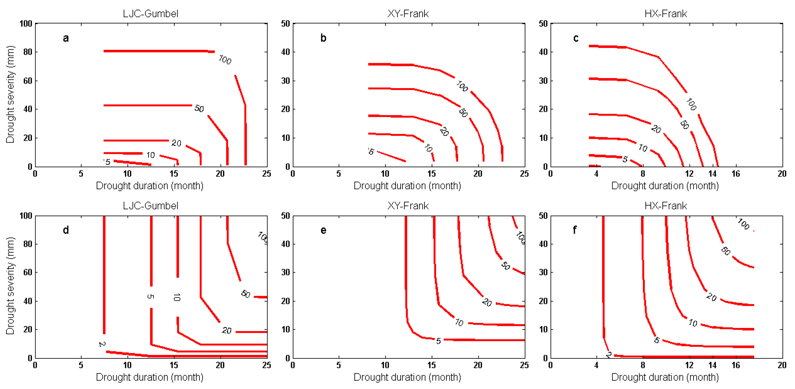
3.3. Return Period of Droughts

According to Equations (8) and (9), return periods of 2, 5, 10, 20, 50, and 100 years, defined by separate drought duration and drought severity, are summarized in

Table 8. Return periods defined by drought duration and severity in three stations.

		Drought Duration (month)			Drought Severity (mm)
		LJC	XY	HX	LJC	XY	HX
Return period (year)	2	7.452	8.152	6.551	1.156	1.690	1.041
	5	12.500	12.962	9.272	3.449	5.702	4.357
	10	15.370	15.759	10.903	6.327	9.520	7.711
	20	17.841	18.184	12.329	10.954	13.859	11.483
	50	20.718	21.021	14.001	21.752	20.269	16.877
	100	22.685	22.966	15.149	36.024	25.564	21.168

. For drought duration, the return period at Xianyag station is the largest, however, for drought severity, the return period of larger than 20 years for duration and severity at Linjiacun station is the largest. Considering two parameters, using joint probability distributions and copulas to calculate the co-occurrence return period and joint return period (in Figure 7), it is clear that the co-occurrence return period is greater than both of the return periods defined by the drought duration and drought severity separately, while the joint return period is less than both of the return periods. Under the same increasing range in univariate models, the increasing range of the co-occurrence return period is larger than the joint return period. This shows that these two kinds of combination return periods can be regarded as two extreme conditions of marginal distribution return periods. It is possible to estimate the interval of the actual return period according to the co-occurrence return period and the joint return period.

4. Sensitivity and Uncertainty of the Drought Frequency

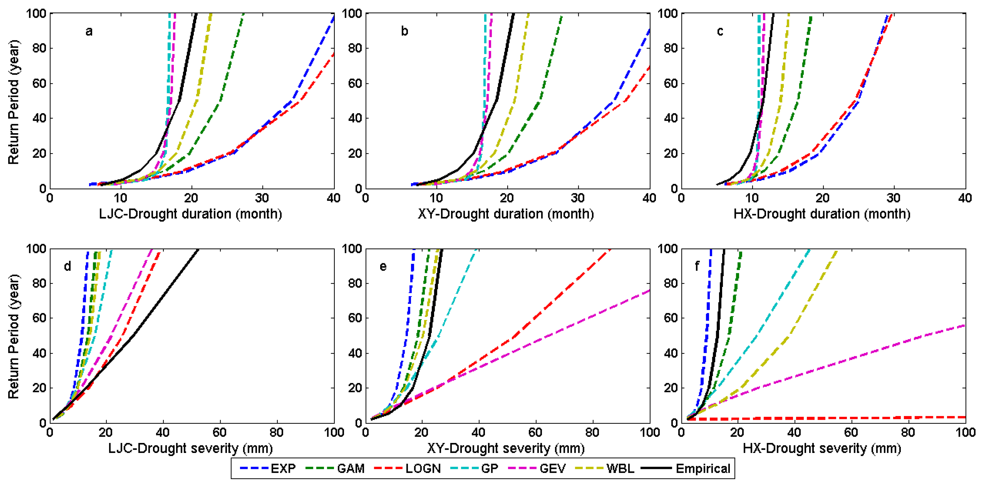
4.1. Effects of the Selection of Margin Distributions to the Return Period

The significance level of 99% ($\alpha =0.01$) is used to determine where the marginal distribution is to be rejected or accepted based on the AD test. The return periods of drought duration and severity are calculated based on six marginal distributions at three stations. Figure 8 shows their variability compared with the empirical return period. There are significant differences in the return period based on different marginal distributions. Considering drought duration, the return period of GP, GEV, and WBL models are best-fitted to the empirical value, the GEV and WBL models are fully accepted by the AD test, the AIC value are minimal and, additionally, the GP model is rejected by the AD test. Considering drought severity, the return period of WBL at Xianyang station and GAM at Huaxian station are nearest to the empirical values, they are perfectly acceptable by AD test and, especially, the AIC values are minimal. The results indicate that the drought return period is sensitive to the selection of the margins.

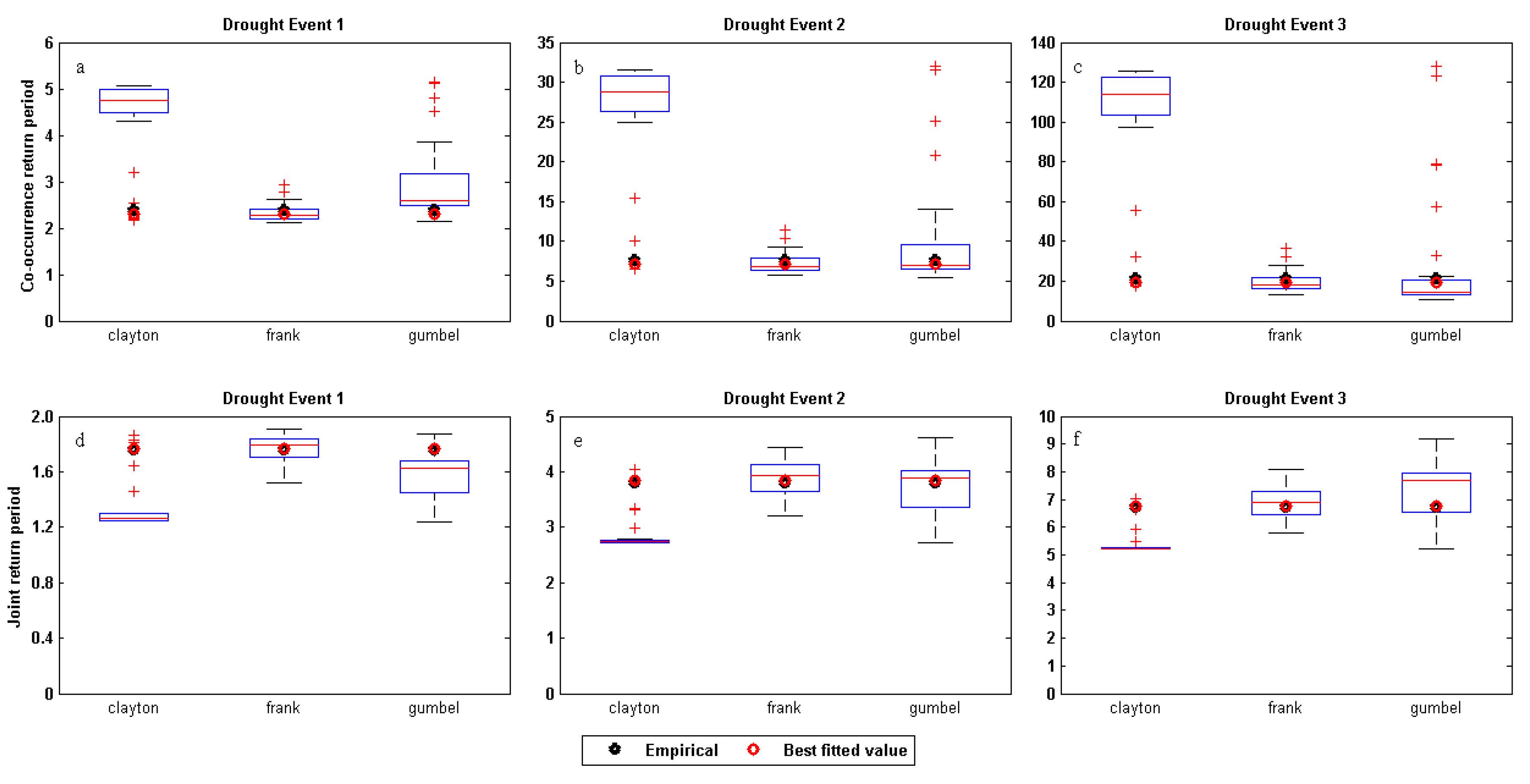
4.2. Effects of the Selection of Copula Functions to the Return Period

In order to analyze the difference between three copula functions, there are three drought samples (with a duration of 6.55 months and a severity of 1.04 mm (denoted by drought event 1), a duration of 9.27 months and a severity of 4.36 mm (denoted by drought event 2), and a duration of 10.90 months and a severity of 7.71 mm (denoted by drought event 3)) at Huaxian station. The co-occurrence return period and the joint return period based on 36 possible joint distributions of duration and severity, and with different Copula functions, are calculated for the three selected drought events at Huaxian station. Figure 9 are the boxplots and show their variability compared with the empirical values. For hydrological drought event 2, the co-occurrence return period ranges from 6.56 to 31.49 years for the Clayton copula, 5.71 to 11.41 years for the Frank copula, and 5.45 to 32.07 years for the Gumbel copula. There are large differences for the three copula functions. At Huaxian station, the best-fitted copula selected by marginal distributions GEV and GAM is the Frank copula, the co-occurrence return period of the best marginal distribution and best copula is 7.15 years, and the co-occurrence return period of the empirical value is 7.67 years. This indicates that the value of Frank, which is selected as the best copula function at Huaxian station, is nearest to the empirical values. In addition, the mean value of the Frank copula for 36 possible joint distributions are also near the empirical values. The same result is found in other two hydrological drought events, and the joint return period also shows the same situations.

4.3. Effects of Human Activities on Drought Frequency

The tendency of average annual runoff is decreasing at the three stations, especially, due to human activities, the observed runoff has significantly decreased in the period of 1991–2013 [7], which also shows that after 1991 human activities mainly resulted in the short-term drought fluctuation. In this study, because the main aim is to analyze the uncertainty of marginal distributions and copula functions on hydrological drought, we did not spilt the time series into two periods based on the turning point year. In addition, human activities affect the drought frequency in many ways. Irrigation area expansion means subtractions of water have greatly increased, which have resulted in the decrease of observed runoff [32]. The changing of land use has increased water demand, which has aggravated hydrological drought.

In addition, there are other uncertain factors, such as the selected threshold level of streamflow, climate change, and the length of time series. The threshold usually varies from $Q_{30}$ to $Q_5$ of streamflow, and drought events of higher severity are “nested” inside drought events of lower severity, such as a $Q_{10}$ threshold drought implying the occurrence of $Q_{20}$ and $Q_{30}$ threshold drought events. Under the changing climate, the precipitation series and runoff series are non-stationary; the surface runoff is not only sensitive to precipitation, but also sensitive to temperature [33]. The length of the times series determines the number of drought events. These uncertainty factors are not key points in this study, as we will discuss their effects on hydrological drought frequency in our next study.

5. Conclusions

This study investigated the regional drought frequency analysis in the Weihe River Basin considering the spatio-temporal structure of drought with copula functions. The primary conclusions are given as follows:

(1)

There are more drought events at Huaxian station (lower basin) than at Linjiacun station (upper basin), but there are longer drought durations and greater severity at Linjiacun station.

(2)

Based on the AD test, five models (EXP, GAM, LOGN, GEV, WBL) are acceptable for the fit of the drought duration and drought severity at LJC and XY stations. The GP model is not acceptable for the goodness-of-fit of drought duration and drought severity at three stations, the EXP model is rejected for the fit of drought severity at Huaxian station.

(3)

Based on ordinary least squares (OLS) and Akaike information criterion (AIC), the Frank copula is the best joint distribution function at Linjiacun and Huaxian stations, while the Clayton copula is the best-fitted model at Huaxian station.

(4)

The co-occurrence return period is greater than both the return periods defined by drought duration and drought severity separately, while the joint return period is shorter than both of the return periods. This shows that these two kinds of combination return periods can be regarded as two extreme conditions of the marginal distribution return period. It is possible to estimate the interval of the actual return period according to the co-occurrence return period and the joint return period.

(5)

The drought return period is sensitive to the selected marginal distribution and different copula functions. Therefore, it is important to select proper marginal distributions and copula functions, and the sensitivity and uncertainty of hydrological droughts should be paid more attention on the modeling and designing of drought models with consideration to the condition of water resources and the requirement of water management.

References

1. Tallaksen, L.M.; Van Lanen, H.A. Hydrological Drought: Processes and Estimation Methods for Streamflow and Groundwater; Developments in Water Science; Elsevier: Amsterdam, The Netherlands, 2004; Volume 48. [Google Scholar]
2. Tallaksen, L.M.; Hisdal, H.; Van Lanen, H.A. Space–time modelling of catchment scale drought characteristics. J. Hydrol. 2009, 375, 363–372. [Google Scholar] [CrossRef]
3. Van Loon, A.; Van Lanen, H. A process-based typology of hydrological drought. Hydrol. Earth Syst. Sci. 2012, 16, 1915. [Google Scholar] [CrossRef]
4. Nyabeze, W.R. Estimating and interpreting hydrological drought indices using a selected catchment in Zimbabwe. Phys. Chem. Earth A/B/C 2004, 29, 1173–1180. [Google Scholar] [CrossRef]
5. Byzedi, M.; Saghafian, B. Analysis of hydrological drought based on daily flow series. Proc. World Acad. Sci. Eng. Technol. 2010, 70, 249–252. [Google Scholar]
6. Jaranilla-Sanchez, P.A.; Wang, L.; Koike, T. Modeling the hydrologic responses of the pampanga river basin, philippines: A quantitative approach for identifying droughts. Water Resour. Res. 2011, 47, W03514. [Google Scholar] [CrossRef]
7. Ren, L.; Shen, H.; Yuan, F.; Zhao, C.; Yang, X. Hydrological drought characteristics in the Weihe catchment in a changing environment. Adv. Water Sci. 2016, 27, 492–500. [Google Scholar]
8. Yue, S. Applying bivariate normal distribution to flood frequency analysis. Water Int. 1999, 24, 248–254. [Google Scholar] [CrossRef]
9. Bacchi, B.; Becciu, G.; Kottegoda, N.T. Bivariate exponential model applied to intensities and durations of extreme rainfall. J. Hydrol. 1994, 155, 225–236. [Google Scholar] [CrossRef]
10. Yue, S.; Ouarda, T.; Bobee, B. A review of bivariate gamma distributions for hydrological application. J. Hydrol. 2001, 246, 1–18. [Google Scholar] [CrossRef]
11. Ganguli, P.; Reddy, M.J. Evaluation of trends and multivariate frequency analysis of droughts in three meteorological subdivisions of western India. Int. J. Climatol. 2014, 34, 911–928. [Google Scholar] [CrossRef]
12. Shiau, J. Fitting drought duration and severity with two-dimensional copulas. Water Resour. Manag. 2006, 20, 795–815. [Google Scholar] [CrossRef]
13. Sklar, M. Fonctions de Répartition à n Dimensions et Leurs Marges; Université Paris 8: Saint-Denis, France, 1959. [Google Scholar]
14. Hürlimann, W. Fitting bivariate cumulative returns with copulas. Comput. Stat. Data Anal. 2004, 45, 355–372. [Google Scholar] [CrossRef]
15. Michele, C.; Salvadori, G.; Vezzoli, R.; Pecora, S. Multivariate assessment of droughts: Frequency analysis and dynamic return period. Water Resour. Res. 2013, 49, 6985–6994. [Google Scholar] [CrossRef]
16. Khedun, C.P.; Mishra, A.K.; Singh, V.P.; Giardino, J.R. A copula-based precipitation forecasting model: Investigating the interdecadal modulation of ENSO’s impacts on monthly precipitation. Water Resour. Res. 2014, 50, 580–600. [Google Scholar] [CrossRef]
17. Nazemi, A.A.; Wheater, H.S. Assessing the vulnerability of water supply to changing streamflow conditions. Eos Trans. Am. Geophys. Union 2014, 95, 288. [Google Scholar] [CrossRef]
18. Tu, X.; Singh, V.P.; Chen, X.; Ma, M.; Zhang, Q.; Zhao, Y. Uncertainty and variability in bivariate modeling of hydrological droughts. Stoch. Environ. Res. Risk Assess. 2016, 30, 1317–1334. [Google Scholar] [CrossRef]
19. Genest, C.; Favre, A.-C. Everything you always wanted to know about copula modeling but were afraid to ask. J. Hydrol. Eng. 2007, 12, 347–368. [Google Scholar] [CrossRef]
20. Marsaglia, G.; Marsaglia, J. Evaluating the Anderson-Darling distribution. J. Stat. Softw. 2004, 9, 1–5. [Google Scholar] [CrossRef]
21. Wang, H.; Zhang, Z. Regulation on runoff and sediment discharge of main branches located in wei river valley and benefits of runoff and sediment decrease under control measures of soil and water conservation. Bull. Soil Water Conversat. 1995, 15, 55–59. [Google Scholar]
22. Song, J.; Xu, Z.; Liu, C.; Li, H. Ecological and environmental instream flow requirements for the Wei river—The largest tributary of the yellow river. Hydrol. Process. 2007, 21, 1066–1073. [Google Scholar] [CrossRef]
23. Yuan, F.; Ma, M.; Ren, L.; Shen, H.; Li, Y.; Jiang, S.; Yang, X.; Zhao, C.; Kong, H. Possible future climate change impacts on the hydrological drought events in the weihe river basin, China. Adv. Meteorol. 2016. [Google Scholar] [CrossRef]
24. Van Loon, A. On the Propagation of Drought: How Climate and Catchment Characteristics Influence Hydrological Drought Development and Recovery; Wageningen University: Wageningen, The Netherlands, 2013. [Google Scholar]
25. Fleig, A.K.; Tallaksen, L.M.; Hisdal, H.; Demuth, S. A global evaluation of streamflow drought characteristics. Hydrol. Earth Syst. Sci. 2006, 10, 535–552. [Google Scholar] [CrossRef]
26. Li, C.; Singh, V.P.; Mishra, A.K. A bivariate mixed distribution with a heavy-tailed component and its application to single-site daily rainfall simulation. Water Resour. Res. 2013, 49, 767–789. [Google Scholar] [CrossRef]
27. Genest, C.; Rémillard, B.; Beaudoin, D. Goodness-of-fit tests for copulas: A review and a power study. Insur. Math. Econ. 2009, 44, 199–213. [Google Scholar] [CrossRef]
28. Joe, H. Multivariate Models and Multivariate Dependence Concepts; CRC Press: Boca Raton, FL, USA, 1997. [Google Scholar]
29. Haan, C.T. Statistical Methods in Hydrology; The Iowa State University Press: Ames, IA, USA, 2002. [Google Scholar]
30. Bonaccorso, B.; Bordi, I.; Cancelliere, A.; Rossi, G.; Sutera, A. Spatial variability of drought: An analysis of the SPI in Sicily. Water Resour. Manag. 2003, 17, 273–296. [Google Scholar] [CrossRef]
31. Salvadori, G.; Durante, F.; De Michele, C. On the return period and design in a multivariate framework. Hydrol. Earth Syst. Sci. 2011, 15, 3293–3305. [Google Scholar] [CrossRef]
32. Fu, G.; Chen, S.; Liu, C.; Shepard, D. Hydro-climatic trends of the Yellow river basin for the last 50 years. Clim. Chang. 2004, 65, 149–178. [Google Scholar] [CrossRef]
33. Jin, H.; Liang, R.; Wang, Y.; Tumula, P. Flood-runoff in semi-arid and sub-humid regions, a case study: A simulation of jianghe watershed in northern China. Water 2015, 7, 5155–5172. [Google Scholar] [CrossRef]
Figure 1. The study basin map.
Water 09 00334 g001
Figure 2. Threshold level method with a variable threshold to define the drought duration and drought severity.
Water 09 00334 g002
Figure 3. Drought events in three stations during 1960–2012.
Water 09 00334 g003
Figure 4. The number events of different drought (a) durations and (b) severities at three stations.
Water 09 00334 g004
Figure 5. Marginal distribution modeling of drought duration and drought severity. (a): LJC drought duration; (b): XY drought duration; (c): HX drought duration; (d): LJC drought severity; (e): XY drought severity; (f): HX drought severity.
Water 09 00334 g005
Figure 6. Probability-probability (PP) plot of the joint distributions of duration-severity at three stations. (a): LJC; (b): XY; (c): HX.
Water 09 00334 g006
Figure 7. Co-occurrence return period and joint return period of the best-selected copula. (a): LJC drought duration; (b): XY drought duration; (c): HX drought duration; (d): LJC drought severity; (e): XY drought severity; (f): HX drought severity.
Water 09 00334 g007
Figure 8. The return period of drought duration and severity based on different marginal distributions at three stations. (a): LJC drought duration; (b): XY drought duration; (c): HX drought duration; (d): LJC drought severity; (e): XY drought severity; (f): HX drought severity.
Water 09 00334 g008
Figure 9. Sensitivity of the co-occurrence return period and joint return period of three drought events at Huaxian station and the selection of the univariate distribution and the copulas. (a): co-occurrence return period of drought event 1; (b): co-occurrence return period of drought event 2; (c): co-occurrence return period of drought event 3; (d): joint return period of drought event 1; (e): joint return period of drought event 2; (f): joint return period of drought event 3.
Water 09 00334 g009