Comparison of Spatial Interpolation Schemes for Rainfall Data and Application in Hydrological Modeling

Abstract

The spatial distribution of precipitation is an important aspect of water-related research. The use of different interpolation schemes in the same catchment may cause large differences and deviations from the actual spatial distribution of rainfall. Our study analyzes different methods of spatial rainfall interpolation at annual, daily, and hourly time scales to provide a comprehensive evaluation. An improved regression-based scheme is proposed using principal component regression with residual correction (PCRR) and is compared with inverse distance weighting (IDW) and multiple linear regression (MLR) interpolation methods. In this study, the meso-scale catchment of the Fuhe River in southeastern China was selected as a typical region. Furthermore, a hydrological model HEC-HMS was used to calculate streamflow and to evaluate the impact of rainfall interpolation methods on the results of the hydrological model. Results show that the PCRR method performed better than the other methods tested in the study and can effectively eliminate the interpolation anomalies caused by terrain differences between observation points and surrounding areas. Simulated streamflow showed different characteristics based on the mean, maximum, minimum, and peak flows. The results simulated by PCRR exhibited the lowest streamflow error and highest correlation with measured values at the daily time scale. The application of the PCRR method is found to be promising because it considers multicollinearity among variables.

1. Introduction

The spatial distribution of precipitation plays an important role in hydrological modeling, disaster prediction, and watershed management. Many uncertain factors, including topographic factors such as latitude, longitude, altitude, slope, aspect, and large-scale circulation, have variable effects on the spatial distribution of precipitation. Therefore, it is necessary to conduct a detailed study to improve the accuracy of such analyses. Spatial interpolation schemes are required to provide accurate spatial distributions of rainfall. Various interpolation methods have been developed for this purpose, ranging from simple techniques such as Thiessen polygons [1] and inverse distance weighting schemes [2] to complex statistical methods such as multiple linear regression [3] and geostatistical kriging [4,5]. The more complex approaches use additional information such as elevation, slope, or radar-estimated rainfall as covariates [6]. Recently, soft computing schemes have been used to perform spatial interpolation for environmental variables. The methods such as support vector machine [7] and artificial neural network (ANN) [8] were used, and the methods need no prior knowledge and assumptions. A Fuzzy system was introduced to consider the interpretability of the spatial interpolation models [9]. The interpolation method is more diverse and can be selected according to different watershed conditions. For the application of spatial interpolation, most studies have used only monthly or annual time steps for precipitation interpolation and mapping [10]. A part of the research has focused on the use of geostatistical and non-geostatistical approaches for the interpolation of daily rainfall in different sizes of area (Kyriakidis et al. [11], Buytaert et al. [4]). Only a small number of studies have considered using hourly time steps for large-scale extreme rainfall events, e.g., Schiemann et al. [6] used a geostatistical radar-rain gauge combination correlograms and semi-variogram models for the construction of hourly precipitation grids for Switzerland. A few studies have comprehensively compared the spatial interpolation methods from the annual, daily, and hourly scales.

Spatial interpolation schemes, based on multiple regression with residual correction are useful because they utilize geographic information to interpolate the precipitation data from rain gauge stations. Thus, multiple regression residuals are spatially interpolated. Several studies have used such methods for interpolating spatial precipitation. Ninyerola [12] applied spatial interpolation tools to map monthly precipitation on the Iberian Peninsula, and the most accurate results were obtained using a global model with multiple regression mixed with spline interpolation of the residuals. Agnew and Palutikof [13] used multiple regression models that were refined by kriging of the residuals to develop seasonal maps of temperature and precipitation in the Mediterranean basin. Latitude, elevation, and distance from the sea were found to be the most effective predictors of local seasonal climate, while the overall estimation efficiency of the models was high. Haralambos [14] applied a backward stepwise multiple regression with topographical and geographical parameters, including the normalized difference vegetation index (NDVI), as independent variables in a regression equation to model temperature and precipitation data in Greece. Luo et al. [15] used four spatial interpolation methods for monthly precipitation interpolation. The result showed that Ordinary Co-Kriging (OCK) and Ordinary Kriging (OK) performed better than other two methods, and finally the author integrated OK and OCK based on their respective superiority and obtained the results with less error than those of OK and OCK. However, most studies that have used multiple regression with residuals have focused on mapping annual or seasonal precipitation distributions and have only applied interpolation schemes at annual or monthly scales. These limitations represent a lack of a systematic and comprehensive evaluation of the performance of such methods. In addition, when several variables are used to construct multivariate linear regression models of precipitation, multicollinearity may exist between variables. Some studies have used stepwise regression models, which can select important variables related to precipitation and exclude the less important variables; however, some geographic information will be lost.

Cross-validation is a common technique used to evaluate interpolation results [16,17]. Unfortunately, the accuracy of this validation method depends on the number and the locations of gauges within the study area, which should be representative of the spatial distribution of rainfall [18]. Haberlandt et al. [19] proposed a method for comparing spatial interpolation methods using not only internal precipitation validation but also objective verification based on streamflow simulations to produce and compare various time series of daily precipitation distributions. The approach of using a hydrological model to validate the performances of different interpolation schemes has been used in several studies. Ruelland et al. [20] analyzed the sensitivity of a lumped and semi-distributed hydrological model for several spatial interpolations of rainfall data. Wagner [10] used regression-based interpolation approaches with the two most suitable covariates in a meso-scale catchment of India based on a Soil and Water Assessment Tool (SWAT) model for simulating catchment runoff. The author concluded that choosing a suitable interpolation scheme should not only be based on the comparison of measured values at points but should also consider the given measurement network and the interpolated spatial rainfall distribution.

The main objective of this paper is to propose a principal component regression (PCR) with a residual correction spatial interpolation scheme and compare it with several traditional methods on annual, daily, and hourly scales. Cross-validation is applied for all three time scales, and the Hydrologic Modeling System (HEC-HMS) hydrological model is used to evaluate runoff and describe the temporal and spatial distributions of rainfall at daily and hourly time steps.

2. Materials and Methods

2.1. Study Area

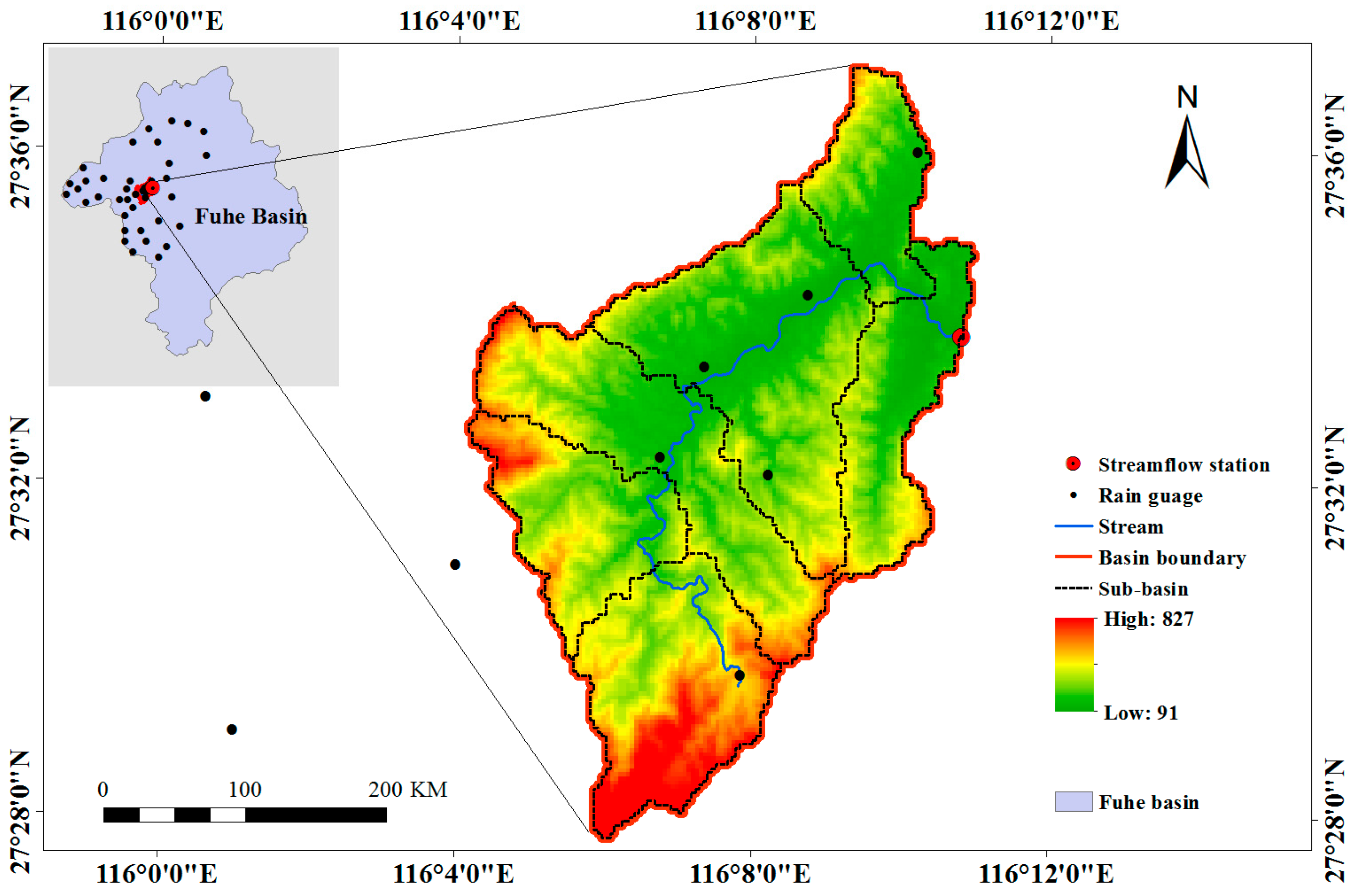
The Xinxie catchment (27.54° N~27.57° N, 116.10° E~116.15° E; Figure 1) is located in southeastern China and is a tributary of the Fuhe River. The drainage area of the Xinxie catchment is 96.4 km². The elevation ranges between 92 m and 827 m and increases gradually from north to south. The catchment is dominated by a tropical monsoon climate, and mean annual temperature, precipitation, and runoff are 17.5 °C, 1866.5 mm, and 1017.3 mm, respectively. Precipitation is mainly concentrated from May through September (69.8% of annual precipitation and 66.6% of annual runoff). The soil texture in the watershed is mainly sandy clay and clay loam.

2.2. Data

The data used in this study include information used for spatial interpolation and input forcing in hydrological modeling. Daily and hourly measurements of precipitation at 41 gauges within (seven gauges) or close to the catchment (34 gauges) and streamflow records from the Xinxie hydrological station situated at the outlet of the Xinxie basin (Figure 1) were provided by the Hydrology Bureau of Jiangxi Province from 2007 to 2013. Geographic information was obtained as follows. A 90 m digital elevation model (DEM) was obtained from the Shuttle Radar Topography Mission (SRTM), soil types were obtained from the 5-min Food Agriculture Organization (FAO) dataset [21], and land cover data were provided by the Chinese Academy of Science.

Table 1. Data for interpolation and model application.

Spatial Interpolation	Methods	Precipitation at 41 Gauges	Lat & Lon	Elevation	Slope	Aspect
	IDW	√	√
	MLR	√	√	√
	PCRR	√	√	√	√	√
Model Application	All three methods	streamflow records at Xinxiel station	soil types	land cover data

shows the data for interpolation and model application.

Data Preprocessing

Hydrometeorological data sets often include measurement and recording errors, which affect the interpolation results. In this study, daily precipitation data at 41 rainfall stations were tested using double mass curves [22], and the data from the Xinxie station were selected as the reference because daily precipitation data were continuous from 2007 to 2013. The cumulative sum of precipitation at each other station was compared with that at the reference station daily, and if the double cumulative curve exhibited an inconsistency, the data were checked and suspect data were flagged as missing. Then, the missing values were filled using a regression-based interval filling method [23]. The corresponding annual precipitation sums were calculated for every gauge using the same dates; thus, relationships were established between the incomplete data and data at other stations based on linear regression.

2.3. Interpolation Schemes

In this study, the principal component regression with the residual correction (PCRR) method, the inverse distance square (IDW) method, and the multiple linear regression (MLR) method were used to compare interpolated annual, daily, and hourly precipitation and the spatial distribution of precipitation in the Xinxie catchment. In addition, the interpolation results were used as input data in a hydrological model at daily and hourly time scales. These interpolation schemes were performed using a 500 m × 500 m grid, and inputs for the HEC-HMS hydrological model were based on this grid by averaging the values in each sub-basin. The specific interpolation schemes are as follows.

2.3.1. Principal Component Regression with Residual Correction

MLR is one of the common methods of spatial precipitation interpolation. Hay et al. [24] used MLR to spatially interpolate precipitation for simulating runoff in the Animas River basin of southwestern Colorado; the gridded values of precipitation provide a physically based estimate of the spatial distribution of precipitation and result in reliable simulations of daily runoff in the Animas River basin. The traditional MLR method assumes that a linear relationship exists between the predictor variables and a known response variable. The latitude, longitude, and elevation data from meteorological stations can be used to establish a regression model [25]. However, MLR estimation is unsatisfactory under some conditions. For example, the column vectors of matrix X may be near-linearly correlated. The approximate linear relationship between the independent variables is called multicollinearity, and the existence of multicollinearity is the main reason for inconsistencies between the sign and the value of the calculated regression coefficient and the actual sign and value. Principal component regression (PCR) was proposed by Massy [26] in 1965 based on principal component analysis (PCA). By linear transformation, the original indicators are combined into a few independent indicators that fully reflect the associated information. This approach avoids collinearity between variables and preserves important information. Therefore, the response variables (dependent variables) can be regressed based on these principal components, and then the estimation equation of the original regression model can be obtained according to the relationship between the principal components and explanatory variables (independent variables). The specific steps of PCR are not repeated here; see Massy [26] and Rocha [27].

The main component of this method is adding macroscopic and microscopic topographic factors as covariates to construct the PCR model of rainfall station precipitation based on station latitude and longitude, elevation, slope, and slope aspect. Then, we calculate the regression coefficient and simulate the regression grid surface. The residual value is obtained by subtracting the interpolated value from the measured value, and the residual is interpolated using the IDW method. Finally, the meteorological data grid surface is formed by summation with the regression grid surface. We call this the principal component regression with residual (PCRR) analysis method. The PCRR method considers the influence of terrain on meteorological data and the multicollinearity between variables, which is a new improvement to traditional methods of meteorological data interpolation. The PCRR method uses slightly different data processing methods at three time scales. The specific operations are as follows.

Annual Precipitation Interpolation

(1) The precipitation data from the meteorological stations used in the regression calculations are taken as dependent variables, and the longitude, latitude, altitude, slope, and slope aspect of the meteorological stations are used as input variables to perform PCR. To make the regression model more accurate and more comprehensive for simulating the spatial variations in precipitation in the new oblique basin, a regression analysis was conducted by adding 35 rainfall stations around the basin. The regression coefficients ${\widehat{b}}_0$, ${\widehat{b}}_1$, ${\widehat{b}}_2$, ${\widehat{b}}_3$, ${\widehat{b}}_4$, and ${\widehat{b}}_5$ were calculated using the formula below:

$$\widehat{Y}={\widehat{b}}_0+{\widehat{b}}_1{X}_1+{\widehat{b}}_2{X}_2+{\widehat{b}}_3{X}_3+{\widehat{b}}_4{X}_4+{\widehat{b}}_5{X}_5$$

(1)

where $\widehat{Y}$ is the value of precipitation and $X_1$, $X_2,X_{3,}{X}_4$, and $X_5$ represent the longitude, latitude, altitude, slope, and aspect of the meteorological station, respectively.

(2) The latitude, longitude, slope, aspect, and DEM grid surfaces are substituted into the regression equation to obtain the regression grid surface of the meteorological data:

$${\widehat{Y}}_S={\displaystyle \sum }_{i=1}^n({\widehat{b}}_0+{\widehat{b}}_1{X}_{1i}+{\widehat{b}}_2{\mathrm{X}}_{2i}+{\widehat{b}}_3{X}_{3i}+{\widehat{b}}_4{X}_{4i}+{\widehat{b}}_5{X}_{5i})$$

(2)

where ${\widehat{Y}}_S$ is the regression grid surface of meteorological data and X_1i, X_2i, X_3i, $X_{4i},\mathrm{and}{X}_{5i}$ are the ith (i = 1, 2,..., n) grid cell values of the longitude, latitude, altitude, slope, and aspect grid surfaces.

(3) The interpolated values at stations and observed values used to train sample points differ. Thus, a residual exists:

$$p_{ri}=p_{oi}-p_{si}$$

(3)

where $p_{ri}$ is the residual value of the precipitation data at the ith meteorological station, $p_{oi}$ is the value of annual mean precipitation at the ith meteorological station, and $p_{si}$ is the regression value of the ith meteorological station extracted from the grid surface of the meteorological data regression.

(4) The residual value of precipitation data is interpolated into a grid surface based on IDW:

$${\widehat{Y}}_R=\frac{{\sum }_{i=1}^n\frac{1}{{\left(d_i\right)}^p}{P}_{ri}}{{\sum }_{i=1}^n\frac{1}{{\left(d_i\right)}^p}}$$

(4)

where ${\widehat{Y}}_R$ is the residual grid surface of meteorological data, P_ri is the residual value of ith meteorological station, n is the number of stations used for the interpolation of residual values, $d_i$ is the distance from the interpolated point to the ith meteorological station, and P is the power of the distance.

(5) The final grid surface of the precipitation data is calculated as follows:

$$Y_F={\displaystyle \sum }_{i=1}^n({\widehat{Y}}_{Si}+{\widehat{Y}}_{Ri})$$

(5)

where $Y_F$ is the final grid surface of the precipitation data, ${\widehat{Y}}_{Si}$ is the ith grid cell value of the regression grid surface of the precipitation data, and ${\widehat{Y}}_{Ri}$ is the ith grid cell value of the residual grid surface of the precipitation data.

Daily Precipitation Interpolation

(1) When using the PCRR method for daily precipitation interpolation, due to the selection of 35 rainfall stations outside the catchment as auxiliary regression sites, the first step is to determine the number of rainy days. If the precipitation in the Xinxie catchment is 0, the day is considered a non-precipitation day and the regression analysis is not performed; otherwise, we proceed to the second step.

Steps (2) to (6) are the same as Steps (1) to (5) in the ‘Annual Precipitation Interpolation’ section and will not be repeated here.

Hourly Precipitation Interpolation

The hourly precipitation interpolation in this study focuses on a flood event. Such an event reflects the hydrological process from the beginning of rainfall to the flood recession at the outlet of the catchment, the Xinxie hydrological station. Therefore, to avoid the effect of spatial precipitation variability associated with a flood event, only the rainfall gauges located inside the Xinxie catchment are selected for regression analysis. The remaining steps are the same as those in ‘Annual Precipitation Interpolation’ and will not be repeated here.

2.3.2. Multiple Linear Regression

The MLR method was described in the PCRR Section above and will not be repeated here. Data processing using the MLR method is the same as that in the PCRR method on all three time scales.

2.3.3. Inverse Distance Weighting

IDW is a widely used method for the estimation of missing data in hydrology and geographical sciences. Robinson and Metternich [28], in their study testing the performance of spatial interpolation techniques for mapping soil properties, have used the IDW method and concluded that IDW is able to interpolate subsoil pH with a sensible accuracy. The influence of a measured point is weighted according to the distance from the sampled point to the estimated point. The formula for the IDW method is as follows:

$$Z\left(S_0\right)={\displaystyle \sum }_{i=1}^N{\lambda }_{i}Z\left(S_i\right)$$

(6)

where $Z\left(S_0\right)$ represents the interpolated value at point $S_0$, $Z\left(S_i\right)$ represents the observed value at point $S_i$, n is the number of observations, and ${\lambda }_i$ is the weight. The weights ${\lambda }_i$ can be calculated as follows:

$${\lambda }_i=\frac{{d_{i0}}^{-p}}{{\sum }_{i=1}^N{d_{i0}}^{-p}},{\displaystyle \sum }_{i=1}^N{\lambda }_i=1$$

(7)

where $p$ is a power and $d_{i0}$ is the distance between a target and observations. The IDW method uses the same data processing procedure on all three time scales.

2.4. Hydrological Model

In this study, the Hydrologic Engineering Center Hydrologic Modeling System (HEC-HMS) model is used to evaluate the effects of different precipitation interpolation methods on runoff. The HEC-HMS model has been developed by the US Army Corps of Engineers [29] and can be used for many hydrological simulations such as simulations of natural rainfall-runoff processes or rainfall-runoff processes constrained by artificial controls. The HEC-HMS model is a semi-distributed model, which takes into account the spatial changes of the climate-environment and the underlying surface in the catchment. The catchment is divided into several sub-catchments using the natural divide line formed by the terrain, and various runoff calculation methods, basic flow calculation methods, and river channel confluence calculation methods can be adopted for each sub-basin and river channel respectively. The different parameters of each sub-catchment are set up, the runoff process and the slope convergence process of each sub-catchment are calculated, these are calculated along the river channel of confluence to the downstream control section outlets, and the hydrological elements such as the peak runoff, runoff, and peak time are calculated at the outlet of the catchment. The HEC-HMS model consists of four modules; namely, Basin Model, Meteorological Model, Control Specification, and Time-series Data. For a specific introduction of the HEC-HMS model see Feldman [29].

The HEC-HMS model has been validated in previous studies and has shown good applicability in catchments in Jiangxi Province [30,31]. Based on 90-m SRTM DEM data, HEC-GeoHMS, the preprocessing software of HEC-HMS, was used in this study to generate the basin boundary and river network of the Xinxie catchment, and the important terrain information in the typical small catchment was extracted (such as river length, riverbed gradient, maximum flow path length, etc.). The sub-catchment area was divided by the geographical location of the rainfall station in the study area. Based on the land use and soil texture data provided by the Jiangxi Freshet Torrent Project Management Office, the land use and soil texture characteristics of each small catchment were determined to provide basic underlying surface data for the determination of important physical parameters in HEC-HMS. Several parameterization schemes for the Xinxie catchment were selected in the catchment module of HEC-HMS (

Table 2. Hydrologic Engineering Center Hydrologic Modeling System (HEC-HMS) simulation scheme of Xinxie catchment.

Runoff-Volume Model	Direct-Runoff Model	Baseflow Model	Routing Model
Soil moisture accounting	Clark’s unit hydrograph	Linear reservoir	Lag

), and corresponding numerical simulation schemes were developed. The details of each step will not be repeated here.

In this paper, the Xinxie catchment was divided into six sub-basins (Figure 1), and the hydrological model was constructed according to the simulation parameterization scheme discussed above. Then, daily precipitation data from 2007 to 2013 and flood event data from each sub-basin were interpolated using the PCRR method, MLR method, and IDW method as input data used to drive the model (The flood event data refers to the flow record data and precipitation data recorded during a flood event from the rising time to the recession time. Usually as a result of storage effect of basin, the precipitation has occurred before the flood rises so the rising time often starts from the moment of precipitation). Some of the parameters of the HEC-HMS model need to be calibrated according to the historical rainfall runoff data; the criterion for parameter calibration is to find the optimal fit for the flow calculated by the parameter values and the measured flow at the outlet of the watershed. In this study, the genetic algorithm was used to automatically calibrate the model parameters to determine the maximum certainty coefficient as the objective function. This parameterization process has been successfully applied in the ‘Flash Flood Forecasting and Disaster Management of Jiangxi Province’ (grant No. 0628-156104104417) project.

2.5. Validation

(i) Cross-validation [32] was done to verify the effect of interpolation from 2007 to 2013 by eliminating the observation site data systematically. Other site data were used to generate the predicted values of the site, and the predicted values were compared with measured values to analyze the error associated with the interpolation. Mean absolute error (MAE), mean relative error (MRE), and root mean square error (RMSE) were used as the criteria to evaluate different interpolation methods. Their expression of the criteria are as follows:

$$\mathrm{RMSE}=\sqrt{\frac{{\sum }_{i=1}^N{(M_i-O_i)}^2}{N}}\mathrm{MAE}=\frac{{\sum }_{i=1}^N\mathrm{ABS}(M_i-O_i)}{N}\mathrm{MRE}=\frac{1}{N}{\displaystyle {{\displaystyle \sum }}_1^N}\left|\frac{\mathrm{ABS}\left(M_i-O_i\right)}{O_i}\right|$$

(8)

where $O_{\mathrm{i}}$ is the ith observation value, $M_i$ is the ith predicted value, and N is the total number of observations.

Errors can reflect the merits of calculation results from different perspectives. Among them, the MAE reflects the error range of the calculated values, and the error is given quantitatively. MRE gives the error range of the calculated values by reflecting the relative errors of different data sets, and the effect is intuitive. Moreover, RMSE can reflect the interpolative sensitivity and extreme effects associated with sample data.

(ii) Another method of comparing different spatial interpolation methods is to compare various time series of daily areal precipitation distributions using not only internal validation but also objective verification based on streamflow simulations [33]. Therefore, HEC-HMS was used to evaluate the effect of the different interpolation inputs on the water balance and runoff dynamics. The evaluation criteria include the percentage bias (PBIAS) and the Nash–Sutcliffe efficiency (NSE) [34]

$$\mathrm{NSE}=1-\frac{{\sum }_{i=1}^N{\left(O_i-M_i\right)}^2}{{\sum }_{i=1}^N{\left(O_i-\overline{O}\right)}^2}\mathrm{PBIAS}=100\cdot \frac{{\sum }_{i=1}^N{\left(O_i-M_i\right)}^2}{{\sum }_1^N{O}_i}$$

(9)

where $\overline{O}$ is the mean of the observed value and other notations are as defined above.

3. Results

Before analyzing the interpolation results of different schemes at different scales, a collinearity analysis was performed based on the MLR method. The matrix ${\mathit{X}}^{\mathit{T}}\mathit{X}$ of the observed data of the independent variables was analyzed, and various indexes were used to reflect the co-linearity between independent variables. Commonly used collinear diagnostic statistics include eigenvalues and condition indexes, etc. [35]. If the eigenvalues of matrix ${\mathit{X}}^{\mathit{T}}\mathit{X}$ displays the following relationship ${\mathit{d}}_{\mathbf{1}}\ge {\mathit{d}}_{\mathbf{2}}\ge \cdots \ge {\mathit{d}}_{\mathit{k}}$, then the conditional index $\frac{{\mathit{d}}_{\mathbf{1}}}{{\mathit{d}}_{\mathit{k}}}$ of X is used to characterize its singularity. Thus, $\frac{{\mathit{d}}_{\mathbf{1}}}{{\mathit{d}}_{\mathit{k}}}\left(\mathit{j}=\mathbf{1},\mathbf{2},\cdots ,\mathit{k}\right)$ is also called a conditional index. It is generally believed that if the conditional index is between 10 and 30, a weak correlation exists between the independent variables. Additionally, a value between 30 and 100 represents a moderate correlation, and a value greater than 100 denotes a strong correlation. The larger the condition index is, the closer the eigenvalue is to zero and the stronger the collinear relationship. The results of the collinearity analysis show that the eigenvalues are close to zero and the condition indexes are large in two dimensions, which suggests that multicollinearity exists between the independent variables when the MLR method is applied (

Table 3. Collinearity Diagnosis of the Multiple Linear Regression (MLR) method.

Dimension	Eigenvalue	Condition Index	Variance Proportions
			(Constant)	Longitude	Latitude	Elevation	Slope	Aspect
1	4.984468	1	0.00	0.00	0.00	0.01	0.01	0.01
2	0.662792	2.742335847	0.00	0.00	0.00	0.07	0.22	0.02
3	0.185079	5.189568491	0.00	0.00	0.00	0.07	0.08	0.82
4	0.167639	5.452825175	0.00	0.00	0.00	0.55	0.68	0.09
5	2.03 × 10−5	495.2502822	0.03	0.02	0.99	0.30	0.01	0.01
6	1.57 × 10−6	1781.863642	0.97	0.98	0.01	0.00	0.01	0.05

). However, this phenomenon can be avoided by using the PCRR method.

3.1. Annual Analysis

The results of data cross-validation for different interpolation schemes are shown in

Table 4. Cross-validation performance and ranking of different interpolation schemes for simulating annual precipitation.

Interpolation Scheme	Mean RMSE	Rank of Mean RMSE	Mean MAE	Rank of Mean MAE	Mean MRE (%)	Rank of Mean MRE
PCRR	40.1	1	31.2	1	1.51	1
IDW	53.1	2	39.4	2	1.98	2
MLR	54.0	3	41.2	3	2.19	3

. In general, the PCRR interpolation scheme was superior to other methods.

For annual precipitation, the MAE, MRE, and RMSE values of the eight interpolation methods exhibited similar trends.

On the whole, the PCRR scheme was used to calculate the relationship between precipitation and geographical factors such as latitude, longitude, elevation, and others via principal component regression. The interpolation effect of PCRR was superior to those of the other two methods for all indicators. The performance of the MLR method was slightly worse than that of the IDW method. Among all three schemes, RMSE ranged from 40.1 mm to 54 mm with relatively large variations. Additionally, MAE ranged from 31.2 mm to 41.2 mm, and MRE ranged from 1.51% to 2.19% with moderate variations.

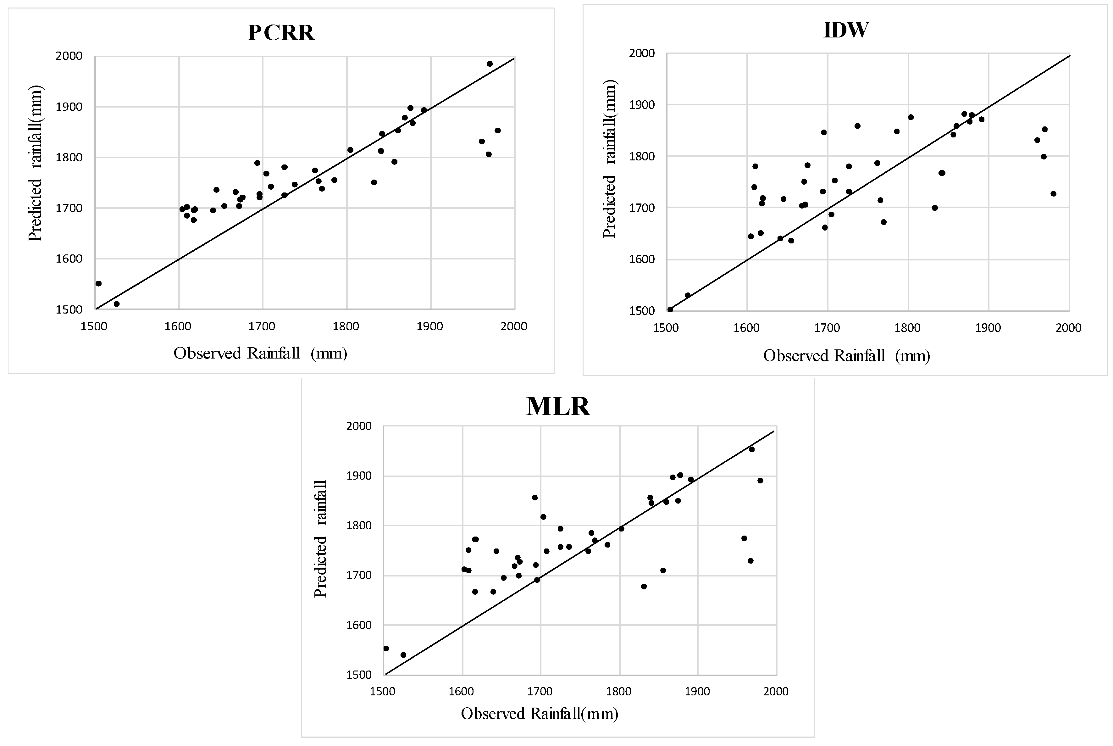
When evaluating the plots of observed versus predicted mean annual rainfall for each gauge from 2007 to 2013 (Figure 2), certain trends can be identified. Figure 2 shows that the PCRR method exhibits a good correlation between predicted precipitation and measured precipitation, and the points are located close to the 45-degree line; however, the correlation between the IDW method and the MLR method is low. The PCRR scheme displayed good performance due to the addition of a variety of terrain elements and the consideration of multicollinearity between the independent variables. In addition, the residuals were further processed in the PCRR method. As shown in Figure 2, further analysis of three schemes suggests that the annual mean precipitation ranged from 1500 to 2000 mm, and the predicted values were slightly larger than the measured values when the annual precipitation was less than 1800 mm, i.e., an overestimation trend was present. Additionally, the predicted values were less than the measured values when the annual precipitation was more than 1800 mm, which reflects an underestimation trend.

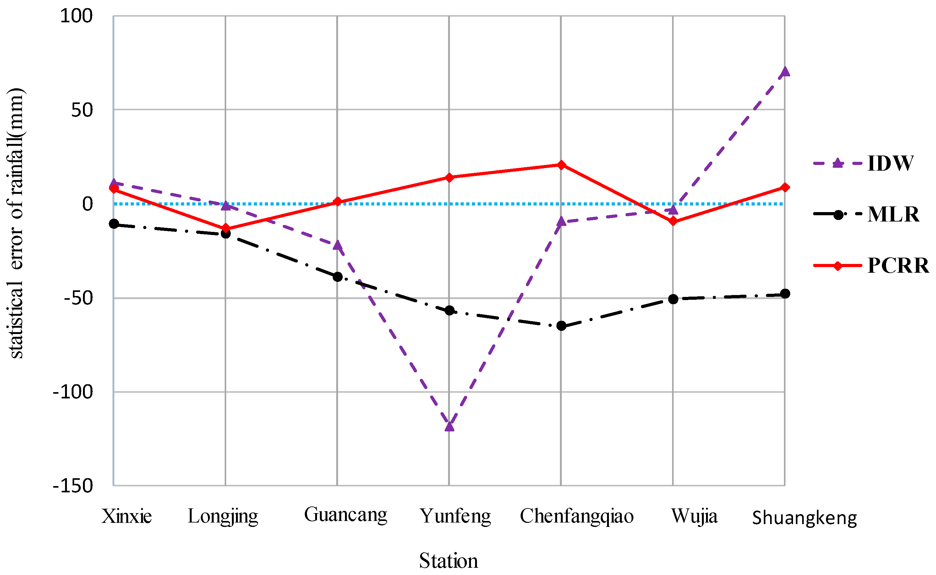
According to the above results, the statistical error (SE) of each station (Figure 3) reflects regional interpolation trends. The $\pm$SE range of the PCRR method at all stations was 20.5 mm, and five of the seven stations had SE values greater than 0 mm. Notably, the SE values of the IDW method displayed a significant negative trend at Yunfeng station, which is the southernmost station in the catchment. The average annual precipitation at Yunfeng station was 1970.5 mm, which exceeds 1800 mm; thus, this trend is consistent with previous conclusions that the predicted values are underestimated. The MLR method yielded negative SE values at all stations, which is opposite to the results of the PCRR method. This phenomenon is because the annual precipitation at all stations in the Xinxie catchment was more than 1800 mm, while only seven out of the 34 sites outside the basin had an annual precipitation greater than 1800 mm. Thus, the regression model using precipitation as the objective function is not ideal for extreme values. Since the PCRR residuals were further interpolated, the degree of negative correlation is the smallest among the three methods, thus the addition of a residual can effectively avoid the systematic deviations in predictions.

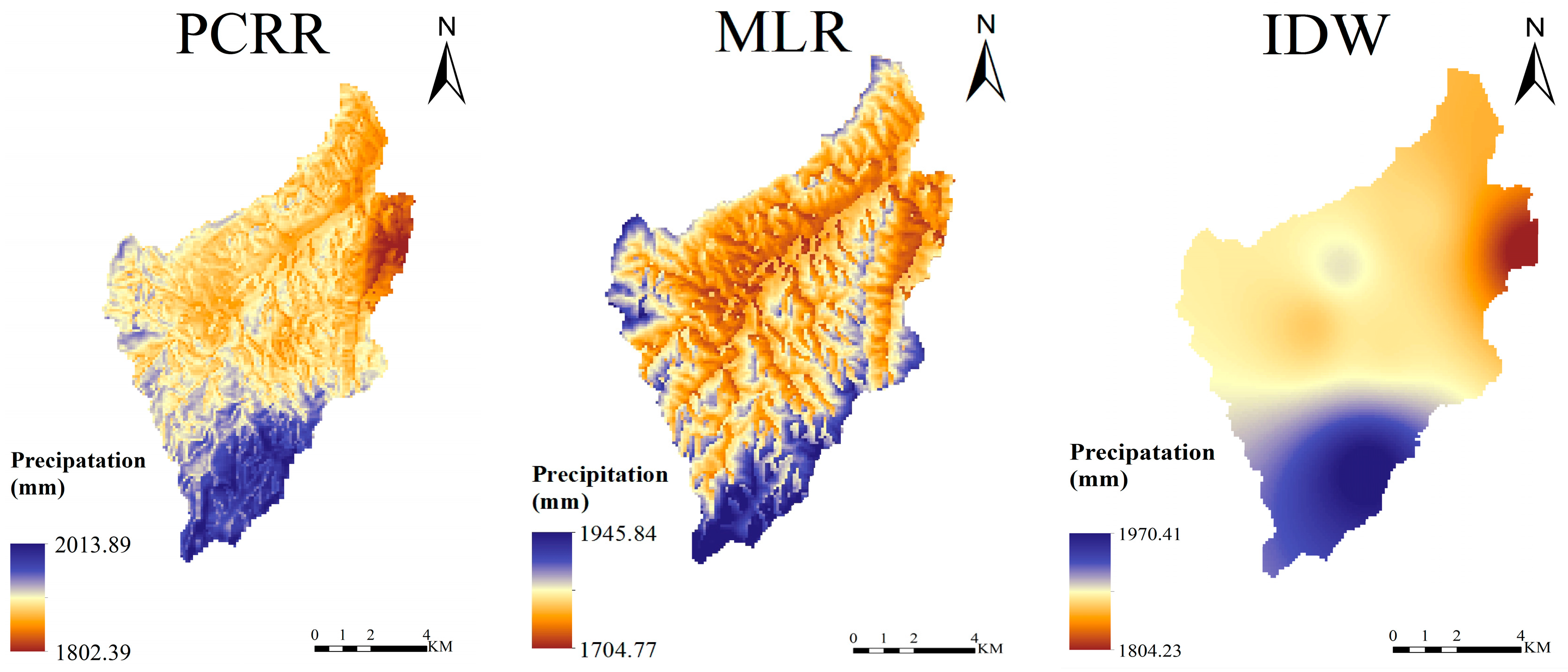
Spatial maps generated from each interpolation method (Figure 4) were used to visualize some of the spatial patterns of annual rainfall in the Xinxie basin from 2007 to 2013. The spatial distribution of precipitation and the elevation of the catchment increased from north to south. These results suggest that the precipitation is affected by topography. As shown in the simulation results of the three interpolation methods, the IDW method produced obvious circles around the interpolation points. Additionally, the PCRR and MLR schemes accounted for more micro-scale changes in rainfall, while the IDW interpolation method displayed a clear dividing line. Overall, the simulation results of the PCRR scheme were satisfactory. Because of its high simulation accuracy, the zonal distribution of precipitation in space was clearly reflected in the map and was consistent with the actual distribution.

3.2. Daily Analysis

Daily precipitation from 2007 to 2013 was interpolated using the PCRR, IDW, and MLR schemes. The results of cross-validation show that the PCRR scheme performed better than the other two schemes, and the differences between the indicators of different methods on the daily scale were more obvious than those on the annual scale (

Table 5. Cross validation performance and ranking of different interpolation schemes for simulating daily precipitation.

Interpolation Scheme	Mean RMSE	Rank of Mean RMSE	Mean MAE	Rank of Mean MAE	Mean MRE	Rank of Mean MRE
PCRR	3.92	1	3.06	1	0.49	1
IDW	8.38	2	6.63	2	1.17	2
MLR	12.39	3	10.55	3	1.81	3

), which suggests that the spatial variability of daily precipitation was larger than that of annual precipitation.

Another way to compare the spatial interpolation methods is to produce and compare various time series of daily areal precipitation distributions using not only internal precipitation validation but also objective verification based on streamflow simulations [36].

Table 6. Model performance using differently interpolated rainfall inputs.

Interpolation Scheme	Annual Precipitation (mm)		Measured (mm)	Simulated (mm)	Absolute Error (mm)	Relative Error (%)	NSE
	Simulated	Measured
PCRR	1875.5	1919.0	979.6	975.1	−4.5	−0.46	0.806
IDW	1872.9		979.6	930.2	−49.4	−5.04	0.803
MLR	1740.0		979.6	880.1	−99.5	−10.15	0.707

shows the HEC-HMS daily runoff performance using different interpolated rainfall inputs in the Xinxie catchment from 2007 to 2013. The results showed that the PCRR model yielded the minimum relative error in average annual runoff depth (0.97%). Additionally, the NSE coefficient obtained using the IDW method was slightly lower than that of the PCRR method (0.803), and the relative error associated with the average annual runoff depth was 5.34%. Due to the underestimation of precipitation by the MLR method, the average annual relative error and the NSE coefficient were unsatisfactory.

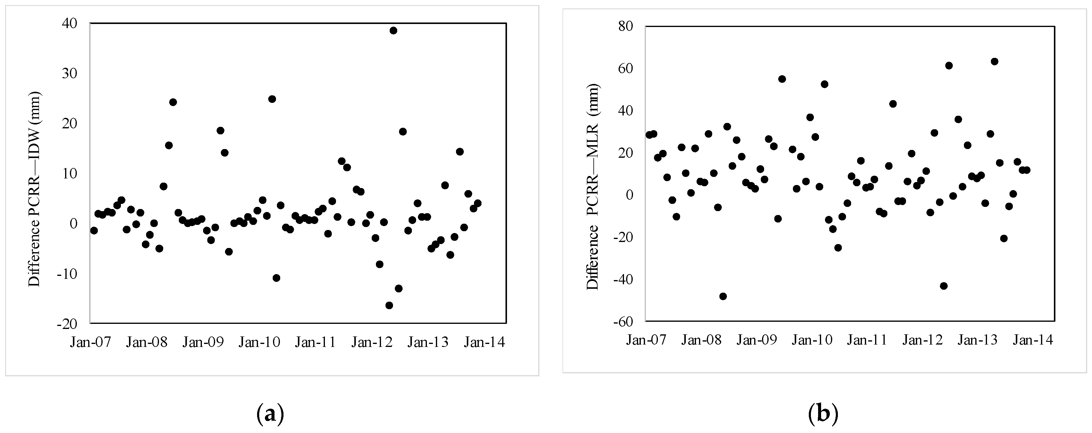
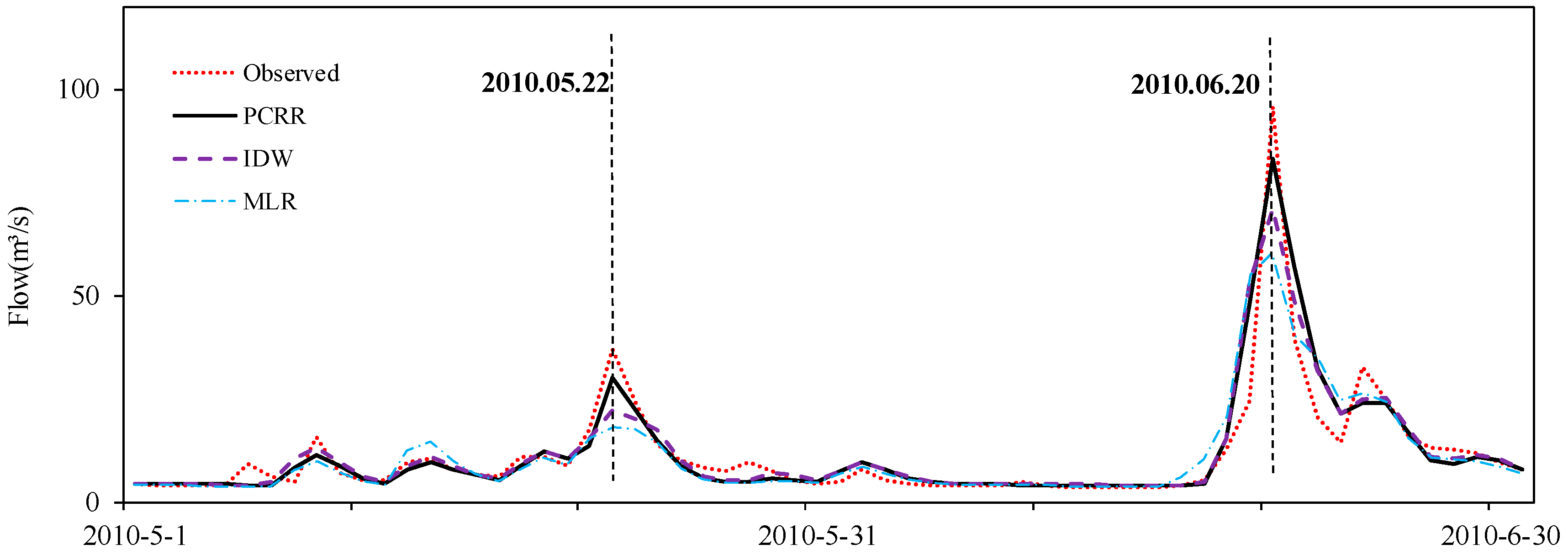
The differences between the interpolation methods were more pronounced over short time scales [10]. Monthly rainfall differences between the PCRR and IDW schemes ranged from −20 mm to +40 mm, and those between the PCRR and MLR methods ranged from −60 mm to +80 (Figure 5). These monthly differences generally exhibited maximum values between May and July. Thus, a visual analysis of the differences in runoff is shown in Figure 6 from May to June 2010. The peaks generally occurred at the same time in both model runs. 20 June 2010 was the peak runoff time of the entire period, and the measured peak discharge was 95.7 m³/s. The peak discharges determined using the three interpolation methods were lower than the measured values. The PCRR method yielded the closest estimate (83.2 m³/s), while the IDW and MLR values were 71 m³/s and 65.4 m³/s, respectively. A similar trend was observed for runoff processes on 22 May 2010. Figure 5 and Figure 6 reveal that, in general, large rainfall differences led to large peak flows, and the simulated streamflow volumes varied with the different inputs.

Further results of analysis, including important flow characteristics such as the annual mean flow, maximum and minimum annual mean flow, maximum and minimum daily flow, and upper 10th percentile flow, are shown in

Table 7. Comparisons of flow characteristics.

Flow Characteristics	Obs. (cm)	PCRR (cm)	IDW (cm)	MLR (cm)
Max. annual mean flow	152.1	156.9	162.2	147.5
Min. annual mean flow	53.9	57.1	60.4	56.9
Upper 10 percentile	212.6	189.7	209.4	202.8
Minimum daily flow	13.1	13.1	9.8	6.5
Maximum daily flow	3130.7	2489.5	2083.9	2460.1

. The values in bold were closest to the observed values. Generally, the flow characteristics obtained using the PCRR method were more similar to the observed data than those obtained using other methods, and daily streamflow characteristics exhibited large ranges between different simulations and flow characteristics.

3.3. Hourly Analysis

To further understand the performance of the interpolation methods and the objective verification based on streamflow simulations, investigations were performed for two flood events in the period between 2007 and 2013. Half-hourly precipitation was spatially interpolated using the three methods, and the results were used as input data in the HEC-HMS model. The selected events and important statistics are listed in

Table 8. Precipitation statistics of the selected events with hourly time step data.

Event	Period	Duration (h)	Average Rainfall Sum (mm/ev.)	Maximum (mm/h)	Average Rainfall Intensity (mm/h)
20100619	19 July–22 July 2010	69.5	160.3	14.8	2.3
20120430	30 April–3 May 2012	65.0	47.2	19.0	0.7

. The cross-validation performance (

Table 9. Cross-validation performance and ranking of different interpolation schemes for simulating flood events precipitation.

Interpolation Scheme	20100619			20120430
	PCRR	MLR	IDW	PCRR	MLR	IDW
Mean RMSE	0.712	1.74	0.83	0.42	0.96	0.44
Rank of mean RMSE	1	3	2	1	3	2
Mean MAE	0.52	0.71	0.65	0.32	0.72	0.23
Rank of mean MAE	1	3	2	2	3	1
MRE	1.07	2.1	1.39	7.06	9.54	2.25
Rank of mean MRE	1	3	2	2	3	1

) exhibited differences on the annual and daily scales. As shown in Table 8 and Table 9, of the three methods, the MLR method displayed the worst performance. However, there was little difference between the PCRR and IDW methods. The PCRR method exhibited a better interpolation effect for the No. 20100619 flood event, while the IDW method displayed better results for the No. 20120430 flood. In addition, the MRE method was significantly different compared with PCRR and MLR.

As with the daily model, the results of the three interpolation models were used as precipitation inputs for the HEC-HMS model, and the spatial distribution of the runoff results was obtained for different methods.

Table 10. Model performance of flood events using differently interpolated rainfall inputs.

Flood Event		20100619			20120430
		PCRR	IDW	MLR	PCRR	IDW	MLR
Runoff	Measured (mm)	141.7	141.7	141.7	53.6	53.6	53.6
	Simulated (mm)	148.7	127.6	144.1	46.7	49.8	31.5
	Relative Error (%)	4.95	−9.97	1.72	−12.82	−7.02	−41.24
Peak Discharge	Measured (m3/s)	166	166	166	74.7	74.7	74.7
	Simulated (m3/s)	160	145	188	82.2	76.3	83.6
	Relative Error (%)	−3.73	−12.47	13.19	10.04	2.14	11.91
Peak Time	Absolute Error (h)	2	2	1.5	1.00	1.00	1.00
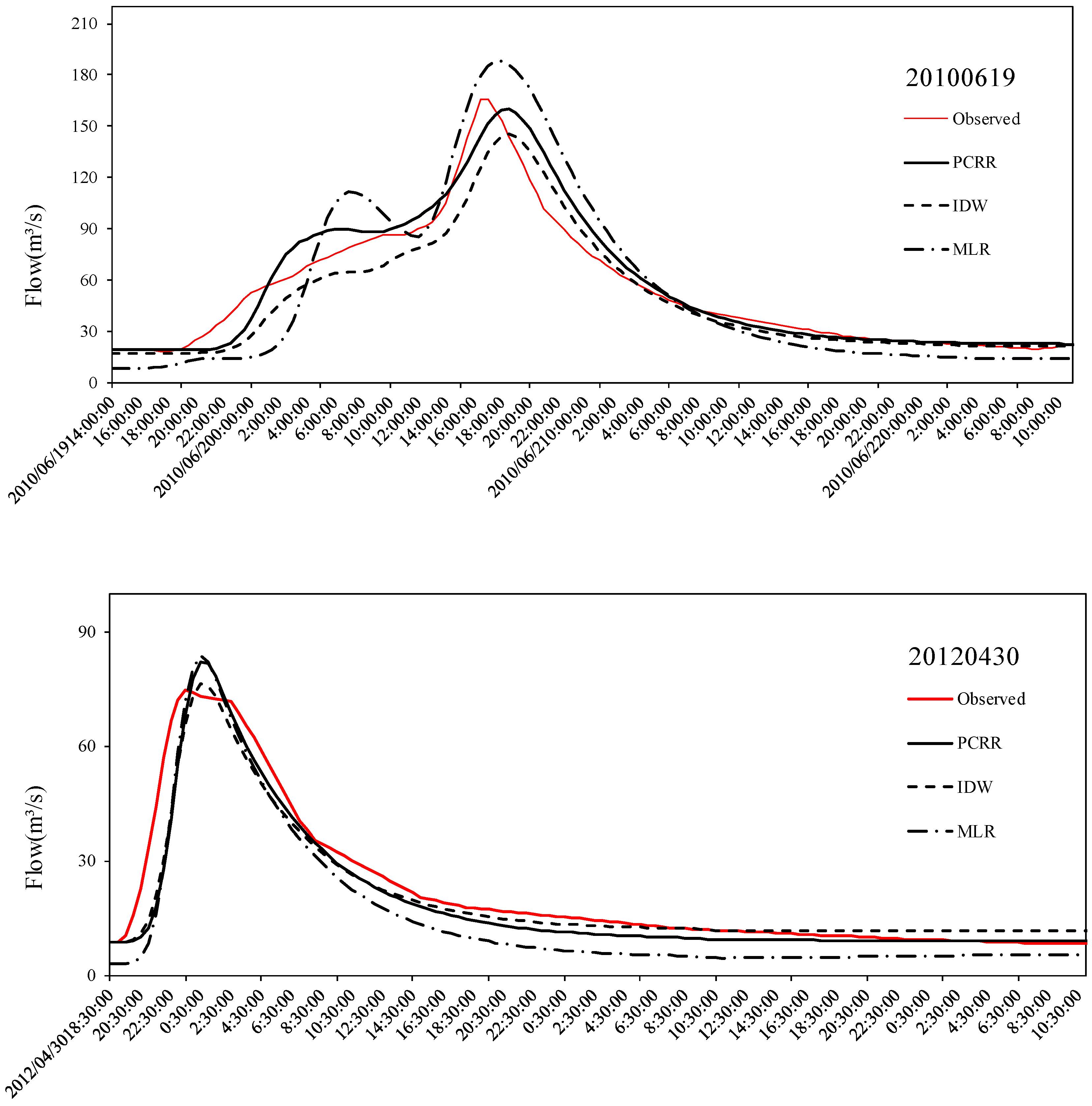
Nash–Sutcliffe efficiency		0.925	0.9	0.705	0.908	0.918	0.808

shows the statistical results of the two floods, which suggested that the results of the No. 20100619 flood using the PCRR method were slightly better than the results of the other two floods. However, for the No. 20120430 flood, the IDW method yielded the best results, which was consistent with the conclusion of cross-validation. A visual analysis of the differences in runoff is shown in Figure 7. For the No. 20100619 flood, all three methods yielded a distinct small peak before the flood peak, but the hydrograph of the measured discharge was not obvious, and this mismatch may be due to possible data error. The results of the three methods showed similar variations during the two flood events, and peak discharge was slightly larger than the measured discharge. Additionally, the flood peak time was about 1 h later than the measured peak time.

For the two flood events selected in this study, the differences between the hourly interpolation results of the three interpolation methods were not obvious, which is in agreement with Verworn’s conclusion [37]. Over a short time-series, heavy rain is concentrated as well as no precipitation for the rest time, which may lead to similar interpolation results. The distributions of runoff processes in the HEC-HMS model driven by PCRR and IDW were nearly identical, while that of the MLR method was quite different from the former two. This result also suggests that even slight differences in precipitation can cause dramatic differences in simulated streamflow.

4. Discussion

When using the hydrological model to reflect the difference of precipitation, a worthwhile discussion topic is that the ability to correctly reproduce surface runoff strictly depends on the rainfall-runoff transformation and the successful generation might not guarantee the correct reproduction of the precipitation field [38,39]. However, this study focuses on the comparison of interpolation methods. The traditional cross-validation method is often used for verifying the results. On the other hand, we also want to reflect the temporal and spatial distribution of precipitation interpolation from the side by means of the flow simulated by the hydrological model. Usually, this method is especially relevant in catchments that are dominated by heavy rainfall events, producing mostly direct runoff and resulting in highly dynamic hydrographs, which allow for a simple evaluation of rainfall inputs (Wagner et al. [18]).

Another discussion in this study is the selection of the hydrological model, which is also related to the correct reproduction of the precipitation field. In this study we used a semi-distributed hydrological model, which divides the study basin, an area of 96.4 km², into six sub-basins; each sub-basin can represent the internal spatial distribution. The area precipitation of each sub-basin is the average of the internal grids, which can reflect the geographical features of the catchment, so it can represent the spatial precipitation distribution information within the sub-basin. This can effectively explore the performance of the spatial precipitation interpolation method. Haberlandt et al. [33], Ruelland et al. [21], Masih et al. [40], Tobin et al. [41], and others also used semi-distributed hydrological modeling for the validation of interpolation methods. In addition, the HEC model has the characteristics of easy operation, short running time, the combination of a variety of multiple runoff-convergence schemes, and so on. At the same time, the study catchment is located in Jiangxi Province, where flash floods happened frequently; previous studies have used the HEC-HMS model (Li [42]; Wu et al. [43]) with good applicability. This model and parameter calibration procedure have been successfully applied in our previous study, ‘Flash Flood Forecasting and Disaster Management of Jiangxi Province’ (grant No. 0628-156104104417) project. Therefore, the semi-distributed HEC-HMS model was chosen.

HEC-HMS was used to evaluate runoff and describe the temporal and spatial distributions of rainfall. In this study, the genetic algorithm was used to automatically calibrate the model parameters to determine the maximum certainty coefficient as the objective function.

The results of cross-validation showed that the average annual rainfall value at each site simulated by the PCRR method was close to the measured value, while the IDW method yielded a negative trend at Yunfeng station. This negative trend is potentially important because the annual precipitation at Yunfeng station is 1970.4 mm, which is the largest among all gauges, and the elevation is the highest (341 m) among the gauges located within the basin. The precipitation predicted at all stations by the MLR method was less than the measured precipitation, reflecting a negative correlation. This negative correlation exists because the annual precipitation at all stations in the Xinxie catchment is greater than 1800 mm, while only seven of the 34 sites outside the basin have an annual precipitation greater than 1800 mm. It is worth mentioning that, because of this reason, the three methods used to predict annual precipitation values over 1800 mm yielded negative correlations. Since the PCRR residuals were further interpolated, the degree of negative correlation was the smallest among the three methods. Further research is needed to explore the generality of this result by using other models and other catchments.

Remarkably, although the results of MLR in cross-validation were only slightly worse than those of the other two methods, the hydrological response in the catchment associated with different interpolation methods can reflect a large difference. Hwang et al. [44] summarized the same conclusions in their study of spatial interpolation schemes of daily precipitation for hydrologic modeling. For the No. 20100619 flood, as shown in Figure 7, the MLR method produced a significant flood peak on June 20 from 04:00 to 10:00, while this peak was not obvious in the measured flow during this event. Compared with the measured peak flow, the MLR-based flow corresponded to a larger peak discharge and a longer duration, while the other two methods yielded flows that were slightly smaller than the observed peak discharge. For the No. 20120430 flood, the MLR method and PCRR method yielded the same peak flow, but the values of flood initiation and termination processes based on the MLR method were smaller than the measured values of those processes, resulting in relatively large error in the runoff depth.

Some limitations of this study are as follows. Only one small catchment, Xinxie, was chosen as the study area; this catchment is dominated by a tropical humid monsoon climate, and the terrain transitions from high to low from south to north. A distributed hydrological model will be introduced to compare the results with the HEC-HMS model and to study the spatial response between precipitation and runoff. Moreover, only two flood events were selected for hourly scale interpolation, and the small number of samples may not effectively reflect the effect of hourly scale interpolation schemes. Future studies will be conducted for a more comprehensive analysis.

5. Conclusions

In this study, three interpolation schemes were used to provide rainfall data on annual, daily, and hourly scales using seven rain gauges in the Xinxie catchment and 34 rain gauges surrounding the catchment as auxiliary sites. Cross-validation was used to evaluate different methods, and the HEC-HMS hydrological model was used to assess the performance of spatial integration.

Based on collinearity diagnosis, it can be concluded that there is strong collinearity in the MLR model, which will influence the least square estimation; however, this problem will not occur using the PCRR method. Our analysis shows that PCR based on the residual method, which involves elevation, slope, and slope aspect, performs the best on the annual and daily scales and shows little difference at the hourly scale compared to the results of the IDW method.

At the annual scale, the predicted value was slightly larger than the measured value when the annual precipitation was less than 1800 mm, reflecting a trend of overestimation. However, the predicted value was less than the measured value when the annual precipitation was more than 1800 mm, reflecting a trend of underestimation. At the daily scale, the differences between the indicators of the different methods increased obviously compared to those at the annual scale due to the increase in the spatial heterogeneity of precipitation at the daily scale. The cross-validation performances of different interpolation schemes differed at the hourly scale compared with those at the annual and daily scales. At the hourly scale, the PCRR and IDW methods performed better than the MLR method, but the difference between PCRR and IDW was not obvious.

Furthermore, to assess the accuracies of interpolated spatial distributions, a hydrological model was used to temporally and spatially integrate rainfall and simulate streamflow. Overall, large rainfall differences led to high differences in peak flows. The hydrological model driven by PCRR from 2007 to 2013 displayed good results, which suggested that the indicators of daily runoff processes were relatively accurate. Additionally, although the NSE of the IDW method was slightly less than that of the PCRR method, differences existed between various flow characteristics, such as the daily maximum flow and runoff depth. The three methods produced roughly the same simulation results for the two flood events, especially the No. 20120430 flood. The results showed that the peak discharge was greater than the observed discharge, and the simulated peak time was an hour later than the observed peak time.

In general, our results indicate the potential of using the PCRR method for rainfall interpolation. Moreover, different time scales can be used to more comprehensively assess model performance, and the use of hydrological models can be a complementary indicator of the quality of rainfall interpolation.