Article

Summer Season Water Temperature Modeling under the Climate Change: Case Study for Fourchue River, Quebec, Canada

1
Forecast and Control Division, Nakdong River Flood Control Office, Busan 49300, Korea
2
INRS-ETE, 490 rue de la Couronne, Québec, QC G1K 9A9, Canada
3
Department of Hydro Science and Engineering, Korea Institute of Civil Engineering and Building Technology, Goyang-si 10223, Gyeonggi-do, Korea
*
Author to whom correspondence should be addressed.
Water 2017, 9(5), 346; https://doi.org/10.3390/w9050346
Submission received: 2 November 2016 / Revised: 8 May 2017 / Accepted: 10 May 2017 / Published: 14 May 2017
(This article belongs to the Special Issue Ecological Responses of Lakes to Climate Change)

Abstract

:
It is accepted that human-induced climate change is unavoidable and it will have effects on physical, chemical, and biological properties of aquatic habitats. This will be especially important for cold water fishes such as trout. The objective of this study is to simulate water temperature for future periods under the climate change situations. Future water temperature in the Fourchue River (St-Alexandre-de-Kamouraska, QC, Canada) were simulated by the CEQUEAU hydrological and water temperature model, using meteorological inputs from the Coupled Model Intercomparison Project Phase 5 (CMIP5) Global Circulation Models (GCMs) with Representative Concentration Pathway (RCP) 2.6, 4.5 and 8.5 climate change scenarios. The result of the study indicated that water temperature in June will increase 0.2–0.7 °C and that in September, median water temperature could decrease by 0.2–1.1 °C. The rise in summer water temperature may be favorable to brook trout (Salvelinus fontinalis) growth, but several days over the Upper Incipient Lethal Temperature (UILT) are also likely to occur. Therefore, flow regulation procedures, including cold water releases from the Morin dam may have to be considered for the Fourchue River.

1. Introduction

Water temperature is one of the most important factors for physical, chemical, and biological properties of aquatic habitats [1,2,3], fish growth [4], spawning rate [5,6], and water quality [7,8]. In addition, it is especially important to cold water fishes such as salmonids [9,10,11,12,13,14]. Water temperature increases that could potentially be induced because of climate change could be a critical issue of aquatic species [15,16,17,18,19]. For instance, results of Bouck et al. [14] indicate that sustained water temperature over 24.0 °C can be lethal for certain species of salmonids.
A number of studies have been conducted on the analysis and simulation of water temperature under climate change. These studies can be divided into several topics: freshwater [18,20,21], saltwater [22,23,24], river [20,25,26], lake [27,28], ocean [29,30], global scale [21], etc. Furthermore, recent studies also have discussed water temperature change and its effect due to climate change on the aquatic environment such as ecosystem productivity [31,32] and biodiversity [24,33,34]. In particular, cold water species are studied more extensively because several climate change scenarios indicate that some rivers may approach their upper tolerance limit [35,36,37]. For instance, Johnson and Almlöf [34] discussed the potential impact of temperature increases on the brook trout population in one of Lake Superior’s tributary and Brown [24] shows the change in the exceedance of upper water temperature criteria, based on the climate change scenarios. Hence, water temperature issues could be one of the main challenges in the perspective of climate change and aquatic ecosystem.
The objective of this study is therefore to simulated future water temperature of the Fourchue River, which is a relatively small regulated river, using Coupled Model Intercomparison Project Phase 5 (hereafter referred to as CMIP5) global circulation models (hereafter referred to as GCMs) and Representative Concentration Pathway (hereafter referred to as RCP) 2.6, 4.5 and 8.5 climate change scenarios [38]. The CEQUEAU model was employed to simulate flows and water temperatures with future projected meteorological data. The Fourchue River has been previously studied by [39,40]. Beaupré [39] compared a deterministic [41] and a geostatistical [42] model. Kwak et al. [40] compared a deterministic [43] and two stochastic models [44,45] to estimate water temperatures in the river. For this follow-up study of [40], hydro-climatic data from 2011 to 2014 and future projected meteorological scenarios were obtained and used to simulate for future water temperature.

2. Study Area and Data

2.1. Study Area and Observed Data

The Fourchue River is the target basin, which has 261 km2 of area and is a tributary of the Du-Loup River in the eastern Quebec (QC, Canada), regulated by the Morin Dam, which has 38,880,000 m3 holding capacity and 680 ha reservoir area. The basin is mainly covered by forest and the river flows vary between 0.06 to 8.0 m3/s (Centre d’expertise hydrique Quebec). The water temperature of the Fourchue River was monitored during the summer seasons (June to September) from 2011 to 2014 with Hobo Pro V2 thermographs (±0.2 °C) sampling at 15 min interval. The water temperature loggers were deployed over an 8 km river reach, from directly downstream of the Morin dam to its confluence with the Du-Loup River. Air temperature was obtained from the Fourchue River meteorological station (Environment Canada; http://climate.weather.gc.ca), and the water level records of Morin dam were also collected. In addition, hydro-physiographic properties of the Fourchue River basin, required to run the deterministic model, were extracted from 3 km × 3 km grid DEM and land-use map (http://srtm.csi.cgiar.org/) (Figure 1).

2.2. Climate Change Projection

The World Climate Research Program (WCRP; http://www.wcrp-climate.org) develops global climate projections through its Coupled Model Inter-comparison Project (CMIP; http://www-pcmdi.llnl.gov) roughly every 5–7 years. To simulate water temperature in the Fourchue River under climate change condition, the CMIP5, the most recent of these simulations with a higher resolution [46], were obtained from the Pacific Climate Impacts Consortium of Canada (PCIC; http://www.pacificclimate.org/).

3. Methodology

3.1. Water Temperature Model: CEQUEAU Model

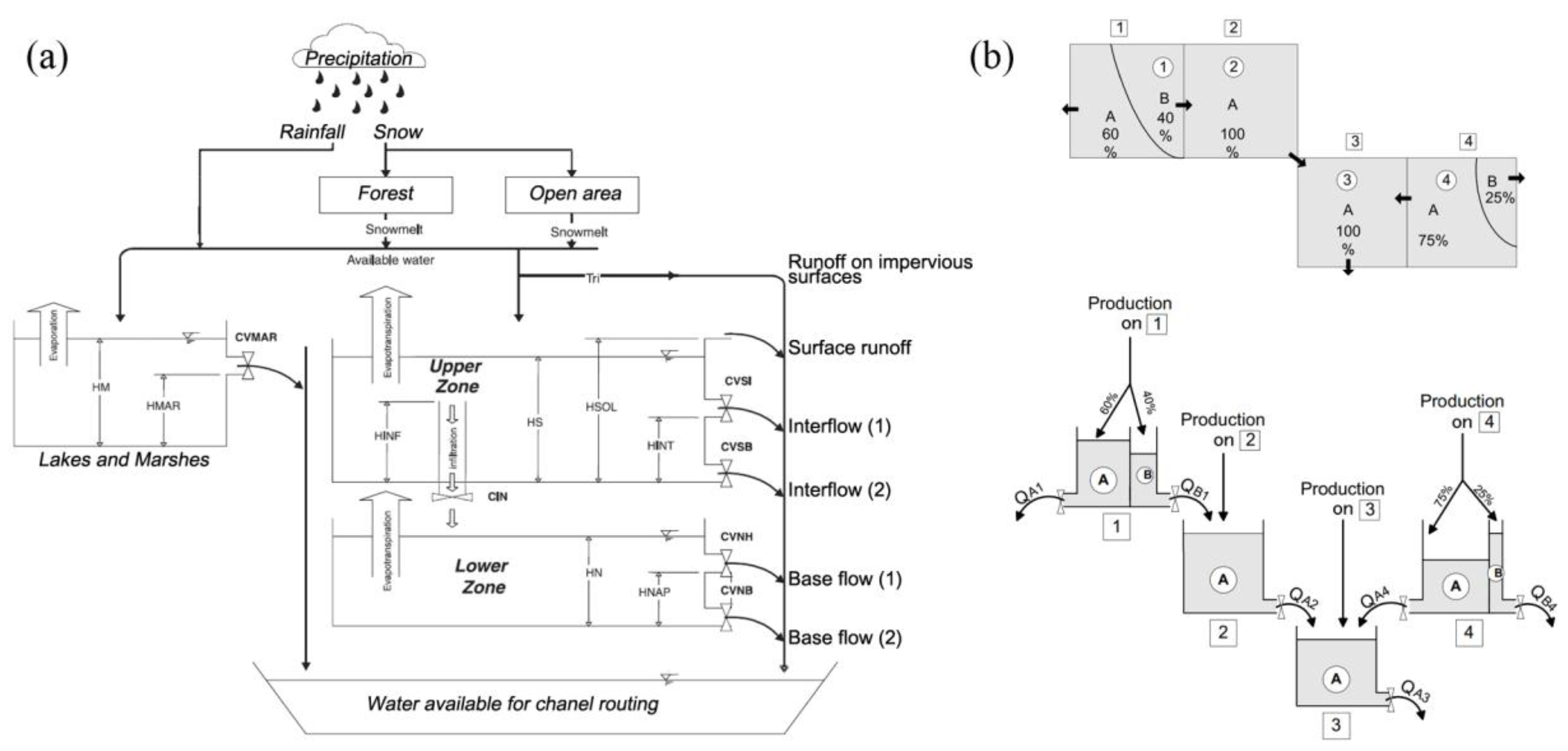
CEQUEAU is a hydrologic model that can simulate hydrological and thermal response with a hydrological heat budget module. It has shown good results in Canada [47,48], especially, it has produced relatively good flow and water temperature simulations for the Fourchue River [40], which is the study area. The CEQUEAU model is a semi-distributed hydrologic model which takes into account the hydro-physiographic characteristics of the basin [49]. As shown in Figure 1, the drainage basin is divided into hydrological units of equal size, called “whole squares”. Water Routing is based on the digital elevation model and the water divide in each square. For each whole square, a water balance calculation is completed at each time step, which accounts for water input from precipitation and/or snowmelt and loss by evapotranspiration. Water storage in lakes and marshes and infiltration of water into the ground are also conceptualized in the model by connected reservoirs (Figure 2). Subsequent runoff generation is thus calculated for each square of hydrological unit [43]. The CEQUEAU model comprises two functions to describe the runoff mechanism and upstream-downstream routing, the production function represents the vertical water routing (Figure 2a) and the routing function is used to estimate the amount of water transiting to the outlet of the basin (Figure 2b).

3.2. Climate Change Projection: Climate Scenario and Model

This study employed CMIP5, because it includes more GCMs with generally higher spatial resolution enabling to address a wider variety of scientific questions [50]. The future climate projection data obtained from Statistically Downscaled Climate Scenarios in Pacific Climate Impacts Consortium of Canada (PCIC). PCIC provides two downscaling methods, which are optimized for the North American continent: Bias Correction Spatial Disaggregation (BCSD) [51] with monthly time scale and Bias Correction Constructed Analogs (BCCA) [52] with daily time scale. Daily scenarios downscaled with the latter approach were employed as inputs for daily flow and water temperature simulations.
In addition, the climate projections vary based on the external forcing factor, greenhouse gas emission scenarios and numerical models [53]. The Intergovernmental Panel on Climate Change (IPCC; http://www.ipcc.ch/) determined the concentration of greenhouse gases based on human impact on the atmosphere as RCP (Representative Concentration Pathways) scenarios [54]. Climate change scenarios in CMIP5 describe four possible climatic futures (RCP 2.6, 4.5, 6.0 and 8.5), all of which are considered possible depending on how much greenhouse gases will be emitted [55] and depending on the degree of carbon dioxide reduction (Table 1). The selection of these scenarios is one of the important factors in the assessment of climate change. However, there is no evaluation of what is the most suitable scenario or GCM for the Fourchue River basin. Combinations of RCP 2.6, 4.5 and 8.5 scenarios provide a range of possible results. In addition, there are many CMIP5 GCMs that employ numerical equations to simulate the general circulation of a planetary atmosphere or ocean and used for weather forecasting, understanding the climate and forecasting climate change [50,53]. Based on the result of [56], twelve models that provide simulations for Eastern Canada were employed for the study area (Table 2). Among them, nine models were employed for RCP 2.6 scenarios and twelve models were employed for RCP 4.5 and 8.5 scenarios. In total, 33 projected climate data were used to simulate water temperature until year 2096 in the Fourchue River. Three GCM (Inmcm4, HadGEM2-CC, ACCESS1-0) with RCP 2.6 scenarios were excluded due to the air temperature mismatch for the observation periods. Each GCM used in this study have spatial resolutions ranging from 110 km2 to 310 km2 (Table 2).

3.3. Quantile Mapping

Usually, GCM and regional climate model (hereafter referred to as RCM) are known to have systematic biases at local or basin scale [58]. Consequently, GCM and RCM projected data need post-processing to produce reliable estimations at local scale. The quantile mapping method was employed to remove biases between observed and projected data. The corrected variable is:
Z   =   C D F 1 o b s (   C D F s i m   ( X   ) )
where C D F o b s and C D F s i m are the cumulative distribution function of the observed and corresponding simulated daily value, respectively. This method has been widely used to correct bias at the basin scale due to its simplicity [59].

4. Result and Discussion

4.1. Water Temperature Modeling

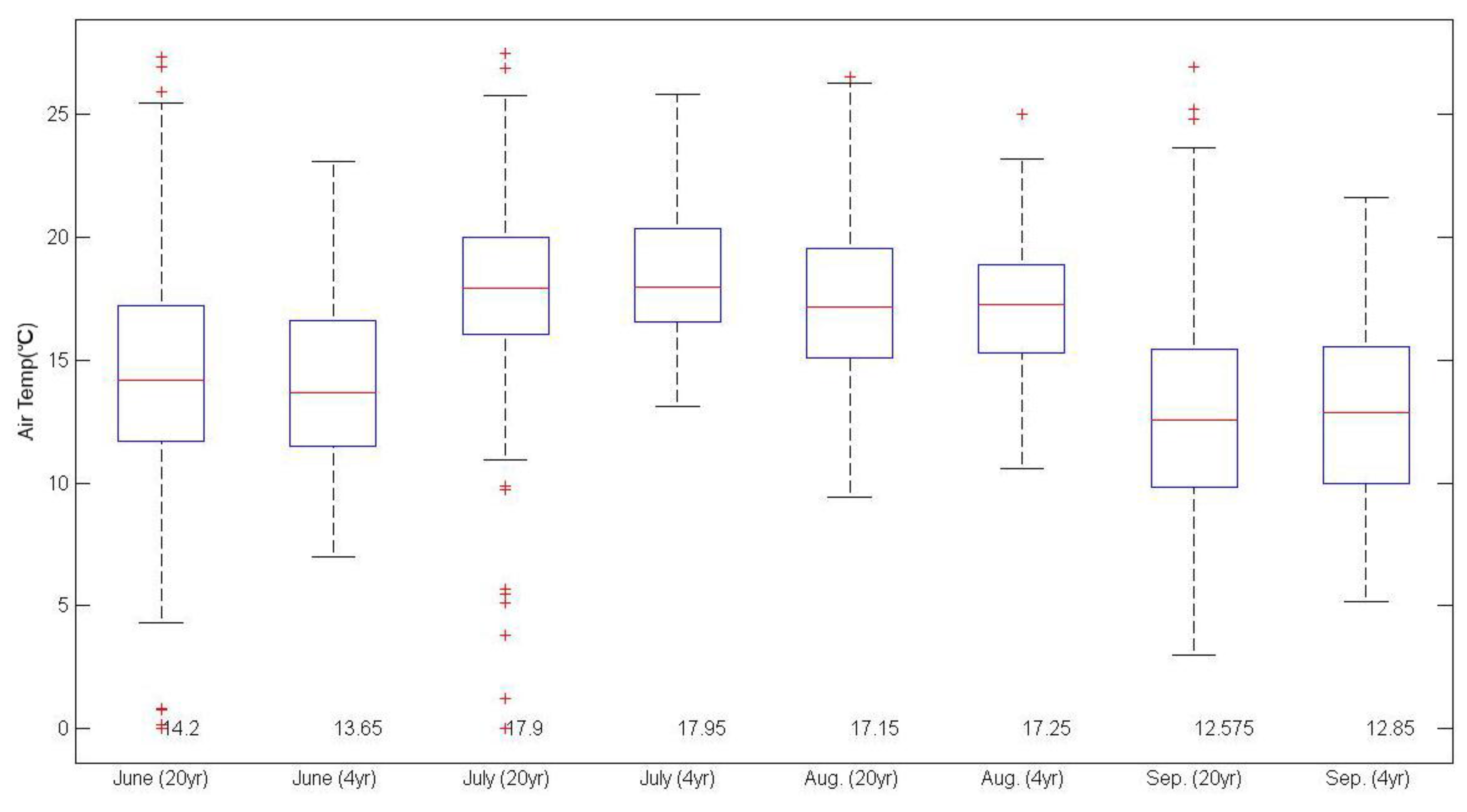
Relatively small water temperature time series is one of the limitations of this study, with only four years of water temperature data during summer season being available. The CEQUEAU model had to be calibrated and validated using this limited dataset. One concern is that the years of calibration be atypical and that the resulting calibration of the hydrologic/water temperature model be inadequate. Figure 3 shows daily air temperature boxplots of the last 20 years and the four years with water temperature observations and it shows that the last four years are a good representation of the longer climate time series, albeit with smaller variance.
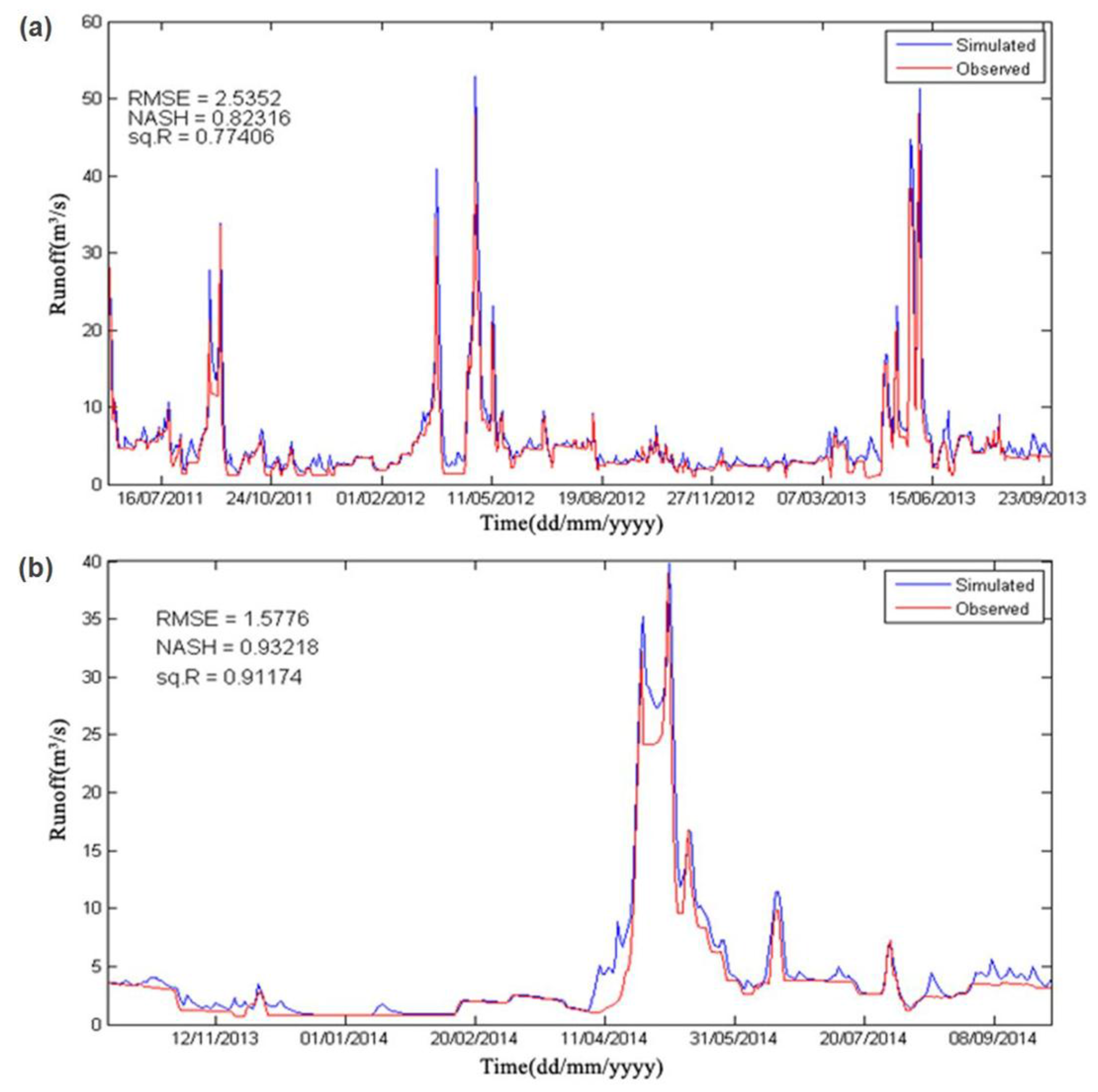
Model parameters were adjusted by hand using simulated vs. observed water level of the Morin dam and water temperature upstream and downstream of the dam using 2011 to 2013 data for calibration and 2014 data for validation. Flows were also used. Runoff at the Morin dam outlet was estimated using the reservoir storage-runoff curves developed for each month. Figure 4 shows the calibration and validation results, with simulated flows closely matching observed values and RMSE and R2 [60], Nash–Sutcliffe model efficiency coefficient [61] values of 2.54 m3/s, 0.77, and 0.82 for the calibration period and 1.58 m3/s, 0.91, and 0.93 for the validation period, respectively. The RMSEs is the average measure of error in the predictions, and R2 and Nash–Sutcliffe model efficiency coefficient describe the prediction efficiency of hydrological models [62]. Therefore, CEQUEAU models have the capacity to explain 78–90% of the variances in the calibration and validation periods, respectively. What is unique about calibration and validation result is that the calibration phase shows slightly poorer performance than validation. The cause of this discrepancy seems to be linked to greater flow variability in the calibration period (2012 to 2013) than during validation. The runoff time series in the validation has just one major runoff event in March 2014.
The temperature component of the CEQUEAU model computes a heat budget based on the volume of water modeled by the hydrological module of CEQUEAU. The sum of short wave solar radiation (+), net longwave radiation (±), latent heat (−), sensible heat (±), heat advection from upstream (±), heat loss downstream (−) and local contributions from groundwater and interflow (±) were considered at each time step in the heat budget terms.

4.2. Meteorological Predictor Estimation under Climate Change

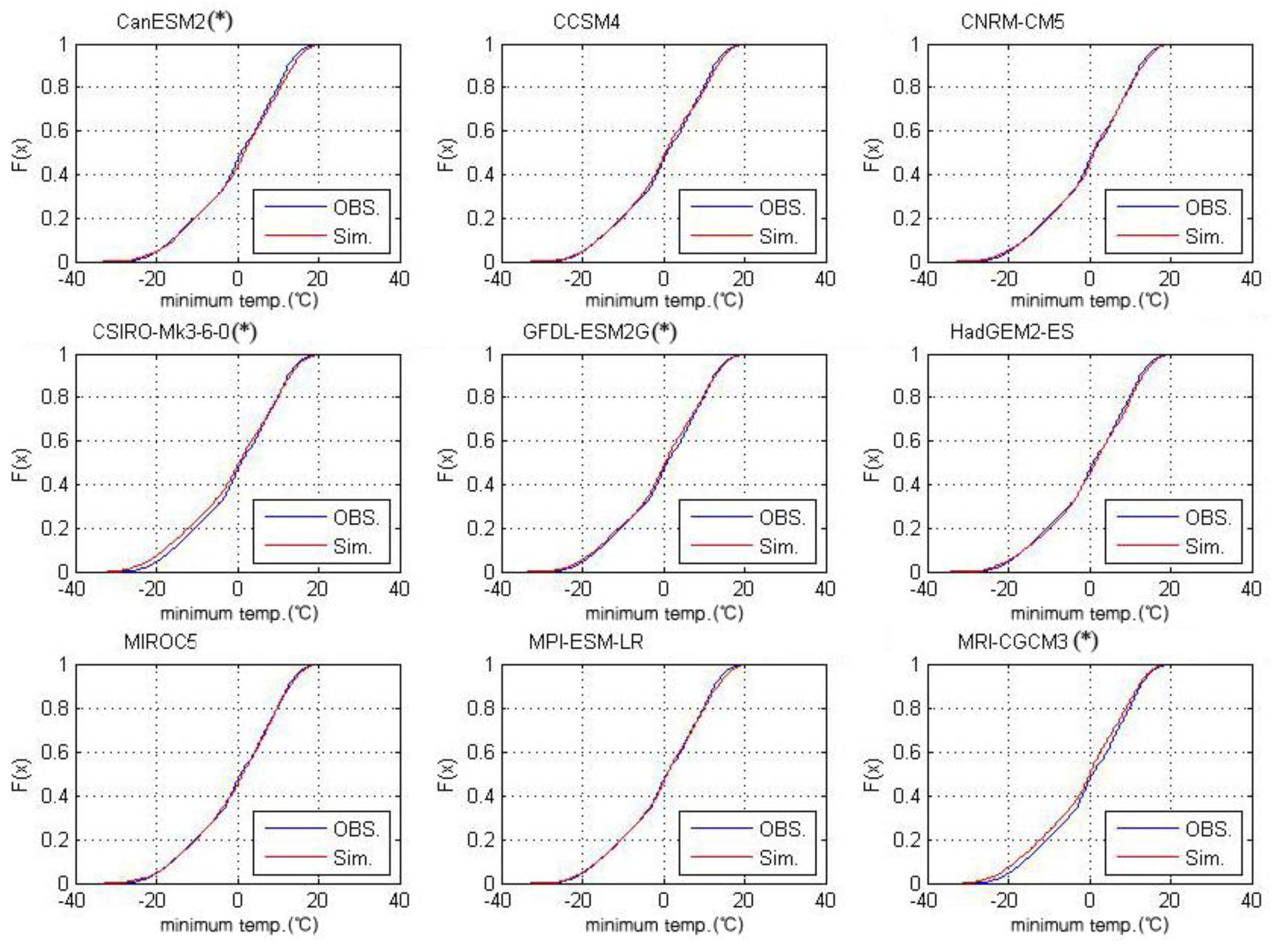
PCIC projection with RCP 2.6, 4.5, 8.5 and each GCM listed above provided the climate projections for this study. However, GCM and RCM are known to have systematic biases at local or basin scale [58], and PCIC could also be biased. This was checked using a Kolmogorov–Smirnov test [63] to compare the cumulative distributions of observed versus simulated air temperatures (Figure 6) and precipitations.
As the result of two-variable Kolmogorov–Smirnov test with 95% significance level between observed maximum, minimum, mean temperature, precipitation in projected and observed data for 1994–2014 (20 year), several climate model outputs were determined to have different distributions than observed for the recent past period (1994–2014 years). Quantile mapping technique was employed to correct the bias of climate models, when the test null hypothesis of identical distributions was not verified (see the Supplementary Figure S1).
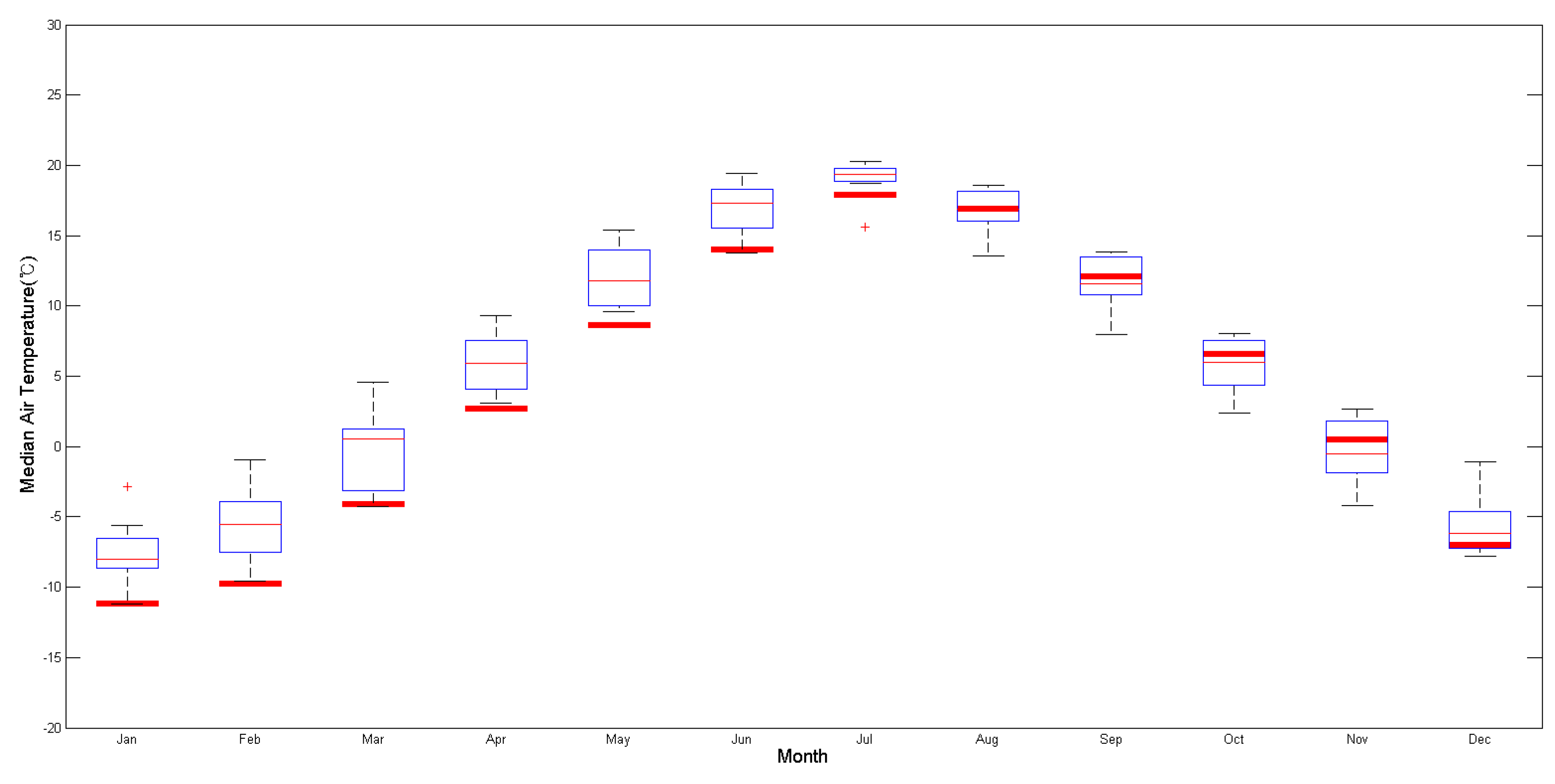
The Figure 7 shows the overall trend of monthly median air temperature from the projected climate data. It indicates that the seasonal water temperature signal of the Fourchue River could be shifted in the future. In detail, December to July shows warming trend of about 2.0 to 4.0°C, and August to November shows cooling trend of 0.5 to 1.0°C. Among these, potential increases in water temperature in the summer season can significantly affect cold water fish species such as salmonids, as indicated previously.

4.3. Future Water Temperature Simulation

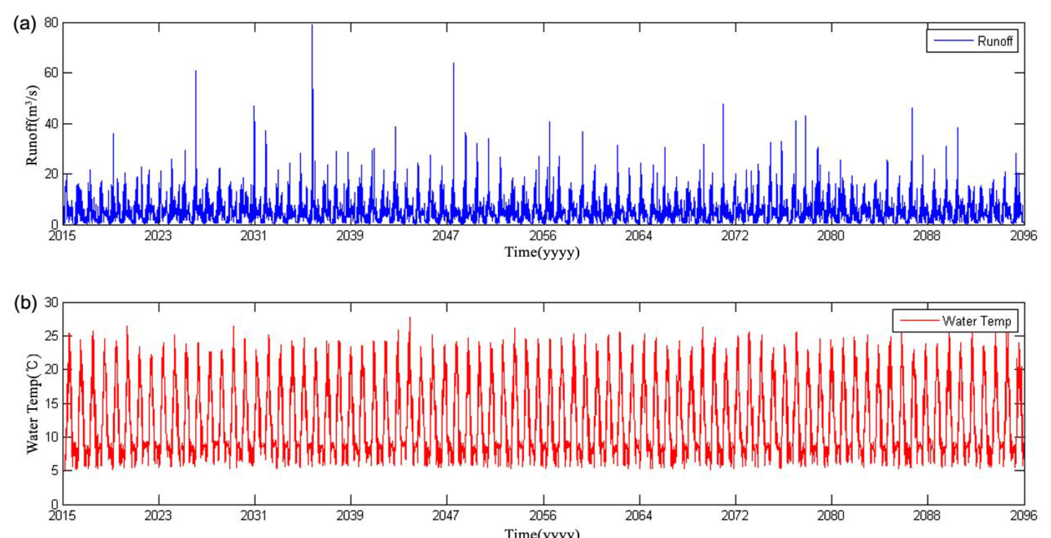
The study simulated the future runoff and water temperature in summer season using climate data from 2016 to 2096 according to RCP 2.6, 4.5 and 8.5 climate change scenarios and various climate models feeding inputs to the CEQUEAU model. In addition, weekly average discharge rate from Morin dam were estimated from observed records and used as the discharge data from the dam, and the CEQUEAU model parameters were adjusted to consider systematic negative bias due to Morin dam [40]. The simulated results are shown in Figure 8.
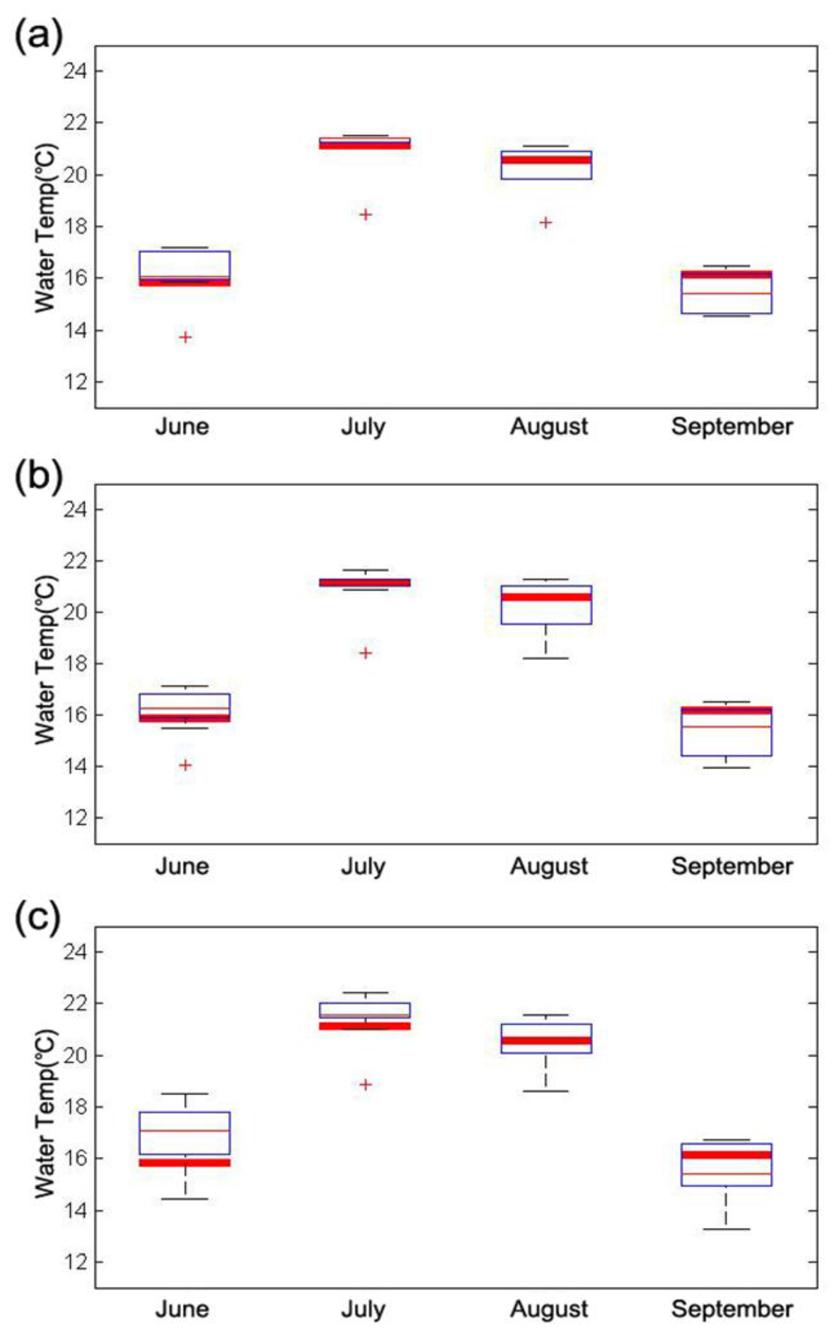
The water temperature of the summer season (June to September) is the main focus of this study. Boxplots of daily water temperature in the summer season of the Fourchue River for the years 2016 to 2096 show differences between scenarios (Figure 9).
IPCC suggested that Eastern Canada region will undergo an air temperature increase of 2–3 °C over the mid-term (2046–2065) and 4–5 °C on the long-term (2066–2100) according to the RCP 8.5 scenario, with the most warming in the northern portion, and the least warming in the southern region near the Atlantic Ocean [64]. The Fourchue River is located in the southeastern region, so it seems that it may be less affected by global warming than other regions in Canada. However, the projected temperatures show possible non-negligible changes, as shown by Figure 9 and Table 3. July and August show similar or slightly higher median value than the present, but there are relatively important projected changes in June and September (Table 3). In June, water temperature medians for the future scenarios are 16.04 (+0.2) °C in RCP 2.6, 16.03 (+0.2) °C in RCP 4.5 and 16.50 (+0.7) °C in RCP 8.5. In September, projected future monthly medians are lower than in the recent past: 15.96 (−0.2) °C in RCP 2.6, 15.45 (−0.7) °C in RCP 4.5 and 14.97 (−1.1) °C in RCP 8.5. According to the different scenarios, shifts are expected in June for the next decade (2016 to 2025), with median projected water temperature increasing by +0.2 °C in RCP 2.6, +0.4 °C in RCP 4.5 and +1.2 °C in RCP 8.5, compared to the recent past (Figure 9 and Table 3). It could be assumed that seasonal shift will occur in the Fourchue River basin, and also the heat budget and its balance in the basin will be change.
Considering Figure 7, the water temperature of the Fourchue River may also be subjected to a seasonal shift which can have repercussions on the aquatic ecosystems. Of course, these changes are relatively smaller than those projected for air temperature (Table 1 and [54]), but such changes could affect salmonid habitat. For instance, optimal temperature for growth of the brook trout (S. fontinalis), are between 14.4 and 16.0 °C [65]. The water temperature in June will have reached or exceeded the optimal growth temperature thereby affecting the growth rates for brook trout (Table 4).
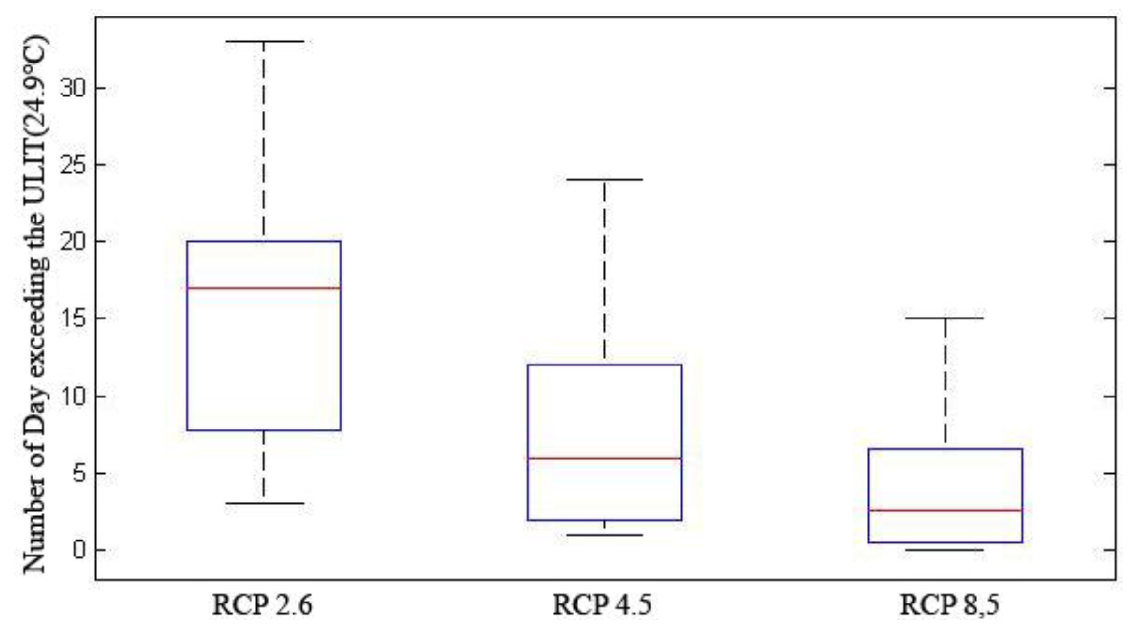
In addition, another concern is the upper incipient lethal temperature (UILT) which is the upper threshold for no mortality from temperature [68]. The UILT of the brook trout is approximately 24.9 °C [69]. In the observed period (2011 to 2014), this threshold was not exceeded, as the warmest daily water temperature is 24.44 °C on 5 August 2012. However, simulation result with each RCP scenario has several days over UILT (Figure 10).
In contrast with the comparison of median water temperature values, the median number of days over UILT is highest in RCP 2.6 (average of 17 days), and lowest for RCP 8.5 (average of three days). RCP 2.6, which is the most optimistic future scenario, has a relatively large number of days over UILT for brook trout, despite the fact that it has lower change in mean water temperature than RCP 8.5. Thus, the rise in air temperature, which is mainly responsible for the associated rise in water temperature [70], is increasing from RCP 2.6 to RCP 8.5 [64], but RCP 2.6 has more extreme events than RCP 4.5 and 8.5. Consequently, future water temperature in the Fourchue River may provide risk for Brook trout, as shown by the change of water temperature in summer season and UILT exceedances for all climate change scenarios. Moreover, these changes will affect to overall condition of the aquatic ecosystem, especially, median air temperature as indicated in Figure 7. The water temperature simulations shown in Figure 9 and Table 3 indicate a potentially high probability of seasonal shifts in the Fourchue River in the future, which could cause significant change in cold water species behavior and condition. Key components of the life cycle such as egg incubation and juvenile rearing could be impacted. Further studies are needed to face this challenge. Given that the Fourchue River in impounded, flow regulation procedures could be changed and cold water releases from the dam may have to be considered to maintain optimal temperatures and minimize the risk of UILT exceedances.
There are two limitations in this study, the one concern is the relatively small time series of four years (2011 to 2014) of water temperature data during summer season (June to September). It should be mentioned that there are very few water temperature monitoring sites on regulated rivers in Eastern Canada. In this context, having four years of data is actually a rarity. The other concern is the climate change projection because the projected future scenarios are a result from numerical models (GCMs), with potential bias an associated uncertainty. Especially, the seasonal shift, which seems to be occurred in the near future based on the PCIC and this study, will be the most important challenge, so it need further studies why or how it will occur. However, using model outputs are the most effective tool to simulate future water temperature scenarios and provide some insight on the impact of potential shifts of the thermal regime of rivers on aquatic habitat.

5. Conclusions

This study provided simulations of future water temperature scenarios of the Fourchue River, Quebec, QC, Canada, using CMIP5 climate model and RCP 2.6, 4.5 and 8.5 climate change scenarios. The median air temperature and the water temperature simulation results indicated that there is a relatively important probability of thermal seasonal shifts in the Fourchue River in the future. Should it materialize, it will cause significant habitat changes for cold water species. The main conclusions are:
(1)
As shown by the water temperature results of the CEQUEAU model simulations for the future period, it is possible that the median water temperature in June will increase 0.2–0.7 °C and that, in September, median water temperature could decrease by 0.2–1.1 °C, The rise in water temperature in June may be favorable to brook trout growth, as temperatures will be near or exceeding the optimal growth range (16.0 °C). However, several days over UILT (24.9 °C) for brook trout are also likely to occur, according to different scenarios.
(2)
The change of water temperature in summer season will affect the overall conditions of the aquatic ecosystem and its related environment and industries. Therefore, flow regulation procedures, including cold water releases from the Morin dam, may have to be considered to mitigate the negative effects of more extreme temperature occurrences on the Fourchue River.

Supplementary Materials

The following are available online at www.mdpi.com/2073-4441/9/5/346/s1, Figure S1: Quantile mapping results of maximum temperature for each month with CanESM2 and RCP 2.6 scenarios, Figure S2. Boxplot of monthly median air temperature from 2020 to 2096 years for RCP 2.6 with 9 climate models; bold red line indicate monthly median temperature for observed period (2011 to 2014), Figure S3. Boxplot of monthly median air temperature from 2020 to 2096 years for RCP 4.5 with 12 climate models; bold red line indicate monthly median temperature for observed period (2011 to 2014).

Acknowledgments

This research was supported by a grant (MPSS-NH-2015-79) through the Disaster and Safety Management Institute funded by Ministry of Public Safety and Security of Korean government and the NSERC HYDRONET strategic network.

Author Contributions

This research was carried out in collaboration among all authors. André St-Hilaire and Fetah Chebana had the original idea and led the research; Jaewon Kwak and Gilho Kim performed the data processing and analysis; and Gilho Kim edited the final manuscript. All authors reviewed and approved the manuscript.

Conflicts of Interest

The authors declare no conflict of interest.

References

  1. Coutant, C.C. Perspective on Temperature in the Pacific Northwest’s Fresh Water (No. ORNL/TM-1999/44); Oak Ridge National Laboratory: Oak Ridge, TN, USA, 1999. [Google Scholar] [CrossRef]
  2. Nunn, A.D.; Cowx, I.G.; Frear, P.A.; Harvey, J.P. Is water temperature an adequate predictor of recruitment success in cyprinid fish populations in lowland rivers? Freshw. Biol. 2003, 48, 579–588. [Google Scholar] [CrossRef]
  3. Coulter, D.P. Consequences of Short-Term Water Temperature Variability to Fish: Current and Future Climate Change Impacts. Ph.D. Thesis, Purdue University, West Lafayette, IN, USA, 2015. [Google Scholar]
  4. Sloat, M.R.; Shepard, B.B.; White, R.G.; Carson, S. Influence of stream temperature on the spatial distribution of west slope cutthroat trout growth potential within the Madison river basin, Montana. N. Am. J. Fish. Manag. 2005, 25, 225–237. [Google Scholar] [CrossRef]
  5. Handeland, S.O.; Imsland, A.K.; Stefansson, S.O. The effect of temperature and fish size on growth, feed intake, food conversion efficiency and stomach evacuation rate of Atlantic salmon post-smolts. Aquaculture 2008, 283, 36–42. [Google Scholar] [CrossRef]
  6. Besson, M.; Vandeputte, M.; van Arendonk, J.A.M.; Aubin, J.; de Boer, I.J.M.; Quillet, E.; Komen, H. Influence of water temperature on the economic value of growth rate in fish farming: the case of sea bass (Dicentrarchus labrax) cage farming in the Mediterranean. Aquaculture 2016, 462, 47–55. [Google Scholar] [CrossRef]
  7. Shrestha, S.; Kazama, F. Assessment of surface water quality using multivariate statistical techniques: A case study of the Fuji river basin. Jpn. Environ. Model. Softw. 2007, 22, 464–475. [Google Scholar] [CrossRef]
  8. Chang, H. Spatial analysis of water quality trends in the Han river basin, South Korea. Water Res. 2008, 42, 3285–3304. [Google Scholar] [CrossRef] [PubMed]
  9. Goniea, T.M.; Keefer, M.L.; Bjornn, T.C.; Peery, C.A.; Bennett, D.H.; Stuehrenberg, L.C. Behavioral thermoregulation and slowed migration by adult fall chinook salmon in response to high Columbia river water temperatures. Trans. Am. Fish. Soc. 2006, 135, 408–419. [Google Scholar] [CrossRef]
  10. Isaak, D.J.; Luce, C.H.; Rieman, B.E.; Nagel, D.E.; Peterson, E.E.; Horan, D.L.; Parkes, S.; Chandler, G.L. Effects of climate change and wildfire on stream temperatures and salmonid thermal habitat in a mountain river network. Ecol. Appl. 2010, 20, 1350–1371. [Google Scholar] [CrossRef] [PubMed]
  11. Parra, I.; Almodóvar, A.; Ayllón, D.; Nicola, G.G.; Elvira, B. Unravelling the effects of water temperature and density dependence on the spatial variation of brown trout (Salmo trutta) body size. Can. J. Fish. Aquat. Sci. 2012, 69, 821–832. [Google Scholar] [CrossRef]
  12. Lahnsteiner, F. Thermotolerance of Brown Trout, Salmo Trutta, Gametes and embryos to increased water temperatures. J. Appl. Ichthyol. 2012, 28, 745–751. [Google Scholar] [CrossRef]
  13. Matthews, K. California Golden Trout: Can their warming streams handle other stressors? Procedings of the 144th Annual Meeting of the American Fisheries Society (AFS), Quebec, QC, Canada, 17–21 August 2014. [Google Scholar]
  14. Bouck, G.R.; Chapman, G.A.; Schneider, P.W.; Stevens, D.G. Effects of holding temperatures on reproductive development in adult sockeye salmon (Oncorhynchus Nerka). In Proceedings of the 26th Annual Northwest Fish Culture Conference, Centralia, WA, USA, 6–7 December 1975. [Google Scholar]
  15. Poff, N.L.; Brinson, M.M.; Day, J.W. Aquatic Ecosystems and Global Climate Change; Pew Center on Global Climate Change: Arlington, VA, USA, 2002. [Google Scholar]
  16. Reist, J.D.; Wrona, F.J.; Prowse, T.D.; Power, M.; Dempson, J.B.; Beamish, R.J.; Sawatzky, C.D. General effects of climate change on arctic fishes and fish populations. AMBIO J. Hum. Environ. 2006, 35, 370–380. [Google Scholar] [CrossRef]
  17. Bärlocher, F.; Seena, S.; Wilson, K.P.; Dudley Williams, D. Raised water temperature lowers diversity of hyporheic aquatic hyphomycetes. Freshw. Biol. 2008, 53, 368–379. [Google Scholar] [CrossRef]
  18. Wenger, S.J.; Isaak, D.J.; Luce, C.H.; Neville, H.M.; Fausch, K.D.; Dunham, J.B.; Dauwalter, D.C.; Young, M.K.; Elsner, M.M.; Rieman, B.E.; et al. Flow regime, temperature, and biotic interactions drive differential declines of trout species under climate change. Proc. Natl. Acad. Sci. USA 2011, 108, 14175–14180. [Google Scholar] [CrossRef] [PubMed]
  19. Trumpickas, J.; Shuter, B.J.; Minns, C.K.; Cyr, H. Characterizing patterns of nearshore water temperature variation in the North American Great Lakes and assessing sensitivities to climate change. J. Gt. Lakes Res. 2015, 41, 53–64. [Google Scholar] [CrossRef]
  20. Kaushal, S.S.; Likens, G.E.; Jaworski, N.A.; Pace, M.L.; Sides, A.M.; Seekell, D.; Belt, K.T.; Secor, D.H.; Wingate, R.L. Rising stream and river temperatures in the United States. Front. Ecol. Environ. 2010, 8, 461–466. [Google Scholar] [CrossRef]
  21. Van Vliet, M.T.; Franssen, W.H.; Yearsley, J.R.; Ludwig, F.; Haddeland, I.; Lettenmaier, D.P.; Kabat, P. Global river discharge and water temperature under climate change. Glob. Environ. Chang. 2013, 23, 450–464. [Google Scholar] [CrossRef]
  22. Hunt, G.L.; Stabeno, P.J. Climate change and the control of energy flow in the southeastern Bering Sea. Prog. Oceanogr. 2002, 55, 5–22. [Google Scholar] [CrossRef]
  23. Gille, S.T. Decadal-scale temperature trends in the Southern Hemisphere Ocean. J. Clim. 2008, 21, 4749–4765. [Google Scholar] [CrossRef]
  24. Brown, A. Biodiversity: Stream temperature velocity. Nat. Clim. Chang. 2016, 6, 440. [Google Scholar] [CrossRef]
  25. Morrison, J.; Quick, M.C.; Foreman, M.G. Climate change in the Fraser River watershed: Flow and temperature projections. J. Hydrol. 2002, 263, 230–244. [Google Scholar] [CrossRef]
  26. Ferrari, M.R.; Miller, J.R.; Russell, G.L. Modeling changes in summer temperature of the Fraser River during the next century. J. Hydrol. 2007, 342, 336–346. [Google Scholar] [CrossRef]
  27. Fang, X.; Stefan, H.G. Projections of climate change effects on water temperature characteristics of small lakes in the contiguous US. Clim. Chang. 1999, 42, 377–412. [Google Scholar] [CrossRef]
  28. Quayle, W.C.; Peck, L.S.; Peat, H.; Ellis-Evans, J.C.; Harrigan, P.R. Extreme responses to climate change in Antarctic lakes. Science 2002, 295, 645. [Google Scholar] [CrossRef] [PubMed]
  29. Mann, M.E.; Zhang, Z.; Hughes, M.K.; Bradley, R.S.; Miller, S.K.; Rutherford, S.; Ni, F. Proxy-based reconstructions of hemispheric and global surface temperature variations over the past two millennia. Proc. Natl. Acad. Sci. USA 2008, 105, 13252–13257. [Google Scholar] [CrossRef] [PubMed]
  30. Hansen, J.; Ruedy, R.; Sato, M.; Lo, K. Global surface temperature change. Rev. Geophys. 2010, 48, RG4004. [Google Scholar] [CrossRef]
  31. Islam, M.N.; Bhuyain, M.A.B.; Mannan, M.A.; Hossain, M.I.; Ali, M.L. Study on environmental implications and its impact on aquatic productivity in the Southwest coastal region. J. Environ. Sci. Nat. Resour. 2015, 6, 71–78. [Google Scholar] [CrossRef]
  32. Munroe, D.M.; Narváez, D.A.; Hennen, D.; Jacobson, L.; Mann, R.; Hofmann, E.E.; Klinck, J.M. Fishing and bottom water temperature as drivers of change in maximum shell length in Atlantic surfclams (Spisula solidissima). Estuar. Coast. Shelf Sci. 2016, 170, 112–122. [Google Scholar] [CrossRef]
  33. Thompson, P.L.; Shurin, J.B. Regional zooplankton biodiversity provides limited buffering of pond ecosystems against climate change. J. Anim. Ecol. 2012, 81, 251–259. [Google Scholar] [CrossRef] [PubMed]
  34. Johnson, R.K.; Almlöf, K. Adapting boreal streams to climate change: effects of riparian vegetation on water temperature and biological assemblages. Freshw. Sci. 2016, 35, 984–997. [Google Scholar] [CrossRef]
  35. Santiago, J.M.; García de Jalón, D.; Alonso, C.; Solana, J.; Ribalaygua, J.; Pórtoles, J.; Monjo, R. Brown trout thermal niche and climate change: Expected changes in the distribution of cold-water fish in central Spain. Ecohydrology 2015, 9, 514–528. [Google Scholar] [CrossRef]
  36. Selbig, W.R. Simulating the effect of climate change on stream temperature in the Trout Lake Watershed, Wisconsin. Sci. Total Environ. 2015, 521, 11–18. [Google Scholar] [CrossRef] [PubMed]
  37. Al-Chokhachy, R.; Schmetterling, D.A.; Clancy, C.; Saffel, P.; Kovach, R.P.; Nyce, L.G.; Pierce, R. Are brown trout replacing or displacing bull trout populations in a changing climate? Can. J. Fish. Aquat. Sci. 2016, 73, 1395–1404. [Google Scholar] [CrossRef]
  38. Moss, R.; Babiker, M.; Brinkman, S.; Calvo, E.; Carter, T.R.; Edmonds, J.; Elgizouli, I.; Emori, S.; Erda, L.; Hibbard, K.; et al. Towards New Scenarios for Analysis of Emissions, Climate Change, Impacts, and Response Strategies: IPCC Expert Meeting Report; IPCC Secretariat: Geneva, Switzerland, 2008. [Google Scholar]
  39. Beaupré, L. Comparaison de Modèles Thermiques Statistique et Déterministe Pour L’estimation D’indices Thermiques sur les Portions Aménagées et Naturelles de la Rivière Fourchue. Master’s Thesis, INRS-ETE, Quebec, QC, Canada, 2014. [Google Scholar]
  40. Kwak, J.; St-Hilaire, A.; Chebana, F. A comparative study for water temperature modelling in a small basin, the Fourchue River, Quebec, Canada. Hydrol. Sci. J. 2016, 62, 64–75. [Google Scholar] [CrossRef]
  41. Bartholow, J.M. The Stream Network Temperature Model (SNTEMP): A Decade of Results. In Workshop on Computer Application in Water Management; GPAC Publication: Fort Collins, CO, USA, 1995. [Google Scholar]
  42. Guillemette, N.; St-Hilaire, A.; Ouarda, T.B.M.J.; Bergeron, N.; Robichaud, E.; Bilodeau, L. Feasibility study of a geostatistical model of monthly maximum stream temperatures in a multivariate space. J. Hydrol. 2009, 364, 1–12. [Google Scholar] [CrossRef]
  43. Morin, G.; Sochanski, W.; Paquet, P. Le mode`le de simulation de quantite´ CEQUEAU-ONU, Manuel de re´fe´rences. J. Vasc. Interv. Radiol. 1998, 22, S514. [Google Scholar]
  44. Diaconescu, E. The use of NARX neural networks to predict chaotic time series. WSEAS Trans. Comput. Res. 2008, 3, 182–191. [Google Scholar]
  45. Diversi, R.; Guidorzi, R.; Soverini, U. Identification of ARMAX models with noisy input and output. IFAC Proc. Vol. 2011, 18, 13121–13126. [Google Scholar] [CrossRef]
  46. Knutti, R.; Sedláček, J. Robustness and uncertainties in the new CMIP5 climate model projections. Nat. Clim. Chang. 2013, 3, 369–373. [Google Scholar] [CrossRef]
  47. St-Hilaire, A.; El-Jabi, N.; Caissie, D.; Morin, G. Sensitivity analysis of a deterministic water temperature model to forest canopy and soil temperature in Catamaran Brook (New Brunswick, Canada). Hydrol. Proc. 2003, 17, 2033–2047. [Google Scholar] [CrossRef]
  48. Seiller, G.; Anctil, F. Climate change impacts on the hydrologic regime of a Canadian river: comparing uncertainties arising from climate natural variability and lumped hydrological model structures. Hydrol. Earth Syst. Sci. 2014, 18, 2033–2047. [Google Scholar] [CrossRef]
  49. Morin, G.; Fortin, J.P.; Lardeau, J.P.; Sochanska, W.; Paquette, S. Mode`le CEQUEAU: Manuel D’utilisation; INRS-Eau, Ste-Foy: Quebec, QC, Canada, 1981. [Google Scholar]
  50. Sillmann, J.; Kharin, V.V.; Zhang, X.; Zwiers, F.W.; Bronaugh, D. Climate extremes indices in the CMIP5 multimodel ensemble: Part 1. Model evaluation in the present climate. J. Geophys. Res. Atmos. 2013, 118, 1716–1733. [Google Scholar] [CrossRef]
  51. Wood, A.W.; Maurer, E.P.; Kumar, A.; Lettenmaier, D.P. Long-range experimental hydrologic forecasting for the eastern United States. J. Geophys. Res. Atmos. 2002, 107, ACL 6-1–ACL 6-15. [Google Scholar] [CrossRef]
  52. Maurer, E.P.; Hidalgo, H.G.; Das, T.; Dettinger, M.D.; Cayan, D.R. The utility of daily large-scale climate data in the assessment of climate change impacts on daily streamflow in California. Hydrol. Earth Syst. Sci. 2010, 14, 1125–1138. [Google Scholar] [CrossRef]
  53. Trenberth, K.E.; Houghton, J.T.; Meira Filho, L.G. The Climate System: An Overview; Cambridge University Press: New York, NY, USA, 1996. [Google Scholar]
  54. Intergovernmental Panel on Climate Change. Table SPM-2. In Summary for Policy Makers; IPCC AR5 WG12013; IPCC: Geneva, Switzerland, 16 July 2014. [Google Scholar]
  55. Meinshausen, M.; Smith, S.J.; Calvin, K.; Daniel, J.S.; Kainuma, M.L.T.; Lamarque, J.-F.; Matsumoto, K.; Montzka, S.A.; Raper, S.C.B.; Riahi, K.; et al. The RCP greenhouse gas concentrations and their extensions from 1765 to 2300. Clim. Chang. 2011, 109, 213–241. [Google Scholar] [CrossRef]
  56. Pacific Climate Impacts Consortium. Available online: https://pacificclimate.org/ (assessed on 12 August 2016).
  57. Program for Climate Model Diagnosis and Intercomparison. Available online: http://www-pcmdi.llnl.gov/ (accessed on 5 October 2016).
  58. Gudmundsson, L.; Bremnes, J.B.; Haugen, J.E.; Engen-Skaugen, T. Technical Note: Downscaling RCM precipitation to the station scale using statistical transformations–a comparison of methods. Hydrol. Earth Syst. Sci. 2012, 16, 3383–3390. [Google Scholar] [CrossRef]
  59. Kyoung, M.S.; Kim, H.S.; Sivakumar, B.; Singh, V.P.; Ahn, K.S. Dynamic characteristics of monthly rainfall in the Korean Peninsula under climate change. Stoch. Environ. Res. Risk Assess. 2011, 25, 613–625. [Google Scholar] [CrossRef]
  60. Hyndman, R.J.; Khandakar, Y. Automatic time Series for Forecasting: The Forecast Package for R (No. 6/07); Department of Econometrics and Business Statistics, Monash University: Melbourne, Victoria, Australia, 2007. [Google Scholar]
  61. Nash, J.E.; Sutcliffe, J. V River flow forecasting through conceptual models part I—A discussion of principles. J. Hydrol. 1970, 10, 282–290. [Google Scholar] [CrossRef]
  62. Moriasi, D.N.; Arnold, J.G.; Van Liew, M.W.; Bingner, R.L.; Harmel, R.D.; Veith, T.L. Model evaluation guidelines for systematic quantification of accuracy in watershed simulations. Trans. ASABE 2007, 50, 885–900. [Google Scholar] [CrossRef]
  63. Pearson, E.S.; Hartley, H.O. Biometrika Tables for Statisticians; Cambridge University Press: Cambridge, UK, 1972; Volume 2. [Google Scholar]
  64. Barrow, E.; Maxwell, B.; Gachon, P. Climate Variability and Change in Canada. Past, Present and Future; Meteorological Service of Canada, Environment Canada: Toronto, ON, Canada, 2004. [Google Scholar]
  65. Dwyer, W.P.; Piper, R.G.; Smith, C.E. Brook trout growth efficiency as affected by temperature. Progress. Fish-Cultur. 1983, 45, 161–163. [Google Scholar] [CrossRef]
  66. Myrick, C.A.; Cech, J.J. Temperature influences on Californian rainbow trout physiological performance. Fish Physiol. Biochem. 2000, 22, 245–254. [Google Scholar] [CrossRef]
  67. Eaton, J.G.; Scheller, R.M. Effects of climate warming on fish thermal habitat in streams of the United States. Limnol. Oceanogr. 1996, 41, 1109–1115. [Google Scholar] [CrossRef]
  68. Fry, F.E.J. Effects of the Environment on Animal Activity; The University of Toronto Press: Toronto, ON, USA, 1947. [Google Scholar]
  69. Wismer, D.A.; Christie, A.E. Temperature Relationships of Great Lakes Fishes; Great Lakes Fishery Commission Special Publication: Ann Arbor, MI, USA, 1987. [Google Scholar]
  70. Caissie, D. The thermal regime of rivers: A review. Freshw. Biol. 2006, 51, 1389–1406. [Google Scholar] [CrossRef]
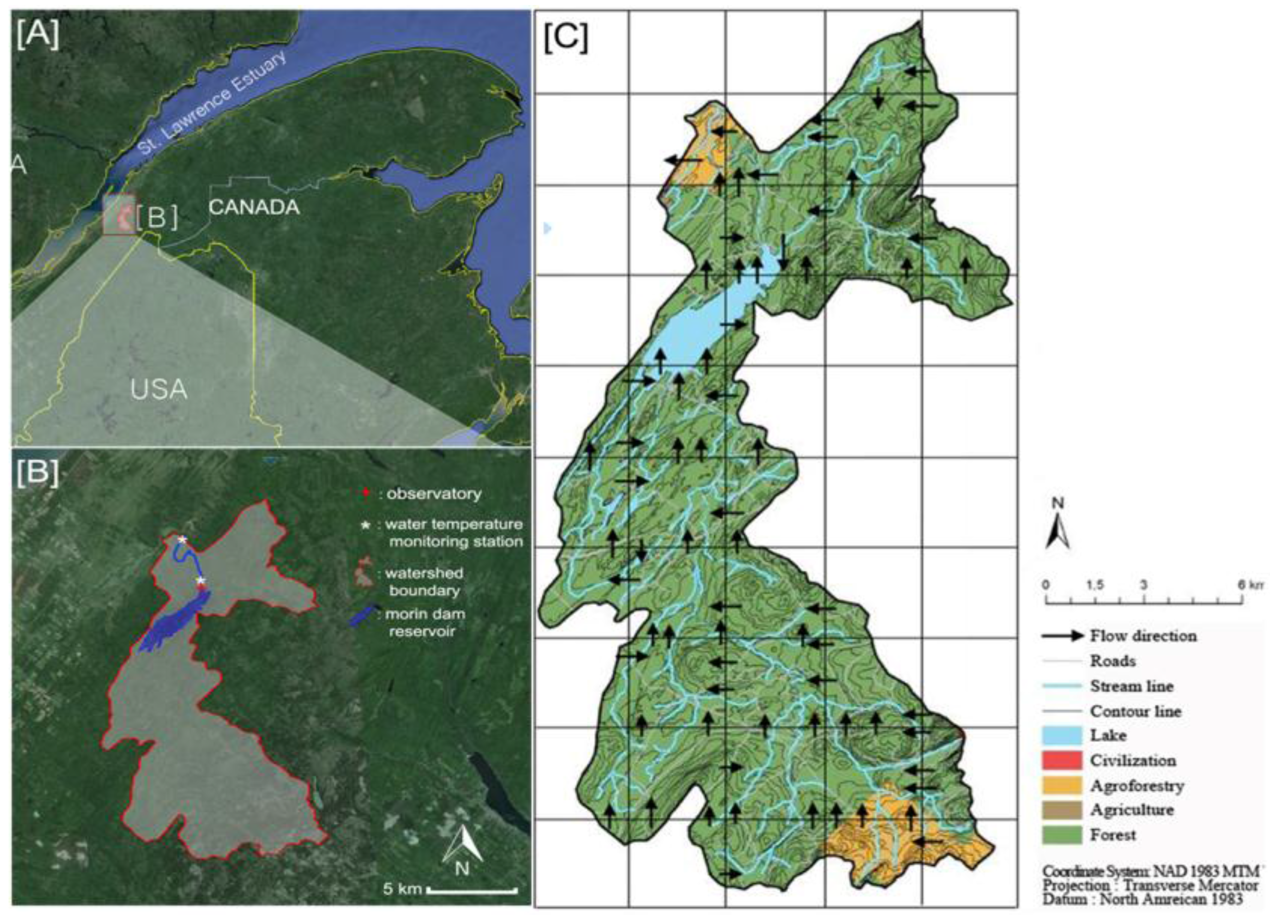
Figure 1. (A) Study area; (B) drainage basin showing location of reservoir; and (C) land use map showing hydrological units (whole squares) and arrows indicate water routing used for CEQUEAU.
Water 09 00346 g001
Figure 2. Schematic description of CEQUEAU model: (a) production function; and (b) routing function [39].
Water 09 00346 g002
Figure 3. Box plot of air temperature with 20 historical years and the four years with temperature measurements.
Water 09 00346 g003
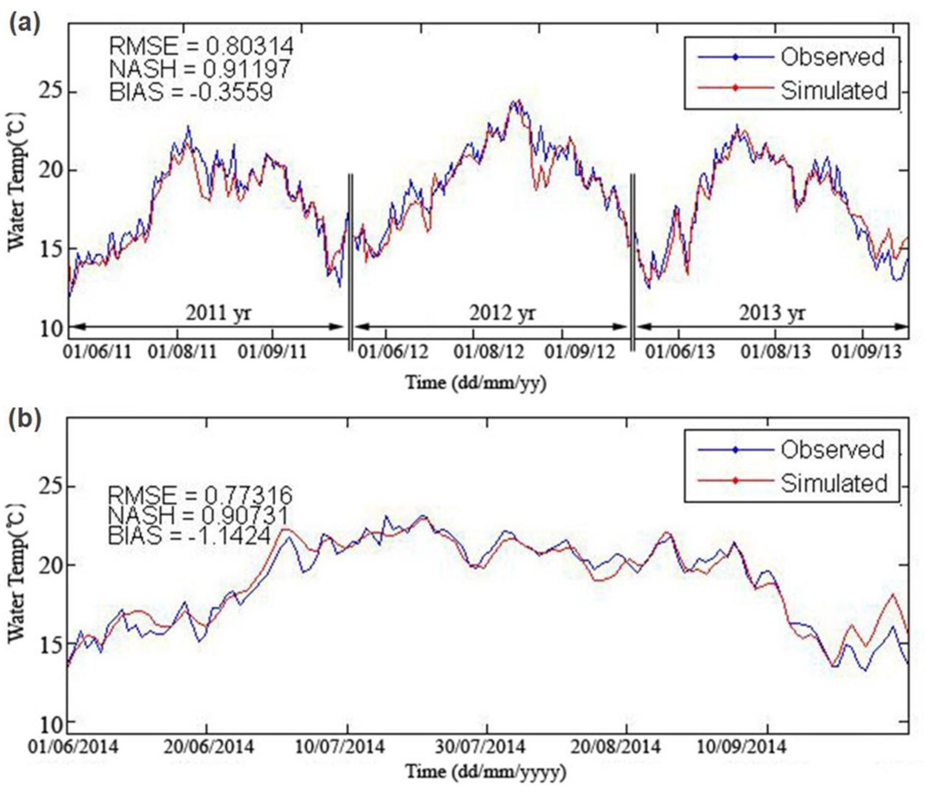
Figure 4. Observed and simulated flows with CEQUEAU hydrological model: (a) calibration (June 2011 to September 2013); and (b) validation periods (October 2013 to September 2014). Figure 5 shows observed and simulated daily water temperatures for the calibration and validation periods. Again, the model provided good results, with Nash coefficients above 0.9, RMSEs below 0.81. A systematic bias is observed during the calibration period and is exacerbated during the validation period, reaching −1.1 °C. This bias indicates that underestimation of the warmer temperatures in July and August by the model is likely.
Water 09 00346 g004
Figure 5. Observed and simulated water temperature during summer season with CEQUEAU hydrological model: (a) calibration (June to September 2011 to 2013); and (b) validation periods (June to September 2014).
Water 09 00346 g005
Figure 6. Two-variable Kolmogorov–Smirnov test (95% significance level) for RCP 2.6 for last 20 years (1994 to 2014): (*) indicated that the GCMs result identified as different distribution with observed.
Water 09 00346 g006
Figure 7. Boxplot of monthly median air temperature from 2020 to 2096 years for RCP 8.5 with 12 climate models; bold red line indicates monthly median air temperature for the observed period (2011 to 2014) and other results for RCP 2.6 (Figure S2) and RCP 4.5 (Figure S3) are in Supplementary Materials.
Water 09 00346 g007
Figure 8. Simulated result of runoff and water temperature based on MPI-ESM-LR climate model with RCP 2.6.
Water 09 00346 g008
Figure 9. Boxplot of daily water temperature (2016 to 2096 years) in summer season: (a) RCP 2.6 (9 climate models); (b) RCP 4.5 (12 climate models); and (c) RCP 8.5 (12 climate models) climate scenarios and bold red line indicate monthly median water temperature for observed period (2011 to 2014).
Water 09 00346 g009
Figure 10. Boxplot of number of the day over UILT of the brook trout for each RCP climate scenarios; RCP 2.6, RCP 4.5 and 8.5.
Water 09 00346 g010
Table 1. RCP (Representative Concentration Pathways) scenario description [54].
ScenariosDescriptionCO2 Concentration (ppm)Global Warming until 2100 (Mean and Likely Range)
RCP 2.6Peak in radiative forcing at ~3 W/m2 before 2100 year and then decline4901.0 (0.3–1.7) °C
RCP 4.5Stabilization without overshoot pathway to ~4.5 W/m2 at stabilization after 2100 year6501.8 (1.1–2.6) °C
RCP 6.0Stabilization without overshoot pathway to ~6 W/m2 at stabilization after 2100 year8502.2 (1.4–3.1) °C
RCP 8.5Rising radiative forcing pathway leading to 8.5 W/m2 by 2100 year13703.7 (2.6–4.8) °C
Table 2. GCMs used in this study and their modeling group [57].
#Modeling Center (or Group)GCMModel ExpansionSpatial Resolution
1Max Planck Institute for Meteorology (MPI-M)MPI-ESM-LR-r3Max Planck Institute Earth System Model, low resolution1.9° × 1.9°
210 km× 210 km
2Institute for Numerical MathematicsInmcm4-r1Institute of Numerical Mathematics Coupled Model, version 4.02° × 1.5°
220 km × 160 km
3Centre National de Recherches Météorologiques/Centre Européen de Recherche et Formation Avancée en Calcul ScientifiqueCNRM-CM5-r1Centre National de Recherches M_et_eorologiques Coupled Global Climate Model, version 5.11.4° × 1.4°
156 km × 156 km
4Commonwealth Scientific and Industrial Research Organization in collaboration with Queensland Climate Change Centre of ExcellenceCSIRO-Mk3.6.0-r1Commonwealth Scientific and Industrial Research Organisation Mark, version 3.6.01.8° × 1.8°
200 km × 200 km
5,6Met Office Hadley Centre (additional HadGEM2-ES realizations contributed by Instituto Nacional de Pesquisas Espaciais)HadGEM2-ES-r1Hadley Centre Global Environment Model, version 2–Earth System1.875° × 1.25°
HadGEM2-CC-r1208 km × 140 km
7Canadian Centre for Climate Modelling and AnalysisCanESM2-r1Second Generation Canadian Earth System Model2.8° × 2.8°
310 km × 310 km
8Meteorological Research InstituteMRI-CGCM3-r1Meteorological Research Institute Coupled Atmosphere–Ocean General Circulation Model, version 31.1° × 1.1°
110 km × 110 km
9National Center for Atmospheric ResearchCCSM4-r2Community Climate System Model, version 41.25° × 0.94°
140 km × 105 km
10Atmosphere and Ocean Research Institute (The University of Tokyo), National Institute for Environmental Studies, and Japan Agency for Marine-Earth Science and TechnologyMIROC5-r3Model for Interdisciplinary Research on Climate, version 51.4° × 1.4°
156 km × 156 km
11CSIRO (Commonwealth Scientific and Industrial Research Organisation, Australia), and BOM (Bureau of Meteorology, Australia)ACCESS1-0-r1Australian Community Climate and Earth-System Simulator, version 1.01.875° × 1.25°
208 km × 140 km
12NOAA Geophysical Fluid Dynamics LaboratoryGFDL-ESM2G-r1Geophysical Fluid Dynamics Laboratory Earth System Model with Generalized Ocean Layer Dynamics (GOLD) component (ESM2G)2.5° × 2.0°
280 km × 220 km
Table 3. Median daily water temperature with RCP climate scenarios.
Climate ScenariosMonthMedian Temperature (Degrees °C)
OBS (2011–2014)Sim. (2011–2014)Next Decade (2016–2025)Next 8 Decades (2016–2096)
RCP 2.6June15.8315.4216.07 (+0.2)16.04 (+0.2)
July21.1220.8221.39 (+0.3)21.50 (+0.4)
Aug.20.5420.2620.5520.60
Sep.16.1316.4515.42 (−0.7)15.96 (−0.2)
RCP 4.5June15.8315.4216.28 (+0.4)16.03 (+0.2)
July21.1220.8221.1720.91 (−0.2)
Aug.20.5420.2620.5720.55
Sep.16.1316.4515.52 (−0.6)15.45 (−0.7)
RCP 8.5June15.8315.4217.06 (+1.2)16.50 (+0.7)
July21.1220.8221.59 (+0.5)21.05
Aug.20.5420.2620.66 (+0.1)20.08 (−0.5)
Sep.16.1316.4515.40 (−0.7)14.97 (−1.1)
Table 4. Optimal and maximum temperature for salmonids.
SpeciesOptimal Temp. for Growth (°C)Maximum Temp. Upper Tolerances (°C) *Source
Rainbow trout (O. mykiss)15.0–19.024.0 *[66]
Brook trout(S. fontinalis)14.4–16.024.9[65]
* Based on the 95th percentile of maximum weekly mean temperatures where fish presence was observed [67].