
The Performance and Potentials of the CryoSat-2 SAR and SARIn Modes for Lake Level Estimation


Department of Geodesy, DTU Space, National Space Institute, 2800 Kgs. Lyngby, Denmark
*
Author to whom correspondence should be addressed.
Water 2017, 9(6), 374; https://doi.org/10.3390/w9060374
Submission received: 28 February 2017
/
Revised: 5 May 2017
/
Accepted: 19 May 2017
/
Published: 25 May 2017
(This article belongs to the Special Issue The Use of Remote Sensing in Hydrology)
Abstract
:Over the last few decades, satellite altimetry has proven to be valuable for monitoring lake levels. With the new generation of altimetry missions, CryoSat-2 and Sentinel-3, which operate in Synthetic Aperture Radar (SAR) and SAR Interferometric (SARIn) modes, the footprint size is reduced to approximately 300 m in the along-track direction. Here, the performance of these new modes is investigated in terms of uncertainty of the estimated water level from CryoSat-2 data and the agreement with in situ data. The data quality is compared to conventional low resolution mode (LRM) altimetry products from Envisat, and the performance as a function of the lake area is tested. Based on a sample of 145 lakes with areas ranging from a few to several thousand , the CryoSat-2 results show an overall superior performance. For lakes with an area below 100 , the uncertainty of the lake levels is only half of that of the Envisat results. Generally, the CryoSat-2 lake levels also show a better agreement with the in situ data. The lower uncertainty of the CryoSat-2 results entails a more detailed description of water level variations.
1. Introduction
Satellite altimetry has played an increasingly important role in lake level estimation over the past 20 years, where the number of gauges has been declining. The measuring technique provides almost global data sets, which makes it possible to study continental surface hydrology at all scales, independent of borders and national policies. The spatial and temporal coverage varies between missions. The TOPEX/Poseidon and the Jason 1–3 satellites were/are operating in a 10-day repeat cycle, while the European Remote Sensing (ERS) 1 and 2, Envisat, and Saral/Altika satellites were operating in a 35-day repeat cycle. Many of these conventional missions, with a footprint diameter of several kilometers, were originally intended for ocean applications. However, the use of satellite altimetry for inland water applications has evolved into a separate field of research. Some of the first results were obtained by [1], who estimated water level time series of lakes and reservoirs with the TOPEX/Poseidon satellite, and thereby demonstrating a successful use of satellite altimetry for hydrology applications. Since then, numerous studies have estimated not just the water levels of lakes from altimetry but also of rivers and wetlands. Ref. [2] combined lake levels obtained from different missions with bathymetry and imagery to derive changes in lake water storage. Ref. [3] studied annual water level oscillations of the remote Lake Namco on the Tibetan Plateau, and Ref. [4] used conventional altimetry together with high resolution imagery to estimate lake water storage of small lakes. Ref. [5] used Geosat altimetry data to estimate river levels at different positions of the Amazon river. Ref. [6] validated water levels obtained from the different retrackers available from Envisat over the Amazon basin with in situ data, and Ref. [7] demonstrated that reliable water level estimates can be obtained from Envisat over narrow branches of the Mekong River by accounting for the hooking effect. Ref. [8] derived water level heights for both rivers and wetlands from TOPEX/Poseidon, and Ref. [9] used 10 Hz data from TOPEX/Poseidon to study water level changes over Louisiana vegetated wetlands between 1992 and 2002. Ref. [10] studied seasonal water level variability of boreal wetlands in Western Siberia from Envisat. Over time, the data quality and the methodology to process the data have greatly improved. Currently, root mean square error (RMSE) estimates of just a few cm are obtained for selected lakes when comparing with in situ data [11].
CryoSat-2 and the recently launched Sentinel-3 represent a new generation of altimetry missions. These satellites apply Synthetic Aperture Radar (SAR) technology [12], which entails a reduction of the footprint in the along-track direction to approximately 300 m [13]. The smaller footprint size allows for monitoring much smaller lakes more accurately than previously. CryoSat-2 covers the Earth up to 88 degree latitude and has a repeat period of 369 days. The number of satellite crossings over a given lake therefore depends on the lake extent in the east–west direction and the latitude [14]. Hence, smaller lakes are not visited sufficiently to capture the seasonal signal. On the other hand, significantly more lakes are visited. Recently, some studies regarding lake level estimation including new processing strategies of CryoSat-2 data have been carried out. Ref. [15] presented a new waveform retracker based on cross-correlation of a modeled CryoSat-2 waveform with the observed waveforms. Ref. [16] demonstrated that the SAR mode provides an increased precision for small lakes compared to conventional altimetry. Ref. [11] presented a novel SAR mode retracker, which utilizes information from several waveforms simultaneously, and [17] demonstrated that waveform classification might be a powerful tool to handle erroneous data. Ref. [14,18] used CryoSat-2 data to investigate the trend and seasonal signal of lakes on the Tibetan Plateau.
Here, we intend to quantify the quality of CryoSat-2 data in the SAR and SARIn modes for lake level estimation and prove its better performance over smaller lakes compared to conventional altimetry from Envisat. This has previously only been done in studies where a few lakes were investigated [16,17].
To quantify the quality of the lake levels derived from CryoSat-2, we perform a thorough investigation of the performance of CryoSat-2 compared to conventional altimetry as observed by Envisat. The study is based on a set of 145 lakes which are covered by both CryoSat-2 (SAR or SARIn mode) and Envisat (LRM). The lakes are located in Canada, Finland, and Denmark and have areas ranging from a few to several thousand . A way to evaluate the data is to consider the standard deviation of the predicted water level for each crossing over a given lake. For each lake, the standard deviations are summarized by the median, which hereafter is referred to as the median of standard deviation (MSD). The MSD gives a measure of how accurately the water level is estimated, which subsequently determines how small water level variations that can be observed. We estimate the MSD for each lake and test its dependence on lake area, in order to evaluate the improvement available with the new altimetry modes. In situ data is available for selected Canadian lakes, which enables the evaluation of the ability to capture annual and interannual signals. Finally, the mean water level of Danish lakes is evaluated against accurate laser scanner data.
2. Deriving Water Levels from Satellite Altimetry
In satellite altimetry [19], the distance to the surface, the range R, is measured. This is done by emission of an electromagnetic transmitted pulse traveling with the speed of light. The reflected signal is subsequently received by the antenna on-board the satellite. The range is derived from the two-way travel time of the pulse. Assuming the altitude h of the satellite is known with respect to a reference ellipsoid, the surface elevation H relative to this ellipsoid is given by the following simple relation (see Figure 1):
The range provided by the satellite is often referenced to the center of the range window and is therefore only an approximate estimate (see Figure 1 and Figure 2). The range window is the area in the direction of the pulse where the satellite can pick up the reflected signal. For CryoSat-2, the range window is 60 and 240 m for for the SAR and SARIn modes, respectively. To estimate the exact range, on-ground processing, referred to as retracking, must be performed. Retracking is the procedure of identifying the surface on the leading edge of the waveform (see Figure 2). The waveform is the received power as a function of the power bins in the range window. In empirical retracking, the surface or retracking point is typically defined as the decimal bin along the leading edge, which is associated with a certain power threshold. The distance between the center bin and the retracking point in the waveform defines the retracking correction (see Figure 2).
The range must also be corrected for any path delay that occurs when the signal travels through the atmosphere and for geophysical signals that influence the elevation of the water surface. Hence, the range is corrected for the ionosphere, wet and dry troposphere, solid Earth tide, ocean loading tide, and geocentric polar tide, which are combined in the correction term . The water level above a reference geoid N is derived from the following expression:
3. Study Area
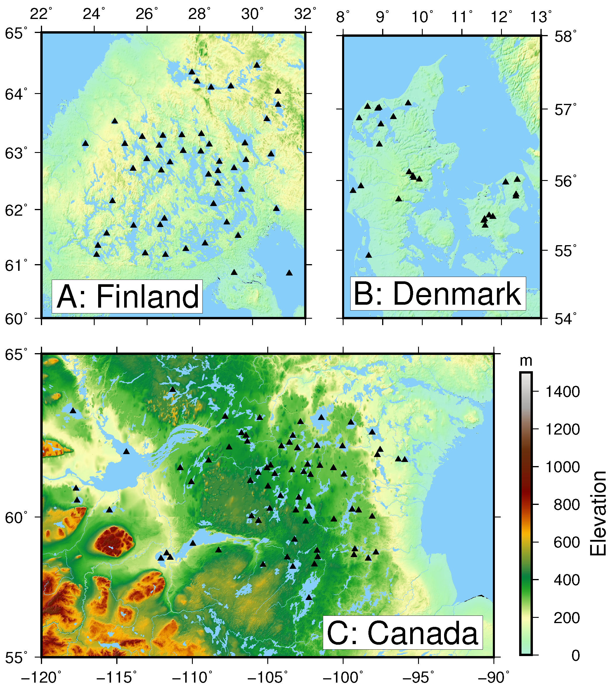
To evaluate the performance of both the SAR and SARIn modes, several relevant regions in Canada, Finland and Denmark are selected. These regions have a large concentration of lakes. There are 25 Danish lakes included in the study, which all are smaller than 40 . These lakes are situated in a relatively flat terrain. In this area, CryoSat-2 is operating in the SAR mode. There is a total of 120 Finish and Canadian lakes, which are covered by CryoSat-2 in SARIn mode, and these lakes range in area from 51 to 27,816 . A large fraction of the lakes has complex coastlines and several small islands. Figure 3 displays the study areas: A, Finland, B, Denmark, and C, Canada. The location of the lakes is marked with triangles.
4. Data
We use the CryoSat-2 European Space Agency (ESA) L1b baseline C and the Envisat Radar Altimetry (RA) Geophysical Data Record (GDR) data products, which are thoroughly described in the following subsections. These products also include the geophysical corrections described above. The applied geoid model is the Earth Gravitational Model 2008 (EGM2008) [20]. To extract measurements from water returns, lake masks from the Global Lakes and Wetlands Database [21] and the Danish Geodata Agency [22] are applied.
4.1. Envisat
Envisat operated from 2002 to 2012 in a 35-day repeat cycle, with a distance between tracks of approximately 85 km at the Equator. The Radar Altimeter 2 (RA-2) onboard Envisat was a dual-frequency altimeter operating at Ku- and S-band, with the Ku-band channel being the primary altimetry radar and the additional S-band channel being used to correct for ionospheric effect. The Ku radar operated as a pulse-limited altimeter which emitted pulses at 1800 Hz, but with a subsequently averaging of 100 return pulses onboard the satellite, resulting in an 18 Hz product being transmitted to the ground stations. The pulse-limited altimeter gives circular footprints which are slightly elongated in the along-track direction due to the averaging of the return pulses. The size of the RA2 footprint was 10 km to 15 km depending on the height distribution within the illuminated surface area. In this study, we use the range measurements based on the Ice1 retracker [23], which is based on the Offset Center of Gravity (OCOG) retracker.
4.2. CryoSat-2
The CryoSat-2 satellite was launched in 2010. The SAR Interferometer Radar Altimeter (SIRAL) onboard CryoSat-2 is a single frequency Ku band altimeter capable of operating in three different modes: Low Resolution Mode (LRM), SAR mode, and SARIn mode. In LRM, the SIRAL operates like a conventional altimeter with properties comparable to RA2; however, to allow seamless switch between the different modes, it emits pulses at 1970 Hz. In SAR mode, the pulse repetition frequency (PRF) is increased to 17.8 kHz and pulses are emitted in bursts of 64 pulses. The high PRF ensures that the return pulses are correlated, and it is therefore possible to apply Doppler processing of the 64 pulses. In the Doppler processing, it is possible to divide the area illuminated by all 64 pulses into 64 areas in the along-track direction. The result is a footprint that is pulse limited in the across-track direction and Doppler limited in the along-track direction. The Doppler beams from different bursts that illuminate a selected area on the ground are then averaged to form the waveform. Since the along-track footprint is Doppler-limited, it is not dependent on the height distribution within the illuminated area. The SARIn mode is similar to the SAR mode but includes an additional receiving antenna that allows determination of the position of the reflecting surface in the across-track direction.
The CryoSat-2 data contains waveforms with 256 and 1024 bins for SAR and SARIn, respectively. The waveforms are retracked by an empirical sub-waveform retracker; the Narrow Primary Peak Threshold (NPPT) [24], which is part of the Lars Advanced Retracking System (LARS) [25]. In SARIn, it is possible to correct the range for off-nadir returns, and, in this study, this correction is performed according to [26].
4.3. In-Situ Data
Height measurements from a national survey were extracted for a subset of the Danish lakes. The survey was conducted in 2014 and 2015 with the aim to improve the Danish elevation model. The data set contains laser scanner data with a point density of four to five measurements per square meter. The heights are referenced to DVR90, but has been converted to heights above the WGS84 reference ellipsoid with the software “KMSTRANS” [27]. The error of the data is less than 5 cm in the vertical direction. The data is available from [22].
In situ data of the water level is freely available for several lakes in Canada from the Government of Canada [28]. Lakes in the study area, which are measured with both CryoSat-2 and Envisat and where in situ data is available, are Great Slave, Athabasca, Wollaston, Claire, Nonacho, and Reindeer. The water levels are referenced to different datums, e.g., the Geodetic Survey of Canada Datum.
5. Methods and Data Processing
Waveforms related to returns from inland water might be multi-peaked due to land contamination in the signal or from the presence of strong off-nadir signals. Such complex waveforms might result in noisy and potentially erroneous water levels, and it is essential to handle these in a robust manner.
To construct lake level time series, we follow the approach described in [16], in which a state-space model is used to reconstruct the time series. The model consists of a process part and an observation part. The process part intends to describe how the true water levels vary over time. It is implemented as a random walk, which implies that water levels measured within a short time span will tend to be more alike. The observation part describes how the measurements relate to the true water level. The measurement distribution is described by a mixture between a Gaussian and a Cauchy distribution. Compared to a pure Gaussian distribution, this describes the situation where a fraction of the measurements is wrong or extremely noisy. The heavier tails of the Cauchy distribution will have the effect of reducing the influence of such erroneous observations. The described state-space model represents a robust model in the sense that the estimated water levels are not substantially biased by erroneous observations. The process enables the model to exploit the temporal correlation in the true water levels. A detailed description of the model is found in [16].
The state-space model has been implemented in a software package “tsHydro” written in the open source language “R”. The package is built via the R-Package Template Model Builder (TMB) [29], which is a tool to construct complex state-space models using Automatic Differentiation and the Laplace approximation to obtain accurate and stable optimization [30]. The package offers the user the possibility to easily estimate robust water levels. To construct time series, the user must provide an input file that contains the following columns, the time in decimal years, the track number and the raw water levels. The program returns the predicted water level at each time step together with its standard deviation. The package is freely available from Github [31].
Before applying the “tsHydro” package, a rough outlier criterion is applied. For each lake, the median of all water levels is estimated. Subsequently, water levels above and below the median ±5 m are removed. A limit of 5 m is not recommended in general, since lake levels may vary several meters over time. However, for the lakes in this study, a limit of 5 m was found appropriate.
The MSD is used as a summary measure of the uncertainty for each data type (), CryoSat-2 or Envisat, at each lake. We wish to quantify and test if the different data types result in different levels of uncertainty. It is also expected that the lake area has an influences on the uncertainty, which must be taken into account. The lakes are divided into three groups () defined by their area: small <100 , medium 100–1000 , or large >1000 . Each uncertainty measurement, MSD, is described by the following standard two-way analysis of variance (ANOVA) model:
Here, , where N is the number of observations. is a common intercept. The model parameters describe the main effect of the data types. The model parameters describe the main effects of the lake area groups. The model parameters describe the interaction effect between the lake area group and data types. The interaction term describes how the effect of data types differs in the various lake area groups. If the hypothesis is rejected (by a standard F-test), then the effect of data types is not the same in all lake area groups. The noise term for the logarithm of the MSDs is assumed to follow a normal distribution .
6. Results
In this study, we have predicted CryoSat-2 and Envisat water levels for 145 lakes to evaluate the performance of the SAR and SARIn modes compared to conventional altimetry.
6.1. Evaluation of MSD, Uncertainty
The median of the standard deviations of the predicted water levels, MSD, which is a measure of the uncertainty, was evaluated for all lakes. Figure 4A displays the estimated MSD of CryoSat-2 and Envisat as a function of the lake area. The MSDs of the CryoSat-2 and Envisat results lie in the range of 1–8 cm and 1–28 cm, respectively. The MSD of the CryoSat-2 results is generally lower, where the most pronounced difference is seen for lakes with a small area. For large lakes, the MSD is similar for the two data sets. Figure 4B displays the MSD ratio, showing Envisat over CryoSat-2, as a function of the lake area. Values above and below 1 indicate lakes where the CryoSat-2 or Envisat results have the lowest MSD, respectively. For most lakes, this ratio demonstrates that the MSD of CryoSat-2 is less than half as the MSD of Envisat.
6.2. The Significance of Lake Area with Respect to MSD
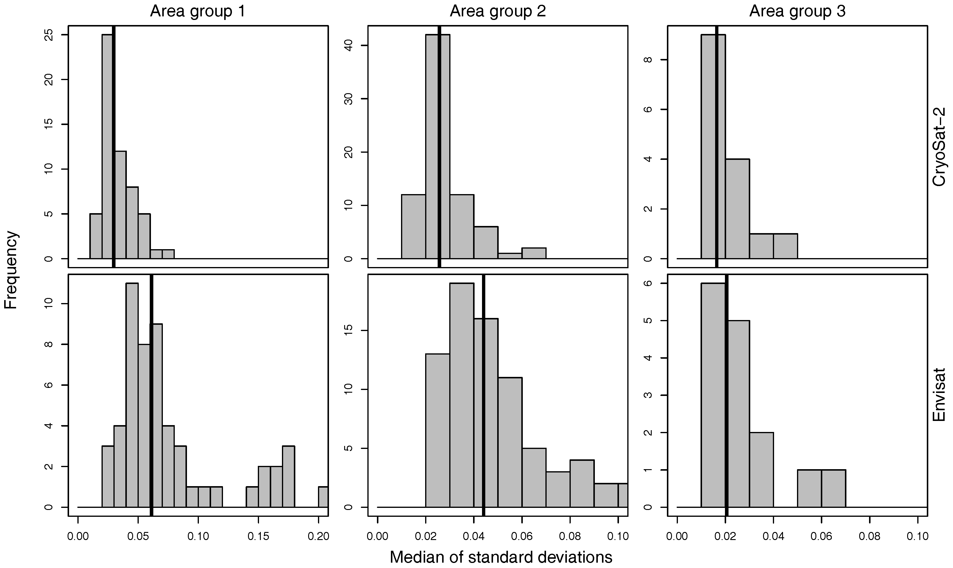
The model for the logarithm of the median of standard deviations (3) was validated by visual inspection of the residuals. The hypothesis that the difference between the two data types is the same for all three area groups was rejected by a standard F-test (p-value 0.006716). The difference between the two data types is different for the three area groups. For the smallest area group, the MSD was 2.2 times higher for Envisat than for CryoSat-2 with a 95% confidence interval of [1.9–2.7]. For the medium area group, the MSD was 1.7 times higher for Envisat with a confidence interval of [1.5–2.0]. Finally, for the largest area group, the MSD was 1.3 times higher for the Envisat, but the difference was not significant, as the confidence interval [0.9–1.8] included 1. A detailed description of the MSD distributions for the three area groups are shown in Figure 5.
6.3. Comparison with In Situ Data
6.3.1. Canadian Lakes
The second measure of performance of CryoSat-2 and Envisat to measure water level variations is the agreement with the true water level. The true water level is represented by in situ measurements of the water level. In situ measurements are available for six Canadian lakes: Great Slave Lake, Lake Athabasca, Reindeer Lake, Lake Wollaston, Lake Claire, and Lake Nonacho. Since the satellite and the in situ data are referenced with respect to different datums, a bias in the water levels is estimated and subtracted from the satellite data. Figure 6 shows the estimated time series of the water level together with the in situ data for the six lakes. The circles represent the water level of the retracked data, while the crosses represent the model based predictions. In general, the predicted satellite-based time series follow the in situ data quite well. For the lakes Wollaston, Nonacho, and Reindeer, the CryoSat-2 based time series give a better representation of the water level variations than the Envisat based solution. This is quantified by RMSE estimates, which are listed in Table 1. For Great Slave Lake, both satellite based models reveal erroneous water level estimates, although the overall variation is well represented. These estimates result in an artificially increased RMSE value.
6.3.2. Danish Lakes
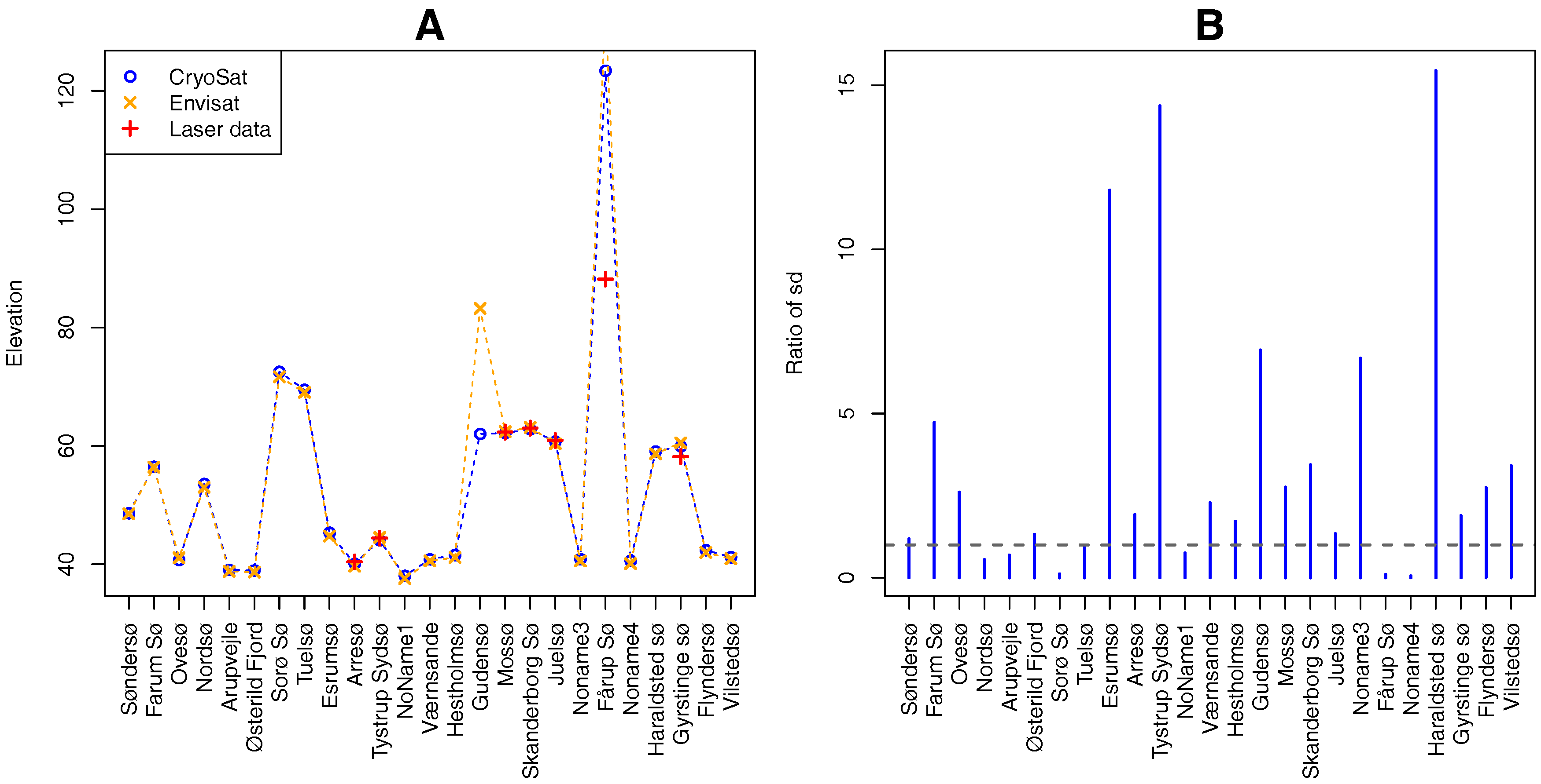
Here, we compare the laser based heights with the mean water levels obtained from CryoSat-2 and Envisat. To account for the range bias between the two missions, the Envisat heights have been corrected with a bias of −0.69 cm [32] to be comparable with the CryoSat-2 heights. The mean water level for each lake is constructed as a weighted average of the predicted water levels for each crossing. Figure 7A displays the height with respect to the WGS84 reference ellipsoid for the laser, CryoSat-2, and Envisat data. The height estimates and their corresponding standard deviations are collected in Table 2. The agreement between the satellite based estimates and the laser scanner data is generally good, except for the lake Fårup Sø. For the lake Gudensø, there is a discrepancy between the CryoSat-2 and the Envisat estimates. Figure 7B displays the ratio of standard deviations. As indicated by Figure 7B, the CryoSat-2 based solutions generally have a smaller standard deviation.
7. Discussion
The water level for each crossing, based on CryoSat-2 and Envisat data, was estimated for 145 lakes with areas between 1 and 27,816 . The MSDs of the CryoSat-2 and Envisat results were compared, and the predicted water levels were compared with in situ data. In the following, the applied methodology and the results are discussed in detail.
As expected, the new modes, SAR and SARIn, generally lead to an improved estimate of the water level compared to conventional altimetry. The analysis performed here has quantified that the effect is most pronounced for smaller lakes. For larger lakes, the lower uncertainty is insignificant due to the larger number of measurements. Here, it should be mentioned that, despite the high quality of the CryoSat-2 data as demonstrated in Figure 5, the uncertainty is also affected by the lake setting because topography and off-nadir signals may considerably increase the noise in the data. An example of this is seen for the Danish lake Fårup Sø in Figure 7. This lake has an area of just 0.96 . The terrain surrounding this lake is relatively steep and in the vicinity smaller lakes located at a higher elevation are present. This configuration of terrain and surrounding lakes causes the water levels to be incorrectly estimated in the retracking process. However, by inspecting the retracked water levels, CryoSat-2 is actually able to capture the “correct” water level at some crossings (see Appendix A).
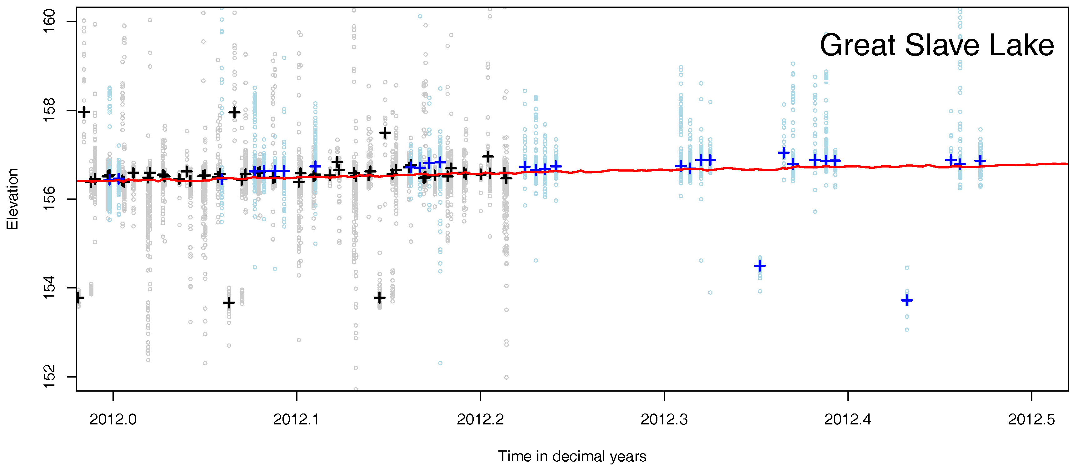
Estimating the water level for inland water bodies is challenging, since the raw retracked measurement can be noisy and erroneous (Figure 6), which easily influences the estimate. However, a robust method here that is able to account for erroneous observations in an objective manner was used. The estimates are, therefore, less sensitive to outlying observations (see Figure 6). For Great Slave Lake, a large fraction of erroneous water level estimates is present for both data sets. The applied method is clearly unable to detect the “correct” water level in this case. However, a closer inspection of the data reveals groups of erroneous data at these times (see Figure 8). In fact, at most of these times, no data at the “correct” level is present. The large fraction of erroneous data causes the state-space model to give the data a too high weight compared to the underlying process. This results in a wrong estimate of the water level. Situations like these are a weakness of the applied model. It is possible that a future extension of the model to account for the correlation between observations on the same track could reduce the weight of such sets of incorrect observations, which could give a more correct reconstruction.
Here, we have chosen to use the MSD as a measure of quality, since it represents the uncertainty of the estimated water level for a given crossing. The individual observations are often very noisy and mixed with outliers, hence the MSD of the estimated lake level is a more accurate measure with respect to the usefulness of the data. It is a measure of how detailed the water level can be described over time. The temporal variations of the lake level can be tracked in greater details when the MSD is at a low level.
For a subset of the Danish lakes, the satellite-based mean water levels above WGS84 were compared to laser scanner data collected between 2014 and 2015 (Figure 7). Both data sets showed a good agreement. The minor height difference might partly be explained by the retracking bias which can be of several cm or small variations in the inter-mission bias. Furthermore, the laser data were collected after the time period of the Envisat data. However, the water level variation of Danish lakes is small. Based on Google Earth, the lake Gudensø has an elevation similar to the lakes Mossø, Juelsø, and Skanderborg Sø. This indicates that the CryoSat-2 based height is closer to the “correct” height.
8. Conclusions
Based on the results found in this study, it can be concluded that the CryoSat-2 derived lake levels have a significant lower MSD compared to Envisat for lakes with an area smaller than 1000 . Furthermore, the CryoSat-2 results show an overall better agreement with in situ data for the six Canadian lakes. The RMSE values are in the range of 5–68 cm and 17–54 cm for CryoSat-2 and Envisat, respectively. Both CryoSat-2 and Envisat based mean water levels agreed well with the laser scanner data. These results reveal a promising potential of Sentinel-3, which is operating in the SAR mode globally with a repeat period of 27 days. Hence, assuming that the data quality of Sentinel-3 resembles that of CryoSat-2, water level variations below 10 cm can potentially be captured for relatively small lakes.
Acknowledgments
We acknowledge the FP7 project Land and Ocean take up from Sentinel-3 (LOTUS) under Grant No. 313238 that has partly funded this work. Anders Nielsen is acknowledged for statistical guidance. Louise Sandberg Sørensen and Stine Kildegaard Rose are acknowledged for language editing. Finally, we acknowledge the anonymous reviewers for improving the manuscript.
Author Contributions
Karina Nielsen processed CryoSat-2 data, conducted the analysis, and wrote the majority of the manuscript. Lars Stenseng processed CryoSat-2 and contributed to manuscript writing. Ole B. Andersen and Per Knudsen contributed with discussions and manuscript writing.
Conflicts of Interest
The authors declare no conflict of interest.
Appendix A
Table A1 shows all the observed water levels of Fårup Sø from CryoSat-2 and Envisat.

Table A1.
Water levels of Fårup Sø.
| Time CryoSat-2 | Height CryoSat-2 | Time Envisat | Height Envisat |
|---|---|---|---|
| 2011.259 | 126.881 | 2003.367 | 133.756 |
| 2011.259 | 161.100 | 2003.750 | 110.016 |
| 2011.616 | 112.106 | 2004.612 | 141.591 |
| 2011.616 | 105.081 | 2004.994 | 132.531 |
| 2013.631 | 147.994 | 2005.186 | 134.269 |
| 2013.631 | 147.963 | 2005.953 | 139.167 |
| 2014.640 | 112.315 | 2007.008 | 138.599 |
| 2014.640 | 88.106 | 2008.636 | 110.615 |
| 2015.292 | 88.038 | 2009.690 | 110.621 |
| 2015.292 | 88.019 | 2010.265 | 136.480 |
| 2015.648 | 125.739 | 2010.745 | 110.055 |
| 2015.648 | 125.606 | ||
| 2016.656 | 148.264 | ||
| 2016.656 | 148.020 |
References
- Birkett, C.M.B. The contribution of TOPEX/POSEIDON to the global monitoring of climatically sensitive lakes. J. Geophys. Res. 1995, 100204, 25179–25204. [Google Scholar] [CrossRef]
- Crétaux, J.F.; Birkett, C. Lake studies from satellite radar altimetry. C. R. Geosci. 2006, 338, 1098–1112. [Google Scholar] [CrossRef]
- Kropáček, J.; Braun, A.; Kang, S.; Feng, C.; Ye, Q.; Hochschild, V. Analysis of lake level changes in Nam Co in central Tibet utilizing synergistic satellite altimetry and optical imagery. Int. J. Appl. Earth Obs. Geoinf. 2012, 17, 3–11. [Google Scholar] [CrossRef]
- Baup, F.; Frappart, F.; Maubant, J. Combining high-resolution satellite images and altimetry to estimate the volume of small lakes. Hydrol. Earth Syst. Sci. 2014, 18, 2007–2020. [Google Scholar] [CrossRef]
- Koblinsky, C.J.; Clarke, R.T.; Brenner, A.C.; Frey, H. Measurement of river level variations with satellite altimetry. Water Resour. Res. 1993, 29, 1839–1848. [Google Scholar] [CrossRef]
- Frappart, F.; Calmant, S.; Cauhopé, M.; Seyler, F.; Cazenave, A. Preliminary results of ENVISAT RA-2-derived water levels validation over the Amazon basin. Remote Sens. Environ. 2006, 100, 252–264. [Google Scholar] [CrossRef]
- Boergens, E.; Dettmering, D.; Schwatke, C.; Seitz, F. Treating the Hooking Effect in Satellite Altimetry Data: A Case Study along the Mekong River and Its Tributaries. Remote Sens. 2016, 8, 91. [Google Scholar] [CrossRef]
- Birkett, C.M. Contribution of the TOPEX NASA Radar Altimeter to the global monitoring of large rivers and wetlands. Water Resour. Res. 1998, 34, 1223–1239. [Google Scholar] [CrossRef]
- Lee, H.; Shum, C.K.; Yi, Y.; Ibaraki, M.; Kim, J.W.; Braun, A.; Kuo, C.Y.; Lu, Z. Louisiana wetland water level monitoring using retracked TOPEX/POSEIDON altimetry. Mar. Geod. 2009, 32, 284–302. [Google Scholar] [CrossRef]
- Zakharova, E.A.; Kouraev, A.V.; Rémy, F.; Zemtsov, V.A.; Kirpotin, S.N. Seasonal variability of the Western Siberia wetlands from satellite radar altimetry. J. Hydrol. 2014, 512, 366–378. [Google Scholar] [CrossRef]
- Villadsen, H.; Deng, X.; Andersen, O.B.; Stenseng, L.; Nielsen, K.; Knudsen, P. Improved inland water levels from SAR altimetry using novel empirical and physical retrackers. J. Hydrol. 2016, 537, 234–247. [Google Scholar] [CrossRef]
- Raney, R.K. The delay/Doppler radar altimeter. IEEE Trans. Geosci. Remote Sens. 1998, 36, 1578–1588. [Google Scholar] [CrossRef]
- Wingham, D.J.; Francis, C.R.; Baker, S.; Bouzinac, C.; Brockley, D.; Cullen, R.; de Chateau-Thierry, P.; Laxon, S.W.; Mallow, U.; Mavrocordatos, C.; et al. CryoSat: A mission to determine the fluctuations in Earth’s land and marine ice fields. Adv. Space Res. 2006, 37, 841–871. [Google Scholar] [CrossRef]
- Kleinherenbrink, M.; Lindenbergh, R.; Ditmar, P. Monitoring of lake level changes on the Tibetan Plateau and Tian Shan by retracking Cryosat SARIn waveforms. J. Hydrol. 2015, 521, 119–131. [Google Scholar] [CrossRef]
- Kleinherenbrink, M.; Ditmar, P.; Lindenbergh, R. Retracking Cryosat data in the SARIn mode and robust lake level extraction. Remote Sens. Environ. 2014, 152, 38–50. [Google Scholar] [CrossRef]
- Nielsen, K.; Stenseng, L.; Andersen, O.B.; Villadsen, H.; Knudsen, P. Validation of CryoSat-2 SAR mode based lake levels. Remote Sens. Environ. 2015, 171, 162–170. [Google Scholar] [CrossRef]
- Göttl, F.; Dettmering, D.; Müller, F.; Schwatke, C. Lake Level Estimation Based on CryoSat-2 SAR Altimetry and Multi-Looked Waveform Classification. Remote Sens. 2016, 8, 885. [Google Scholar] [CrossRef]
- Jiang, L.; Nielsen, K.; Andersen, O.B.; Bauer-Gottwein, P. Monitoring recent lake level variations on the Tibetan Plateau using CryoSat-2 SARIn mode data. J. Hydrol. 2017, 544, 109–124. [Google Scholar] [CrossRef]
- Fu, L.L.; Cazenave, A. Satellite Altimetry and Earth Sciences: A Handbook of Techniques and Applications; Academic: San Diego, CA, USA, 2001; p. 463. [Google Scholar]
- Pavlis, N.K.; Holmes, S.A.; Kenyon, S.C.; Factor, J.K. The development and evaluation of the Earth Gravitational Model 2008 (EGM2008). J. Geophys. Res. Solid Earth 2012, 117. [Google Scholar] [CrossRef]
- Lehner, B.; Döll, P. Development and validation of a global database of lakes, reservoirs and wetlands. J. Hydrol. 2004, 296, 1–22. [Google Scholar] [CrossRef]
- Kortforsyningen. Available online: http://kortforsyningen.dk/ (accessed on 23 May 2017).
- Bamber, J.L. Ice sheet altimeter processing scheme. Int. J. Remote Sens. 1994, 15, 925–938. [Google Scholar] [CrossRef]
- Villadsen, H.; Andersen, O.B.; Stenseng, L.; Nielsen, K.; Knudsen, P. CryoSat-2 altimetry for river level monitoring—Evaluation in the Ganges–Brahmaputra River basin. Remote Sens. Environ. 2015, 168, 80–89. [Google Scholar] [CrossRef]
- Stenseng, L.; Andersen, O.B. Preliminary gravity recovery from CryoSat-2 data in the Baffin Bay. Adv. Space Res. 2012, 50, 1158–1163. [Google Scholar] [CrossRef]
- Armitage, T.W.K.; Davidson, M.W.J. Using the interferometric capabilities of the ESA Cryosat-2 mission to improve the accuracy of sea ice freeboard retrievals. IEEE Trans. Geosci. Remote Sens. 2014, 52, 529–536. [Google Scholar] [CrossRef]
- Kmstrans. Available online: https://bitbucket.org/KMS/kmstrans (accessed on 23 May 2017).
- Government of Canada. Water Level and Flow. Available online: https://wateroffice.ec.gc.ca/ (accessed on 23 May 2017).
- Kristensen, K.; Nielsen, A.; Berg, C.W.; Skaug, H.; Bell, B.M. TMB: Automatic differentiation and laplace approximation Authors. J. Stat. Softw. 2016, 70, 1–21. [Google Scholar] [CrossRef]
- Skaug, H.J.; Fournier, D.A. Automatic approximation of the marginal likelihood in non-Gaussian hierarchical models. Comput. Stat. Data Anal. 2006, 51, 699–709. [Google Scholar] [CrossRef]
- Github. Available online: https://github.com/cavios/tshydro (accessed 23 May 2017).
- Bosch, W.; Dettmering, D.; Schwatke, C. Multi-Mission Cross-Calibration of Satellite Altimeters: Constructing a Long-Term Data Record for Global and Regional Sea Level Change Studies. Remote Sens. 2014, 6, 2255–2281. [Google Scholar] [CrossRef]
Figure 1.
The principle of satellite altimetry.
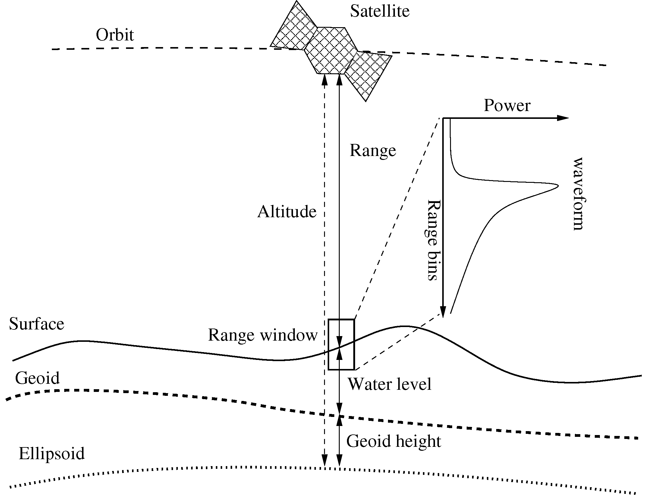
Figure 2.
Explanation of the retracking correction.
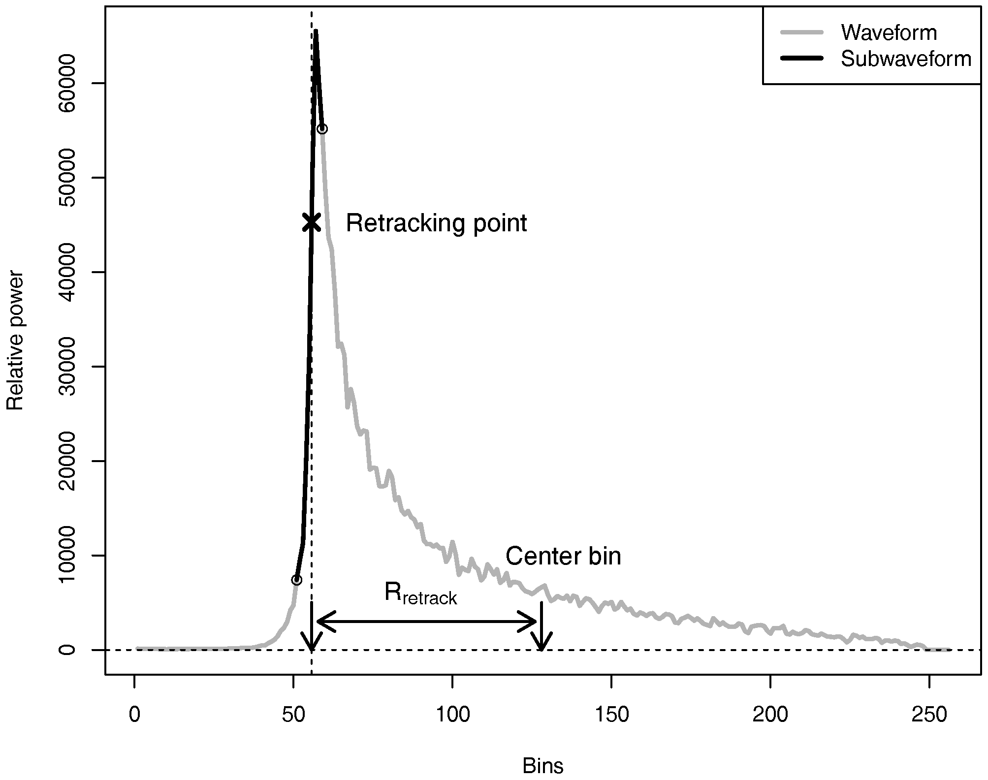
Figure 3.
An overview of the lakes included in the study.

Figure 4.
(A) the MSD of CryoSat-2 (blue) and Envisat (orange) as a function of Area; (B) the MSD ratio as a function of area. Values above and below 1 indicate ratios, where CryoSat-2 or Envisat have the lowest MSD, respectively.
Figure 4.
(A) the MSD of CryoSat-2 (blue) and Envisat (orange) as a function of Area; (B) the MSD ratio as a function of area. Values above and below 1 indicate ratios, where CryoSat-2 or Envisat have the lowest MSD, respectively.
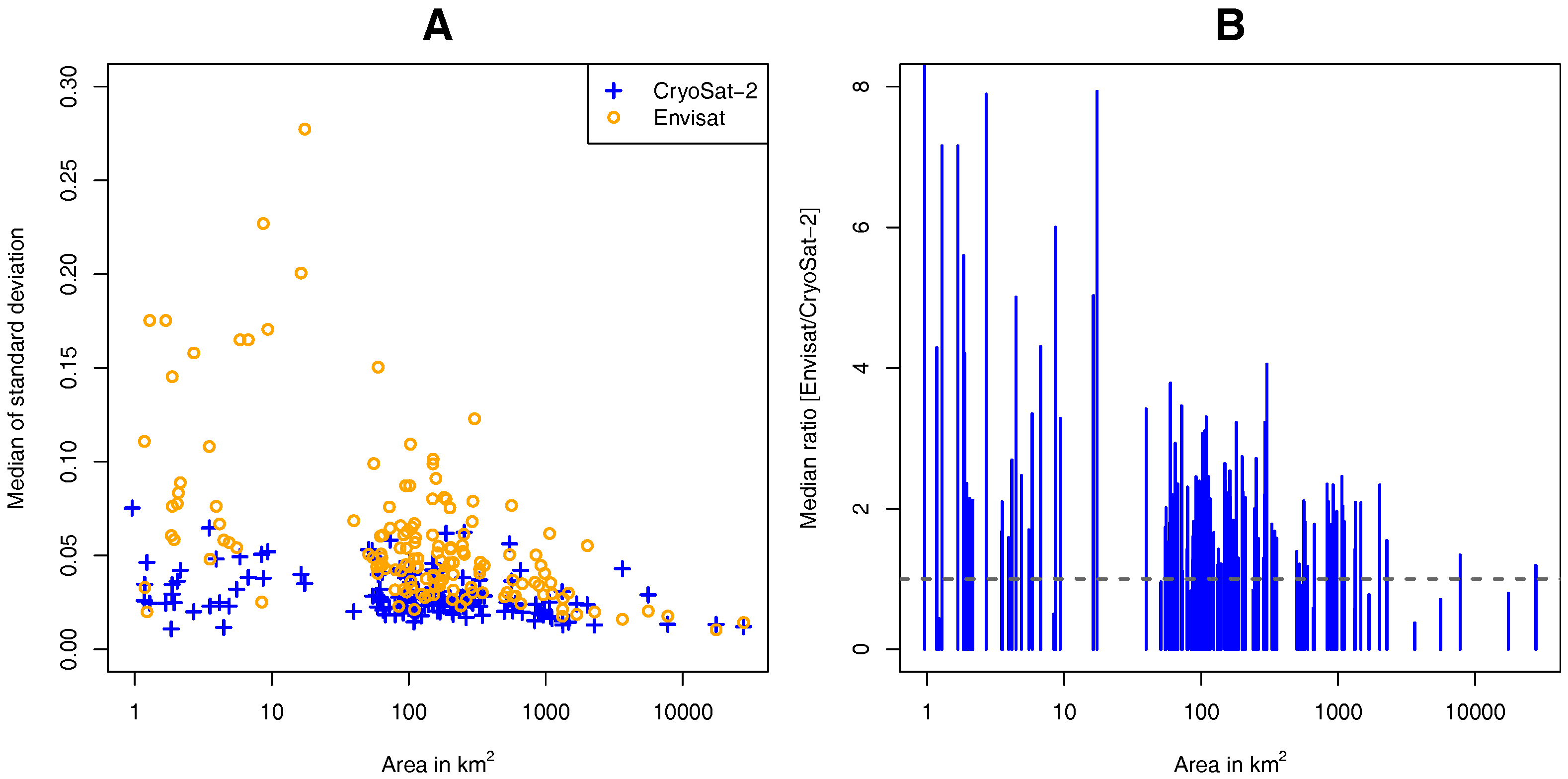
Figure 5.
Histograms of MSD for CryoSat-2 and Envisat in the three area groups; group 1 (<100 ), group 2, (100–1000 ), and group 3 (>1000 ). The vertical black line indicates the median of the MSDs.
Figure 5.
Histograms of MSD for CryoSat-2 and Envisat in the three area groups; group 1 (<100 ), group 2, (100–1000 ), and group 3 (>1000 ). The vertical black line indicates the median of the MSDs.

Figure 6.
Water level time series for the six Canadian lakes: Great Slave, Athabasca, Wollaston, Claire, Nonacho, and Reindeer. The gray (Envisat) and blue (CryoSat-2) circles represent the raw retracked water levels. The black (Envisat) and blue (CryoSat-2) crosses represent the predicted water level, and the red line is the in situ water levels.
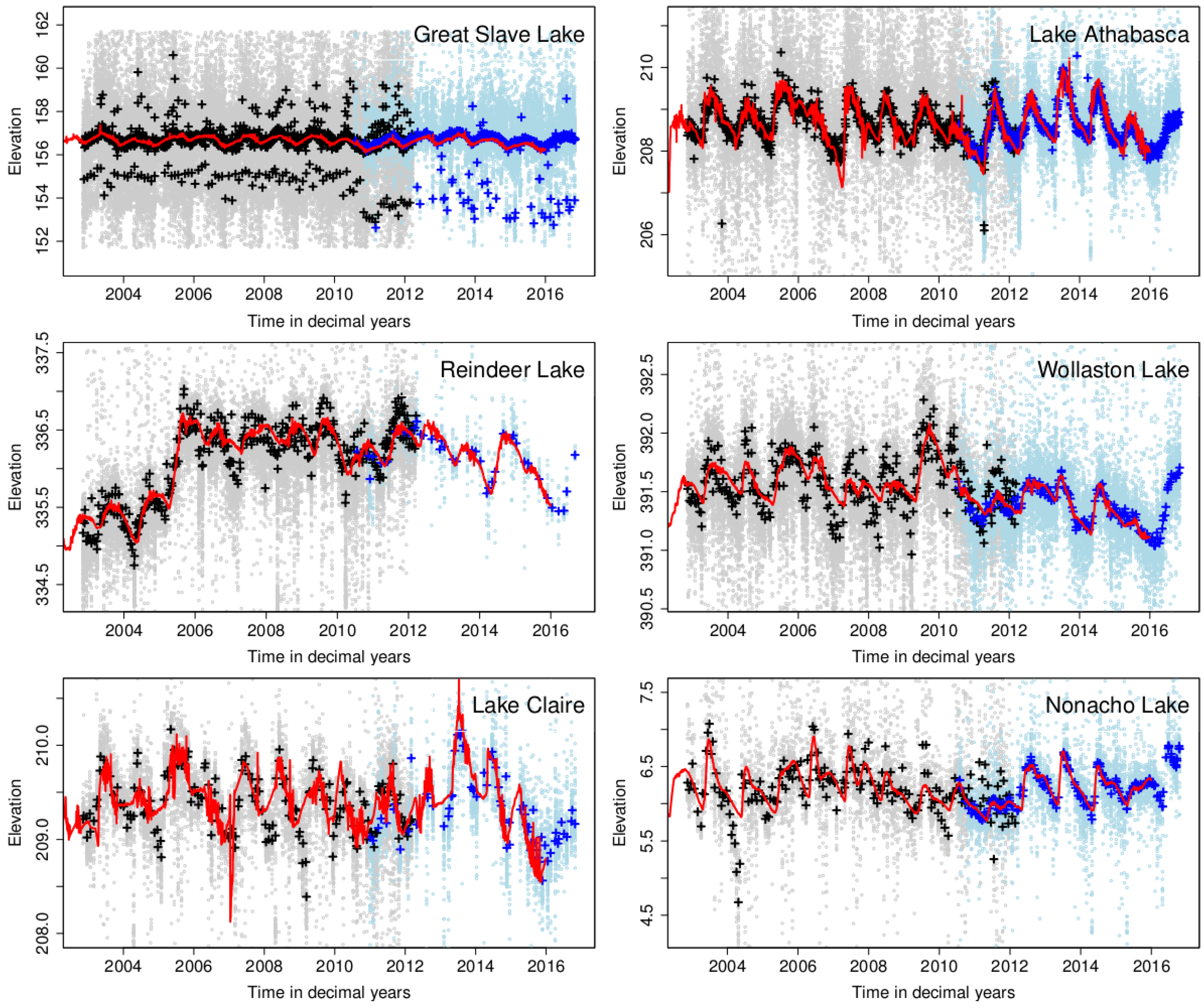
Figure 7.
(A) the WGS84 elevations for the Danish lakes based on laser scanner data, CryoSat-2 and Envisat; (B) the ratio [Envisat/CryoSat-2] of the standard deviation of the estimated mean water level.
Figure 7.
(A) the WGS84 elevations for the Danish lakes based on laser scanner data, CryoSat-2 and Envisat; (B) the ratio [Envisat/CryoSat-2] of the standard deviation of the estimated mean water level.

Figure 8.
The water level time series of Great Slave Lake between January 2012 and May 2012. The gray (Envisat) and blue (CryoSat-2) circles represent the raw retracked water levels. The black (Envisat) and blue (CryoSat-2) crosses represent the predicted water level, and the red line is the in situ water levels.

Table 1.
RMSE values for CryoSat-2 and Envisat.
| Lake | RMSE CryoSat [m] | RMSE Envisat [m] | Area [] |
|---|---|---|---|
| Great Slave | 0.68 | 0.54 | 27,816 |
| Athabasca | 0.19 | 0.25 | 7782 |
| Reindeer | 0.12 | 0.19 | 5597 |
| Wollaston | 0.05 | 0.17 | 2272 |
| Claire | 0.20 | 0.23 | 1326 |
| Nonacho | 0.06 | 0.24 | 847 |
Table 2.
Heights in meter above WGS84 for selected Danish lakes.
| Lake | Laser | CryoSat-2 Height | CryoSat-2, sd | Envisat, Height | Envisat, sd | Area [] |
|---|---|---|---|---|---|---|
| Arresø | 40.41 | 40.10 | 0.004 | 39.67 | 0.009 | 39.67 |
| Mossø | 62.34 | 62.22 | 0.008 | 62.41 | 0.039 | 16.34 |
| Skanderborgsø | 63.01 | 62.82 | 0.008 | 63.12 | 0.030 | 8.67 |
| Juelsø | 60.91 | 60.75 | 0.011 | 60.38 | 0.025 | 8.43 |
| Tystrup Sydsø | 44.43 | 44.07 | 0.009 | 44.55 | 0.165 | 6.73 |
| Gyrstinge Sø | 58.20 | 59.94 | 0.011 | 60.53 | 0.021 | 2.04 |
| Fårup Sø | 88.17 | 126.18 | 0.053 | 133.44 | 0.714 | 0.96 |
© 2017 by the authors. Licensee MDPI, Basel, Switzerland. This article is an open access article distributed under the terms and conditions of the Creative Commons Attribution (CC BY) license (http://creativecommons.org/licenses/by/4.0/).
Share and Cite
MDPI and ACS Style
Nielsen, K.; Stenseng, L.; Andersen, O.B.; Knudsen, P. The Performance and Potentials of the CryoSat-2 SAR and SARIn Modes for Lake Level Estimation. Water 2017, 9, 374. https://doi.org/10.3390/w9060374
AMA Style
Nielsen K, Stenseng L, Andersen OB, Knudsen P. The Performance and Potentials of the CryoSat-2 SAR and SARIn Modes for Lake Level Estimation. Water. 2017; 9(6):374. https://doi.org/10.3390/w9060374
Chicago/Turabian StyleNielsen, Karina, Lars Stenseng, Ole Baltazar Andersen, and Per Knudsen. 2017. "The Performance and Potentials of the CryoSat-2 SAR and SARIn Modes for Lake Level Estimation" Water 9, no. 6: 374. https://doi.org/10.3390/w9060374
Note that from the first issue of 2016, this journal uses article numbers instead of page numbers. See further details here.