
Evaluation of the SMOS-Derived Soil Water Deficit Index as Agricultural Drought Index in Northeast of Brazil


1
Department of Civil Engineering, University of the Western Plains ‘Ezequiel Zamora’, San Carlos Campus, San Carlos 2201, Venezuela
2
Laboratório de Analise e Processamento de Imagens de Satélites, Instituto de Ciências Atmosféricas, Universidade Federal de Alagoas, A. C. Simões Campus, Maceió 57072-970, Brazil
*
Author to whom correspondence should be addressed.
Water 2017, 9(6), 377; https://doi.org/10.3390/w9060377
Submission received: 13 March 2017
/
Revised: 27 April 2017
/
Accepted: 24 May 2017
/
Published: 27 May 2017
(This article belongs to the Special Issue Drought Monitoring, Forecasting, and Risk Assessment)
Abstract
:Northeast Brazil (NEB) has recently experienced one of its worst droughts in the last decades, with large losses on rainfed agriculture. Soil moisture is the main variable to monitor agricultural drought. The remote sensing approach for drought monitoring has been enriched with the launch of the Soil Moisture and Ocean Salinity (SMOS) in November 2009 by European Space Agency (ESA). In this work, the Soil Water Deficit Index (SWDI) was calculated using the SMOS L2 soil moisture in the NEB. The SMOS-derived SWDI data (SWDIS) were evaluated against the atmospheric water deficit (AWD) calculated from in situ observations. Comparisons were made at seven-day and 0.25° scales, over the time-span of June 2010 to December 2013. It was found that the SWDIS has a reasonably good overall performance in terms of the drought-weeks detection (skill = 0.986) and capture of the upper soil moisture temporal dynamic (r = 0.652), implying that the SWDIS could be used to track agricultural droughts. Furthermore, SWDIS shows poor performance at sites located in mountains regions affected by severe droughts (−0.10 ≤ r ≤ 0.10). It is also noted that the vegetal cover/use, climate regime, and soil texture have little influence on the AWD-SWDIS coupling.
1. Introduction
Climate variability and extreme weather events threaten many populations throughout the world [1]. The evidence indicates that, in many of these regions, variability and extreme events are increasing [2,3]. In recent years, droughts have received a special attention in Brazil, because they have been experienced with higher frequency, spatial extent, severity, and duration [4,5]. Some studies have also revealed that prolonged droughts and increased evaporation can lead to reduced water supply, crop failure, and diminished power generation, causing dramatic societal effects such as water rationing and massive electricity blackouts [4,6,7,8].
Although most regions of Brazil have suffered extreme droughts, their impacts are significantly more complex in the semiarid region of Northeast Brazil (NEB) due to its high variability of precipitation in both time and space [8,9,10]. It is also the world’s most densely populous dry land region [11,12,13]. Historically, NEB has been hit by many droughts. However, the 2012/2015 drought was one of the most severe in the recent decades with more than 10 million people affected in the semi-arid region [14]. This extreme condition in the northeast was linked to the deficit of rainfall and drying conditions that contributed to reduced soil water availability [15,16].
The majority of smallholder farmers living in NEB rely on subsistence agriculture, therefore droughts often trigger water shortage, leading to crop and economic losses [11,17,18]. Different types of drought are recognized in the world, including meteorological, agricultural, and hydrological drought, depending on the variable used to characterize this natural hazard and its spatial and temporal scale [19,20]. Unlike other types of droughts, the agricultural drought has a direct impact on rainfed-based agricultural production [21]. Usually, an agricultural drought is considered to begin when the soil moisture availability to plants drops to such a level that it unfavorably affects the crop yield and therefore agricultural production [22,23].
As already mentioned, droughts are the main cause of limited productivity of rainfed agriculture in NEB [24,25]. Hence, assessment of agricultural drought has a primary importance for rainfed agriculture planning and management. Several drought indices based on combination measures of precipitation, temperature and soil moisture, have been derived in recent decades to assess the effects of agricultural droughts and besides measure their intensity, duration, severity and spatial extent [26,27]. Among these, the Crop Moisture Index (CMI; Palmer, 1968), Atmospheric Water Deficit (AWD; [28]), Soil Moisture Index (SMI; [29]), Agricultural Reference Index for Drought (ARID; [30]), and Soil Water Deficit Index (SWDI; [22]) are the most widely used for monitoring drought conditions on extensive crops (e.g., cereals).
The amount of available soil moisture in the root zone is a more critical factor for crop growth than the amount of precipitation deficit or excess. In fact, the soil moisture deficit in the root zone during various stages of the crop growth cycle has a profound impact on the crop yield [31]; therefore, the accurate knowledge of soil moisture is a key aspect for the characterization of agricultural droughts. Ground-based soil moisture measurements are very accurate, but they have an application limited because of their point-based nature, their reduced spatial extent, and the high variability of soils [27]. Nevertheless, that limitation has been gradually overcome due to progress in the development of satellite technology and retrieval algorithms for quantifying soil moisture from active and passive microwave satellite platforms [32,33,34]. Currently, these estimates are used to detect and monitor regions affected by droughts and have the advantage of their wide spatial distribution and coverage, as well as the temporal availability of data [35,36,37,38,39].
The remote sensing approach for drought monitoring has been enriched with the launch of new missions dedicated to global surface soil moisture (SSM) monitoring. For instance, the Soil Moisture and Ocean Salinity (SMOS) satellite launched in early November 2009 by European Space Agency (ESA), and the Soil Moisture Active Passive (SMAP) satellite launched in January 2015 by National Aeronautics and Space Administration (NASA). SMOS is an L-band passive microwave satellite that measures brightness temperatures with Microwave Imaging Radiometer using Aperture Synthesis (MIRAS) [35,40].
SMOS is opening new perspectives for monitoring the effects of agricultural droughts over large agricultural regions [35,36,41]. In this sense, some recent studies have proposed new indices based on soil moisture estimates derived from SMOS to assess agricultural drought. Scaini et al. [37] demonstrated the feasibility of SMOS-derived soil moisture anomalies for determining drought conditions in a central semiarid sector of the Duero basin in Spain. In this same region, Martínez-Fernández et al. [36] compared series of the SWDI calculated with SMOS L2 data with ones obtained from in situ soil moisture data, and their results showed that SMOS-derived SWDI reproduces well the soil water balance dynamic. More recently, Sánchez et al. [42] introduced a new index, so-called the Soil Moisture Agricultural Drought Index (SMADI), which is a synergistic fusion of the SMOS L2 soil moisture with the Moderate Resolution Imaging Spectroradiometer (MODIS)-derived land surface temperature (LST) and several water/vegetation indices for agricultural drought monitoring. These authors demonstrated that SMADI could provide early warning of incipient drought impacts in rainfed farming systems.
Despite the great potential of SMOS for agricultural drought monitoring, very few works have been published using soil moisture derived from SMOS data in worldwide; especially in Brazil. For instance, Rossato and Angelis [43] used data of brightness temperature sensor MIRAS aboard the SMOS satellite to assess the pattern of soil moisture in densely vegetated areas in some Brazilian locations with soil moisture data measured in situ. They have reported that the SMOS-derived data infer accurate values of soil moisture over those areas, which demonstrated the feasibility of SMOS to support in planning for planting and/or irrigation of crops. Over NEB, Ferreira et al. [44] found that the soil moisture changes estimated by a Model of Soil Moisture for Agricultural Activities (MUSAG) and those derived from SMOS show a significant correlation for 184 selected sites within the Ceará state. Their results indicated that SMOS data might represent the soil moisture change in the Brazilian Caatinga satisfactorily, allowing assessment of the seasonality of the water balance in this region.
In this work, the focus is specifically on the entire NEB, which has been hit by an unprecedented drought since 2012. Severe droughts have caused serious impacts on water supply and agriculture of the NEB, especially during the rainy season [8,15,45]. The main goal of this work is to compare the series of the SWDI calculated with SMOS L2 data with those of the Atmospheric Water Deficit derived from in situ observations, which is used as a reference index. We also analyzed its feasibility for large-scale agricultural drought monitoring. It is important highlight that in none of previous study has been examined the SMOS-derived SWDI as a proxy of upper soil moisture in the NEB.
2. Materials and Methods
2.1. Study Area
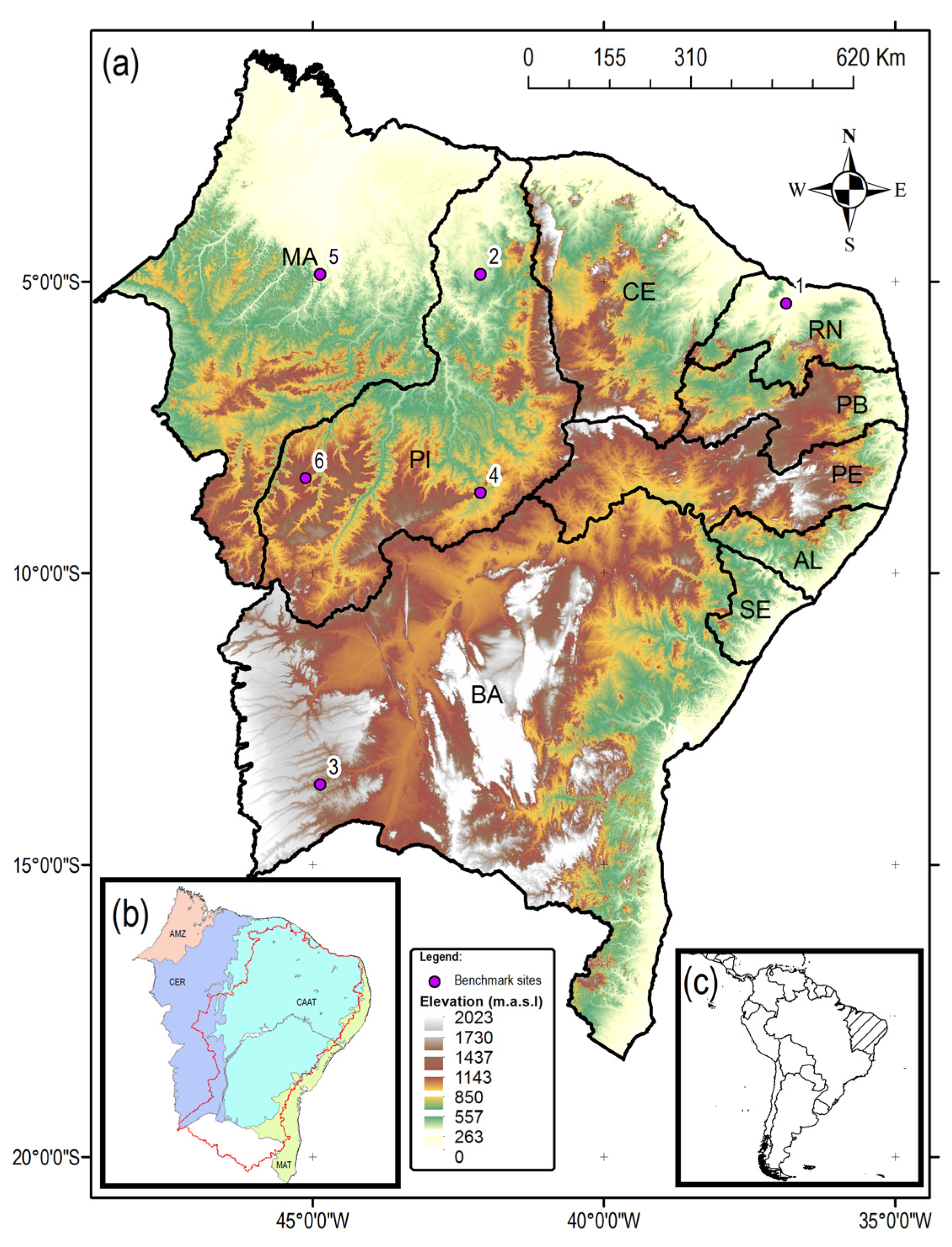
Northeast Brazil (NEB) is located within 1.3°–18.2° S and 34.4°–48.4° W (Figure 1), occupying an area of about 1,555,000 km2 (nearly 19% of Brazilian territory). It is divided into nine federal states: Maranhão (MA), Piauí (PI), Ceará (CE), Rio Grande do Norte (RN), Paraíba (PA), Pernambuco (PE), Alagoas (AL), Sergipe (SE) and Bahia (BA), which cover roughly 21%, 16%, 10%, 3%, 4%, 6%, 2%, 1% and 36% of NEB, respectively. NEB has more than 53 million inhabitants (about 30% of the Brazilian population) and a human population density of about 34 inhabitants per square kilometer [13], of which about 50% are considered poor by Brazilian standards [46]. Its climate is hot (annual mean: 12–40 °C) and characterized by annual precipitation in amounts ranging between 250 and 2000 mm. The rainy season occurs at different times of the year for different sub-regions. The eastern part of NEB has its rainy season between May and August. The southern part of the region has maximum precipitation in November–December. The semi-arid northern part of NEB has its rainy season between February and May [11,16,47]. The Inter Tropical Convergence Zone (ITCZ) controls the weather system in most of the NEB. When the ITCZ reaches its southernmost position in the course of the year, it induces the production of rainfall over almost the entire NEB. The Upper Tropospheric Cyclonic Vortex, Easterly Waves Disturbances, and Squall Lines also cause heavy rainfall at any time of the year. The south of Bahia state has actuation of the Front Systems and the South Atlantic Convergence Zone [12,17]. Rainfall in NEB shows a high interannual and seasonal variability, which favors the occurrence of prolonged droughts [48].
The agricultural census from Instituto Brasileiro de Geografia e Estatística (IBGE) for the reference year 2006 showed that the states BA, PE and PI group about 27%, 21% and 18% of the croplands, respectively (mainly sugarcane and cotton), whereas BA, MA and CE congregate about 40%, 19% and 9% of pasture areas, respectively [49]. For most rainfed crops of the NEB, the growing season occurs from February to May [50]. An internal portion of the NEB (~63%) is occupied by a semi-arid polygon known as the Sertão region (Figure 1b), where the subsistence agriculture is dominant and droughts are very frequent [8,51]; consequently, efficient management of the Sertão’s water resources is of extreme importance for socioeconomic development of this sub-region. The main biomes of NEB are Amazônia (Amazonia), Cerrado, Mata Atlântica (Atlantic Forest), and Caatinga, which cover about 7%, 29%, 10%, and 52% of the entire NEB, respectively (Figure 1b). The Caatinga biome is characterized by a mosaic of seasonally dry tropical forests and thorn scrubs, with more than 2000 species of vascular plants [52,53], commonly inappropriate for rainfed agriculture [51]. The biome Cerrado is a vast tropical savanna, whose main habitats are forest savanna, wooded savanna, park savanna, gramineous-woody savanna, savanna wetlands, and gallery forests [54]. The Mata Atlântica biome also is known as Atlantic Forest. It extends along the Atlantic coast of the NEB and groups the seasonal moist and dry broad-leaf tropical forests, tropical and subtropical grasslands, savannas, and shrublands, and mangrove forests [55]. The Amazônia biome is also known as Amazon Rainforest. It is a moist broadleaf forest, which comprises the largest and most biodiverse tract of tropical rainforest in the NEB [56]. On the other side, most of the soils of NEB are Neossolos with a high content of clay (nearly 40% or more) and a bulk density about 1.25 g cm−3 [57].
2.2. Datasets
2.2.1. In Situ Database
The temporal variations of the upper soil moisture are mainly driven by the variations of the atmospheric water deficit near to topsoil [22,37]. In order to verify the impact of droughts on the upper soil moisture of the NEB, daily values of the Atmospheric Water Deficit (AWD) were used. The calculation of the AWD require as inputs, observations of daily rainfall and daily potential evapotranspiration (ETo) [26]. For this study, four grids with a spatial resolution of 0.25°, of daily rainfall, ETo, maximum and, minimum temperature for the entire Brazil throughout the period of 1980 to 2013 was used. Xavier et al. [59] developed these grids using in situ observations, which were gridded using an inverse-distance weighted interpolation algorithm. The dataset is updated regularly, and it is freely available at http://careyking.com/data-download/. This dataset is chosen because it constitutes the most complete set of in situ climatic observations for the northeast Brazil [60]. Their data sources are the Instituto Nacional de Meteorologia (INMET), the Agência Nacional de Águas (ANA), and Departamento de Águas e Energia Elétrica de São Paulo (DAEE) [59]. More details about the distribution of weather station net on the NEB can be found in Xavier et al. [59]. Daily ETo was estimated using the Penman–Monteith methodology [61,62]. All grids were clipped using a shapefile of the NEB as a mask, resulting new grids with 2050 equally spaced nodes at about 28 km. Hereinafter, this is so-called the Reference Discrete Grid (RDG).
2.2.2. SMOS Database
MIRAS-SMOS is an interferometric radiometer that measures the thermal emission from the Earth in the 1.4-GHz protected frequency range in full-polarization and for incidence angles from 0° to about 60°. Microwave emissions from the Earth’s surface at L-band are attenuated by dielectric materials, therefore these attenuation patterns are used to estimate soil moisture for the first 5 cm of soil. SMOS has a revisit time of 3 days at Equator, an accuracy of 4% volumetric soil moisture and a native spatial resolution of about 35–50 km [63,64].
In this study, the SMOS Soil Moisture Level 2 User Data Product version 6.20 was used to estimate the upper soil moisture in the NEB (for details on SMOS L2, we recommend the work of Kerr et al. [65]). This product is disseminated through ESA [66], over the Icosahedral Snyder Equal Area Earth grid with equally spaced nodes at about 15 km, known as the Discrete Global Grid (DGG). Additionally, the daily SMOS L2 soil moisture data are available from January 2010 to the present. Since the rainfall and Eto datasets end in December 2013, the time-span from January 2010 to December 2013 was chosen as analysis period. The first semester of 2010 was omitted, because of the MIRAS instrument underwent several tests.
The SMUDP2 product provides to users the retrieved surface geophysical parameters as well as quality indicators. The soil moisture retrieval is associated with a Data Quality Index (DQX), which represents the uncertainty of the retrieval [36]. In this research, two filters were applied to obtain reliable SMOS soil moisture retrievals: (1) SMOS retrievals with DQX less than 0.04 m3 m−3; and (2) SMOS retrievals without significant radio frequency interferences (RFI); that is, SMOS SM data with a RFI probability higher than 20% were filtered out. These criteria were implemented to the ascending and descending orbits separately, and later, the average of the two orbits for each day was calculated. Similar to rainfall and ETo, the filtered SMOS product was clipped to match the spatial extent of the NEB, resulting a grid with 9205 equally spaced nodes at about 15 km.
2.3. Methodology
2.3.1. SMOS-Derived Soil Water Deficit Index (SWDIS)
The Soil Water Deficit Index (SWDI) was proposed by Martínez-Fernández et al. [22] in order to characterize the agricultural drought based on in situ soil moisture series and basic soil water parameters. The SWDI was formulated as follows:
where θ is the soil water content, FC denotes field capacity and AWC available water content, which is the difference between FC and WP (wilting point). Authors argue that when the soil reaches a water content below θFC, the deficit begins and water stress could occur. Even though soil water just below field capacity not always triggers a plant water stress, below that point, plants are no longer in optimal conditions as they start to need to use more and more energy for water uptake. The concept of the readily available soil water (RAW) of the FAO (Food and Agriculture Organization) guidelines for the determination of the crop water requirements is similar [62]. In fact, the p factor of the RAW definition is the average fraction of total available soil water (TAW) that can be depleted from the root zone before moisture stress occurs [36,61,62].
Taking into account that the p factor varies for the main crops from 0.2 to 0.8 and, that 50% of the crops considered by Allen et al. [62] has a p factor below 0.5, Martínez-Fernández et al. [22] developed a severity scale for the SWDI. Thus, a positive SWDI value reveals an excess of water in the soil; when it equals zero, the soil is at the field capacity (i.e., no water deficit and no drought). Negative values indicate agricultural drought, and its impact will depend of the type of crop and the fraction of total available soil water that can be depleted from the root zone before moisture stress occurs [36,62]. When the SWDI ≤ −10, the water deficit is absolute; that is, the soil water content is below the lower limit of available water for plants [22].
The use of the SWDI in large-scale agriculture applications needs to know the spatial distribution of the parameters FC and WP in the areas under study. This is a critical issue in the NEB, because there is not enough available information about these soil water parameters. For those areas where specific information on soil water parameters is scarce or absent, some researchers have proposed different approaches for estimating FC and WP based on SMOS L2 soil moisture. Recently, Martínez-Fernández et al. [36] found that the SWDI at a weekly time scale, based on the percentile method developed by Hunt et al. [29], where the 5th percentile is used as an estimator of WP and the 95th percentile as an estimator of FC, shows good correlation with the SWDI calculated with in situ data. In this line, for this study, the 5th and 95th percentiles were used as estimators of WP and FC, respectively at every DGG. Both parameters were derived from the SMOS L2 soil moisture series for the period June 2010–December 2013.
The daily SMOS-derived SWDI data (i.e., 9205 SMOS grid cells for each day within the NEB, see Section 2.2.1) were re-sampled with the nearest neighbor interpolation technique to a resolution of 0.25° to ensure consistency with the rainfall and ETo data. This procedure allowed the use of a common grid for the daily SMOS soil moisture, daily rainfall, and daily ETo, whose nodes coincide with those from the RDG (see Section 2.2.1). Next, the daily SMOS-derived SWDI data were weekly averaged (SWDIS) at every RDG (with the arithmetic mean). When, within a RDG, there were less than three daily data during the week, the weekly SWDIS average was omitted (i.e., these were considered as missing values). This temporal scale was chosen because farmers commonly use a weekly period for irrigation schedules. The number of weeks was based on International Organization for Standardization (ISO) standard week numbers.
2.3.2. Atmospheric Water Deficit Derived from in Situ Observations (AWD)
The concept of the Atmospheric Water Deficit (AWD) was proposed by Purcell et al. [28]. AWD is a suitable tool to identify the drought dynamics related to soil water storage [26,67]. For its calculation, the cumulative ETo for the preceding 6-day and the day under consideration are summed (7-day total), and the 7-day cumulative precipitation is subtracted from this value, resulting in a 7-day cumulative AWD estimate for each day of the long-term record.
In the present work, a modified AWD suggested by Martínez-Fernández et al. [36] was used, where the AWD is calculated as the 7-day running sum of precipitation minus the 7-day running sum of ETo to obtain negative values, similar to those of the SWDI, during the dry episodes. The SWDIS was then compared with the AWD for the common period, using a weekly temporal scale as previously described (i.e., June 2010–December 2013, equivalent to 186 weeks).
2.3.3. Linear Relationship and Drought-Weeks Probability of Detection (POD)
It is worth be mentioned that the upper soil moisture is closely linked to atmospheric water deficit [26,36,67]. For this reason, a linear correlation analysis can be used to explore the temporal relationship between both signals. Hence, the Pearson's correlation coefficient (r) was used to quantify the strength of the relationships between the SWDIS and ADW time series at pixel scale, whereas its statistical significance was tested on base to the Student’s t-test [68]. To guarantee the reliability of the comparison, those cases where the number of SWDIS-ADW pairs was less than 30 were omitted [69]. This threshold was changed to 10, when the growing season was analyzed (i.e., from February to May).
The drought-weeks detection capability based on the SWDIS is important for irrigation schedules. This term refer to the skill of the SWDIS for detection of drought weeks, taking into account a threshold to differentiate the non-drought weeks from drought-weeks. In assessing the SWDIS performance for detection of drought weeks on each RDG grid cell, the Probability of Detection (POD) was used [47,70]. The POD indicates the fraction of the observed drought weeks that were correctly detected; with a threshold equal zero for SWDIS and AWD. The perfect score for this metric is one. POD is given by:
where A and C represent number of hits and number of misses for pairs of SWDIS-AWD, respectively.
3. Results
3.1. Spatial and Seasonal Relationship between the SWDIS and AWD
Following the computation of SWDIS and ADW (Section 2.3), a point-to-point comparison was carried out to explore the overall association between both variables. The SWDIS-AWD pairs for the entire NEB covering the period of June 2010 to December 2013 (i.e., 186 weeks of time span) is shown in Figure 2a, whereas Figure 2b displays only those pairs during the growing season (i.e., February to May for each year, equal to 12 weeks). In both cases, the SWDIS showed a moderate overestimation of the observed values of AWD ≤ 0, though it tends to underestimate positive values.
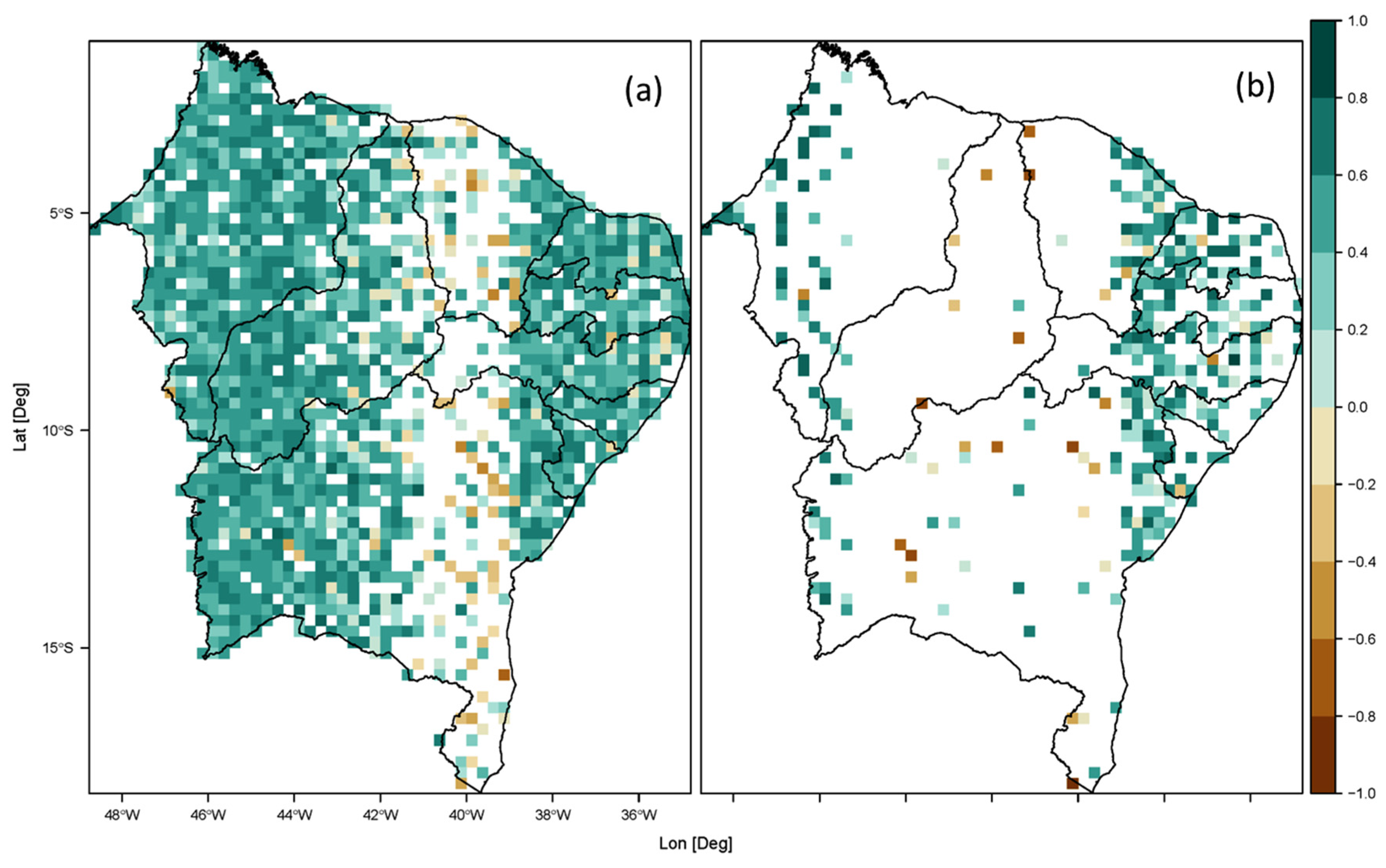
In order to evaluate the effect of spatial factor on the SWDIS-AWD relationship, a linear correlation analysis was applied at each grid point (0.25° × 0.25°). The Pearson’s correlation coefficient is non-dimensional and quantifies the strength and direction of the linear association between both variables over time. Figure 3a shows the spatial distribution of linear correlation between the SWDIS and AWD for the entire year. Pearson’s correlation coefficients were slightly high in most of the RDG grid cells (averaged r for all RDGs, 0.652). At first view, the SWDIS captures reasonably well the spatial variability of the AWD, mainly over the major part of MA and PI (Figure 1). On the other hand, this relationship stayed moderately high throughout the growing season (averaged r for all RDGs, 0.633), which was reflected by values of correlation similar to those seen for the entire year (Figure 3b).
An aspect less evident in Figure 3 is the presence of zones where the SWDIS-AWD relationship was significantly weak (i.e., r near to zero) or even negative. This asynchronous relationship was more marked throughout the growing season and over some croplands located in PI and BA (Figure 1 and Figure 3b). It is also possible to see that this discrepancy was significantly frequent inside the central Sertão region (in particular, between 40° and 45° west longitude). An analysis more exhaustive of the results revealed that when the number of valid SWDIS-AWD pairs increases in RDG grid cells, the linear correlation tends to be stronger (not shown). However, this last feature cannot be generalized to the entire NEB, due to that it was only observed in certain grid points.
3.2. The Skill of SWIDS in Terms of Detection of Drought Weeks
In order to improve the assessment of the performance of the SWDIS was calculated the POD on each RDG grid cell. This metric shows how many drought weeks were correctly identified by the SWDIS. For this analysis, it was assumed that a drought week occurs when AWD < 0 and SWDIS < 0, as in Martínez-Fernández et al. [36]. A yearly average POD equal to 0.986, and an average POD for the growing season of 0.995 were obtained (Figure 4), indicating that the drought periods were well captured by the SWDIS. However, Figure 3 and Figure 4 reveal a high proportion of gaps for the AWD-SWDIS linear correlation and POD from 37° to 41° longitude. This behavior was caused mainly by radio frequency interference during the most of the study period. In general, an increase in the radio frequency interference increase the values flagged as poor quality in the SMUDP2 product (i.e., RFI_Prob field ≥ 20%), leading to a very little amount of daily SMOS L2 soil moisture data available for this region.
3.3. Behavior of the SWDIS-AWD Relationship at Local Scale
In order to examine with more detail the SWDIS-AWD relationship at local scale, 6 RDG grid cells were selected as benchmark sites (Figure 1). Sites were chosen based on proportion of complete pairwise. Thus, it was taken into account a threshold of 80% (i.e., N ≥ 149 weeks). Table 1 shows the geographical location of the benchamark sites and other features such as their elevation above sea level, soil texture, soil taxonomy, biome, and soil cover/use. Ultisols are the dominant soils with the exception of Oxisol soil present at Correntina. On the other hand, Carnaubais croplands are mainly dedicated to cotton and banana crops; whereas at Fazendas do Piauí large monocultures of soya and cotton are dominant. Carnaubais and Campo Maior are located in a vast open flatland. Otherwise, Correntina and Fazendas do Piauí are located in high mountains with complex relief (Figure 1).
A Walter–Lieth climatic diagram [73] at each benchmark site was used to characterize the climate regime over the period of 1980–2013 (Figure 5). The mean precipitation, mean maximum daily temperature, mean minimum daily temperature, and absolute monthly minimum temperature were derived from climatic datasets developed by Xavier et al. [59]. In principle, Carnaubais (P = 623 mm/year) and São Raimundo Nonato (P = 669 mm/year) show semiarid climate regimes characterized by the presence of a short rainy season from January to March (i.e., weeks: 1–17). Both locations are within the Sertão region (Figure 1b), which is the driest of the NEB [13,45,74]. In contrast, climatic diagrams for Campo Maior (P = 1300 mm/year) and Esperantinópolis (P = 1378 mm/year) reveal a longer wet period (i.e., December–May, Weeks 1–22, and 48–52), where monthly precipitation is greater than 100 mm. Besides, in spite of show less amount of yearly precipitation, Correntina (P = 1009 mm/year) and Fazendas do Piauí (P = 1202 mm/year) have the most long wet period (i.e., October–April; weeks: 1–17, and 40–52).
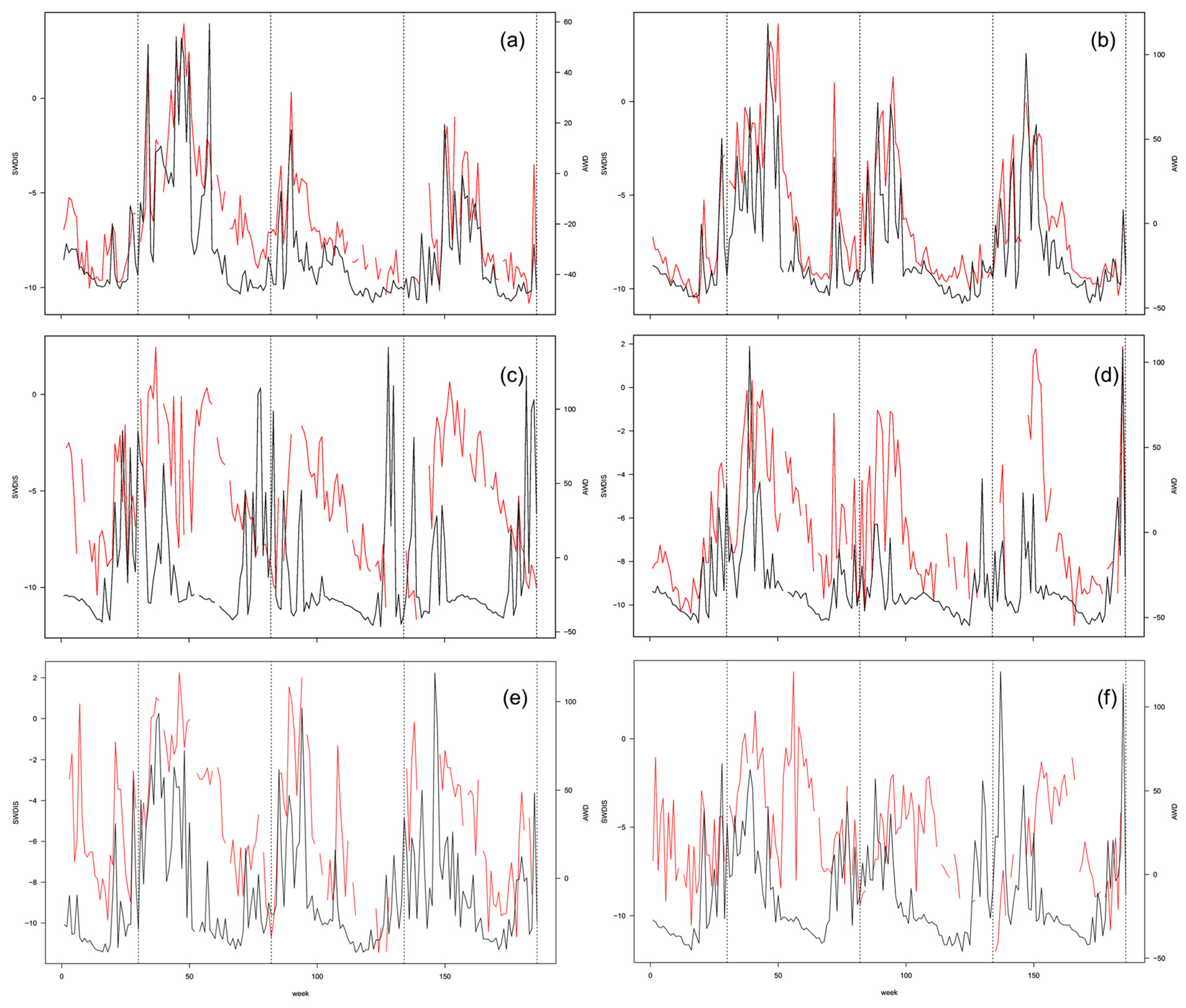
Figure 6 shows a visual comparison of the SWDIS and AWD time series at each site. Note that the SWDIS had highest capacity to capture the temporal dynamic of the drought at Carnaubais (r = 0.85; Figure 6a) and Campo Maior (r = 0.85; Figure 6b). Furthermore, the drought periods were well captured by the SWDIS (POD = 1.00 for both cases), revealing a strong linear coupling between the superficial soil moisture and environmental dryness. On the other hand, the AWD-SWDIS relationship was weaker in Fazendas do Piauí (r = 0.02; Figure 6f) and Correntina (r = −0.108; Figure 6c), whereas at São Raimundo Nonato (r = 0.578; Figure 6d) and Esperantinópolis (r = 0.640; Figure 6e) a slightly improvement was observed. At first view, this result suggests that the climate regime does not affect the overall performance of the SWDIS, when it is used in order to track the local drought dynamic (based on the AWD).
When the inter-week variation calculated by successive differences from the SWDIS data was compared to those derived from the AWD data in each benchmark site, some consecutive weeks where the values of the AWD tend to stay almost constant and persistently negative during several weeks were observed. This feature was only noted in Fazendas do Piauí, Correntina, and São Raimundo Nonato (not shown). In these sites, the SWDIS seems to vary uncoupled to the AWD, but showing negative values (see Figure 6c,d,f); in particular, through weeks: 51–60, 106–123, and 152–163. In order to investigate the effect of the duration of dry spells on the AWD-SWDIS coupling at Fazendas do Piauí, Correntina, and São Raimundo Nonato, the amount of dry episodes with AWD ≤ −20 and length ≥ 4 weeks was calculated. For these locations, results show the occurrence of four, nine and nine dry episodes with an average duration of 28, 25, 11.22, and 14.4 weeks, respectively. Overall, the persistence of dry spells seems to affect the performance of the SWDIS. That is, an increase in the persistence of drought environmental conditions tends to weaken the coupling between the AWD and SWDIS; in particular, at Fazendas do Piauí.
In order to assess if there is a delay between the signals of SWDIS and AWD a cross-correlation analysis was applied in each benchmark site. This analysis computes the linear correlation between AWD [t + k] and SWDIS [t], where t represents number of weeks and k indicates the lag value between the SWDIS and AWD, respectively. It was found that the AWD-SWDIS connection is persistent until by 6 weeks, but with weaker in strength than when k = 0 (i.e., both signals in phase) at Carnaubais, Campo Maior, São Raimundo Nonato, and Esperantinópolis. In contrast, a decoupling very evident was found for values of k from 0 to 6 weeks at Correntina and Fazendas do Piauí (not shown). These results reveal an important disconection between the dynamics of the atmospheric system and the soil system at Correntina and Fazendas do Piauí, which seems to be driven by environmental conditions.
Some statistical parameters of the SWDIS and AWD at benchmark sites are shown in Table 2. It is possible to see that the cropland and pasture covers show notable differences in terms of their correlation coefficients. The most obvious dissimilarity is evident when are compared Carnaubais and Fazendas do Piauí (Id = 1 and 6). Despite their different correlation coefficient (r = 0.85 and 0.02, respectively), these sites coincide with the dominant soil use (i.e., cropland). The situation is similar when comparing Campo Maior (r = 0.85; soil cover: pasture) with Correntina (r = −0.11; soil cover: pasture), suggesting that the soil cover/use had little influence on the AWD-SWDIS relationship.
To get further insight into the characteristics of the precipitation during the analyzed period (i.e., 2010–2013), it was compared to 1980–2013 and 2010–2013 precipitation average (see Figure 5 and Table 2). Results revealed that most of the benchmark sites were exposed to drought conditions. For example, the annual average precipitation for the 2010–2013 period at São Raimundo Nonato, Carnaubais, Campo Maior, and Esperantinópolis was −22%, −17%, −15%, and −5%, respectively with respect to their observed average through the 1980–2010 period. It is noteworthy that the spatial distribution of these sites in Figure 1, suggests the occurrence of a severe drought mainly focused in the Sertão region. As expected, this result is coherent with the long dry spells previously identified at São Raimundo Nonato.
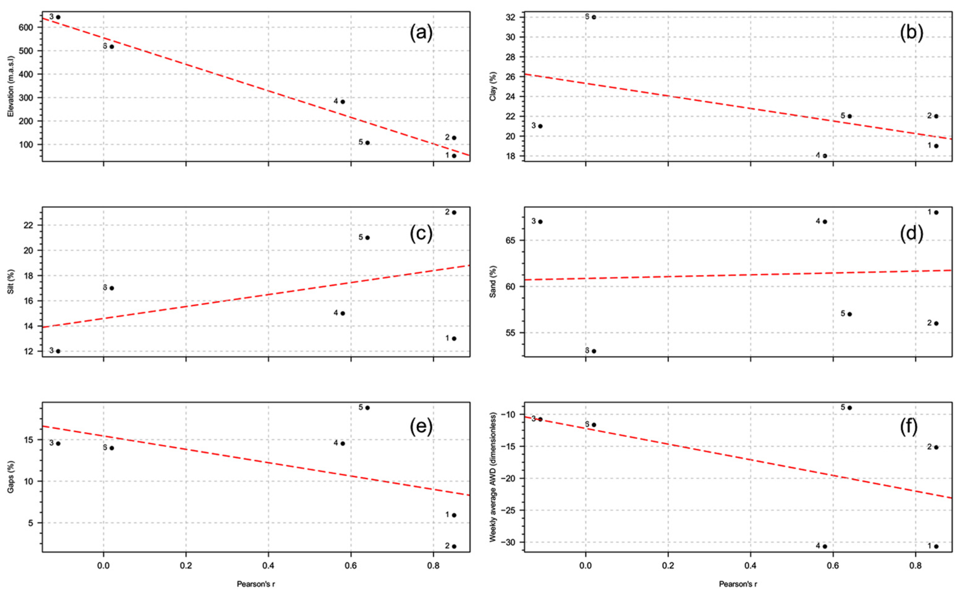
Finally, in order to assess if the SWDIS-AWD relationship is sensitive to the texture of the soil, elevation, gaps in the SWDIS-AWD pairs, and environmental dryness, a correlation analysis was applied considering the values of percentage of clay, sand and silt shown in Table 1 against the Pearson correlation coefficient (r) from Table 2. Figure 7 displays a summary of the comparisons. Paired values of clay-r (Figure 7b), silt-r (Figure 7c), and sand-r (Figure 7d) showed linear correlation coefficients equals to −0.53, 0.45, and 0.06, respectively. At first view, a low clay content and high silt content seems to be favorable for the SWDIS-AWD coupling (at least, at Campo Maior and Esperantinópolis). However, they were statistically not significant at the 5% level, implying that the texture of the soils is not associated necessarily with the soil–atmosphere coupling in the entire NEB. On the other side, it is important to notice the strong association between the elevation and the SWDIS-AWD coupling (r = −0.97; p ≤ 0.05), suggesting that the SWDIS-AWD coupling could be mainly driven by topographical factors. In general, the SWDIS tends to show best performance as an agricultural drought index in open flatland (e.g., Carnaubais) than at mountainous regions (e.g., Correntina). Contrastingly, the percentage of gaps in SWDIS-AWD pairs and the intensity of drought based on weekly AWD did not affect significantly the overall performance of the SWDIS at benchmark sites (r = −0.53 and −0.51; both with p > 0.10).
4. Discussion
In line with the results from some previous studies [26,28,36,67,75,76], it was found that the atmospheric conditions over NEB influences the upper soil water balance dynamic. This characteristic is reflected by a moderate coupling strength between the AWD and SWDIS from June 2010 to December 2013 in the entire NEB (Figure 2 and Figure 3). There, it was also possible to identify different levels of bias between both signals. As expected, the AWD cannot be directly compared to the SWDIS, as the variation range of the first was larger (−59 ≤ AWD ≤ 406) than that of the second (−16 ≤ SWDIS ≤ 52) (Figure 2a). Consequently, one could expect that a negative value of the AWD will be reflected by a negative SWDIS value, but with lower magnitude.
Results revealed that during the 2012–2015 drought the central Sertão region was exposed to drought conditions more severe than other regions of the NEB, which is consistent with find by [13,14,15,45]. It is interesting to indicate that the Sertão region showed high radio frequency interference (RFI) during the analyzed period, leading to SWDIS time series with high proportion of gaps. On the other side, according to Hengl et al. [72], various zones of the Sertão region have argillic horizons very near the surface, which could have favored the soil water retention in surface soil layer during the occurrence of a drought episode. Both physical factors could be related to the poor performance of the SWDIS in some areas of the Sertão region (Figure 3).
In terms of detection of drought weeks, the SWIDS showed a moderately high skill (Figure 4). One implication of this result is that there is great potential in using SWDIS to monitor weekly dry spells. The same conclusion was arrived at by Martínez-Fernández et al. [36], who found that the drought periods are relatively well captured by the SWDIS at the central part of Spain, which has a similar climatic regime to the NEB (Figure 5) [77].
Other relevant aspects were observed at the local scale. For instance, according to Hengl et al. [72], Carnaubais and Campo Maior, where the SWDIS-AWD relationship was stronger (Figure 6a,b), show Ultisols with a water table near the surface for much of the year (Table 1). Furthermore, Correntina and Fazendas do Piauí, where the SWDIS-AWD relationship was weaker (Figure 6c,d), present Oxisols and Ultisols, respectively, as their dominant soils (Table 1). It is well known that the amount of clay and sand has an important influence on the soil water dynamic [22]. In fact, soil water retention is strongly correlated to the clay content [78]. In this context, one could suppose that clay soils may show positive values of SWDIS, in spite of the presence of severe drought conditions (i.e., AWD << 0), leading to values of correlation near to zero or negative when the AWD and SWDIS are compared. About this point, results suggest that the AWD-SWDIS relationship was not influenced significantly by the soil texture. Evidence of this is that this physical attribute did not show a statistically significant correlation coefficient with respect to the AWD-SWDIS correlation when were taken into account all benchmark sites (Figure 7b–d). Nevertheless, caution must be taken about this hypothesis due to that the amount of benchmark sites represent less than 2% of the size of the sample (2050 RDG cells).
One of the advantages of SMOS is that it can observe at a lower frequency (1.4 GHz) than previous instruments (e.g., NASA/JAXA Advanced Scanning Microwave Radiometer (AMSR-E)) [79]. This frequency is less affected by the vegetation cover [64]. Moreover, the soil moisture retrievals on forest have been improved with the new level 2 V620 algorithm [80], which was the version used in this study. These features of SMOS help to explain why the influence of vegetal cover/use on the coupling strength between the AWD and SWDIS in the benchmark sites was little (see Table 1). However, despite this local response, results suggest that the SWDIS does not capture enough well the temporal dynamics of the agricultural drought in semiarid biomes such as in the Caatinga (Figure 3 and Figure 4). Previous studies have already shown that SMOS has a relatively low ability in arid and semiarid biomes [65,81], therefore, this result has been consistent.
A critical issue of soil moisture retrieval from SMOS is that their estimations are limited to the first centimeters of the surface soil layer (i.e., 0–5 cm) and depend on soil water content [36]. This water is stored not only in the surface layer but also in the root-zone layer [26]. Although some studies have demonstrated the presence of a strong correlation between the content of moisture in surface and root-zone [67,82], the coupling strength among soil layers decreases as depth increases, and moreover depend on the prevailing hydrometeorological conditions [36,83,84]. As already mentioned, the climatic conditions of the NEB during the period of analysis (i.e., June 2010–December 2013) were characterized by persistent drought conditions, which intensified near to end of 2012 and extended until 2015 [13,45,74]. It is convenient to mention that previous studies have indicated that the SMI–AWD relationship tend to be weaker in the drier years [29,85]. During the driest episodes, the atmospheric and soil dynamics are more disconnected, because the water transfer is mainly controlled by soil characteristics [22,86]. This physical feature would explain partially the AWD-SWDIS decoupling observed in sites such as São Raimundo Nonato (Figure 6d), where Marengo et al. [13] found the level of dryness most severe throughout the 2012–2015 drought. Note that this situation of extreme dryness can be observed in Figure 7f by the fact that the AWD was negative persistently at São Raimundo Nonato (see point # 4) over the time span of June 2010 to December 2013.
The physical factor that has more influence on the AWD-SWDIS coupling for the entire NEB is terrain elevation (Figure 7a). In general, the SWDIS shows better performance in open flatland than in areas with complex relief. The same behavior has previously been found for the retrieval of soil moisture from SMOS with respect to relief, and it has been attributed mainly to surface roughness [87,88].
Summarizing, the above results suggest that the topographical factors and the level of atmospheric dryness have played a key role in the overall performance of the SWDIS as a proxy for agriculture drought at local and regional scales. Overall, when the dryness level is persistently negative over time (i.e., AWD << 0) in mountain regions (e.g., Correntina), the SWDIS tends to show poor performance. On the other hand, the vegetal cover/use and soil texture are physical attributes that have a marked influence local, whereas that the RFI and biomes are dominant on the global performance of the SWDIS.
Although the results presented in this study are limited in terms of the time span of SWDIS (approximately four years), this index seems to be reliable when it is used to identify the beginning, end, and duration of a drought episode, because these attributes are inferred from the dry spells (i.e., drought weeks). However, the assessment of the SWDIS as a proxy of the superficial soil moisture deficit in the NEB should be further investigated by considering other agricultural drought indices obtained from in situ data, such as the Crop Moisture Index [89]. In any case, it should be pointed out that these preliminary results are very promising for the NEB, since in the future one could obtain the SWDI from exclusively SMOS data. The SWDIS could be also a suitable tool to monitor the drought dynamics related to soil water storage in open and low-elevation flatlands of NEB. In this context, its operative implementation may facilitate the preparation of drought plans by national government decision makers.
5. Conclusions
NEB suffers from regular droughts, particularly inside the semi-arid Sertão region. Future climate projections suggest temperature increases and rainfall reductions in this region, which would affect the rainfed crop yields such as corn, sugarcane, and cotton. In this context, drought monitoring and early warning systems are needed to improve the level of preparedness for agricultural drought. Soil moisture is among the more reliable physical parameters for tracking the effects of droughts on soils. Currently, soil moisture may be retrieved from space using a new generation of satellites such as SMOS, which provide a unique opportunity to incorporate remote sensing tools into agricultural drought monitoring.
In this work, the agricultural drought index (SWDI), based on soil moisture content derived from the SMOS satellite (SWDIS) for a weekly scale, has been assessed for the first time as a proxy of the superficial soil moisture deficit in NEB. Several calculation approaches have been applied to measure its overall performance at large-scale and local-scale. The SWDIS data have been compared with the Atmospheric Water Deficit (AWD) calculated from in situ ETo and rainfall data, and an acceptable correlation was obtained. Results also revealed that the SWDIS reproduces soil water balance dynamic relatively well at low-elevation flatlands of the NEB; thus, it could be a feasible tool for agricultural drought monitoring. With regard to the performance of the SWDIS, the vegetal cover/use and soil texture have a marked local influence, but the RFI, biomes, and elevation seem to be more influential at global scale. Nevertheless, it is obvious that, although good results have been obtained, it is necessary to assess the SWDIS with the SWDI derived from longer soil moisture data or other agricultural drought indices.
Acknowledgments
This work was supported by CAPES/CEMADEN/MTCI (Grant: Edital Pró-Alertas no 24/2014 under projects: “Análise e Previsão dos Fenômenos Hidrometeorológicos Intensos do Leste do Nordeste Brasileiro”); and PNPD–UFAL/Meteorology (Grant No. 26001012005P5). We thank Leandro R. Macedo and Anselmo M. dos Santos for their assistance during the download of the SMOS dataset from ESA website. The authors also wish to thank the anonymous reviewers for their valuable and useful suggestions that clearly improved this paper.
Author Contributions
Both authors contributed to shaping up the ideas and writing the paper. Franklin Paredes-Trejo conceived and designed the experiments while Humberto Barbosa performed the experiments and analyzed the data. Both wrote the paper, discussed the results, and enhanced the final draft of the manuscript.
Conflicts of Interest
The authors declare that they have no conflict of interest.
References
- Mayhorn, C.B.; McLaughlin, A.C. Warning the world of extreme events: A global perspective on risk communication for natural and technological disaster. Saf. Sci. 2014, 61, 43–50. [Google Scholar] [CrossRef]
- Coumou, D.; Robinson, A. Historic and future increase in the global land area affected by monthly heat extremes. Environ. Res. Lett. 2013, 8, 034018. [Google Scholar] [CrossRef]
- Blunden, J.; Arndt, D.S. State of the Climate in 2014. Bull. Am. Meteorol. Soc. 2015, 96, ES1–ES32. [Google Scholar] [CrossRef]
- Gutiérrez, A.P.A.; Engle, N.L.; De Nys, E.; Molejón, C.; Martins, E.S. Drought preparedness in Brazil. Weather Clim. Extrem. 2014, 3, 95–106. [Google Scholar] [CrossRef]
- Awange, J.L.; Mpelasoka, F.; Goncalves, R.M. When every drop counts: Analysis of Droughts in Brazil for the 1901–2013 period. Sci. Total Environ. 2016, 566, 1472–1488. [Google Scholar] [CrossRef] [PubMed]
- Nazareno, A.G.; Laurance, W.F. Brazil’s drought: Beware deforestation. Science 2015, 347, 1427. [Google Scholar] [CrossRef] [PubMed]
- Nobre, C.A.; Marengo, J.A.; Seluchi, M.E.; Cuartas, L.A.; Alves, L.M. Some characteristics and impacts of the drought and water crisis in southeastern Brazil during 2014 and 2015. J. Water Resour. Prot. 2016, 8, 252–262. [Google Scholar] [CrossRef]
- Paredes, F.J.; Barbosa, H.A.; Guevara, E. Spatial and temporal analysis of droughts in northeastern Brazil. Agriscientia 2015, 32, 1–14. [Google Scholar]
- Lyra, G.B.; Oliveira-Júnior, J.F.; Zeri, M. Cluster analysis applied to the spatial and temporal variability of monthly rainfall in Alagoas state, Northeast of Brazil. Int. J. Climatol. 2014, 34, 3546–3558. [Google Scholar] [CrossRef]
- Lyra, G.B.; Oliveira-Júnior, J.F.; Gois, G.; Cunha-Zeri, G.; Zeri, M. Rainfall variability over Alagoas under the influences of SST anomalies. Meteorol. Atmos. Phys. 2016, 129, 157–171. [Google Scholar] [CrossRef]
- Pereira, M.P.S.; Justino, F.; Malhado, A.C.M.; Barbosa, H.; Marengo, J. The influence of oceanic basins on drought and ecosystem dynamics in Northeast Brazil. Environ. Res. Lett. 2014, 9, 124013. [Google Scholar] [CrossRef]
- Marengo, J.A.; Bernasconi, M. Regional differences in aridity/drought conditions over Northeast Brazil: Present state and future projections. Clim. Chang. 2015, 129, 103–115. [Google Scholar] [CrossRef]
- Marengo, J.A.; Torres, R.R.; Alves, L.M. Drought in Northeast Brazil—Past, present, and future. Theor. Appl. Climatol. 2016, 1–12. [Google Scholar] [CrossRef]
- Rebello, V.P.A.; Getirana, A.; Lakshmi, V.; Rotunno Filho, O.C. Monitoring Drought in Brazil by Remote Sensing. In Remote Sensing of Hydrological Extremes; Springer: Zürich, Switzerland, 2017; pp. 197–218. [Google Scholar]
- Sun, T.; Ferreira, V.G.; He, X.; Andam-Akorful, S.A. Water availability of São Francisco river basin based on a space-borne geodetic sensor. Water 2016, 8, 213. [Google Scholar] [CrossRef]
- Paredes Trejo, F.; Brito-Castillo, L.; Barbosa Alves, H.; Guevara, E. Main features of large-scale oceanic-atmospheric circulation related to strongest droughts during rainy season in Brazilian São Francisco River Basin. Int. J. Climatol. 2016, 36, 4102–4117. [Google Scholar] [CrossRef]
- Barbosa, H.A.; Kumar, T.V.L. Influence of rainfall variability on the vegetation dynamics over Northeastern Brazil. J. Arid Environ. 2016, 124, 377–387. [Google Scholar] [CrossRef]
- Lemos, M.C.; Lo, Y.-J.; Nelson, D.R.; Eakin, H.; Bedran-Martins, A.M. Linking development to climate adaptation: Leveraging generic and specific capacities to reduce vulnerability to drought in NE Brazil. Glob. Environ. Chang. 2016, 39, 170–179. [Google Scholar] [CrossRef]
- Zargar, A.; Sadiq, R.; Naser, B.; Khan, F.I. A review of drought indices. Environ. Rev. 2011, 19, 333–349. [Google Scholar] [CrossRef]
- Wang, H.; Vicente-serrano, S.M.; Tao, F.; Zhang, X.; Wang, P.; Zhang, C.; Chen, Y.; Zhu, D.; El Kenawy, A. Monitoring winter wheat drought threat in Northern China using multiple climate-based drought indices and soil moisture during 2000–2013. Agric. For. Meteorol. 2016, 228, 1–12. [Google Scholar] [CrossRef]
- Mishra, A.K.; Singh, V.P. A review of drought concepts. J. Hydrol. 2010, 391, 202–216. [Google Scholar] [CrossRef]
- Martinez-Fernández, J.; González-Zamora, A.; Sánchez, N.; Gumuzzio, A. A soil water based index as a suitable agricultural drought indicator. J. Hydrol. 2015, 522, 265–273. [Google Scholar] [CrossRef]
- Lesk, C.; Rowhani, P.; Ramankutty, N. Influence of extreme weather disasters on global crop production. Nature 2016, 529, 84–87. [Google Scholar] [CrossRef] [PubMed]
- Cunha, A.P.M.; Alvalá, R.C.; Nobre, C.A.; Carvalho, M.A. Monitoring vegetative drought dynamics in the Brazilian semiarid region. Agric. For. Meteorol. 2015, 214, 494–505. [Google Scholar] [CrossRef]
- De Carvalho, A.L.; Menezes, R.S.C.; Nóbrega, R.S.; de Siqueira Pinto, A.; Ometto, J.P.H.B.; von Randow, C.; Giarolla, A. Impact of climate changes on potential sugarcane yield in Pernambuco, northeastern region of Brazil. Renew. Energy 2015, 78, 26–34. [Google Scholar] [CrossRef]
- Torres, G.M.; Lollato, R.P.; Ochsner, T.E. Comparison of drought probability assessments based on atmospheric water deficit and soil water deficit. Agron. J. 2013, 105, 428–436. [Google Scholar] [CrossRef]
- Carrão, H.; Russo, S.; Sepulcre-Canto, G.; Barbosa, P. An empirical standardized soil moisture index for agricultural drought assessment from remotely sensed data. Int. J. Appl. Earth Obs. Geoinf. 2016, 48, 74–84. [Google Scholar] [CrossRef]
- Purcell, L.C.; Sinclair, T.R.; McNew, R.W. Drought avoidance assessment for summer annual crops using long-term weather data. Agron. J. 2003, 95, 1566–1576. [Google Scholar] [CrossRef]
- Hunt, E.D.; Hubbard, K.G.; Wilhite, D.A.; Arkebauer, T.J.; Dutcher, A.L. The development and evaluation of a soil moisture index. Int. J. Climatol. 2009, 29, 747–759. [Google Scholar] [CrossRef]
- Woli, P.; Jones, J.W.; Ingram, K.T.; Fraisse, C.W. Agricultural reference index for drought (ARID). Agron. J. 2012, 104, 287–300. [Google Scholar] [CrossRef]
- Holzman, M.E.; Rivas, R.; Piccolo, M.C. Estimating soil moisture and the relationship with crop yield using surface temperature and vegetation index. Int. J. Appl. Earth Obs. Geoinf. 2014, 28, 181–192. [Google Scholar] [CrossRef]
- Rossato, L.; De Jeu, R.; Alvalá, R.C.D.S.; Souza, S. Evaluation of soil moisture from satellite observations over South America. Int. J. Remote Sens. 2011, 32, 8013–8031. [Google Scholar] [CrossRef]
- Kornelsen, K.C.; Coulibaly, P. Advances in soil moisture retrieval from synthetic aperture radar and hydrological applications. J. Hydrol. 2013, 476, 460–489. [Google Scholar] [CrossRef]
- Sánchez-Ruiz, S.; Piles, M.M.; Sánchez, N.; Martinez-Fernández, J.; Vall-llossera, M.; Camps, A.; Martínez-fernández, J.; Vall-llossera, M. Combining SMOS with visible and near/shortwave/thermal infrared satellite data for high resolution soil moisture estimates. J. Hydrol. 2014, 516, 273–283. [Google Scholar] [CrossRef]
- Champagne, C.; Davidson, A.; Cherneski, P.; L’Heureux, J.; Hadwen, T. Monitoring agricultural risk in Canada using L-band passive microwave soil moisture from SMOS. J. Hydrometeorol. 2015, 16, 5–18. [Google Scholar] [CrossRef]
- Martinez-Fernández, J.; González-Zamora, A.; Sánchez, N.; Gumuzzio, A.; Herrero-Jiménez, C.M.; Martínez-Fernández, J.; González-Zamora, A.; Sánchez, N.; Gumuzzio, A.; Herrero-Jiménez, C.M. Satellite soil moisture for agricultural drought monitoring: Assessment of the SMOS derived Soil Water Deficit Index. Remote Sens. Environ. 2016, 177, 277–286. [Google Scholar] [CrossRef]
- Scaini, A.; Sánchez, N.; Vicente-Serrano, S.M.; Martinez-Fernández, J. SMOS-derived soil moisture anomalies and drought indices: A comparative analysis using in situ measurements. Hydrol. Process. 2015, 29, 373–383. [Google Scholar] [CrossRef]
- Wang, W.; Ertsen, M.W.; Svoboda, M.D.; Hafeez, M. Propagation of drought: From meteorological drought to agricultural and hydrological drought. Adv. Meteorol. 2016, 2016, 6547209. [Google Scholar] [CrossRef]
- Ahmadalipour, A.; Moradkhani, H.; Yan, H.; Zarekarizi, M. Remote Sensing of Drought: Vegetation, Soil Moisture, and Data Assimilation. In Remote Sensing of Hydrological Extremes; Springer: Zürich, Switzerland, 2017; pp. 121–149. [Google Scholar]
- Mecklenburg, S.; Drusch, M.; Kaleschke, L.; Rodriguez-Fernandez, N.; Reul, N.; Kerr, Y.; Font, J.; Martin-Neira, M.; Oliva, R.; Daganzo-Eusebio, E.; et al. ESA’s Soil Moisture and Ocean Salinity mission: From science to operational applications. Remote Sens. Environ. 2016, 180, 3–18. [Google Scholar] [CrossRef]
- Chakrabarti, S.; Bongiovanni, T.; Judge, J.; Zotarelli, L.; Bayer, C. Assimilation of SMOS soil moisture for quantifying drought impacts on crop yield in agricultural regions. IEEE J. Sel. Top. Appl. Earth Obs. Remote Sens. 2014, 7, 3867–3879. [Google Scholar] [CrossRef]
- Sánchez, N.; Martinez-Fernández, J.; González-Zamora, A.; Sánchez, N.; Martinez-Fernández, J.; González-Zamora, A. An Combined Approach with Smos and Modis to Monitor Agricultural Drought. ISPRS Int. Arch. Photogramm. Remote Sens. Spat. Inf. Sci. 2016, XLI-B8, 393–398. [Google Scholar]
- Rossato, L.; Angelis, C.F. Avaliação da umidade do solo em áreas densamente vegetadas sobre o Brasil, utilizando observações do sensor MIRAS/SMOS. In Proceedings of the Anais XVI Simpósio Brasileiro de Sensoriamento Remoto, Foz do Iguaçu, Brazil, 13–18 April 2013; pp. 9248–9255. [Google Scholar]
- Ferreira, A.G.; Lopez-Baeza, E.; De Andrade, M.F. Soil Moisture Comparison between SMOS and MUSAG for a Brazilian Semi-Arid region. In Proceedings of the 40th COSPAR Scientific Assembly, Moscow, Russia, 2–10 August 2014; Volume 40. [Google Scholar]
- Marengo, J.A.; Cunha, A.P.; Alves, L.M. A seca de 2012-15 no semiárido do Nordeste do Brasil no contexto histórico. Climanálise 2016, 3, 1–6. [Google Scholar]
- Sietz, D. Regionalisation of global insights into dryland vulnerability: Better reflecting smallholders’ vulnerability in Northeast Brazil. Glob. Environ. Chang. 2014, 25, 173–185. [Google Scholar] [CrossRef]
- Paredes, F.; Barbosa, H.; Lakshmi-Kumar, T. Validating CHIRPS-based satellite precipitation estimates in Northeast Brazil. J. Arid Environ. 2016, 139, 26–40. [Google Scholar] [CrossRef]
- Rao, V.B.; Franchito, S.H.; Santo, C.M.E.; Gan, M.A. An update on the rainfall characteristics of Brazil: Seasonal variations and trends in 1979–2011. Int. J. Climatol. 2016, 36, 291–302. [Google Scholar] [CrossRef]
- IBGE (Instituto Brasileiro de Geografia e Estatística). Censo Agropecuário. 2006. Available online: http://www.ibge.gov.br/home/estatistica/economia/agropecuaria/censoagro/ (accessed on 15 January 2017).
- Campos, J.N.B. Paradigms and public policies on drought in northeast Brazil: A historical perspective. Environ. Manag. 2015, 55, 1052–1063. [Google Scholar] [CrossRef] [PubMed]
- Cirilo, J.A. Public water resources policy for the semi-arid region. Estud. Avançados 2008, 22, 61–82. [Google Scholar] [CrossRef]
- Barbosa, H.A.; Huete, A.R.; Baethgen, W.E. A 20-year study of NDVI variability over the Northeast Region of Brazil. J. Arid Environ. 2006, 67, 288–307. [Google Scholar] [CrossRef]
- Schulz, C.; Koch, R.; Cierjacks, A.; Kleinschmit, B. Land change and loss of landscape diversity at the Caatinga phytogeographical domain—Analysis of pattern-process relationships with MODIS land cover products (2001–2012). J. Arid Environ. 2017, 136, 54–74. [Google Scholar] [CrossRef]
- Oliveira-Filho, A.T.; Ratter, J.A. Vegetation physiognomies and woody flora of the cerrado biome. Cerrados Brazil Ecol. Nat. Hist. Neotrop. Savanna 2002, 42, 91–120. [Google Scholar]
- Scarano, F.R.; Ceotto, P. Brazilian Atlantic forest: Impact, vulnerability, and adaptation to climate change. Biodivers. Conserv. 2015, 24, 2319–2331. [Google Scholar] [CrossRef]
- Salazar, L.F.; Nobre, C.A.; Oyama, M.D. Climate change consequences on the biome distribution in tropical South America. Geophys. Res. Lett. 2007, 34. [Google Scholar] [CrossRef]
- Tomasella, J.; Hodnett, M.G.; Rossato, L. Pedotransfer functions for the estimation of soil water retention in Brazilian soils. Soil Sci. Soc. Am. J. 2000, 64, 327–338. [Google Scholar] [CrossRef]
- Earth Explorer. Available online: https://earthexplorer.usgs.gov/ (accessed on 20 January 2017).
- Xavier, A.C.; King, C.W.; Scanlon, B.R. Daily gridded meteorological variables in Brazil (1980–2013). Int. J. Climatol. 2015, 36, 2644–2659. [Google Scholar] [CrossRef]
- Melo, D.C.D.; Xavier, A.C.; Bianchi, T.; Oliveira, P.T.S.; Scanlon, B.R.; Lucas, M.C.; Wendland, E. Performance evaluation of rainfall estimates by TRMM Multi-satellite Precipitation Analysis 3B42V6 and V7 over Brazil. J. Geophys. Res. Atmos. 2015, 120, 9426–9436. [Google Scholar] [CrossRef]
- Allen, R.G. Using the FAO-56 dual crop coefficient method over an irrigated region as part of an evapotranspiration intercomparison study. J. Hydrol. 2000, 229, 27–41. [Google Scholar] [CrossRef]
- Allen, R.G.; Pereira, L.S.; Raes, D.; Smith, M. Crop Evapotranspiration-Guidelines for Computing Crop Water Requirements-FAO Irrigation and Drainage Paper 56; FAO: Rome, Italy, 1998; Volume 300, p. D05109. [Google Scholar]
- Parrens, M.; Zakharova, E.; Lafont, S.; Calvet, J.-C.; Kerr, Y.; Wagner, W.; Wigneron, J.-P. Comparing soil moisture retrievals from SMOS and ASCAT over France. Hydrol. Earth Syst. Sci. Discuss. 2011, 8, 8565–8607. [Google Scholar] [CrossRef]
- Rodriguez-Fernández, N.J.; Kerr, Y.H.; van der Schalie, R.; Al-Yaari, A.; Wigneron, J.-P.; de Jeu, R.; Richaume, P.; Dutra, E.; Mialon, A.; Drusch, M.; et al. Long Term Global Surface Soil Moisture Fields Using an SMOS-Trained Neural Network Applied to AMSR-E Data. Remote Sens. 2016, 8, 959. [Google Scholar] [CrossRef]
- Kerr, Y.H.; Al-Yaari, A.; Rodriguez-Fernandez, N.; Parrens, M.; Molero, B.; Leroux, D.; Bircher, S.; Mahmoodi, A.; Mialon, A.; Richaume, P.; et al. Overview of SMOS performance in terms of global soil moisture monitoring after six years in operation. Remote Sens. Environ. 2016, 180, 40–63. [Google Scholar] [CrossRef]
- ESA SMOS Online Dissemination. Available online: https://smos-ds-02.eo.esa.int/oads/access/ (accessed on 15 April 2017).
- Hirschi, M.; Mueller, B.; Dorigo, W.; Seneviratne, S.I. Using remotely sensed soil moisture for land—Atmosphere coupling diagnostics: The role of surface vs. root-zone soil moisture variability. Remote Sens. Environ. 2014, 154, 246–252. [Google Scholar] [CrossRef]
- Mudelsee, M. Estimating Pearson’s correlation coefficient with bootstrap confidence interval from serially dependent time series. Math. Geol. 2003, 35, 651–665. [Google Scholar] [CrossRef]
- Bruton, A.; Conway, J.H.; Holgate, S.T. Reliability: What is it, and how is it measured? Physiotherapy 2000, 86, 94–99. [Google Scholar] [CrossRef]
- Paredes, F.; Barbosa, H.; Peñaloza-Murillo, M.; Moreno, M.A.; Farias, A. Intercomparison of improved satellite rainfall estimation with CHIRPS gridded product and rain gauge data over Venezuela. Atmósfera 2016, 29, 323–342. [Google Scholar] [CrossRef]
- Jarvis, A.; Reuter, H.I.; Nelson, A.; Guevara, E. Hole—Filled SRTM for the Globe Version 4, Available from CGIAR-CSI SRTM 90m Database. Available online: http://srtm.csi.cgiar.org (accessed on 20 January 2017).
- Hengl, T.; de Jesus, J.M.; MacMillan, R.A.; Batjes, N.H.; Heuvelink, G.B.M.; Ribeiro, E.; Samuel-Rosa, A.; Kempen, B.; Leenaars, J.G.B.; Walsh, M.G.; et al. SoilGrids1km—Global soil information based on automated mapping. PLoS ONE 2014, 9, e105992. [Google Scholar] [CrossRef] [PubMed]
- Walter, H.; Lieth, H. Ein Klimadiagramm Weltatlas; Gustav Fischer Verlag: Jena, German, 1967. [Google Scholar]
- Marengo, J.A.; Alves, L.M.; Soares, W.R.; Rodriguez, D.A.; Camargo, H.; Riveros, M.P.; Pabló, A.D. Two contrasting severe seasonal extremes in tropical South America in 2012: Flood in Amazonia and drought in northeast Brazil. J. Clim. 2013, 26, 9137–9154. [Google Scholar] [CrossRef]
- Gherboudj, I.; Magagi, R.; Goita, K.; Berg, A.A.; Toth, B.; Walker, A.; Goïta, K.; Berg, A.A.; Toth, B.; Walker, A. Validation of SMOS data over agricultural and boreal forest areas in Canada. IEEE Trans. Geosci. Remote Sens. 2012, 50, 1623–1635. [Google Scholar] [CrossRef]
- Sanchez, N.; Martinez-Fernández, J.; Scaini, A.; Perez-Gutierrez, C. Validation of the SMOS L2 soil moisture data in the REMEDHUS network (Spain). IEEE Trans. Geosci. Remote Sens. 2012, 50, 1602–1611. [Google Scholar] [CrossRef]
- Lopez-Bermudez, F.; Romero-Diaz, A.; Martinez-Fernandez, J.; Martinez-Fernandez, J. Vegetation and soil erosion under a semi-arid Mediterranean climate: A case study from Murcia (Spain). Geomorphology 1998, 24, 51–58. [Google Scholar] [CrossRef]
- Williams, J.; Prebble, R.E.; Williams, W.T.; Hignett, C.T. The influence of texture, structure and clay mineralogy on the soil moisture characteristic. Soil Res. 1983, 21, 15–32. [Google Scholar] [CrossRef]
- Ulaby, F.T.; Moore, R.K.; Fung, A.K. Microwave Remote Sensing Active and Passive-Volume III: From Theory to Applications; Artech House, Inc.: Norwood, MA, USA, 1986. [Google Scholar]
- Vittucci, C.; Ferrazzoli, P.; Kerr, Y.; Richaume, P.; Guerriero, L.; Rahmoune, R.; Laurin, G.V. SMOS retrieval over forests: Exploitation of optical depth and tests of soil moisture estimates. Remote Sens. Environ. 2016, 180, 115–127. [Google Scholar] [CrossRef]
- Al-Yaari, A.; Wigneron, J.-P.; Ducharne, A.; Kerr, Y.; De Rosnay, P.; De Jeu, R.; Govind, A.; Al Bitar, A.; Albergel, C.; Munoz-Sabater, J.; et al. Global-scale evaluation of two satellite-based passive microwave soil moisture datasets (SMOS and AMSR-E) with respect to Land Data Assimilation System estimates. Remote Sens. Environ. 2014, 149, 181–195. [Google Scholar] [CrossRef]
- Sabater, J.M.; Jarlan, L.; Calvet, J.-C.; Bouyssel, F.; De Rosnay, P. From near-surface to root-zone soil moisture using different assimilation techniques. J. Hydrometeorol. 2007, 8, 194–206. [Google Scholar] [CrossRef]
- Ford, T.W.; Harris, E.; Quiring, S.M. Estimating root zone soil moisture using near-surface observations from SMOS. Hydrol. Earth Syst. Sci. 2014, 18, 139–154. [Google Scholar] [CrossRef]
- Duerinck, H.M.; van der Ent, R.J.; van de Giesen, N.C.; Schoups, G.; Babovic, V.; Yeh, P.J.-F. Observed Soil Moisture—Precipitation Feedback in Illinois: A Systematic Analysis over Different Scales. J. Hydrometeorol. 2016, 17, 1645–1660. [Google Scholar] [CrossRef]
- Mozny, M.; Trnka, M.; Zalud, Z.; Hlavinka, P.; Nekovar, J.; Potop, V.; Virag, M. Use of a soil moisture network for drought monitoring in the Czech Republic. Theor. Appl. Climatol. 2012, 107, 99–111. [Google Scholar] [CrossRef]
- Novak, M.D. Dynamics of the near-surface evaporation zone and corresponding effects on the surface energy balance of a drying bare soil. Agric. For. Meteorol. 2010, 150, 1358–1365. [Google Scholar] [CrossRef]
- Panciera, R.; Walker, J.P.; Merlin, O. Improved understanding of soil surface roughness parameterization for L-band passive microwave soil moisture retrieval. IEEE Geosci. Remote Sens. Lett. 2009, 6, 625–629. [Google Scholar] [CrossRef]
- Peischl, S.; Walker, J.P.; Ryu, D.; Kerr, Y.H.; Panciera, R.; Rudiger, C. Wheat canopy structure and surface roughness effects on multiangle observations at L-band. IEEE Trans. Geosci. Remote Sens. 2012, 50, 1498–1506. [Google Scholar] [CrossRef]
- Palmer, W.C. Keeping track of crop moisture conditions, nationwide: The new crop moisture index. Wheaterwise 1968, 21, 156–161. [Google Scholar] [CrossRef]
Figure 1.
(a) Northeast Brazil’s terrain elevation. Elevation based on 90-m DEM-SRTM images [58] Circles denote the location of benchmark sites. (b) NEB’s main biomes: AMZ, Amazônia; CER, Cerrado; MAT, Mata Atlântica; and CAAT, Caatinga. The red line depicts the border of the Sertão region. (c) NEB’s location in South America. The scale bar refers to the center of the map.

Figure 2.
Observations-derived AWD and SMOS-derived SWDI from June 2010 to December 2013 considering all RDG grid cells in the NEB for: (a) the entire year; and (b) the growing season. Blue line indicates 1:1 correspondence and dashed red line gives the linear regression best fit.
Figure 2.
Observations-derived AWD and SMOS-derived SWDI from June 2010 to December 2013 considering all RDG grid cells in the NEB for: (a) the entire year; and (b) the growing season. Blue line indicates 1:1 correspondence and dashed red line gives the linear regression best fit.
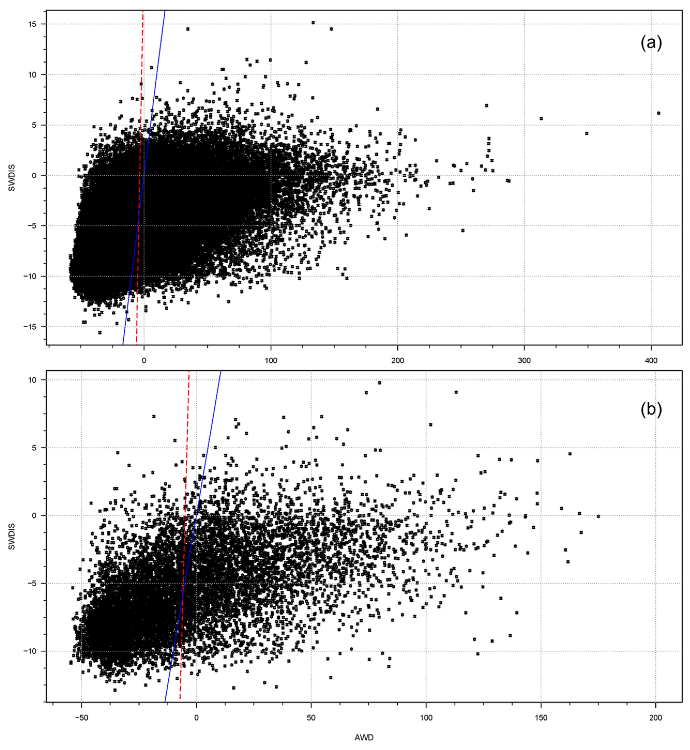
Figure 3.
Spatial distribution of Pearson’s correlation coefficients between the AWD and SWDIS from June 2010 to December 2013 for: (a) the entire year; and (b) the growing season. Whited cells depict gaps or omitted values.
Figure 3.
Spatial distribution of Pearson’s correlation coefficients between the AWD and SWDIS from June 2010 to December 2013 for: (a) the entire year; and (b) the growing season. Whited cells depict gaps or omitted values.

Figure 4.
As Figure 5, but for the Probability of Detection (POD) of drought weeks, (a) the entire year; and (b) the growing season.
Figure 4.
As Figure 5, but for the Probability of Detection (POD) of drought weeks, (a) the entire year; and (b) the growing season.
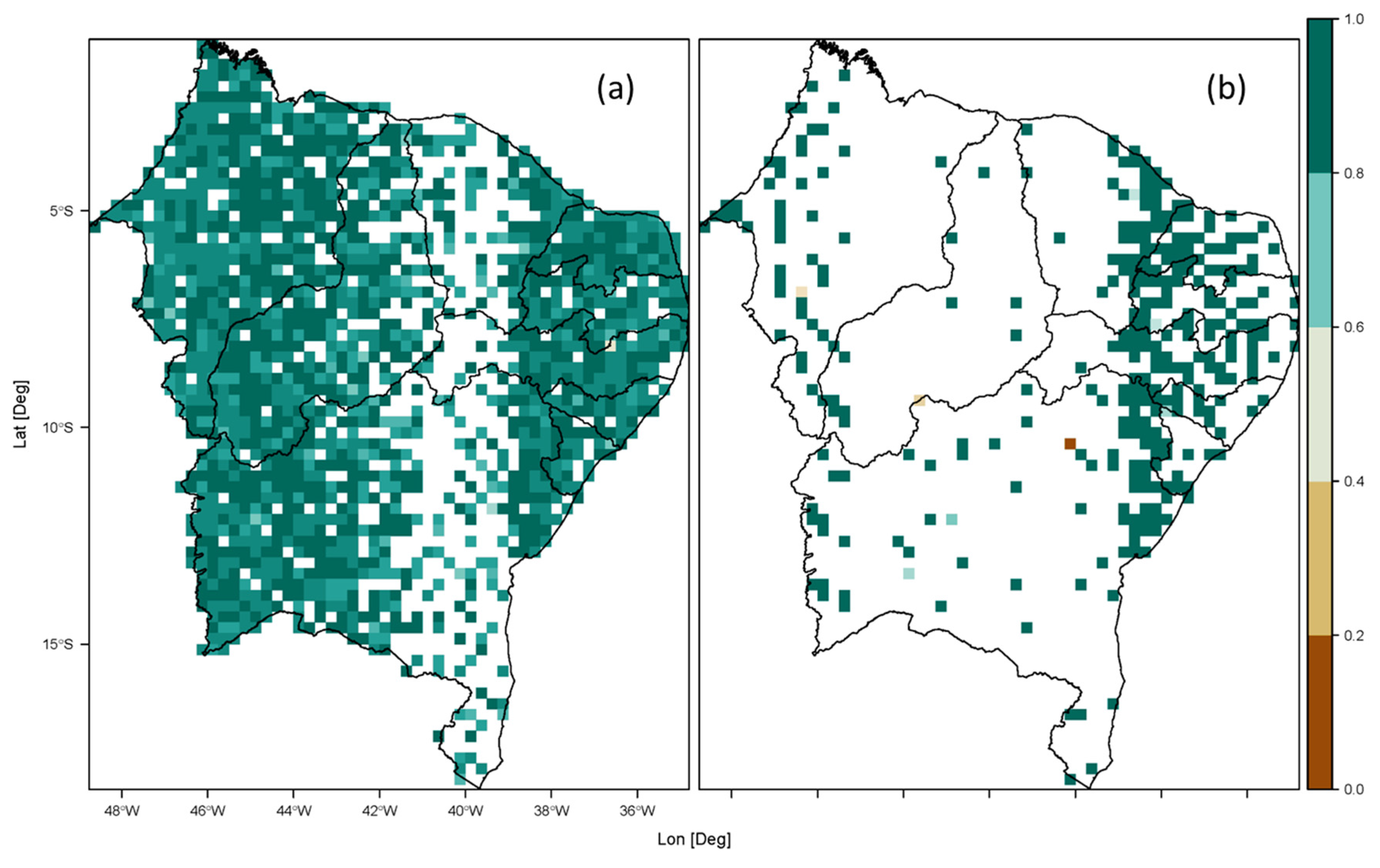
Figure 5.
Walter–Lieth climatic diagrams for the 1980–2013 period at: (a) Carnaubais (benchmark site # 1); (b) Campo Maior (benchmark site # 2); (c) Correntina (benchmark site # 3); (d) São Raimundo Nonato (benchmark site # 4); (e) Esperantinópolis (benchmark site # 5); and (f) Fazendas do Piauí (benchmark site # 6). Locations of benchmark sites are shown in Figure 1a. The black horizontal line indicates monthly precipitation greater than 100 mm and the graph over it is filled in solid blue. When P < 2T, where P is monthly mean precipitation, and T monthly mean temperature, there is a dry period (filled in dotted red vertical lines). Otherwise, the period is considered wet (filled in blue lines). Daily maximum average temperature of the hottest month and daily minimum average temperature of the coldest month are labeled in black at the left margin in each diagram.
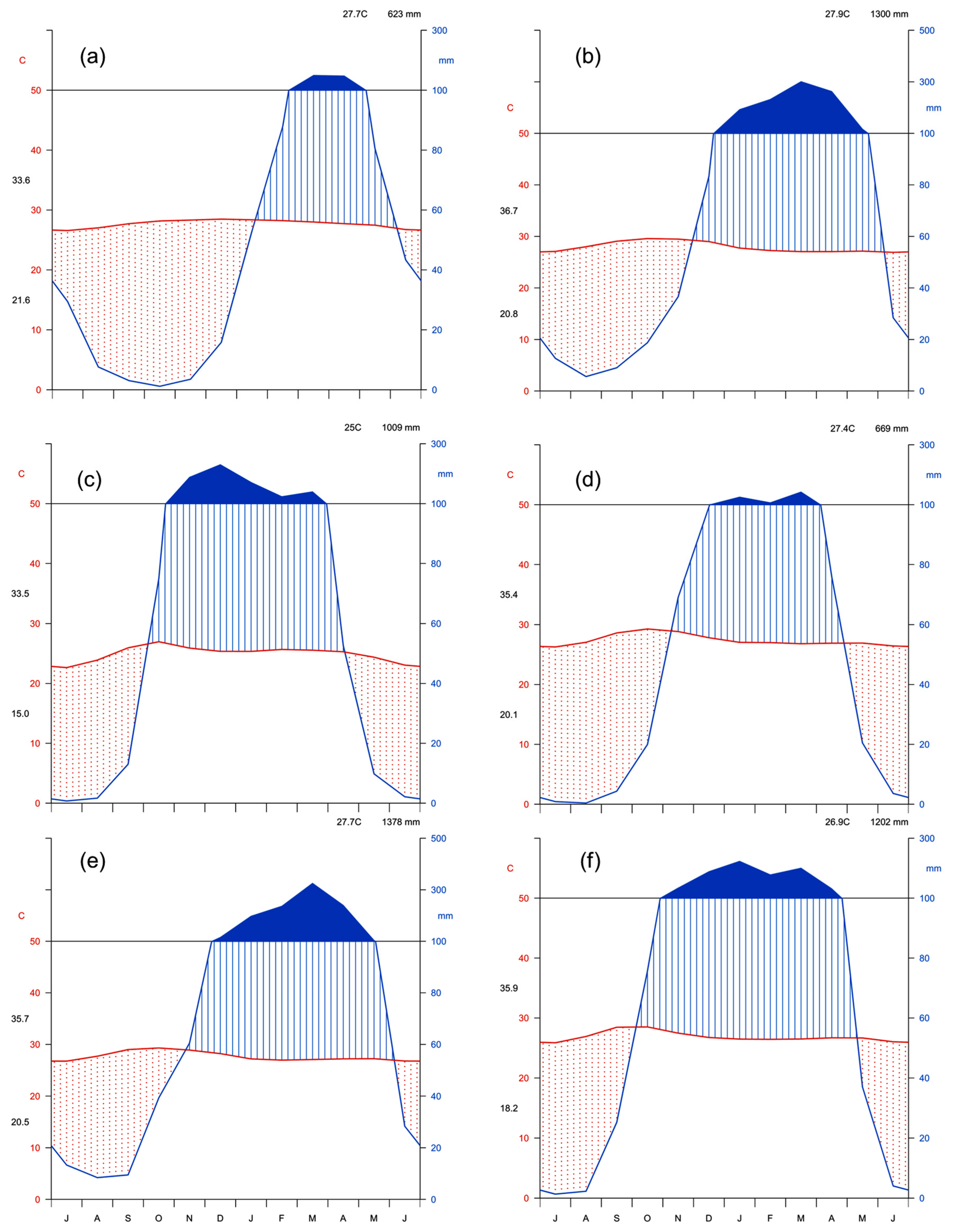
Figure 6.
Comparison of the temporal evolution of the AWD and SWDIS for the same benchmark sites displayed in Figure 5 from June 2010 to December 2013. The black and red lines depict the weekly values of AWD and SWDIS, respectively. The dashed vertical lines in each panel depict the end of 2010, 2011, 2012, and 2013, respectively. Whited segments indicate gaps or omitted values.

Figure 7.
Comparison of the Pearson’s linear coefficient between the SWDIS and AWD (r) against: (a) elevation (m.a.s.l.); (b) clay (%); (c) silt (%); (d) sand (%); (e) gaps (%); and (f) weekly average AWD (dimensionless) taking into account all benchmark sites. Numbers are the IDs shown in Table 1 and Table 2. Dashed red line depicts the linear regression best fit. Clay, silt, sand, and elevation were taken from Table 1, and gaps and r from Table 2.

Table 1.
Geographical and other information of benchmark sites.
| Id | Name/State | Biome 1 | Lat. (deg) | Lon. (deg) | Elevation 2 (m.a.s.l) | Soil Texture 3 (%) Clay-Silt-SAND | USDA Soil Taxonomy 3 | Soil Cover/Use |
|---|---|---|---|---|---|---|---|---|
| 1 | Carnaubais/RN | CAAT | −5.37 | −36.87 | 51 | 19-13-68 | Aquults | Cropland |
| 2 | Campo Maior/PI | CAAT | −4.87 | −42.12 | 128 | 22-23-56 | Aquults | Pasture |
| 3 | Correntina/BA | CER | −13.62 | −44.87 | 643 | 21-12-67 | Udox | Pasture |
| 4 | São Raimundo Nonato/PI | CAAT | −8.62 | −42.12 | 282 | 18-15-67 | Udults | Pasture |
| 5 | Esperantinópolis/MA | CER | −4.88 | −44.88 | 107 | 22-21-57 | Udults | Grassland |
| 6 | Fazendas do Piauí/PI | CER | −8.38 | −45.13 | 517 | 32-17-53 | Udults | Cropland |
Table 2.
Main statistical parameters for the SWDIS and AWD at benchmark sites.
| Id 1 | r 2 | Gaps (%) | SWDIS Mean | AWD Mean | SWDIS CV (%) | AWD CV (%) | P (mm/year) | T (°C) |
|---|---|---|---|---|---|---|---|---|
| 1 | 0.85 | 5.91 | −6.49 | −30.68 | 2.96 | 22.20 | 513 | 27.5 |
| 2 | 0.85 | 2.15 | −6.57 | −15.17 | 3.30 | 32.85 | 1102 | 28.5 |
| 3 | −0.10 | 14.52 | −5.20 | −10.78 | 3.15 | 38.89 | 1084 | 26.0 |
| 4 | 0.57 | 14.52 | −6.37 | −30.68 | 2.97 | 24.10 | 525 | 28.5 |
| 5 | 0.64 | 18.82 | −5.04 | −8.98 | 3.23 | 32.69 | 1303 | 29.0 |
| 6 | 0.02 | 13.98 | −5.34 | −11.65 | 2.82 | 29.56 | 1064 | 29.0 |
1 ID as in Table 1; 2 Pearson’s linear coefficient between the SWDIS and AWD. Gaps are referred to values of paired SWDIS-AWD; CV indicates the coefficient of variation in percentage. P and T depict the annual average precipitation and temperature during the period 2010–2013.
© 2017 by the authors. Licensee MDPI, Basel, Switzerland. This article is an open access article distributed under the terms and conditions of the Creative Commons Attribution (CC BY) license (http://creativecommons.org/licenses/by/4.0/).
Share and Cite
MDPI and ACS Style
Paredes-Trejo, F.; Barbosa, H. Evaluation of the SMOS-Derived Soil Water Deficit Index as Agricultural Drought Index in Northeast of Brazil. Water 2017, 9, 377. https://doi.org/10.3390/w9060377
AMA Style
Paredes-Trejo F, Barbosa H. Evaluation of the SMOS-Derived Soil Water Deficit Index as Agricultural Drought Index in Northeast of Brazil. Water. 2017; 9(6):377. https://doi.org/10.3390/w9060377
Chicago/Turabian StyleParedes-Trejo, Franklin, and Humberto Barbosa. 2017. "Evaluation of the SMOS-Derived Soil Water Deficit Index as Agricultural Drought Index in Northeast of Brazil" Water 9, no. 6: 377. https://doi.org/10.3390/w9060377
Note that from the first issue of 2016, this journal uses article numbers instead of page numbers. See further details here.