
A Stochastic Multi-Objective Chance-Constrained Programming Model for Water Supply Management in Xiaoqing River Watershed

MOE Key Laboratory of Regional Energy and Environmental Systems Optimization, College of Environmental Science and Engineering, North China Electric Power University, Beijing 102206, China
*
Author to whom correspondence should be addressed.
Water 2017, 9(6), 378; https://doi.org/10.3390/w9060378
Submission received: 23 March 2017
/
Revised: 24 May 2017
/
Accepted: 24 May 2017
/
Published: 27 May 2017
(This article belongs to the Special Issue Modeling of Water Systems)
Abstract
:In this paper, a stochastic multi-objective chance-constrained programming model (SMOCCP) was developed for tackling the water supply management problem. Two objectives were included in this model, which are the minimization of leakage loss amounts and total system cost, respectively. The traditional SCCP model required the random variables to be expressed in the normal distributions, although their statistical characteristics were suitably reflected by other forms. The SMOCCP model allows the random variables to be expressed in log-normal distributions, rather than general normal form. Possible solution deviation caused by irrational parameter assumption was avoided and the feasibility and accuracy of generated solutions were ensured. The water supply system in the Xiaoqing River watershed was used as a study case for demonstration. Under the context of various weight combinations and probabilistic levels, many types of solutions are obtained, which are expressed as a series of transferred amounts from water sources to treated plants, from treated plants to reservoirs, as well as from reservoirs to tributaries. It is concluded that the SMOCCP model could reflect the sketch of the studied region and generate desired water supply schemes under complex uncertainties. The successful application of the proposed model is expected to be a good example for water resource management in other watersheds.
1. Introduction
The watershed comprising social, economic and environmental factors has always played an important role in human survival and development. In recent decades, many watersheds around the world experienced serious water shortage crises under complex and interactive influences of natural and artificial factors, such as urbanization acceleration, socio-economic development, dramatic variation in hydrologic condition and frequent occurrence of extreme weather. As shown in incomplete statistical results, the annual average water consumption of China has exceeded 600 billion m3 and the annual average water deficit is 50 billion m3 [1]. Moreover, the average agricultural water utilization factor is 0.47, which is significantly lower than the global average level (0.7–0.8); the water consumption rate of ten thousand Yuan GDP is about 300 m3 and two times higher than the global average [2]. Therefore, effective utilization of limited water resources is an important task for local administrators. However, as a complex and huge system, a large amount of system factors and their intricate relationships lead to the fact that the watershed exhibits a variety of characteristics, such as integrality, dynamics, multidimensionality, nonlinearity and uncertainty. In order to realize sustainable water resource utilization, an appropriate water supply management model at a watershed scale is desired.
Previously, many uncertain analysis approaches were developed for dealing with watershed-scale water resource management issues, including stochastic mathematical programming (SMP) [3,4,5,6,7], fuzzy mathematical programming (FMP) [8,9,10,11] and interval mathematical programming (IMP) [12,13], as well as their combinations [14,15,16,17,18]. Among them, stochastic chance-constrained programming (SCCP) was extensively applied in water resource management due to its capacity in evaluating the trade-offs between realization of system objectives and satisfaction degrees of model constraints [19,20,21,22]. Nevertheless, the previous SCCP model also has a drawback in uncertainty expression and this may affect its applicability. In detail, the traditional SCCP model could normally handle the random variables with normal distributions. In fact, many parameters involved in practical water management systems may have other forms of probabilistic distributions, such as the log-normal type. As reported by Caldeira et al. [23], the observed statistical rainfall amounts are suitable to be expressed as log-normal distributions rather than normal ones. Moreover, the traditional SCCP method mostly aims to achieve a single economic objective, such as minimization of total system cost or maximization of total revenue. In practical applications, other objectives like the minimization of leakage loss or the groundwater utilization amounts may also need to be considered [24,25,26]. It is thus desired that an enhanced SCCP model with multiple objectives is being developed. Therefore, this study aims to propose a stochastic multi-objective chance-constrained programming model (SMOCCP) for handling the water supply issue on a watershed scale. This model consists of two objectives (i.e., the minimization of total system cost and the minimization of leakage loss) and is effective in dealing with random uncertainties expressed in log-normal distributions. The proposed model is capable of dealing with real-world complexity and generating reasonable allocation alternatives for water supply management. A water resources allocation problem in the Xiaoqing River watershed will be used to reflect the applicability of the proposed model. The rest of this paper will be organized as follows: the formulation and solution procedures of SMOCCP model are described in the “Methodology” section; the “Case Study” section describes the situation of the targeted watershed; the “Results Analysis” section will analyze the variation trend of generated solutions; the summary will be provided in the “Conclusion” section.
2. Methodology
2.1. Multi-Objective SCCP Model with Normal Probability Distribution
Referring to the previous studies [27,28,29], the general SCCP method could be used to solve SMP problems where both the left- and right-hand sides of uncertain variables in random constraints are expressed as random variables with normal probabilistic distributions. The multi-objective SMP model can be formulated as follows:
Subject to:
where f1 and f2 represent two objective functions; X is a vector of the decision variable; B(t) and D(t) are two sets with random factors defined on a probability space T, , which are described as B~N (mB, δB2) and D~N (mD, δD2), where mB and mD denotes the mean value, respectively; δB and δD denotes the standard deviation, respectively; A, C1 and C2 are fixed vectors of auxiliary variables. To solve model (1), the constraints (1c) and (1d) are converted into their deterministic equivalents through using the SCCP approach with a series of predefined constraints-violation levels qi. Meanwhile, two objective functions are combined into one objective through designing various weight coefficients (i.e., w1 and w2). The constraint (1e) ensures the non-negativity of decision vectors and nonzero of auxiliary variables. The model (1) is reformulated as follows:
Subject to:
where the term is the inverse form of the cumulative distribution function of the standard normally distributed random variable; the item is cumulative distribution function of Bi. The constraint (2d) regulated that the summation of two weight coefficients is equal to one. Finally, a variety of solutions (i.e., f1, opt, f2, opt and Xopt) are obtained through adjusting qi, w1 and w2 values, respectively.
2.2. Multi-Objective SCCP Model with Log-Normal Probability Distribution
As shown in the previous studies [30], some random variables in many real-world systems follow a log-normal probability distribution rather than a normal form. Referring to Model (2), a multi-objective SCCP model with log-normal random variables can be formulated as follows:
where B(t) and D(t) follow log-normal distribution forms, i.e., ln(B(t)) ~N (mB, δB2) and ln(D(t)) ~N (mD, δD2), respectively; variables B and D are expressed as and , respectively. The following four equations are established to reflect the interactive relationships among four feature parameters (i.e., mB, δB2, UB and VB2) [30].
Finally, different sets of solutions are obtained under various combinations of predefined qi levels and weight coefficients (w1 and w2). The commercial software LINGO (LINGO 12.0, Lindo System Inc., Chicago, IL, USA) is used to code and solve the SMOCCP model, because it is capable of providing the user-friendly edit interface, embedding a series of valuable equations and functions and solving the optimization model with unlimited variables and constraints. The short computation time of solving this model (just a few seconds) is convenient to generate a variety of solutions under specific combinations of weighted coefficients and constraints-violation levels. Figure 1 shows the procedures of formulating and solving the proposed SMOCCP model, which can be summarized as follows:
- Step 1:
- Gain in-depth insights into the targeted watershed system, identify all uncertain variables and design major system objectives and constraints;
- Step 2:
- Formulate a SMOCCP model;
- Step 3:
- Determine two solution algorithm rules associated with the multi-objective functions and the parameters presented as log-normal probability distributions;
- Step 4:
- Combine two objective functions into an integrated one and convert stochastic constraints to their respective crisp equivalents;
- Step 5:
- Obtain final solutions of f1, opt, f2, opt and Xopt under various probability levels and weight coefficients, respectively.
3. Case Study
3.1. Introduction and Problem Description of Xiaoqing River Watershed
The Xiaoqing River watershed (116°50′–118°45′ E and 36°15′–37°20′ N) is a major watershed in the Shandong province, where its area is almost 1033 km2 and reaches about 1/15 of total area in the Shandong Province. As shown in Figure 2, the main stream of the Xiaoqing River is sourced from four streamflows of the city Jinan with a total length of 237 km. It flows through ten regions (including towns and districts) of Jinan, Zibo, Binzhou, Dongying and Weifang from the west to the east, gathering the water from eighteen counties and finally falling into the bay Laizhou. As an important drainage channel, Xiaoqing River watershed is mainly responsible for agricultural irrigation and river transportation, and plays an important role in socio-economic development of the Shandong Province [31].
In recent decades, rapid socio-economic development of the cities around the watershed has made the Xiaoqing River the major water source and pollutant receiver. A number of problems were identified in this region’s water resource management [27]:
- (i)
- Severe water resource shortage and even flow cutoff in some tributaries: For example, the Jinan section of the Xiaoqing River is located in the mid-latitude zone in Northern China, where the rainfall distribution exhibits uneven characteristics and focuses on June to September, leading to frequent occurrences of drought and flooding disasters. The multi-year average surface runoff in this section is about 352.79 million m3, which is far below the required water demands.
- (ii)
- Poor water quality: the Xiaoqing River receives industrial, agricultural and household wastewater sourced from eighteen counties, resulting in significant degradation of water quality. As stated in the “Report on the Water Quality of Critical Water Function Areas in the Shandong Province”, the total length of evaluated river is roughly 1682.6 km. Among them, the river length for meeting the water quality requirement is only 590.2 km, while the polluted river length reaches 1092 km.
- (iii)
- Imperfect infrastructure and management regime of this watershed: The overly high leakage loss of the water-transportation pipeline leads to a reduced amount of available water resources. A separate management mechanism is applied to this watershed for the time being, leading to unclear definitions in rights, responsibilities and obligations for the watershed management.
Therefore, the way through the optimal allocation and scientific scheduling of water resources is critical for meeting users’ demand, controlling pollutants and achieving sustainable socio-economic development.
3.2. Generalization of Xiaoqing River Watershed
According to natural conditions, geographical position, surface runoff and drainage characteristics of the Xiaoqing River watershed and the distribution of its water projects, the water supply management system for this watershed is conceptualized as 20 nodes, including two water sources, four disposal facilities, seven reservoirs and seven users. Moreover, the interconnected tributaries and water diversion channels are described as the lines between the nodes. Finally, the system network technique is used to establish the configuration network diagram for this watershed (see Figure 3), which includes multiple water sources (surface water and groundwater), multiple projects (water storage, treatment and transportation projects), multiple water transmission systems (surface water transmission and groundwater replenishment system) and multiple user systems (industrial, agricultural and domestic users). Within this watershed management system, two water sources are defined, including surface water and groundwater. It is regulated that the water drawn from surface sources should be purified by the treatment facilities, i.e., First Water Purification Plant, Second Water Purification Plant, Dajin Sewage Treatment Plant and Tantou Sewage Treatment Plant, respectively. Next, the purified surface water and groundwater are transferred to the reservoirs, including Dazhan Reservoir, Duzhuang Reservoir, Mengshan Reservoir, Duozhuang Reservoir, Xinglin Reservoir, Langmaoshan Reservoir and Taihe Reservoi. Finally, the water in the reservoirs are supplied to seven tributaries for industrial, agricultural and domestic utilizations along the rivers, which are Lashan River, Daxinshi River, Hancang River, Xiujiang River, Luo River, Liugong River and Yangjia River. The water allocation and provision schemes among various nodes are determined by solving the optimization model.
3.3. System Parameters and Model Formulation
The system parameters are mainly used to describe the nodes’ characteristics and the connections among them. Table 1 describes inventory amounts of water sources and inventory amounts and storage capacities of the treatment facilities and reservoirs. Table 2 lists the costs and leakage rate of water transportation paths. Particularly, the water demand in tributaries is influenced by many factors, including required water demands from industry, agriculture and residents along the river, natural supplies (precipitation) and the lowest environmental flow demands. As shown in a statistical analysis of historical data, it is assumed that the required water amounts are expressed in stochastic forms with log-normal distributions (shown in Table 3). Based on the theoretical Model (3), a multi-objective water supply management model for the Xiaoqing River watershed can be formulated as follows [12,30]:
Objective function:
where f1 = total system cost (RMB); k (k = 1, 2, …, K) = the index of time periods (i.e., months) where K is total number of time period; j (j = 1, 2, ..., J) = the index of water sources, where J is total number of water sources; t (t = 1, 2, …, T) = the index of treatment plants, where T = the total number of treatment plants; r (r = 1, 2, …, R) = the index of reservoirs, where R is total number of reservoirs; z (z = 1, 2, …, Z) is the index of tributaries, where Z is total number of tributaries; XJTjtk = the decision variables denoting water amounts transferred from water source to treatment plant, (×103 m3); XTRtrk = the decision variables denoting water amounts allocated from treatment plant to reservoir, (×103 m3); XRZrzk = the decision variables representing water amounts transferred from reservoir to tributary, (×103 m3); PRjk = water purchase cost from water source per month (RMB/ × 103 m3); CJTjt = water transfer cost from source to treatment plant (RMB/ ×103 m3); CTRtr = water transfer cost from treatment plant to reservoir (RMB/ × 103 m3); CRZtr = water transfer cost from reservoir to tributary (RMB/ × 103 m3); f2 = total leakage loss (×103 m3); LXJjt = leakage loss in network from source to treatment plant, (%); LXTtr = leakage loss in network from treatment plant to reservoir, (%); LXZrz = leakage loss in network from reservoir to tributary, (%). The objective Function (5a) is to minimize total system costs, which is calculated through the summation of water purchase and transportation costs. The decision variables are transferred water amounts among water sources, treatment plants, reservoirs and tributaries, respectively. The objective Function (5b) aims to achieve the minimization of total leakage loss in the entire transportation process.
Subject to:
- (1)
- Water consumption constraints:where Dzk(ω) = required water amounts of tributary in each month (×103 m3), which follows the log-normal distribution, i.e., ln(Dzk(ω)) ~N (mD, δD2); ZRZrz = binary variable (0 or 1) used to define paths from reservoir to tributary; URZ = the maximum capacity of prescribed paths from reservoir to tributary (×103 m3). The constraint (5c) is used to regulate allocated water amounts to tributaries that are higher than their required amounts. The constraint (5d) is used to ensure that water is transferred in prescribed paths where the paths are available while binary variable ZRZrz is “1”; otherwise, it will be “0”.
- (2)
- Reservoir constraints:where IROr = inventory amounts of reservoir at the first planning phase, (×103 m3); IRrk = inventory amounts of reservoir at the end of month, (×103 m3); ZTRtr = binary variables (0 or 1) used to regulate the paths from treatment plant to reservoir; UTR = the maximum capacities of prescribed paths from treatment plant to reservoir, (×103 m3); VRrk = reservoir’s capacities at month, (×103 m3). The constraints (5e) and (5f) reflected the water connections among treatment plants, reservoirs and tributaries, respectively. The constraint (5g) is used to ensure that the water is transferred in prescribed paths. The constraint (5h) regulated that water amounts provided by the reservoirs should be lower than the maximum capacities of reservoirs.
- (3)
- Treatment plant constraints:where ITOt = inventory amounts of treatment plants at the first planning phase, (×103 m3); ITtk = inventory amounts of treatment plants at the end of month, (×103 m3); ZJTjt = binary variable (0 or 1) used to define paths from source to treatment plant; Ujt = the maximum capacity of prescribed paths from water source to treatment plant, (×103 m3); VTtk = treatment capacities at month, (×103 m3). The constraints (5i) and (5j) are used to reflect the hydraulic relation among water sources, treatment plants and reservoirs, respectively. The constraint (5k) regulated the water must be allocated in the prescribed paths. The constraint (5l) regulated that treated water amounts by the plants should be lower than the maximum capacities of treatment plants.
- (4)
- Water source constraints:where IJOj = inventory amounts of each water source at the first phase (×103 m3); IJjk = inventory amounts at the end of month (×103 m3); BJjk = recovered water amount from water source, (×103 m3); MJjk = the maximum water amount extracted from water source at month, (×103 m3). The constraints (5m) and (5n) are used to reflect the relationship among water sources and treatment plants, respectively. The constraint (5o) is used to ensure that the water extracted from water sources should be lower than their maximum capacities.
- (5)
- Technical constraintswhere the constraint (5p) is used to ensure all decision variables are positive. Referring to the model (3), the constraint (5b) is converted into its deterministic equivalent, such that the model (5) would become a general deterministic optimization model, and optimal solutions (i.e., f1,opt, f2,opt, XJTjtk, XTRtrk and XRZrzk) are obtained under various weight combinations and constraint-violation levels.
4. Result Analysis and Discussion
4.1. Result Analysis
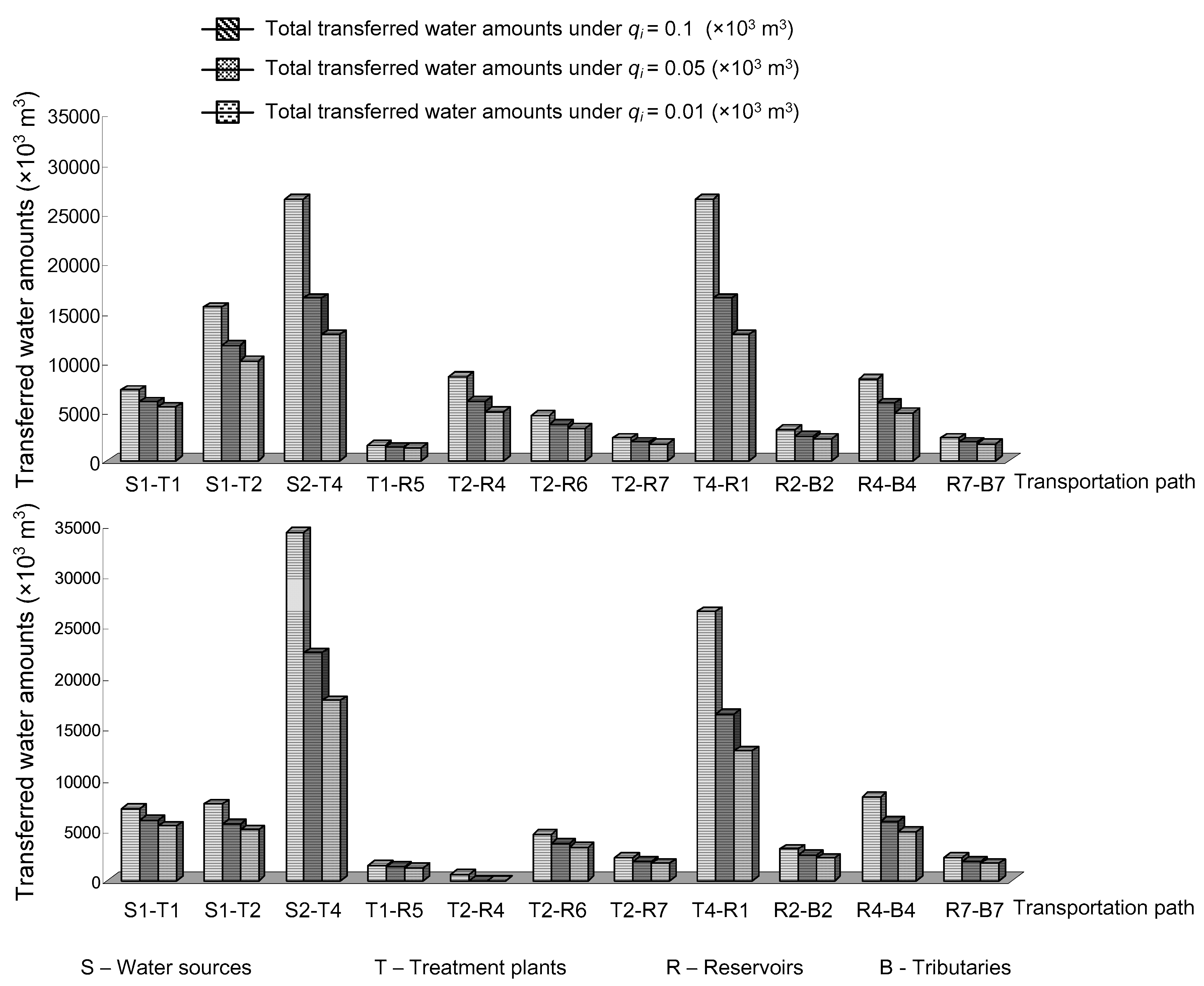
In order to reflect the interactive effects of designed weight combinations and constraint violation levels on generated solutions, a large amount of literature reviews and model tests are conducted. Firstly, referring to the previous studies [29,32], three violation levels are considered, i.e., 0.01, 0.05 and 0.1. Secondly, after a series of tests for various combinations of weight coefficients, two groups of extreme weight coefficient values are determined, i.e., (i) 0.9 and 0.1, and (ii) 0.1 and 0.9. As shown in Table 4, the change in designed violation levels and weight values leads to notable variation of results (i.e., decision variables and objective function). Table 4 provides part of the solutions from the SMOCCP model, in terms of transferred water amounts among water sources, treatment plants, reservoirs and tributaries in each month, respectively. In order to better reflect the influences exerted by designed weight coefficients and violation levels on obtained solutions, the total transferred water amounts over all planning periods are calculated and their variation trends are shown in Figure 4.
Considering the obtained solutions are affected by an interactive effect of the above two factors, the variation trend of the solutions is analyzed under the context of changing one factor at a time. Firstly, when two weight coefficients stay stable (w1 = 0.9 and w2 = 0.1) and the probabilistic level (i.e., qi) increases over twelve months, the total water amounts supplied to seven tributaries would decrease. For example, as shown in Table 4, at qi levels of 0.01, 0.05 and 0.1, the water amounts transferred to tributary 2 in the first period are 240.15, 197.44 and 177.88 × 10³ m3, respectively; similarly, the water amounts allocated to tributary 7 in the second period are 156.46, 135.88 and 126.05 × 10³ m3, respectively. The reason behind such a difference is that the water demand constraint is involved in the stochastic variables, where the required water amounts of the tributaries were expressed as random variables with log-normal distributions. Therefore, the increase in violation level of qi means that the satisfaction level of the constraint would decrease, leading to a decrease of the water demand. The intrinsic balanced relationship between water supply and demand determined that a decrease in water demand must be accompanied with a decrease in the water amounts extracted from water sources. As shown in Figure 4, as the probability level increases, the total water amounts extracted from the groundwater would decrease (i.e., 26,418.10, 16,381.95 and 12,724.73 × 103 m3, respectively); similarly, the water amounts provided by surface water would be 22,587.89, 17,600.33 and 15,454.30 × 103 m3, respectively. In fact, the decrease in required water amounts leads to the decrease in transferred water amounts in the entire water management system, such that the total leakage loss and total system costs (including supplied, treated and transferred costs) would decrease. At three qi values (i.e., 0.01, 0.05 and 0.1), the total leakage loss amounts are 19,055.62, 12,813.74 and 10,440.01 × 103 m3, respectively. Correspondingly, the total system costs are 51.56, 34.48 and 28.02 × 10⁶ RMB, respectively.
The same variation trend also appears under another weight combination, where two weight coefficients w1 and w2 are equal to 0.1 and 0.9, respectively. As the qi value increases from 0.01 to 0.1, the water amounts allocated to tributary 4 in the third period would be 631.59, 451.01 and 376.90 × 10³ m3, respectively (see Table 5). As shown in Figure 4, the water amounts drawn from the surface water are 14,658.54, 11,545.56 and 10,428.10 × 103 m3, respectively; the water amounts sourced from groundwater are 34,268.16, 22,376.18 and 17,700.67 × 103 m3, respectively. The total leakage loss rates are 18,976.33, 12,753.19 and 10,389.75 × 103 m3, respectively, and the total system costs are 54.01, 36.34 and 29.57 × 10⁶ RMB, respectively. The above variations in the objective functions and decision variables reflect the trade-off between system objective realization and constraint satisfaction degree. A low water requirement is associated with a reduced amount of water supply, a low leakage loss and a low system cost, which means an improvement in system efficiency. Nevertheless, the system-failure risk would become high due to insufficient water provision. Conversely, a higher system cost could ensure that the water demand is better satisfied and the system remains more stable.
The variation situations of the obtained solutions under fixed probabilistic levels are also discussed in order to examine the influences caused by weight design on generated decision schemes. Firstly, the selection of water sources exhibits an obvious influence under various weight combinations. For example, the surface water is the favorite option where the system cost is more seriously concerned (where w1 = 0.9 and w2 = 0.1). Under qi values of 0.01, 0.05 and 0.1, the difference values between extracted surface water amounts and groundwater amounts are −3830.21, 1218.38 and 2729.57 × 103 m3, respectively. Conversely, when the leakage loss is considered as a critical factor, the groundwater becomes a preferred source, where the difference values are −19,609.62, −10,830.62 and −7272.57 × 103 m3, respectively. This is because the leakage loss situation occurs in the transportation path between surface water and treatment plants. Moreover, the selection of the transportation path is also dependent on the weight coefficients. For example, it is required that the tributary 7 is able to receive the water drawn from treatment plants 2 and 4, respectively. The path between treatment plant 2 and tributary 7 is adopted due to its low leakage loss. At three probabilistic levels, the transferred water amounts are 2281.57, 1890.30 and 1711.34 × 103 m3, respectively. A similar situation is also reflected in tributary 5, which receives the water sourced from treatment plant 1, rather than plant 2. The received water amounts are 1533.50, 1361.36 and 1277.75 × 103 m3, respectively. The variations in the weight coefficients not only affect the decision variables, but also the objective values. Under the economic-prior condition (w1 = 0.9 and w2 = 0.1), the low costs are expected (namely 51.56, 34.48 and 28.02 ×10⁶ RMB, respectively). Meanwhile, the high leakage losses are unavoidable (i.e., 19,055.62, 12,813.74 and 10,440.01 × 103 m3, respectively). Conversely, when the resource protection obtains more attention (w1 = 0.1 and w2 = 0.9), the low leakage loss amounts and the high operational costs would be expected (i.e., the two groups of objective values are 18,976.33, 12,753.19 and 10,389.75 × 103 m3 and 54.01, 36.34 and 29.57 × 10⁶ RMB, respectively).
In real-world applications, how to choose an appropriate solution as a decision basis mainly depends on local situations. As shown in statistical analysis of historical data, the water storage situation in the targeted watershed has worsened over recent years. Moreover, the water-shortage crisis is exacerbated, since available water amounts mainly rely on seasonal rainfall, leading to unstable water provision. The frequent occurrence of extreme events (i.e., dry or flood) due to global climate change is also affecting water resource protection and utilization. Under such a background, the design and generation of a water provision strategy should meet the user’s requirement as much as possible. Therefore, in this study, the decision alternative under probabilistic level of 0.99 at the condition of w1 = 0.1 and w2 = 0.9 is recommended as the decision basis for decision-making due to their robust characteristics, although the high system costs are inevitable. The successful application of the SMOCCP model in the Xiaoqing River watershed provides a good example for other watersheds in solving similar problems.
Generally, the study results demonstrated that the SMOCCP model owns advantages in terms of methodological development and practical applicability, which is effective in tackling the water supply management problem under complexities and uncertainties. In detail, from the methodological aspect, the log-normal based SCCP model, as an improved version of the traditional SCCP model, is effective in describing the random variables as log-normal distribution, rather than normal distribution. It overcomes the main limitation of the traditional SCCP model, which is incapable of handling the random variables presented as non-normal forms. In terms of practical applications, the results of required water amounts showed a log-normal distribution. As a critical variable of the water supply management system, the accurate expression of water demand is beneficial for generating rational water allocation schemes.
4.2. Discussion
In this section, a sensitivity analysis is conducted for reflecting the sensitive extent of the proposed SMOCCP model to its critical parameters. The cost coefficients and leakage loss rates are considered as the major sensitive parameters, where the variation range of cost coefficients is divided into seven levels including −25%, −50%, −75%, 1, +25%, +50%, and 75%. Correspondingly, the range of leakage rate is assumed as −0.99%, −0.66%, −0.33%, 1, 0.33%, 0.66% and 0.99%. The influences caused by the parameter variations on generated objective function values are shown in Table 6 and Table 7. It is found that the changes in the cost coefficients only lead to the variation in the total system costs, where the change ranges of cost coefficients and system costs are the same. Conversely, the varied leakage rates would cause the change in total system costs and leakage loss rates simultaneously. Therefore, more attention should be paid to the investigation and evaluation process of leakage loss rates in order to ensure the accuracy and reliability of the generated decision scheme.
Moreover, the SMOCCP model still needs to be improved, especially in the following three aspects. Firstly, the hydrological processes and hydraulic connections in the water provision network are described by some simplified mathematical equations. This provides the conveniences in establishing the water allocation optimization model, but may neglect some essential factors and critical processes and compromise somewhat the accuracy of generated solutions. Therefore, how to incorporate some simulated results of mature hydrological models into the proposed optimization model deserves further research. Secondly, as the major goal of this research is to demonstrate the SCCP model with log-normal distribution, the simple weight summation approach is used to solve the SMOCCP model. In fact, many types of multi-objective methods are available, such as the ε-constraint method, minimax approach and genetic algorithm. Among them, the genetic algorithm is capable of realizing the convergence to the Pareto-optimal front and is applied in many fields extensively [33,34,35]. Therefore, it definitely has a potential to solve this model and the related topics deserve further investigations. Thirdly, the SMOCCP model belongs to the type of the SMP model. Two other types of uncertain optimization techniques, i.e., FMP and ILP, could be incorporated for handling more complex management problems.
5. Conclusions
In this study, a stochastic multi-objective chance-constrained programming model (SMOCCP) was developed. It allows random variables to be expressed in log-normal distributions instead of normal ones. As shown in the statistical results, the required water amounts exhibited log-normal distribution characteristics. Therefore, a SMOCCP model was established to solve the water supply management problem in the Xiaoqing River watershed. The generation of rational and effective water supply strategies showed that the SMOCCP model could reflect the complexity of the studied watershed and obtain desired water supply schemes under uncertainties. In order to enhance the applicability and feasibility of the SMOCCP model, further studies on how to incorporate some simulation results of hydrological models into the SMOCCP model and how to utilize other types of multi-objective solution algorithms are expected. Meanwhile, other uncertain analysis techniques, including ILP and SMP, have potentials to be further integrated into a SMOCCP model.
Acknowledgments
This research was supported by the National Basic Research Program of China (2013CB430406) and the Fundamental Research Funds for the Central Universities. The authors deeply appreciate the anonymous reviewers for their insightful comments and suggestions which contributed much to improving the manuscript.
Author Contributions
Ye Xu designed the research with co-authors, analyzed the data; formulated the optimization model, and wrote the paper with the co-authors. Wei Li and Xiaowen Ding gave the comments and helped to revise the paper.
Conflicts of Interest
The authors declare no conflict of interest.
References
- Cai, J.L.; Varis, L.; Yin, H. China’s water resources vulnerability: A spatio-temporal analysis during 2003–2013. J. Clean. Prod. 2017, 142, 2901–2910. [Google Scholar] [CrossRef]
- Cao, X.C.; Wang, Y.B.; Wu, P.; Zhao, X.N.; Wang, J. An evaluation of the water utilization and grain production of irrigated and rain-fed croplands in China. Sci. Total Environ. 2015, 529, 10–20. [Google Scholar] [CrossRef] [PubMed]
- Huang, G.H.; Loucks, D.P. An inexact two-stage stochastic programming model for water resources management under uncertainty. Civ. Eng. Environ. Syst. 2000, 17, 95–118. [Google Scholar] [CrossRef]
- Haguma, D.; Leconte, R.; Krau, S.; Cote, P.; Brissette, F. Water Resources Optimization Method in the Context of Climate Change. J. Water Resour. Plan. Manag. 2015, 141, 04014051. [Google Scholar] [CrossRef]
- Tan, Q.; Huang, G.H.; Cai, Y.P.; Yang, Z.F. A non-probabilistic programming approach enabling risk-aversion analysis for supporting sustainable watershed development. J. Clean. Prod. 2016, 112, 4771–4788. [Google Scholar] [CrossRef]
- Rouge, C.; Tilmant, A. Using stochastic dual dynamic programming in problems with multiple near-optimal solutions. Water Resour. Res. 2016, 52, 4151–4163. [Google Scholar] [CrossRef]
- Davidsen, C.; Pereira-Cardenal, S.J.; Liu, S.X.; Mo, X.G.; Rosbjerg, D.; Bauer-Gottwein, P. Shortage management modeling for urban water supply systems. J. Water Resour. Plan. Manag. 2015, 141, 04014086. [Google Scholar] [CrossRef]
- Maeda, S.; Kuroda, H.; Yoshida, K.; Tanaka, K. A GIS-aided two-phase grey fuzzy optimization model for nonpoint source pollution control in a small watershed. Paddy Water Environ. 2017, 15, 263–276. [Google Scholar] [CrossRef]
- Xu, T.Y.; Qin, X.S. Solving water management problem through combined genetic algorithm and fuzzy simulation. J. Environ. Inf. 2013, 22, 39–48. [Google Scholar] [CrossRef]
- Xu, T.Y.; Qin, X.S. Integrating decision analysis with fuzzy programming: Application in urban water distribution system operation. J. Water Resour. Plan. Manag. 2014, 140, 638–648. [Google Scholar] [CrossRef]
- Xu, T.Y.; Qin, X.S. A sequential fuzzy model with general-shaped parameters for water supply-demand analysis. Water Resour. Manag. 2015, 29, 1431–1446. [Google Scholar] [CrossRef]
- Qin, X.S.; Xu, Y. Analyzing urban water supply through an acceptability-index-based interval approach. Adv. Water Resour. 2011, 34, 873–886. [Google Scholar] [CrossRef]
- Zhou, F.; Dong, Y.J.; Wu, J.; Zheng, J.L.; Zhao, Y. An Indirect Simulation-Optimization Model for Determining Optimal TMDL Allocation under Uncertainty. Water 2015, 7, 6634–6650. [Google Scholar] [CrossRef]
- Cai, Y.P.; Huang, G.H.; Wang, X.; Li, G.C.; Tan, Q. An inexact programming approach for supporting ecologically sustainable water supply with the consideration of uncertain water demand by ecosystems. Stoch. Environ. Res. Risk A 2011, 25, 721–735. [Google Scholar] [CrossRef]
- Dai, C.; Cai, Y.P.; Liu, Y.; Wang, W.J.; Guo, H.C. A generalized interval fuzzy chance-constrained programming method for domestic wastewater management under uncertainty—A case study of Kunming, China. Water Resour. Manag. 2015, 29, 3015–3036. [Google Scholar] [CrossRef]
- Dong, C.; Tan, Q.; Huang, G.H.; Cai, Y.P. A dual-inexact fuzzy stochastic model for water resources management and non-point source pollution mitigation under multiple uncertainties. Hydrol. Earth Syst. Sci. 2014, 18, 1793–1803. [Google Scholar] [CrossRef]
- Fan, Y.R.; Huang, G.H.; Guo, P.; Yang, A.L. Inexact two-stage stochastic partial programming: Application to water resources management under uncertainty. Stoch. Environ. Res. Risk A 2012, 26, 281–293. [Google Scholar] [CrossRef]
- Fan, Y.R.; Huang, G.H.; Huang, K.; Baetz, B.W. Planning water resources allocation under multiple uncertainties through a generalized fuzzy two-stage stochastic programming method. IEEE Trans. Fuzzy Syst. 2015, 23, 1488–1504. [Google Scholar] [CrossRef]
- Guo, P.; Huang, G.H. Two-stage fuzzy chance-constrained programming: Application to water resources management under dual uncertainties. Stoch. Environ. Res. Risk A 2009, 3, 349–359. [Google Scholar] [CrossRef]
- Sreekanth, J.; Datta, B.; Mohapatra, P.K. Optimal short-term reservoir operation with integrated long-term goals. Water Resour. Manag. 2012, 10, 2833–2850. [Google Scholar] [CrossRef]
- Jothiprakash, V.; Arunkumar, R.; Rajan, A.A. Optimal crop planning using a chance constrained linear programming model. Water Policy 2011, 5, 734–749. [Google Scholar] [CrossRef]
- Guo, P.; Wang, X.L.; Zhu, H.; Li, M. Inexact fuzzy chance-constrained nonlinear programming approach for crop water allocation under precipitation variation and sustainable development. J. Water Resour. Plan. Manag. 2014, 9, 05014003. [Google Scholar] [CrossRef]
- Caldeira, T.L.; Beskow, S.; de Mello, C.R.; Faria, L.C.; de Souza, M.R.; Guedes, H.A.S. Probabilistic modelling of extreme rainfall events in the Rio Grande do Sul state. Rev. Bras. Eng. Agric. Ambient. 2015, 19, 197–203. [Google Scholar] [CrossRef]
- Fattahi, P.; Fayyaz, S. A compromise programming model to integrated urban water management. Water Resour. Manag. 2010, 24, 1211–1227. [Google Scholar] [CrossRef]
- Han, Y.; Xu, S.G.; Xu, X.Z. Modeling multisource multiuser water resources allocation. Water Resour. Manag. 2008, 22, 911–923. [Google Scholar] [CrossRef]
- Yang, W. A multi-objective optimization approach to allocate environmental flows to the artificially restored wetlands of China’s Yellow River Delta. Ecol. Model. 2011, 222, 261–267. [Google Scholar] [CrossRef]
- Huang, G.H. A hybrid inexact-stochastic water management model. Eur. J. Oper. Res. 1996, 107, 137–158. [Google Scholar] [CrossRef]
- Kursad, A.; Hadi, G. A chance-constrained approach to stochastic line balancing problem. Eur. J. Oper. Res. 2007, 180, 1098–1115. [Google Scholar]
- Xu, Y.; Huang, G.H.; Qin, X.S.; Cao, M.F. SRCCP: A stochastic robust chance-constrained programming model for municipal solid waste management under uncertainty. Resour. Conserv. Recycl. 2009, 53, 352–363. [Google Scholar] [CrossRef]
- Daniel, M.Z.; Kramer, R.A.; Taylor, B.; Sarin, S.C. Chance constrained programming models for risk-based economic and policy analysis of soil conservation. Agric. Resour. Econ. Rev. 1994, 23, 58–65. [Google Scholar]
- Cui, B.S.; Wang, C.F.; Tao, W.D.; You, Z.Y. River channel network design for drought and flood control: A case study of Xiaoqinghe River basin, Jinan City, China. J. Environ. Manag. 2009, 90, 3675–3686. [Google Scholar] [CrossRef] [PubMed]
- Xu, Y.; Huang, G.H.; Xu, T.Y. Inexact Management Modeling for Urban Water Supply Systems. J. Environ. Inf. 2012, 20, 34–43. [Google Scholar] [CrossRef]
- Xu, G.; Yang, Y.Q.; Liu, B.B.; Xu, Y.H.; Wu, A.J. An efficient hybrid multi-objective particle swarm optimization with a multi-objective dichotomy line search. J. Comput. Appl. Math. 2015, 280, 310–326. [Google Scholar] [CrossRef]
- Ahmadi, A.; Tiruta-Barna, L. Process modelling-life cycle assessment-multiobjective optimization tool for the eco-design of conventional treatment processes of potable water. J. Clean. Prod. 2015, 100, 116–125. [Google Scholar] [CrossRef]
- Vazhayil, J.P.; Balasubramanian, R. Optimization of India’s electricity generation portfolio using intelligent Pareto-search genetic algorithm. Int. J. Electr. Power 2014, 55, 13–20. [Google Scholar] [CrossRef]
Figure 1.
Formulation and solution framework of the stochastic multi-objective chance-constrained programming model (SMOCCP) model.
Figure 1.
Formulation and solution framework of the stochastic multi-objective chance-constrained programming model (SMOCCP) model.
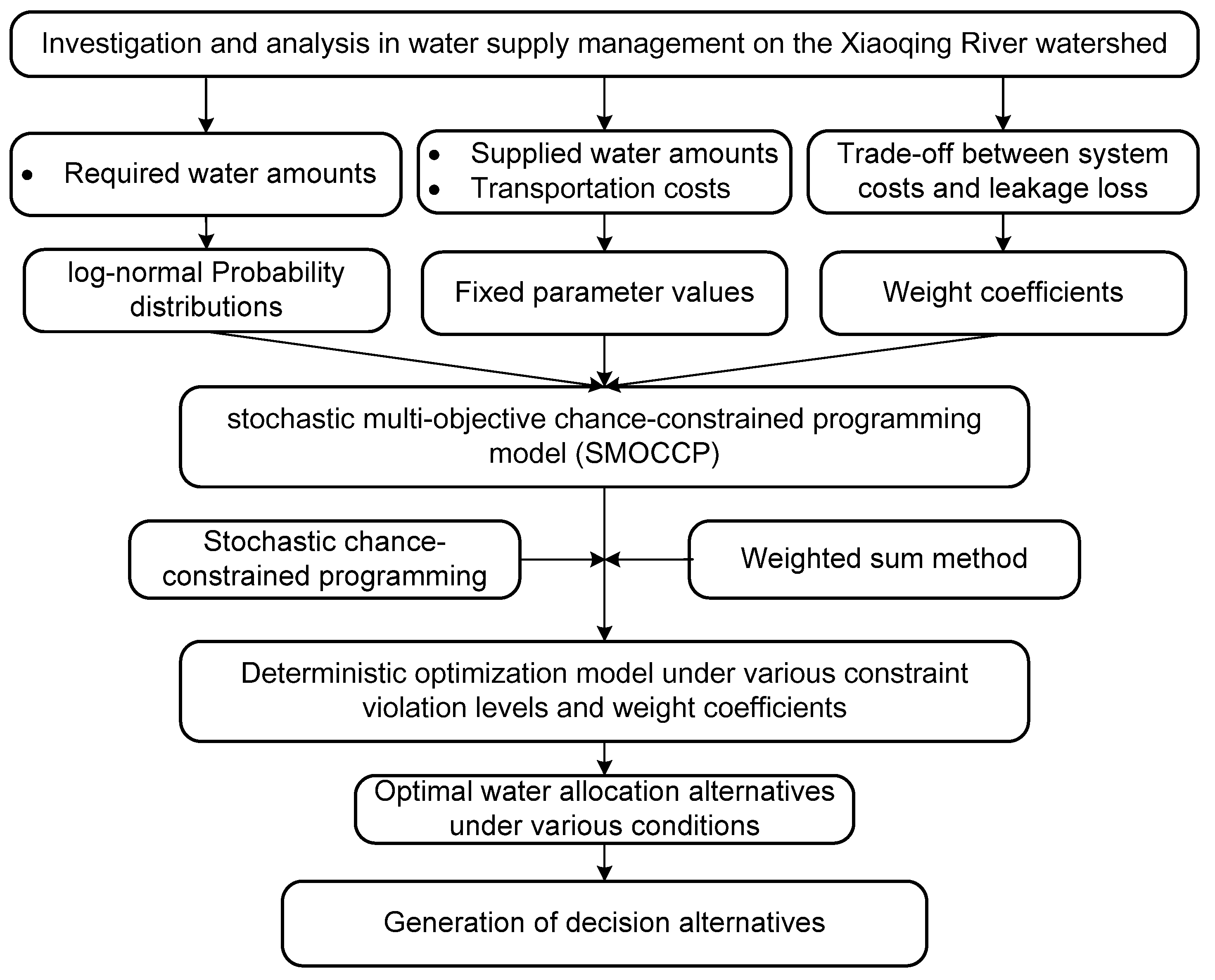
Figure 2.
The demonstration of the Xiaoqing River watershed.
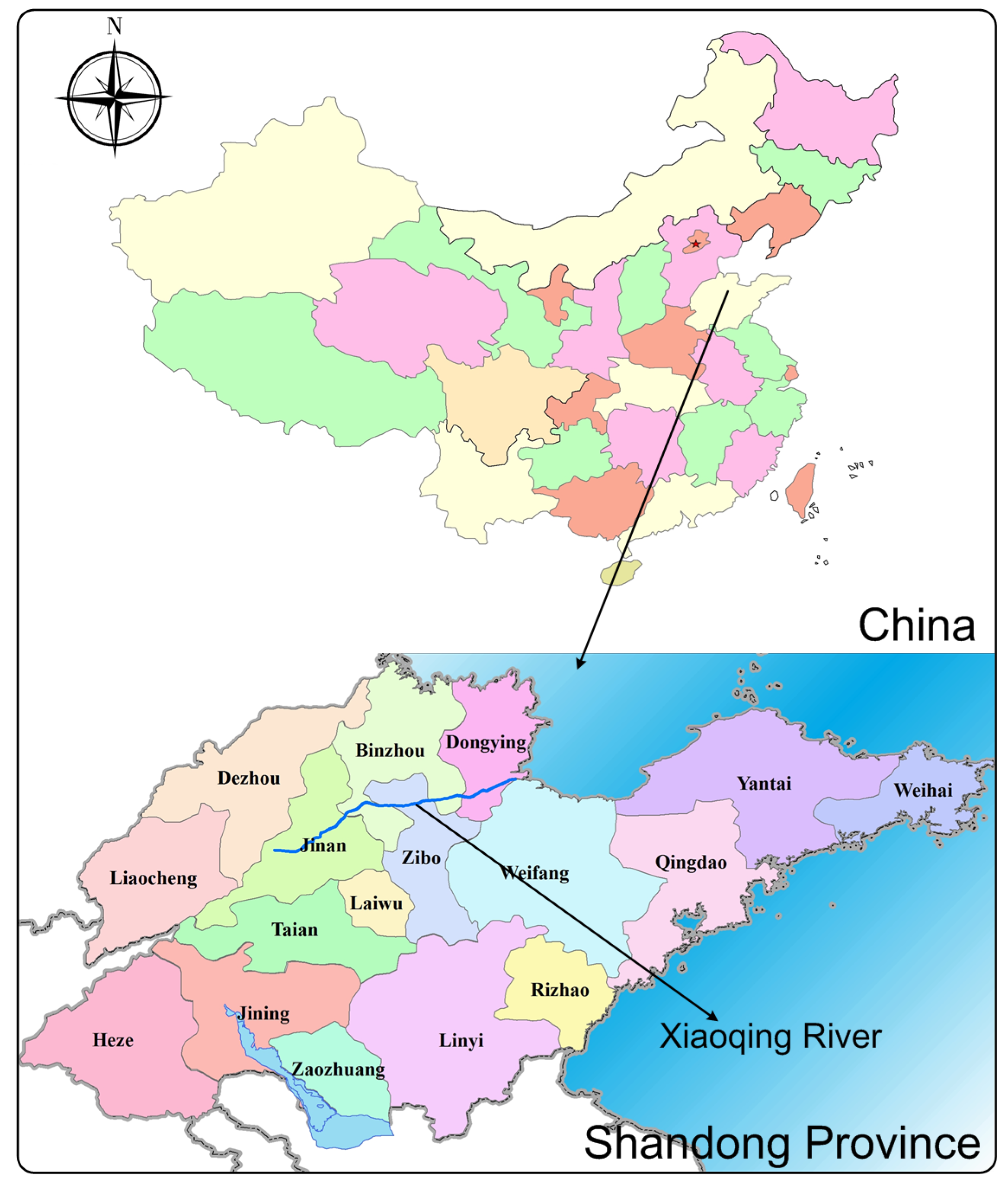
Figure 3.
Flow diagram of the water supply management system in the watershed.
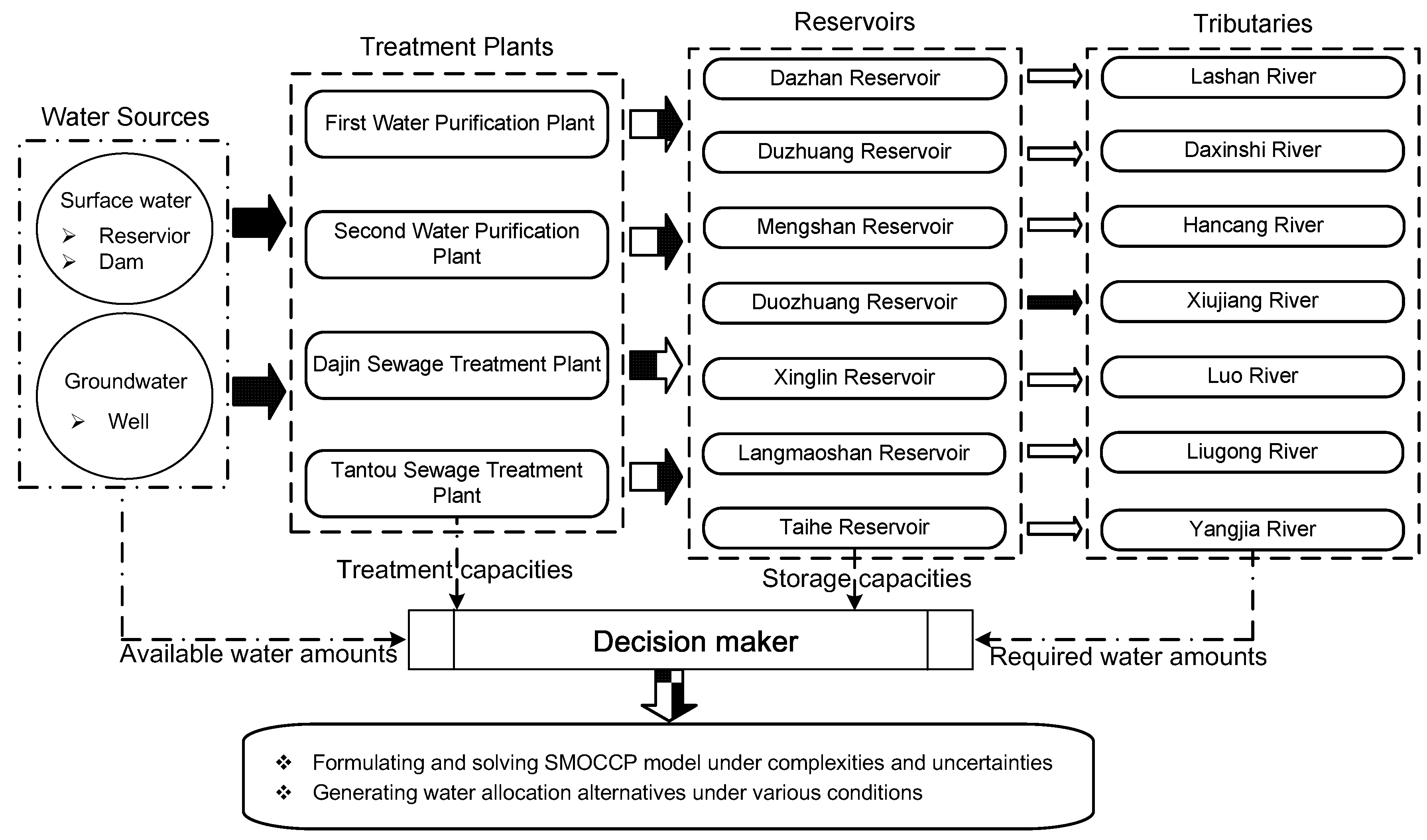
Figure 4.
Total transferred water amounts under various qi values.


Table 1.
The parameters related to water sources, treatment plants and reservoirs.
| Type | Item | System Parameters (×103 m3) | |
|---|---|---|---|
| Beginning Inventory | Maximum Capacities | ||
| Water source | Surface water | 19,000 | 2950 |
| Groundwater | 4200 | 3600 | |
| Treatment Plant | First Water Purification Plant | 7.5 | 1300 |
| Second Water Purification Plant | 13 | 2100 | |
| Dajin Sewage Treatment Plant | 0 | 10,000,000 | |
| Tantou Sewage Treatment Plant | 0 | 10,000,000 | |
| Reservoir | Dazhan Reservoir | 26 | 3150 |
| Duzhuang Reservoir | 13.5 | 580 | |
| Mengshan Reservoir | 3.5 | 185 | |
| Duozhuang Reservoir | 13.5 | 345 | |
| Xinglin Reservoir | 4.5 | 185 | |
| Langmaoshan Reservoir | 38 | 560 | |
| Taihe Reservoir | 6.5 | 345 | |
Table 2.
The hydraulic connection among the nodes of the water supply system.
| Type | Parameters | Item | ||||||
|---|---|---|---|---|---|---|---|---|
| r = 1 | r = 2 | r = 3 | r = 4 | r = 5 | r = 6 | r = 7 | ||
| t = 1 | transportation cost | 0 | 320 | 420 | 0 | 418 | 0 | 0 |
| leakage rate | 0 | 0.05 | 0.05 | 0 | 0.01 | 0 | 0 | |
| t = 2 | transportation cost | 0 | 220 | 0 | 222 | 315 | 350 | 110 |
| leakage rate | 0 | 0.05 | 0 | 0.03 | 0.03 | 0.07 | 0.01 | |
| t = 3 | transportation cost | 4400 | 1400 | 1350 | 530 | 0 | 0 | 0 |
| leakage rate | 0.51 | 0.25 | 0.25 | 0.08 | 0 | 0 | 0 | |
| t = 4 | transportation cost | 330 | 0 | 0 | 386 | 0 | 0 | 110 |
| leakage rate | 0.01 | 0 | 0 | 0.03 | 0 | 0 | 0.06 | |
| b = 1 | transportation cost | 580 | 0 | 0 | 0 | 0 | 0 | 0 |
| leakage rate | 0.45 | 0 | 0 | 0 | 0 | 0 | 0 | |
| b = 2 | transportation cost | 0 | 180 | 0 | 0 | 0 | 0 | 0 |
| leakage rate | 0 | 0.15 | 0 | 0 | 0 | 0 | 0 | |
| b = 3 | transportation cost | 0 | 0 | 180 | 0 | 0 | 0 | 0 |
| leakage rate | 0 | 0 | 0.10 | 0 | 0 | 0 | 0 | |
| b = 4 | transportation cost | 0 | 0 | 0 | 180 | 0 | 0 | 0 |
| leakage rate | 0 | 0 | 0 | 0.38 | 0 | 0 | 0 | |
| b = 5 | transportation cost | 0 | 0 | 0 | 0 | 180 | 0 | 0 |
| leakage rate | 0 | 0 | 0 | 0 | 0.15 | 0 | 0 | |
| b = 6 | transportation cost | 0 | 0 | 0 | 0 | 0 | 340 | 0 |
| leakage rate | 0 | 0 | 0 | 0 | 0 | 0.42 | 0 | |
| b = 7 | transportation cost | 0 | 0 | 0 | 0 | 0 | 0 | 180 |
| leakage rate | 0 | 0 | 0 | 0 | 0 | 0 | 0.05 | |
Notes: r is the index no. of the reservoirs; t is the index no. of the treatment plants; b is the index no. of the branches; 0 represents no hydraulic connections among the nodes.
Table 3.
System parameters over the twelve planning periods.
| Planning Period | Required Water Amounts (×103 m3) | Recovered Water Amounts (×103 m3) | |||||||
|---|---|---|---|---|---|---|---|---|---|
| b = 1 | b = 2 | b = 3 | b = 4 | b = 5 | b = 6 | b = 7 | Surface Water | Groundwater | |
| 1 | 6.10 m | 4.65 | 4.55 | 4.85 | 4.28 | 4.61 | 4.58 | 3172 | 629 |
| 0.63 s | 0.29 | 0.23 | 0.52 | 0.17 | 0.28 | 0.25 | |||
| 2 | 5.75 | 4.62 | 4.52 | 4.82 | 4.28 | 4.60 | 4.52 | 10,343 | 2059 |
| 0.75 | 0.25 | 0.21 | 0.49 | 0.15 | 0.26 | 0.21 | |||
| 3 | 5.34 | 4.62 | 4.52 | 4.82 | 4.28 | 4.60 | 4.52 | 14,359 | 2914 |
| 0.61 | 0.25 | 0.21 | 0.49 | 0.15 | 0.26 | 0.21 | |||
| 4 | 5.27 | 4.62 | 4.52 | 4.82 | 4.28 | 4.60 | 4.52 | 8492 | 1648 |
| 0.75 | 0.25 | 0.21 | 0.49 | 0.15 | 0.26 | 0.21 | |||
| 5 | 5.36 | 4.65 | 4.55 | 4.85 | 4.28 | 4.61 | 4.58 | 13,267 | 2676 |
| 0.59 | 0.29 | 0.23 | 0.52 | 0.17 | 0.28 | 0.25 | |||
| 6 | 5.35 | 4.70 | 4.61 | 4.90 | 4.29 | 4.63 | 4.61 | 16,782 | 3432 |
| 0.86 | 0.35 | 0.28 | 0.54 | 0.21 | 0.37 | 0.29 | |||
| 7 | 5.10 | 4.45 | 4.28 | 4.70 | 4.10 | 4.52 | 4.29 | 15,455 | 3169 |
| 0.81 | 0.32 | 0.21 | 0.35 | 0.14 | 0.21 | 0.20 | |||
| 8 | 5.34 | 4.62 | 4.52 | 4.82 | 4.28 | 4.60 | 4.52 | 11,782 | 2387 |
| 0.61 | 0.25 | 0.21 | 0.49 | 0.15 | 0.26 | 0.21 | |||
| 9 | 5.35 | 4.70 | 4.58 | 4.90 | 4.29 | 4.61 | 4.61 | 2606 | 541 |
| 0.78 | 0.35 | 0.25 | 0.54 | 0.20 | 0.29 | 0.28 | |||
| 10 | 5.47 | 4.80 | 4.61 | 5.00 | 4.32 | 4.65 | 4.65 | 225 | 65 |
| 0.75 | 0.40 | 0.29 | 0.54 | 0.20 | 0.40 | 0.40 | |||
| 11 | 5.47 | 4.75 | 4.61 | 5.00 | 4.31 | 4.65 | 4.63 | 239 | 53 |
| 0.67 | 0.37 | 0.28 | 0.54 | 0.20 | 0.40 | 0.37 | |||
| 12 | 5.51 | 4.72 | 4.60 | 4.90 | 4.31 | 4.63 | 4.61 | 74 | 56 |
| 0.40 | 0.37 | 0.26 | 0.54 | 0.20 | 0.37 | 0.29 | |||
Notes: b is the index no. of the branches; m represents the mean value of the log-normal distribution; s represents the standard deviation of the log-normal distribution.
Table 4.
Part of the solutions from the SMOCCP model under three constraint-violation levels at w1 = 0.9 and w2 = 0.1 (×103 m3).
Table 4.
Part of the solutions from the SMOCCP model under three constraint-violation levels at w1 = 0.9 and w2 = 0.1 (×103 m3).
| p | Transferred Path | k = 1 | k = 2 | k = 3 | k = 4 | k = 5 | k = 6 | k = 7 | k = 8 | k = 9 | k = 10 | k = 11 | k = 12 |
|---|---|---|---|---|---|---|---|---|---|---|---|---|---|
| 0.01 | S1→T1 | 2026.92 | 400.41 | 148.43 | 521.78 | 566.54 | 438.24 | 359.36 | 419.15 | 558.86 | 666.17 | 978.77 | 20.84 |
| S1→T2 | 4274.80 | 1514.01 | 48.12 | 48.13 | 48.23 | 2085.75 | 535.48 | 1622.93 | 1160.58 | 4042.63 | 101.58 | 0.19 | |
| S2→T4 | 3539.77 | 22,874.71 | 0.76 | 0.55 | 0.43 | 0.36 | 0.32 | 0.29 | 0.26 | 0.24 | 0.21 | 0.19 | |
| T1→R5 | 310.55 | 0.17 | 242.93 | 121.55 | 128.23 | 140.34 | 98.85 | 121.55 | 136.63 | 140.79 | 91.78 | 0.14 | |
| T2→R4 | 1049.58 | 651.13 | 295.46 | 651.13 | 707.83 | 785.01 | 407.88 | 651.13 | 785.01 | 867.57 | 867.57 | 785.01 | |
| T2→R6 | 915.28 | 341.22 | 341.22 | 93.06 | 0.00 | 722.87 | 0.00 | 943.37 | 363.59 | 494.48 | 339.48 | 0.17 | |
| T2→R7 | 180.19 | 506.52 | 154.35 | 0.00 | 0.00 | 557.01 | 122.25 | 12.20 | 0.37 | 540.15 | 0.00 | 208.53 | |
| T4→R1 | 3539.32 | 3283.20 | 1577.32 | 2021.45 | 1531.93 | 2864.25 | 1965.14 | 1577.32 | 2375.16 | 2475.19 | 2052.53 | 1155.28 | |
| R2→B2 | 240.15 | 215.08 | 215.08 | 215.08 | 240.15 | 288.58 | 213.04 | 215.08 | 288.58 | 364.58 | 320.05 | 310.59 | |
| R4→B4 | 686.59 | 631.59 | 631.59 | 631.59 | 686.59 | 761.46 | 395.64 | 631.59 | 761.46 | 841.54 | 841.54 | 761.46 | |
| R7→B7 | 184.89 | 156.46 | 156.46 | 156.46 | 184.89 | 206.44 | 121.03 | 156.46 | 200.99 | 280.76 | 253.98 | 206.44 | |
| 0.05 | S1→T1 | 1940.36 | 341.72 | 66.21 | 451.33 | 288.19 | 319.54 | 340.47 | 392.49 | 452.19 | 603.60 | 488.84 | 255.12 |
| S1→T2 | 3971.32 | 1248.16 | 0.00 | 0.01 | 0.11 | 1343.04 | 389.65 | 999.62 | 851.09 | 2856.74 | 0.35 | 0.19 | |
| S2→T4 | 2291.94 | 14,086.40 | 0.76 | 0.55 | 0.43 | 0.36 | 0.32 | 0.29 | 0.26 | 0.24 | 0.21 | 0.19 | |
| T1→R5 | 296.34 | 0.17 | 219.40 | 109.78 | 114.02 | 121.89 | 89.98 | 109.78 | 119.60 | 123.24 | 56.84 | 0.32 | |
| T2→R4 | 839.35 | 464.96 | 109.29 | 464.96 | 497.59 | 543.28 | 322.47 | 464.96 | 543.28 | 600.41 | 600.41 | 543.28 | |
| T2→R6 | 854.63 | 284.97 | 284.97 | 284.97 | 26.61 | 614.88 | 0.00 | 524.30 | 298.94 | 375.93 | 121.77 | 0.17 | |
| T2→R7 | 150.64 | 485.74 | 137.26 | 137.26 | 157.20 | 171.45 | 63.28 | 0.37 | 0.37 | 215.61 | 199.68 | 171.45 | |
| T4→R1 | 2291.48 | 1973.42 | 1041.50 | 1215.03 | 1027.50 | 1591.93 | 1135.82 | 1041.50 | 1394.48 | 1487.76 | 1303.23 | 878.31 | |
| R2→B2 | 197.44 | 181.04 | 181.04 | 181.04 | 197.44 | 228.16 | 171.09 | 181.04 | 228.16 | 277.17 | 249.11 | 241.74 | |
| R4→B4 | 482.67 | 451.01 | 451.01 | 451.01 | 482.67 | 526.98 | 312.80 | 451.01 | 526.98 | 582.40 | 582.40 | 526.98 | |
| R7→B7 | 155.63 | 135.88 | 135.88 | 135.88 | 155.63 | 169.73 | 105.94 | 135.88 | 166.55 | 213.45 | 197.68 | 169.73 | |
| 0.1 | S1→T1 | 1899.90 | 314.07 | 7.55 | 322.75 | 315.04 | 339.78 | 255.06 | 303.34 | 481.05 | 536.80 | 405.23 | 223.30 |
| S1→T2 | 3843.06 | 1123.63 | 0.00 | 0.01 | 0.11 | 839.73 | 317.66 | 878.60 | 723.41 | 2323.68 | 0.35 | 0.19 | |
| S2→T4 | 1816.46 | 10,904.65 | 0.76 | 0.55 | 0.43 | 0.36 | 0.32 | 0.29 | 0.26 | 0.24 | 0.21 | 0.19 | |
| T1→R5 | 289.42 | 0.17 | 207.80 | 103.98 | 107.09 | 113.06 | 85.58 | 103.98 | 111.41 | 114.80 | 40.12 | 0.32 | |
| T2→R4 | 754.13 | 388.56 | 32.89 | 388.56 | 412.37 | 446.49 | 284.51 | 388.56 | 446.49 | 493.45 | 493.45 | 446.49 | |
| T2→R6 | 826.66 | 256.45 | 261.32 | 258.89 | 265.37 | 304.62 | 0.00 | 480.88 | 269.31 | 324.83 | 27.13 | 0.17 | |
| T2→R7 | 136.84 | 475.81 | 127.32 | 127.32 | 143.41 | 154.46 | 29.97 | 0.37 | 0.37 | 186.30 | 174.71 | 154.46 | |
| T4→R1 | 1816.00 | 1504.45 | 834.78 | 926.29 | 830.46 | 1163.99 | 848.01 | 834.78 | 1049.86 | 1134.20 | 1022.99 | 758.92 | |
| R2→B2 | 177.88 | 165.15 | 165.15 | 165.15 | 177.88 | 201.30 | 152.22 | 165.15 | 201.30 | 239.49 | 217.96 | 211.51 | |
| R4→B4 | 400.00 | 376.90 | 376.90 | 376.90 | 400.00 | 433.09 | 275.98 | 376.90 | 433.09 | 478.64 | 478.64 | 433.09 | |
| R7→B7 | 141.97 | 126.05 | 126.05 | 126.05 | 141.97 | 152.91 | 98.68 | 126.05 | 150.68 | 184.44 | 172.96 | 152.91 |
Notes: p is the index of the probability levels; k is the index of months; S is the index of the water sources; T is the index of the treatment plants; R is the index of the reservoirs; B is the index of the tributaries.
Table 5.
Part of the solutions from the SMOCCP model under three constraint-violation levels at w1 = 0.1 and w2 = 0.9 (×103 m3).
Table 5.
Part of the solutions from the SMOCCP model under three constraint-violation levels at w1 = 0.1 and w2 = 0.9 (×103 m3).
| p | Transferred Path | k = 1 | k = 2 | k = 3 | k = 4 | k = 5 | k = 6 | k = 7 | k = 8 | k = 9 | k = 10 | k = 11 | k = 12 |
|---|---|---|---|---|---|---|---|---|---|---|---|---|---|
| 0.01 | S1→T1 | 921.66 | 2366.99 | 0.00 | 0.00 | 0.02 | 713.33 | 598.08 | 471.55 | 282.45 | 1071.53 | 0.06 | 679.81 |
| S1→T2 | 4227.46 | 504.30 | 145.88 | 0.00 | 0.00 | 0.00 | 0.00 | 263.33 | 205.07 | 785.94 | 758.62 | 662.47 | |
| S2→T4 | 3579.00 | 30,689.08 | 0.01 | 0.01 | 0.01 | 0.01 | 0.01 | 0.01 | 0.01 | 0.01 | 0.01 | 0.01 | |
| T1→R5 | 310.55 | 56.22 | 0.00 | 308.42 | 128.23 | 0.00 | 239.18 | 71.31 | 0.00 | 142.84 | 139.14 | 137.60 | |
| T2→R4 | 654.23 | 0.00 | 0.00 | 0.00 | 0.00 | 0.00 | 0.00 | 0.00 | 0.00 | 0.00 | 0.00 | 0.00 | |
| T2→R6 | 915.28 | 341.22 | 324.96 | 331.68 | 379.79 | 447.32 | 275.55 | 102.66 | 0.00 | 494.48 | 494.48 | 447.32 | |
| T2→R7 | 528.68 | 158.04 | 154.45 | 155.93 | 174.74 | 0.00 | 0.00 | 158.04 | 203.02 | 283.60 | 256.55 | 208.53 | |
| T4→R1 | 3539.32 | 3283.20 | 1577.32 | 2021.45 | 1531.93 | 2864.25 | 1965.14 | 1577.32 | 2375.16 | 2475.19 | 2052.53 | 1155.28 | |
| R2→B2 | 240.15 | 215.08 | 215.08 | 215.08 | 240.15 | 288.58 | 213.04 | 215.08 | 288.58 | 364.58 | 320.05 | 310.59 | |
| R4→B4 | 686.59 | 631.59 | 631.59 | 631.59 | 686.59 | 761.46 | 395.64 | 631.59 | 761.46 | 841.54 | 841.54 | 761.46 | |
| R7→B7 | 184.89 | 156.46 | 156.46 | 156.46 | 184.89 | 206.44 | 121.03 | 156.46 | 200.99 | 280.76 | 253.98 | 206.44 | |
| 0.05 | S1→T1 | 835.10 | 2284.77 | 0.00 | 0.00 | 0.02 | 277.48 | 626.91 | 305.46 | 172.92 | 882.87 | 0.06 | 554.48 |
| S1→T2 | 3475.50 | 136.05 | 0.00 | 0.00 | 0.00 | 0.00 | 0.00 | 426.50 | 243.39 | 217.79 | 581.42 | 524.86 | |
| S2→T4 | 2775.17 | 19,600.92 | 0.01 | 0.01 | 0.01 | 0.01 | 0.01 | 0.01 | 0.01 | 0.01 | 0.01 | 0.01 | |
| T1→R5 | 296.34 | 32.69 | 0.00 | 296.65 | 114.02 | 121.89 | 89.98 | 42.51 | 0.00 | 125.29 | 121.77 | 120.22 | |
| T2→R4 | 0.00 | 0.00 | 0.00 | 0.00 | 0.00 | 0.00 | 0.00 | 0.00 | 0.00 | 0.00 | 0.00 | 0.00 | |
| T2→R6 | 854.63 | 265.88 | 287.89 | 273.23 | 321.26 | 348.16 | 239.32 | 284.97 | 72.72 | 0.00 | 375.93 | 348.16 | |
| T2→R7 | 499.12 | 133.04 | 137.90 | 134.67 | 93.33 | 0.00 | 0.00 | 137.26 | 168.24 | 215.61 | 199.68 | 171.45 | |
| T4→R1 | 2291.48 | 1973.42 | 1041.50 | 1215.03 | 1027.50 | 1591.93 | 1135.82 | 1041.50 | 1394.48 | 1487.76 | 1303.23 | 878.31 | |
| R2→B2 | 197.44 | 181.04 | 181.04 | 181.04 | 197.44 | 228.16 | 171.09 | 181.04 | 228.16 | 277.17 | 249.11 | 241.74 | |
| R4→B4 | 482.67 | 451.01 | 451.01 | 451.01 | 482.67 | 526.98 | 312.80 | 451.01 | 526.98 | 582.40 | 582.40 | 526.98 | |
| R7→B7 | 155.63 | 135.88 | 135.88 | 135.88 | 155.63 | 169.73 | 105.94 | 135.88 | 166.55 | 213.45 | 197.68 | 169.73 | |
| 0.1 | S1→T1 | 794.64 | 2245.52 | 0.00 | 0.00 | 0.02 | 149.45 | 482.89 | 167.37 | 269.16 | 796.94 | 0.06 | 497.84 |
| S1→T2 | 3433.32 | 106.31 | 0.00 | 0.00 | 0.00 | 0.00 | 0.00 | 0.00 | 0.00 | 844.40 | 176.47 | 463.72 | |
| S2→T4 | 2214.48 | 15486.11 | 0.01 | 0.01 | 0.01 | 0.01 | 0.01 | 0.01 | 0.01 | 0.01 | 0.01 | 0.01 | |
| T1→R5 | 289.42 | 21.10 | 0.00 | 290.85 | 107.09 | 113.06 | 2.70 | 0.00 | 111.41 | 116.84 | 113.41 | 111.86 | |
| T2→R4 | 0.00 | 0.00 | 0.00 | 0.00 | 0.00 | 0.00 | 0.00 | 0.00 | 0.00 | 0.00 | 0.00 | 0.00 | |
| T2→R6 | 826.66 | 242.81 | 272.14 | 243.23 | 283.85 | 304.62 | 148.05 | 0.00 | 0.00 | 649.66 | 0.00 | 304.62 | |
| T2→R7 | 485.33 | 123.78 | 130.25 | 123.87 | 0.00 | 0.00 | 53.13 | 127.32 | 152.20 | 186.30 | 174.71 | 154.46 | |
| T4→R1 | 1816.00 | 1504.45 | 834.78 | 926.29 | 830.46 | 1163.99 | 848.01 | 834.78 | 1049.86 | 1134.20 | 1022.99 | 758.92 | |
| R2→B2 | 177.88 | 165.15 | 165.15 | 165.15 | 177.88 | 201.30 | 152.22 | 165.15 | 201.30 | 239.49 | 217.96 | 211.51 | |
| R4→B4 | 400.00 | 376.90 | 376.90 | 376.90 | 400.00 | 433.09 | 275.98 | 376.90 | 433.09 | 478.64 | 478.64 | 433.09 | |
| R7→B7 | 141.97 | 126.05 | 126.05 | 126.05 | 141.97 | 152.91 | 98.68 | 126.05 | 150.68 | 184.44 | 172.96 | 152.91 |
Notes: p is the index of the probability levels; k is the index of months; S is the index of the water sources; T is the index of the treatment plants; R is the index of the reservoirs; B is the index of the tributaries.
Table 6.
The demonstration of cost variation affecting the model solutions.
| P | Weighted Combination | Objective Function | Variation Levels of Targeted Parameters | ||||||
|---|---|---|---|---|---|---|---|---|---|
| −75% | −50% | −25% | 1 | +25% | +50% | +75% | |||
| 0.01 | w1 = 0.9 | TC (×106 RMB) | 12.89 | 25.78 | 38.67 | 51.56 | 64.46 | 77.35 | 90.24 |
| w2 = 0.1 | LL (×103 m3) | 19,055.62 | 19,055.62 | 19,055.62 | 19,055.62 | 19,055.62 | 19,055.62 | 19,055.62 | |
| w1 = 0.1 | TC (×106 RMB) | 13.50 | 27.01 | 40.51 | 54.01 | 67.51 | 81.01 | 94.51 | |
| w2 = 0.9 | LL (×103 m3) | 18,976.33 | 18,976.33 | 18,976.33 | 18,976.33 | 18,976.33 | 18,976.33 | 18,976.33 | |
| 0.05 | w1 = 0.9 | TC (×106 RMB) | 8.62 | 17.24 | 25.86 | 34.48 | 43.10 | 51.72 | 60.34 |
| w2 = 0.1 | LL (×103 m3) | 12,813.74 | 12,813.74 | 12,813.74 | 12,813.74 | 12,813.74 | 12,813.74 | 12,813.74 | |
| w1 = 0.1 | TC (×106 RMB) | 9.09 | 18.17 | 27.26 | 36.34 | 45.43 | 54.51 | 63.60 | |
| w2 = 0.9 | LL (×103 m3) | 12,753.19 | 12,753.19 | 12,753.19 | 12,753.19 | 12,753.19 | 12,753.19 | 12,753.19 | |
| 0.1 | w1 = 0.9 | TC (×106 RMB) | 7.01 | 14.01 | 21.02 | 28.02 | 35.03 | 42.03 | 49.04 |
| w2 = 0.1 | LL (×103 m3) | 10,440.01 | 10,440.01 | 10,440.01 | 10,440.01 | 10,440.01 | 10,440.01 | 10,440.01 | |
| w1 = 0.1 | TC (×106 RMB) | 7.39 | 14.79 | 22.18 | 29.57 | 36.96 | 44.36 | 51.75 | |
| w2 = 0.9 | LL (×103 m3) | 10,389.75 | 10,389.75 | 10,389.75 | 10,389.75 | 10,389.75 | 10,389.75 | 10,389.75 | |
Notes: TC is the abbreviation of the total costs; LL is the abbreviation of the leakage loss.
Table 7.
The demonstration of leakage rate variation affecting the model solutions
| P | Weighted Combination | Objective Function | Variation Levels of Targeted Parameters | ||||||
|---|---|---|---|---|---|---|---|---|---|
| −0.99% | −0.66% | −0.33% | 1 | 0.33% | 0.66% | 0.99% | |||
| 0.01 | w1 = 0.9 | TC (×106 RMB) | 51.19 | 51.32 | 51.44 | 51.56 | 51.69 | 51.81 | 51.94 |
| w2 = 0.1 | LL (×103 m3) | 18732.59 | 18839.74 | 18947.42 | 19055.62 | 19164.35 | 19273.62 | 19383.43 | |
| w1 = 0.1 | TC (×106 RMB) | 53.63 | 53.75 | 53.88 | 54.01 | 54.13 | 54.26 | 54.39 | |
| w2 = 0.9 | LL (×103 m3) | 18,654.29 | 18,761.11 | 18,868.46 | 18,976.33 | 19,084.73 | 19,193.66 | 19,303.14 | |
| 0.05 | w1 = 0.9 | TC (×106 RMB) | 34.24 | 34.32 | 34.40 | 34.48 | 34.56 | 34.64 | 34.72 |
| w2 = 0.1 | LL (×103 m3) | 12,598.37 | 12,669.82 | 12,741.60 | 12,813.74 | 12,886.22 | 12,959.05 | 13,032.23 | |
| w1 = 0.1 | TC (×106 RMB) | 36.09 | 36.17 | 36.26 | 36.34 | 36.43 | 36.51 | 36.60 | |
| w2 = 0.9 | LL (×103 m3) | 12,538.81 | 12,609.93 | 12,681.39 | 12,753.19 | 12,825.34 | 12,897.84 | 12,970.69 | |
| 0.1 | w1 = 0.9 | TC (×106 RMB) | 27.83 | 27.89 | 27.96 | 28.02 | 28.09 | 28.15 | 28.22 |
| w2 = 0.1 | LL (×103 m3) | 10,265.40 | 10,323.33 | 10,381.53 | 10,440.01 | 10,498.77 | 10,557.81 | 10,617.13 | |
| w1 = 0.1 | TC (×106 RMB) | 29.37 | 29.44 | 29.50 | 29.57 | 29.64 | 29.71 | 29.78 | |
| w2 = 0.9 | LL (×103 m3) | 10,215.96 | 10,273.62 | 10,331.54 | 10,389.75 | 10,448.23 | 10,507.00 | 10,566.04 | |
Notes: TC is the abbreviation of the total costs; LL is the abbreviation of the leakage loss.
© 2017 by the authors. Licensee MDPI, Basel, Switzerland. This article is an open access article distributed under the terms and conditions of the Creative Commons Attribution (CC BY) license (http://creativecommons.org/licenses/by/4.0/).
Share and Cite
MDPI and ACS Style
Xu, Y.; Li, W.; Ding, X. A Stochastic Multi-Objective Chance-Constrained Programming Model for Water Supply Management in Xiaoqing River Watershed. Water 2017, 9, 378. https://doi.org/10.3390/w9060378
AMA Style
Xu Y, Li W, Ding X. A Stochastic Multi-Objective Chance-Constrained Programming Model for Water Supply Management in Xiaoqing River Watershed. Water. 2017; 9(6):378. https://doi.org/10.3390/w9060378
Chicago/Turabian StyleXu, Ye, Wei Li, and Xiaowen Ding. 2017. "A Stochastic Multi-Objective Chance-Constrained Programming Model for Water Supply Management in Xiaoqing River Watershed" Water 9, no. 6: 378. https://doi.org/10.3390/w9060378
Note that from the first issue of 2016, this journal uses article numbers instead of page numbers. See further details here.