
LCA Methodology for the Quantification of the Carbon Footprint of the Integrated Urban Water System


School of Engineering and Architecture, University of Enna “Kore”, Cittadella Universitaria, Enna 94100, Italy
*
Author to whom correspondence should be addressed.
Water 2017, 9(6), 395; https://doi.org/10.3390/w9060395
Submission received: 31 March 2017
/
Revised: 23 May 2017
/
Accepted: 25 May 2017
/
Published: 2 June 2017
(This article belongs to the Special Issue Synergies in Urban Water Infrastructure Modeling)
Abstract
:In integrated urban water systems, energy consumption, and consequently the amount of produced CO2, depends on many environmental, infrastructural, and management factors such as supply water quality, on which treatment complexity depends, urban area orography, water systems efficiency, and maintenance levels. An important factor is related to the presence of significant water losses, which result in an increase in the supply volume and therefore a higher energy consumption for treatment and pumping, without effectively supplying users. The current European environmental strategy is committed to sustainable development by generating action plans to improve the environmental performance of products and services. The analysis of carbon footprints is considered one such improvement, allowing for the evaluation of the environmental impact of single production phases. Using this framework, the aim of the study is to apply a Life Cycle Assessment (LCA) methodology to quantify the carbon footprint of an overall integrated urban water system referring to ISO/TS 14067 (2013). This methodology uses an approach known as “cradle to grave” and presumes to conduct an objective assessment of product units, balancing energy, and matter flows along the production process. The methodology was applied to a real case study, i.e., the integrated urban water system of the Palermo metropolitan area in Sicily (Italy). Each process in the system was characterized and globally evaluated from the point of view of water loss, energy consumption, and CO2 production, and some mitigation strategies are proposed and evaluated to reduce the energy consumption and, consequently, the environmental impact of the system.
1. Introduction
The Intergovernmental Panel on Climate Change has highlighted the reciprocity between water efficiency and the mitigation of climate change; studies have demonstrated that water management policies have an influence on greenhouse gas (GHG) emissions and should be evaluated in terms of climate change mitigation [1,2,3]. The Carbon Footprint of Products (CFP) is a useful tool for this purpose. The first legislative reference available for the CFP was the PAS 2050 [4] (Publicly Available Specification), created in Britain in 2008 by the BSI (British Standards Institute) up to the standard ISO/TS 14067 published in May 2013. The ISO/TS 14067 defines the principles, requirements, and guidelines for the quantification and reporting of the Carbon Footprint, the quantification methodology, and the criteria for communication [5].
The Carbon FootPrint (CFP) is defined as “the total amount of greenhouse gas (GHG) emissions directly and indirectly caused by an activity or is accumulated over the life stages of a product” [6]. Typically, the calculation of the Carbon Footprint refers to the six GHGs identified in the Kyoto Protocol (CO2, CH4, N2O, SF6, HFCs, and PFCs) using the GWP (Global Warming Potential) of each, which represents the ratio between the heating caused by the specific GHG over a specific time interval and the heating caused over the same period by an equal amount of CO2 [7]. These calculations use the following formula:
where mi is the weight of the gases.
However, methodologies for the quantification of the carbon footprint are still evolving, and therefore definitions and calculations of carbon footprints are somewhat incoherent among studies due to disagreements regarding the selection of gases and the order of emissions to consider in footprint calculations [8]. The methodology suggested to quantify the CFP in the ISO/TS 14067 (2013) is the Life-Cycle Assessment (LCA). The LCA is an environmental management tool that evaluates the environmental performance of a service or a product using an evaluation of the emissions and consumption of resources at every stage of the life cycle, “from cradle to grave”. The LCA methodology plays a strategic role in identifying critical processes and potential improvement strategies for the urban water system. This is evident in numerous studies of water supply and transport systems, including Godskesen et al. [9], where the LCA approach was applied to evaluate three different water supply systems of the water sector in Copenhagen, Denmark, to evaluate the environmental impacts of each process involved; Del Borghi et al. [10], providing the analysis of potable water supply service in Sicily, Italy; Barjoveanu et al. [11], analysing the water services system in Iasi City (Romania) to demonstrate the usefulness of the LCA approach as a support tool for water resources management; and Sambito et al. [12], integrating the LCA approach with an analysis of the system energy and water balance in a water supply system. Other studies focused on urban drainage systems [13,14] and treatment plants [14,15]. More complete studies, like Jeong et al. [16], proposed an exhaustive analysis on environmental and human health impacts related to the integrated urban water cycle. It includes a comprehensive analysis of different impacts, providing lumped information on the whole system. The present study, keeping the focus on the integrated urban water system, is focused on water losses and energy consumption, analysing single sub-systems and parts of the integrated water cycle. With the present study, the water manager can investigate and improve single sub-systems and prioritise structural and non-structural measures to increase urban water service sustainability. A preliminary sensitivity analysis was carried out to address the selection of mitigation strategies.
The evaluation will have, as extreme borders, the water supply sources, from which the product unit (m3 of water) is abstracted to be supplied to users, and finally the discharge back to the environment, after being conveyed through the drainage system to the treatment plant.
2. Materials and Methods
2.1. Definition of the Objective and the Field of Application
The aim of the study is to evaluate the total greenhouse gas (GHG) emissions associated with the life cycle of potable water supplied to the urban users. The carbon footprint was quantified in accordance with the international standard ISO/TS 14067. The integrated water system considered in the study comprises the unit of abstraction and distribution of water, the drainage system, and a wastewater treatment plant, and the functional unit is 1 m3 of water delivered to users.
2.2. Inventory Analysis
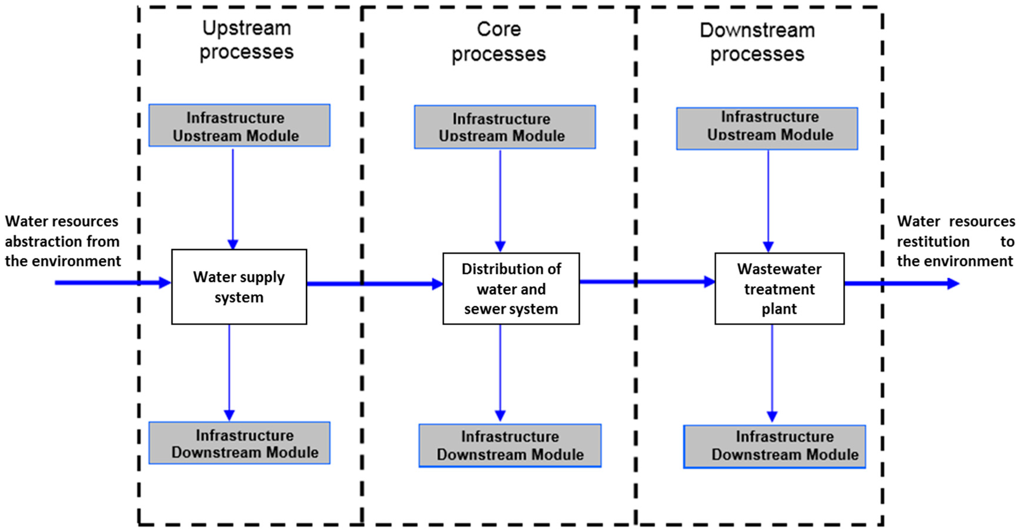
The system boundaries are defined in accordance with the PCR-UN CPC code 6921 [17] of the International EPD System (Environmental Product Declaration) and are represented in the Figure 1.
In the present study, the system boundaries include the following processes:
- Water supply and treatment system (upstream processes): including abstraction from natural sources, treatment plants, and transport to the metropolitan area
- Distribution of water and sewer system (core processes): including tanks, water distribution networks, and sewer networks
- Wastewater treatment plant (downstream processes)
The choices on system boundaries and life cycle phases taken in an LCA study on integrated water systems are very variable. Although Standardized guidelines employed to ensure the quality of the application of the LCA methodology would be necessary, Corominas et al. [18] highlights that since 1995, 45 international peer-reviewed papers dealing with WWT and LCA have been published in which, within the constraints of the ISO standards, there is a high variability in the definition of the functional unit and the system boundaries, in the selection of the impact assessment methodology, and in the procedure followed for interpreting the results. In this case, the phases referred to as the “infrastructure upstream module” and “infrastructure downstream module” (e.g., system construction and decommissioning phase) are not considered in the analysis as the system was implemented several years ago and this makes the evaluation of energy and the material fluxes connected with system implementation difficult and non-representative. The above choice is related to the aim of the paper to produce an operational tool to help the water manager to improve the current environmental management of the system, therefore considering only the system operating phase. The chemicals were not considered in the analysis as their consumption is only limited to potable water disinfection (wastewater treatment is entirely based on biological processes without the addition of chemicals) and their environmental impact is negligible with respect to the energy consumption along the integrated urban water system.
2.3. Case study
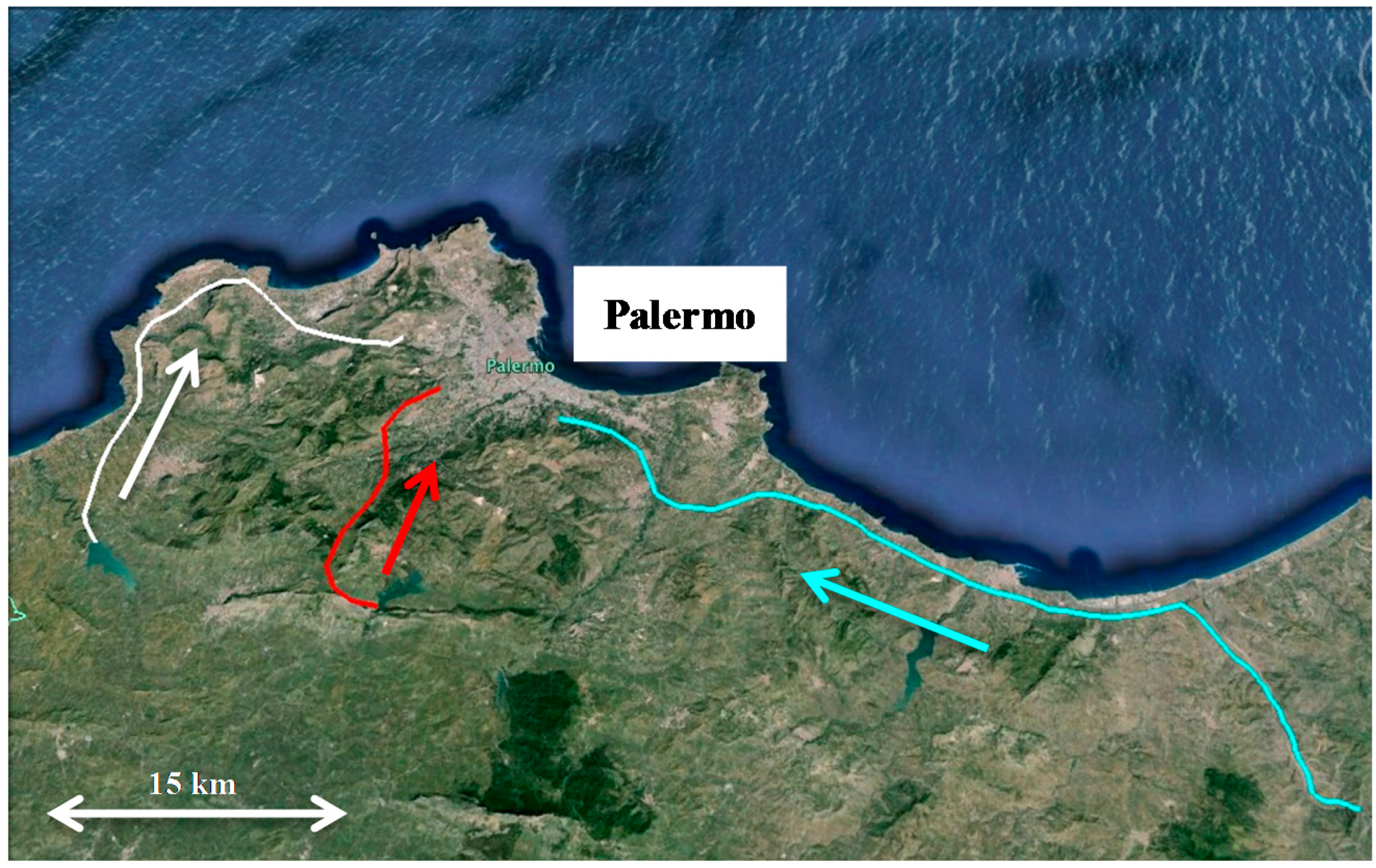
The city of Palermo is located on the northern coast of Sicily (Palermo); it has approximately 800,000 residents, 50,000 commuters, and 100,000 seasonal tourists (in summer). The city is surrounded to the north by the sea and in the other directions by mountains. Water is supplied by several ground (wells and springs) and surface (artificial reservoirs and rivers) sources. More specifically, the water sources are as follows:
- Four reservoirs (Scanzano, Piana degli Albanesi, Poma, and Rosamarina)
- Four groups of springs (Scillato, Presidiana, Risaiaimi, and Gabriele)
- Three river diversions (Imera, Oreto-S. Caterina, and Jato-Madonna del Ponte)
- Four groups of wells (Trabia, South Palermo, Oreto, and North Palermo)
Water is collected by three water subsystems (Figure 2): the Scillato system collects water from sources on the eastern side of the region; the Gabriele system collects water from sources in the southern mountains; and the Jato system collects water from sources on the western side of the region [19].
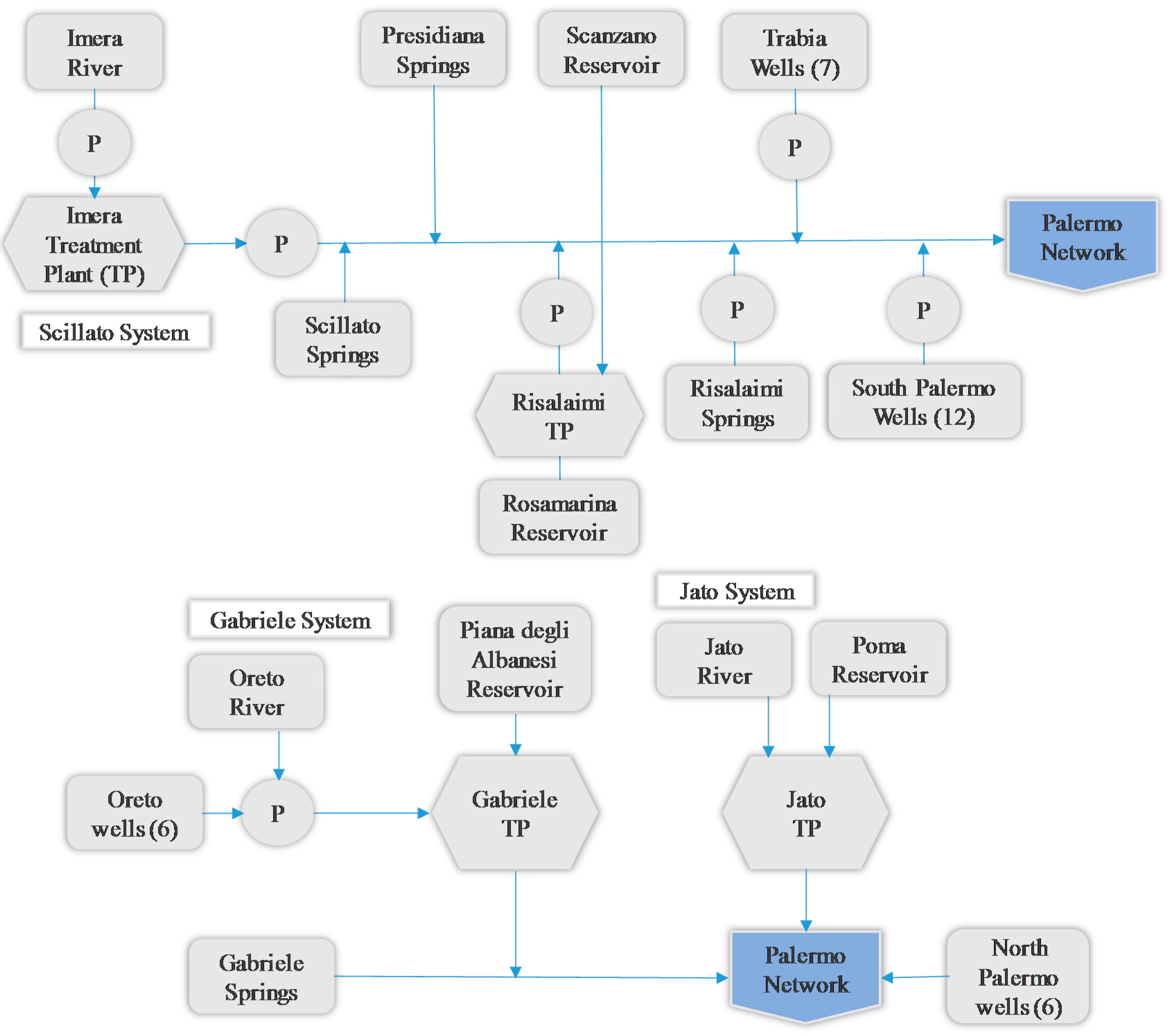
The Scillato system is the most complex, with three springs, 19 wells, two treatment plants (connected to three reservoirs), and six in-line pumping stations; it is also older than the other two supply systems, thus justifying the highest level of water losses. The Gabriele system is supplied by one spring, six wells, one treatment plant, and one inline pumping station. The Jato system is supplied by three wells and one treatment plant with no in-line pumps. Details of the system and the Palermo water supply can be found in Puleo et al. [18]. Data used in the present study are metred annual averages for 1997–2016.
Figure 3 shows a flow chart of the three systems, highlighting the water sources, pumping stations, and treatment plants.
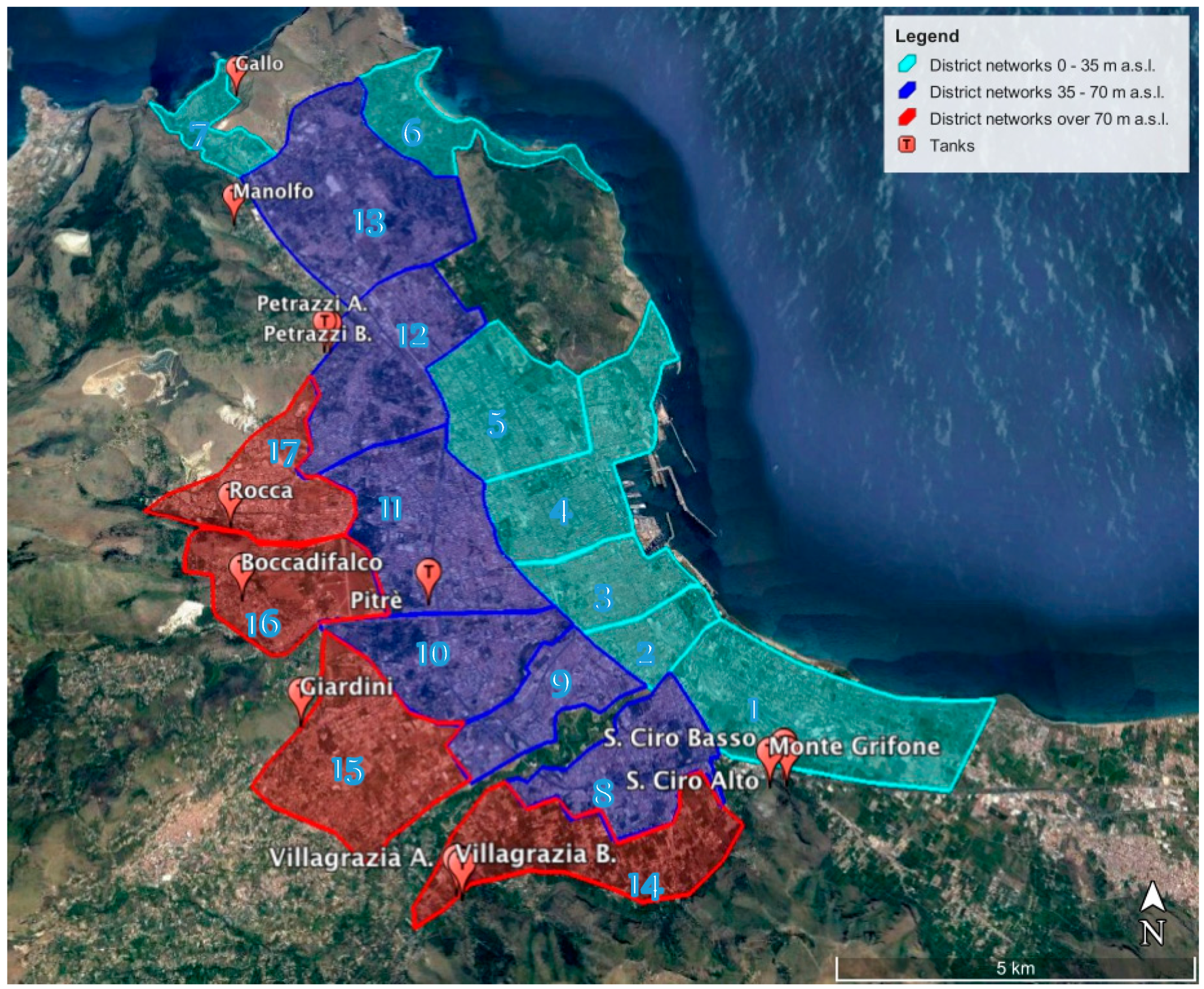
The water distribution network of the Palermo metropolitan area is divided into 17 districts with three pressure management areas based on ground elevation (0–35, 35–70, and over 70 m above sea level). Figure 4 shows the 17 districts and their reservoirs; Table 1 provides information on the average annual volumes billed to users, water losses, and energy consumption. The 10 pumping stations are positioned in correspondence to the tanks indicated in the figure.
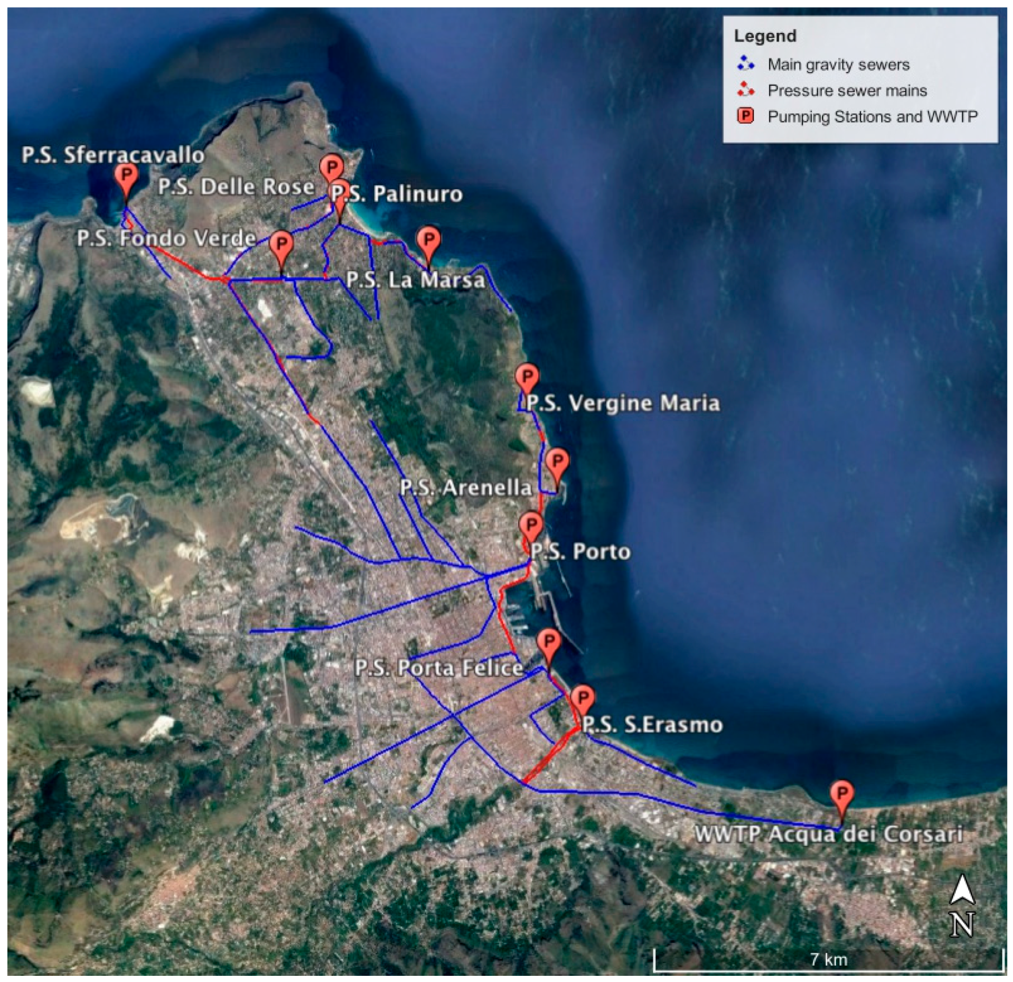
The analysed sewer system is combined: pipes are designed to carry the maximum wet weather flow for a specified return period; pumping stations and the wastewater treatment plant are designed against the sum of dry weather flows and the wet weather first flush (conventionally estimated as five times the average daily wastewater flow). The altimetry of the city and its significant coastal extension imposed the creation of three distinct drainage networks: one directly connected to the WWTP and the other two connected to pumping systems. Therefore, the urban area is divided into three major areas: one with delivery at the Porta Felice station, in the historic centre, and the other two with delivery to the Northeast at the Naval Shipyards. All pumping stations are interconnected to deliver sewage to the treatment plant. There are ten stations and their names and position are indicated in Figure 5.
The “Acqua dei Corsari” wastewater treatment plant is in the southern part of the city and is partially supplied by gravity sewers and pumping mains. The process scheme for the treatment plant is as follows: preliminary mechanical treatment for the removal of sand, grit, and a portion of the suspended solids; biological aeration to remove carbon and nutrients; and effluent disinfection before final discharge by means of an underwater outfall. The sludge from water treatment is sent on for thickening, aerobic digestion, and chemical and mechanical dewatering.
Water volumes, water losses, energy consumptions, and other data were collected thanks to the collaboration of the integrated water service manager of the 35 Municipalities of the Palermo Metropolitan Area.
2.4. Process Flow
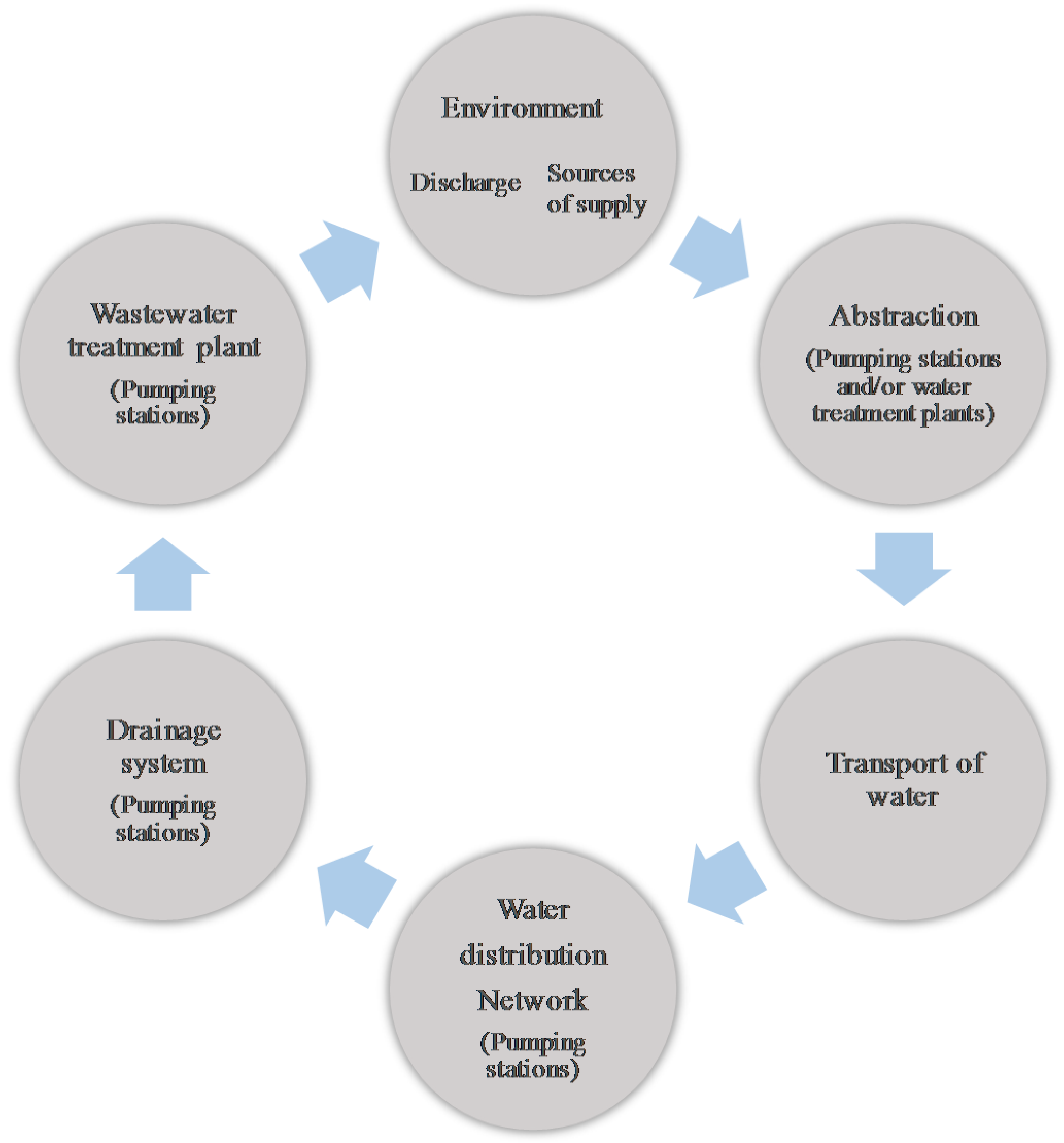
In the process flowchart below, the main processes and environmental interactions are identified through the representation of the components of a system with circles (processes sequences) linked by material flows (arrows). The main interactions are related to the flux of materials (water) from/to the environment and the energy consumption in all the phases of the process (Figure 6).
3. Results from the Current Scenario
In Palermo’s integrated water system, the average abstracted volume is 151.10 Mm3/year, and approximately 3.32 Mm3/year are exported to other systems directly at the source. The water volume supplied to the three supply systems (Scillato, Jato, and Gabriele) is thus equal to 147.78 Mm3/year (Table 1).
The average water loss in the three systems is approximately 27%; the Scillato water supply system is characterized by high losses (37.8%) due to the importance and complexity of the system and the larger number of deteriorated pipes; the Gabriele and Jato systems, of more recent construction than the Scillato system, are newer and characterized by lower leakage volumes (17.8% and 14%, respectively). The average water losses in each system are reported in Table 1.
The energy consumption in the Scillato system is mainly due to pumping: more than 70% of the total consumption is due to in-line pumps and wells. The energy consumption in the other two systems is mainly due to treatment, especially in the Jato system, which is characterized by gravity pipes in which pressure energy is not recovered.
According to the National Energy Authority, the carbon footprint for the Italian energy mix produces 0.527 kg CO2eq per kWh.
Figure 7 allows one to compare the amount of CO2eq produced and the extent of water loss in the three supply systems, which are the main factors responsible for the energy consumption of the systems. In Table 2, other details relating to the inflow and outflow volume, carbon footprint, and energy consumption with the total sum are presented.
As anticipated, the high level of leakages is also responsible for energy losses; more than 1.30 × 10⁷ kWh may potentially be saved yearly by eliminating leakages in the supply aqueducts, reducing GHG production by 689.84 t CO2eq per year.
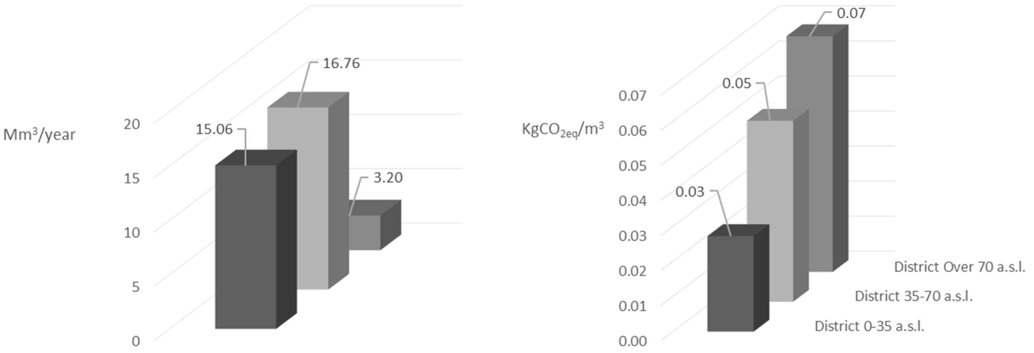
In the water distribution network, the annual average inflow volume is 107.71 Mm3/year. The network is divided into districts to limit the maximum pressure. Districts are the water volumes supplied to the subnets for the pressure band between 0–35 m a.s.l. (53.69 Mm3/year), 35–70 m a.s.l. (41.70 Mm3/year), and over 70 m a.s.l. (12.31 Mm3/year). The average water loss is approximately 32.5%: the subnets in the pressure area between 35–70 m a.s.l are characterized by high losses (40.19%); the pressure areas 0–35 m a.s.l. and over 70 m a.s.l. are characterized by newer distribution systems and lower leakage volumes (28.05% and 25.97%, respectively).
The energy consumption in the water distribution network is mainly due to pumping stations and is approximately 8 × 10⁶ kWh. Over 50% of the total consumption is from the subnet for the pressure band 35–70 m a.s.l., with 4.39 × 10⁶ kWh (Table 2).
As for the carbon footprint production, the two graphs shown in Figure 8 present the water losses and carbon footprint balance for the three districts. In Table 3, other details about the inflow and outflow volume and energy consumption for both the subnets and the entire water distribution network can be seen.
The sewer system of the city of Palermo pumps approximately 145.33 Mm3/year, and the sewage volume passing through the sewer system is around 88 million m3 (storm water is around 10 million m3), but considering the altimetry of the urban area, some of the volumes are pumped more than once, and the pumped volume is thus higher than the volume passing through the system to the wastewater treatment plant. The main energy consumption is due to the pumping stations; the pumping station with the highest energy consumption is Porta Felice, at 6.13 × 10⁶ kWh/year; the pumping station with the lowest energy consumption is La Marsa, at 7.85 × 10⁴ kWh/year. Consequently, the emission of GHG in the environment is mainly due to the presence of the pumping stations. Table 1 shows the water, energy, and carbon footprint balance of the system (Table 4).
The wastewater treatment plant “Acqua dei Corsari” receives the sewage water and storm water for a total of 98.42 Mm3/year. The treatment of these volumes involves an energy consumption and a relative production of CO2eq equal to the values indicated in Table 5.
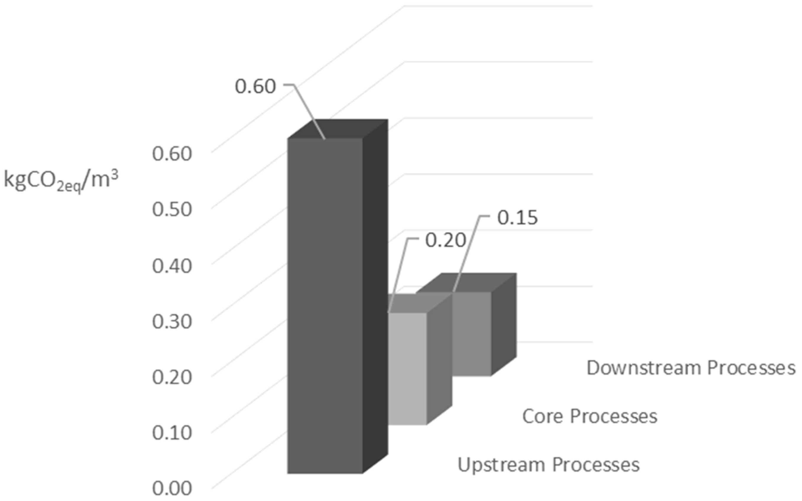
As shown in Figure 9, the carbon footprint produced per m3 of water supplied to users in the integrated water system, calculated using the LCA method, was in total: 0.95 kg CO2eq/m3, of which, 0.60 kg CO2eq/m3 was used for the upstream process (water supply), 0.20 kg CO2eq/m3 was used for the core process (water distribution and sewer network), and 0.15 kg CO2eq/m3 was used for the downstream process (wastewater treatment plant).
Comparing the carbon footprint of this case study with other case studies, we have noticed a significant variability with both higher and lower values. As the main driver of the carbon footprint increase in the urban water cycle is related to energy efficiency, this variability may depend on several aspects of the energy consumption (such as high level of leakages, the need for significant water treatment, and inefficient plants and pumping stations); in addition, the energy mix adopted at the national level (including sources such as coal, nuclear fission, natural gas, or renewable sources) may produce a different environmental impact of supplied energy. For example, in Barjoveanu et al. [11], the results have pointed out that the higher impacts are mainly due to the energetic effort needed for water supply abstraction and the fairly high water losses in the distribution system; for Jeong et al. [16], the electricity consumption is mainly due to water transport and treatment. In this case study, rather than water treatment, the greater energy consumption is to be attributed to the pumping stations and to the significant water volumes that need to be pumped to compensate for water losses.
4. Possible Mitigation Scenarios and Conclusions
Considering the complexity of the integrated water system, one possible scenario to improve the energy and environmental performance is to replace old pumps with high-efficiency pumps. The pumping stations are 30 years old, on average, and their efficiency is between 60% and 70%; new pumps and motors can reach efficiencies of 80–85%, thus reducing energy consumption.
In the water supply system, there are seven pumping stations with a starting performance ranging from 60–70%; therefore, the production of CO2eq undergoes an average reduction of 25%, from 0.21 to 0.16 kg CO2eq/m3. The effectiveness of the mitigation measure is certainly sensitive to the water supply volume and to its inter-annual variability. According to the available data in the period 1997–2016, the total annual supplied volume has a variation range equal to ±12% with respect to the average. This variability has a modest impact on unit CO2eq production ranging between 0.15 kg CO2eq/m3 and 0.17 kg CO2eq/m3 (±6.2% with respect to the average). The main reduction can be found in the Scillato system; the reduction is null in the Jato system because there are no pumping stations to be upgraded. The fact that the Jato system is unaffected by the mitigation measure reduces the sensitivity of CO2eq to water volume variability.
In the water distribution network, there are 10 pumping stations with a starting performance ranging from 65–75%. Therefore, the production of CO2eq undergoes a reduction of 14%, from 0.15 to 0.13 kg CO2eq/m3. The sensitivity of the result to water inflow volume variability is lower than 4% because pumping stations are mainly deputed to supply small groups of users with a high elevation.
In the sewer system, there are 10 pumping stations with a starting performance ranging from 65–75%. Therefore, the production of CO2eq undergoes a reduction of 12%, from 0.05 to 0.04 kg CO2eq/m3. Such a result is marginally affected by the collected volume inter-annual variability (equal to ±4 % with respect to the average according to the available dataset) and CO2eq production variation is limited to ±1.2% with respect to the average.
Another possible mitigation scenario related to the water system aims to reduce water losses. The Active Leakage Control (ALC) strategies aim at the prompt detection, localization, and repair of burst pipes, thus reducing possible damages and the volume of lost water. Using this, it is possible to reduce water losses to 10 %, resulting in a reduction in energy consumption and consequently in atmospheric pollution. In the case study, the CO2eq reduction was 6%, decreasing from 1.41 to 1.32 kg CO2eq/m3 per year.
Related to WWTP, a possible mitigation scenario relates to the transformation of sludge aerobic digestion to anaerobic processes that produce biogas. This involves the production of 24 kWh of energy per year for p.e. Consequently, there is a reduction in energy consumption and the quantity of the CO2eq. This case study showed a 60% reduction, from 0.15 to 0.06 kg CO2eq/m3 per year.
In conclusion, an evaluation of the system using the LCA methodology can define the amount of CFP units produced per m3 claimed. In the chosen case study, for the integrated water system of the city of Palermo (Sicily), with a defined objective and the field of applied analysis, it was possible to define the three parts of the life cycle: upstream, downstream, and core processes.
The results showed that the upstream processes, i.e., water supply and treatment system, gives rise to the more consistent portion of the CO2eq produced. Due to the presence of numerous pumping stations with low yields, it is the most energivorous. In second place is the upstream process, i.e., the water supply system, which in addition to having several pumping stations, is characterized by the presence of water treatment plants. Last is the downstream process, i.e., the wastewater treatment facility that contributes to the CFP. The analysis showed a certain sensitivity of the results to system variables, such as the supplied volume, and this fact may influence the reliability of mitigation strategies. In the future, uncertainty analysis approaches, frequently used in environmental analysis [12,20], should be introduced to increase the robustness of the analysis.
Author Contributions
The authors equally contributed to the present research and to the preparation of the paper.
Conflicts of Interest
The authors declare no conflict of interest.
References
- British Standardization Institution (BSI). PAS: 2050:2008: Specification for the Assessment of the Life Cycle Greenhouse Gas Emissions of Goods and Services, 1st ed.; BSI: London, UK, 2011. [Google Scholar]
- Savic, D.; Walters, G.; Schwab, M. Multiobjective genetic algorithms for pump schuduling in water supply. In Evolutionary Computing Workshop, AISB; Corne, D., Shapiro, J.L., Eds.; Springer: Manchester, UK, 1997; pp. 227–236. [Google Scholar]
- Olsson, G. Water and Energy: Threats and Opportunities; IWA Publishing: London, UK, 2012. [Google Scholar]
- Bates, B.C.; Kundzewicz, Z.W.; Wu, S.; Palutikof, J.P. Climate Change and Water; Technical Paper of the Intergovernmental Panel on Climate Change; IPCC Secretariat: Geneva, Switzerland, 2008; p. 210. [Google Scholar]
- International Standardization Organization ISO/TS 14067:2013. Greenhouse Gases—Carbon Footprint of Products—Requirements and Guidelines for Quantification and Communication, 1st ed.; International Organization for Standardization, ISO Central Secretariat: Geneva, Switzerland, 2013. [Google Scholar]
- Wiedmann, T.; Minx, J.A. Definition of “Carbon Footprint”. In Ecological Economics Research Trends; Pertsova, C.C., Ed.; Nova Science Publishers: Hauppauge, NY, USA, 2008. [Google Scholar]
- Laurent, A.; Olsen, S.I.; Hauschild, M.Z. Carbon footprint as environmental performance indicator for the manufacturing industry. CIRP Ann.-Manuf. Technol. 2010, 59, 37–40. [Google Scholar] [CrossRef]
- Pandey, D.; Agrawal, M.; Pandey, J.S. Carbon footprint: current methods of estimation. Environ. Monitor. Assess. 2011, 178, 135–160. [Google Scholar] [CrossRef] [PubMed]
- Godskesen, B.; Zambrano, K.C.; Trautner, A.; Johansen, N.B.; Thiesson, L.; Andersen, L.; Clauson-Kaas, J.; Neidel, T.L.; Rygaard, M.; Kløverpris, N.H.; et al. Life cycle assessment of three water systems in Copenhagen-a management tool of the future. Water Sci. Technol. 2011, 63, 565–572. [Google Scholar] [CrossRef] [PubMed]
- Del Borghi, A.; Strazza, C.; Gallo, M.; Messineo, S.; Naso, M. Water supply and sustainability: Life cycle assessment of water collection, treatment and distribution service. Int. J. Life Cycle Assess. 2013, 18, 1158–1168. [Google Scholar] [CrossRef]
- Barjoveanu, G.A.; Comandaru, I.M.; Rodriguez-Garcia, G.; Hospido, A.; Teodosiu, C. Evaluation of water services system through LCA. A case study for Iasi City. Int. J. Life Cycle Assess. 2014, 19, 449–462. [Google Scholar] [CrossRef]
- Sambito, M.; Puleo, V.; Freni, G. Energy, water and environmental balance of a complex water supply system. In 3rd International Conference on Water and Society; WIT Press: La Coruna, Spain, 2015; pp. 67–77. [Google Scholar]
- Lundin, M.; Morrison, G.M. A life cycle assessment based procedure for development of environmental sustainability indicators for urban water systems. Urban Water 2002, 4, 145–152. [Google Scholar] [CrossRef]
- Risch, E.; Gutierrez, O.; Roux, P.; Boutin, C.; Corominas, L. Life cycle assessment of urban wastewater systems: Quantifying the relative contribution of sewer systems. Water Res. 2015, 77, 35–48. [Google Scholar] [CrossRef] [PubMed]
- Benetto, E.; Nguyen, D.; Lohmann, T.; Schmitt, B.; Schosseler, P. Life cycle assessment of ecological sanitation system for small-scale wastewater treatment. Sci. Total Environ. 2009, 407, 1506–1516. [Google Scholar] [CrossRef] [PubMed]
- Jeong, H.; Minne, E.; Crittenden, J.C. Life cycle assessment of the City of Atlanta, Georgia’s centralized water system. Int. J. Life Cycle Assess. 2015, 20, 880–891. [Google Scholar] [CrossRef]
- Emilia-Romagna Development Agency (ERVET). Water Distribution through Mains, Except Steam and Hot Water; PCR—UN CPC Code 6921; Draft Version; ERVET: Stockholm, Sweden, 2011. [Google Scholar]
- Corominas, L.; Foley, J.; Guest, J.S.; Hospido, A.; Larsen, H.F.; Morera, S.; Shaw, A. Life cycle assessment applied to wastewater treatment: State of the art. Water Res. 2013, 47, 5480–5492. [Google Scholar] [CrossRef] [PubMed]
- Puleo, V.; Sambito, M.; Freni, G. An environmental analysis of the effect of energy saving, production and recovery measures on water supply systems under scarcity conditions. Energies 2015, 8, 5937–5951. [Google Scholar] [CrossRef]
- Dotto, C.B.S.; Mannina, G.; Kleidorfer, M.; Vezzaro, L.; Henrichs, M.; McCarthy, D.T.; Freni, G.; Rauch, W.; Deletic, A. Comparison of different uncertainty techniques in urban stormwater quantity and quality modelling. Water Res. 2012, 46, 2545–2558. [Google Scholar] [CrossRef] [PubMed]
Figure 1.
General system boundaries of the integrated urban water system.

Figure 2.
Water supply scheme in Palermo: Jato system (white); Gabriele System (red) and Scillato System (cyan).
Figure 2.
Water supply scheme in Palermo: Jato system (white); Gabriele System (red) and Scillato System (cyan).

Figure 3.
Schematic representation of the Scillato, Gabriele, and Jato systems: P represents pumping stations; TP represents treatment plants; and numbers in brackets are numbers of available wells.
Figure 3.
Schematic representation of the Scillato, Gabriele, and Jato systems: P represents pumping stations; TP represents treatment plants; and numbers in brackets are numbers of available wells.

Figure 4.
Districts and tanks in the water distribution network of Palermo.

Figure 5.
Diagram of the main sewer system and pumping station.

Figure 6.
Process flowchart of the integrated urban water system.

Figure 7.
Water losses (left) and carbon footprint balance (right) for the supply systems.
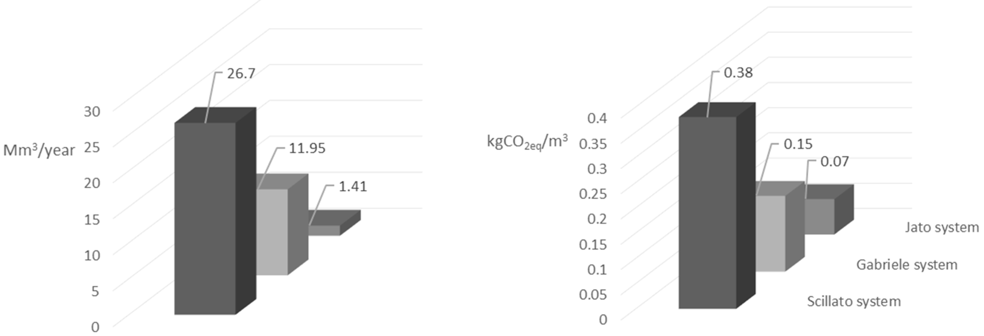
Figure 8.
Water losses (left) and carbon footprint balance (right) for the districts.

Figure 9.
The carbon footprint produced in the urban water system of the city of Palermo.


Table 1.
Main characteristics of district water distribution networks.
| N | District Water Distribution Networks | Tank | Annual Inflow | Annual Water Losses | Annual Energy Consumption |
|---|---|---|---|---|---|
| 0–35 m a.s.l. | [Mm3] | [Mm3] | [MWh] | ||
| 1 | Brancaccio-Romagnolo | S. Ciro Basso | 7.64 | 6.51 | - |
| 2 | Stazione | S. Ciro Alto | 2.48 | 0.37 | 605.93 |
| 3 | Centro Storico | Pitrè | 8.12 | 1.55 | - |
| 4 | Politeama | Pitrè | 12.93 | 2.14 | 678.75 |
| 5 | Libertà | Pitrè | 14.16 | 2.11 | 712.80 |
| 6 | Mondello | Petrazzi Basso | 7.36 | 2.08 | - |
| 7 | Sferracavallo | Gallo | 0.99 | 0.30 | - |
| Partial | 53.69 | 15.06 | 1997.48 | ||
| 35–70 m a.s.l. | |||||
| 8 | Giardini | Giardini | 0.38 | 0.12 | 325.12 |
| 9 | Bonagia | Montegrifone | 3.73 | 4.56 | 368.74 |
| 10 | Calatafimi | Montegrifone | 15.78 | 3.47 | 856.24 |
| 11 | Noce-Uditore | Petrazzi Alto | 10.59 | 2.02 | 1176.87 |
| 12 | Strasburgo-Cruillas | Petrazzi Alto | 8.21 | 4.12 | 1150.73 |
| 13 | T. Natale-Pallavicino | Petrazzi Alto | 3.02 | 2.47 | 512.37 |
| Partial | 41.70 | 16.76 | 4390.07 | ||
| Over 70 m a.s.l. | |||||
| 14 | Villa Adriana | Manolfo | 3.25 | 0.92 | 494.06 |
| 15 | Borgo Nuovo-Rocca | Rocca | 6.74 | 1.25 | 360.91 |
| 16 | Villagrazia | Villagr. A., B. | 1.74 | 0.82 | 192.72 |
| 17 | Boccadifalco | Boccadifalco | 0.59 | 0.21 | 576.41 |
| Partial | 12.32 | 3.20 | 1624.10 | ||
| Total | 107.71 | 35.02 | 8011.65 |
Table 2.
Inflow and outflow volume and energy consumption with the total sum.
| Unit | Scillato System | Gabriele System | Jato System | Total | |
|---|---|---|---|---|---|
| Inflow | Mm3/year | 70.65 | 67.03 | 10.10 | 147.78 |
| Outflow | Mm3/year | 43.94 | 55.07 | 8.68 | 107.71 |
| Carbon Footprint | kg CO2eq/m3 | 0.38 | 0.15 | 0.07 | 0.60 |
| Energy consumption | kWh | 2.83 × 10⁷ | 1.27 × 10⁷ | 1.32 × 10⁶ | 4.23 × 10⁷ |
Table 3.
Inflow and outflow volume and energy consumption for both the subnets and the entire water distribution network.
Table 3.
Inflow and outflow volume and energy consumption for both the subnets and the entire water distribution network.
| Unit | Pressure Area | Pressure Area | Pressure Area | Total | |
|---|---|---|---|---|---|
| 0–35 m a.s.l. | 35–70 m a.s.l. | over 70 m a.s.l. | |||
| Inflow | Mm3/year | 53.69 | 41.70 | 12.32 | 107.71 |
| Outflow | Mm3/year | 38.63 | 24.94 | 9.12 | 72.69 |
| Carbon Footprint | kg CO2eq/m3 | 0.03 | 0.05 | 0.07 | 0.15 |
| Energy consumption | kWh | 2.00 × 10⁶ | 4.39 × 10⁶ | 1.62 × 10⁶ | 8.01 × 10⁶ |
Table 4.
Water, energy, and carbon footprint balance of the sewage system.
| Unit | Total | |
|---|---|---|
| Pumped sewage volume | Mm3/year | 121.63 |
| Pumped storm water volume | MM3/year | 23.70 |
| Energy consumption | kWh/year | 1.33 × 10⁷ |
| Carbon footprint | kg CO2eq/m3 | 0.05 |
Table 5.
Water, energy, and carbon footprint balance of the wastewater treatment plant.
| Unit | Total | |
|---|---|---|
| Sewage volume | Mm3/year | 88.51 |
| Storm water volume | Mm3/year | 9.91 |
| Energy consumption | kWh/year | 2.76 × 10⁷ |
| Carbon footprint | kg CO2eq/m3 | 0.15 |
© 2017 by the authors. Licensee MDPI, Basel, Switzerland. This article is an open access article distributed under the terms and conditions of the Creative Commons Attribution (CC BY) license (http://creativecommons.org/licenses/by/4.0/).
Share and Cite
MDPI and ACS Style
Sambito, M.; Freni, G. LCA Methodology for the Quantification of the Carbon Footprint of the Integrated Urban Water System. Water 2017, 9, 395. https://doi.org/10.3390/w9060395
AMA Style
Sambito M, Freni G. LCA Methodology for the Quantification of the Carbon Footprint of the Integrated Urban Water System. Water. 2017; 9(6):395. https://doi.org/10.3390/w9060395
Chicago/Turabian StyleSambito, Mariacrocetta, and Gabriele Freni. 2017. "LCA Methodology for the Quantification of the Carbon Footprint of the Integrated Urban Water System" Water 9, no. 6: 395. https://doi.org/10.3390/w9060395
Note that from the first issue of 2016, this journal uses article numbers instead of page numbers. See further details here.