
Interannual and Decadal Variability in Tropical Pacific Sea Level


Department of Geosciences, University of Arizona, Tucson, AZ 85721, USA
*
Author to whom correspondence should be addressed.
Water 2017, 9(6), 402; https://doi.org/10.3390/w9060402
Submission received: 29 April 2017
/
Revised: 30 May 2017
/
Accepted: 2 June 2017
/
Published: 5 June 2017
(This article belongs to the Special Issue Sea Level Changes)
Abstract
:A notable feature in the first 20-year satellite altimetry records is an anomalously fast sea level rise (SLR) in the western Pacific impacting island nations in this region. This observed trend is due to a combination of internal variability and external forcing. The dominant mode of dynamic sea level (DSL) variability in the tropical Pacific presents as an east-west see-saw pattern. To assess model skill in simulating this variability mode, we compare 38 Coupled Model Intercomparison Project Phase 5 (CMIP5) models with 23-year satellite data, 55-year reanalysis products, and 60–year sea level reconstruction. We find that models underestimate variance in the Pacific sea level see-saw, especially at decadal, and longer, time scales. The interannual underestimation is likely due to a relatively low variability in the tropical zonal wind stress. Decadal sea level variability may be influenced by additional factors, such as wind stress at higher latitudes, subtropical gyre position and strength, and eddy heat transport. The interannual variability of the Niño 3.4 index is better represented in CMIP5 models despite low tropical Pacific wind stress variability. However, as with sea level, variability in the Niño 3.4 index is underestimated on decadal time scales. Our results show that DSL should be considered, in addition to sea surface temperature (SST), when evaluating model performance in capturing Pacific variability, as it is directly related to heat content in the ocean column.
1. Introduction
Gaining a better understanding of internal variability in the climate system is imperative for making more accurate predictions using climate models. Models must be able to simulate realistic internal variability before anthropogenically-induced long-term trends can be better detected [1]. On regional scales, sea-level variability can be caused by various factors such as winds, ocean currents, seawater density, and ocean mass distribution [2]. The magnitude of interannual and decadal sea level variability can be comparable to the long-term SLR signals [3,4,5]. Their combined effects are what coastal communities experience.
Previous work has been done to evaluate the ability of CMIP5 climate models in simulating both trends and internal variability in the Pacific, with focus on surface variables, such as SST and wind stress. SST variability in model simulations is found to be generally weaker than observed, especially at low latitudes and on decadal time scales [6]. The recent observed slowdown in the global mean surface temperature during 1998–2012 has been linked to stronger trade winds in the tropical Pacific that are not captured in climate model simulations [7]. This suggests that climate models may also underestimate wind stress variability in the tropical Pacific especially on decadal/interdecadal time scales [8]. Wind stress is directly related to DSL (i.e., sea surface height deviation from the geoid) and climate variability modes in the Pacific [9]. Unlike SST, DSL should be considered as an integrated quantity largely reflecting the total ocean heat storage in the tropical Pacific through the thermosteric effect.
It has also been shown that climate models tend to simulate interdecadal variability of SST more realistically than DSL, especially in the northwest tropical Pacific east of the Philippines [10]. In this critical region of anomalously fast sea level-rise, the rise rate can be modulated by decadal to multi-decadal variability related to the low frequency Southern Oscillation Index (SOI) and Pacific Decadal Oscillation (PDO) [11]. In general, CMIP5 models show improved performance over CMIP3 in the western tropical Pacific, but continue to show significant biases in both mean state and variability [12]. This currently presents a challenge in predicting future SLR especially for vulnerable island nations of this region.
In this study, we explore Pacific climate variability focusing on its manifestation on the sea level. To better understand the sources of model biases, we separate interannual and decadal DSL variability. Our work is focused in the region from 30° S to 45° N where an anomalously-fast SLR in the western Pacific has been observed during the satellite era [13]. In this region, interannual variability is dominated by El Niño/Southern Oscillation (ENSO) events. On longer time scales a combination of low-frequency ENSO and PDO are important [14]. We find that DSL variability is often underestimated in CMIP5 pre-industrial control simulations, suggesting that climate models may not reproduce the full range of potential regional SLR.
2. Materials and Methods
For our data-model comparison, we use satellite data, reanalysis, and a sea level reconstruction (Table 1). The satellite data offers an ideal comparison as it provides a precise global record of DSL, but is only available for 23 years. The additional historical products allow for a longer record with which to analyze the internal variability on interannual and decadal time scales. Reanalysis products combine observational data with a numerical model to produce a longer record of climate variables. Sea-level reconstruction is another method for extending the record, by combining tide-gauge observations altimetry data. As all datasets have strengths and weaknesses, we consider multiple products to help identify the most robust results.
For satellite altimetry data, we use the Archiving, Validation, and Interpretation of Satellite Oceanographic data (AVISO) with 1/4° × 1/4° resolution from January 1993 to December 2015 [15].
In addition to the relatively short observation data from AVISO, we also use three longer ocean and atmosphere climate reanalysis products:
- (1)
- (2)
- (3)
Long-term sea level variability and change have been reconstructed for the 20th century, derived from satellite altimetry combined with historical sea level measurements from tide gauges [22]. The reconstruction data span from 1950 to 2009 [23].
3. Results
We quantify DSL variability in the tropical Pacific using a see-saw index (SSI) [13]. The SSI is calculated as the difference of the mean DSL between the eastern (20° S–20° N, 160° W–100° W) and western (20° S–20° N, 120° E–180° E) tropical Pacific. The regions are chosen based on the DSL variability centers of the 1st empirical orthogonal function (EOF) in the AVISO and GFDL reanalysis products [13]. In the long-term mean, tropical Pacific sea level is tilted with the west higher than the east due to trade winds and water density differential (i.e., SSI is overall negative). Higher sea level anomalies in the western (eastern) Pacific correspond to more (less) negative SSI. The degree of tilt varies on interannual, decadal, and longer time scales related to ENSO, PDO, and other climate modes in the Pacific Ocean.
We evaluate model skill in capturing SSI variability by comparing CMIP5 pre-industrial control simulations with the AVISO data, the GFDL and ORAS4 reanalysis, and the sea level reconstruction—referred to collectively as historical products. Similar to the previous findings (i.e., Figure 2d in Peyser et al., 2016), the variability of the SSI as represented by its standard deviation is underestimated in the CMIP5 models. While most models also underestimate the mean, we do not find any correlation between the long-term mean SSI and its temporal variability (Figure 1).
To test the effect of external forcing on the SSI variability, we use historical and RCP8.5 simulations for a subset of the models, considering a sliding window of possible SSI standard deviations based on the length of the GFDL reanalysis. The results show that SSI variability in CMIP5 models is not significantly affected by external forcing. When record length is considered, there is a range of SSI variance over the shorter time windows, sometimes higher and sometimes lower than the variance of the entire record. In general, this range of variability cannot fully explain model underestimation. We believe that using the standard deviation over the entire record is a good metric for comparing the CMIP5 models to historical products containing 50+ years of data. However, with an even shorter record, the AVISO data may show greater variance if the past 23 years happened to be a period of particularly high variability.
The SSI standard deviation amongst the historical products ranges from 44mm (reconstruction) to 61 mm (AVISO) (Figure 1). Both reanalysis products show similar SSI variability with standard deviations of 50 mm (ORAS4) and 52 mm (GFDL). All CMIP5 models underestimate SSI standard deviation (values range from 14 mm to 48 mm) when compared to AVISO, ORAS4 reanalysis and GFDL reanalysis, with three models showing greater variability than the reconstruction.
To understand the source of the underestimation, we further separate the SSI variability into interannual and decadal/multi-decadal components using a low-pass filter. We choose a double-pass running mean filter with nine years as the cut-off for interannual variability. All lower-frequency variability will be referred to as decadal for this study. Using the filtered time series, we calculate interannual and decadal variance for SSI from the CMIP5 models and historical products. Due to the short record length of the AVISO data it is passed through the filter only once.
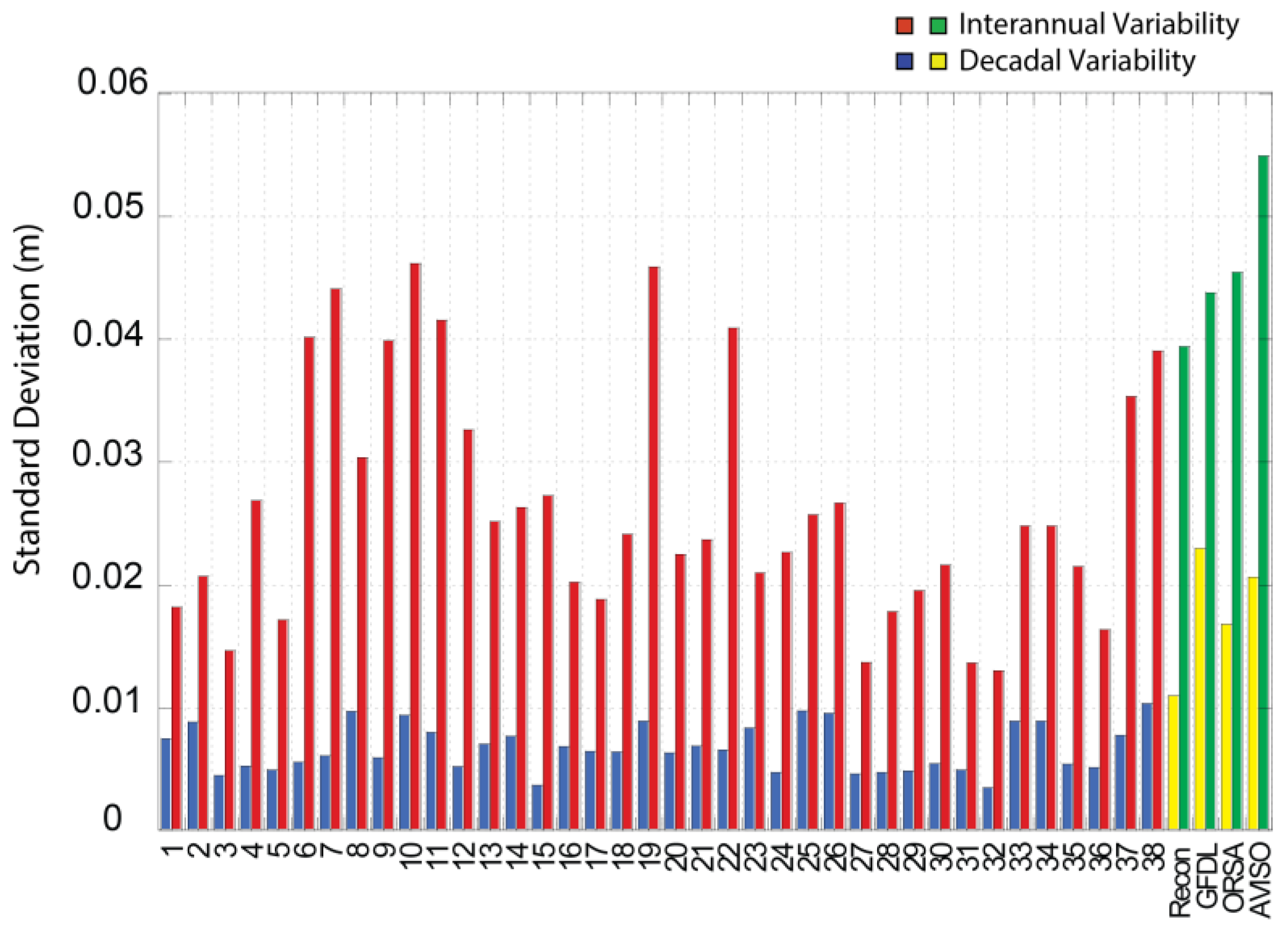
On interannual time scales, the model standard deviation spans from 13 mm to 46 mm (Figure 2). The historical products have SSI standard deviations ranging from 39 mm (reconstruction) to 55 mm (AVISO). Seven models show greater interannual SSI variability than the sea level reconstruction. All the models, including those that reproduce the observed magnitude of interannual variability well, underestimate the SSI variability on decadal time scales. The decadal model standard deviation ranges from 4 mm to 10 mm and the historical products from 11 mm to 23 mm. The correlation between interannual and decadal SSI standard deviation is low (0.41) with some models having better skills on decadal time scales and others most closely matching the historical products due to strong interannual variability. Most of the model-to-model difference in the total SSI variance stems from the interannual time scale.
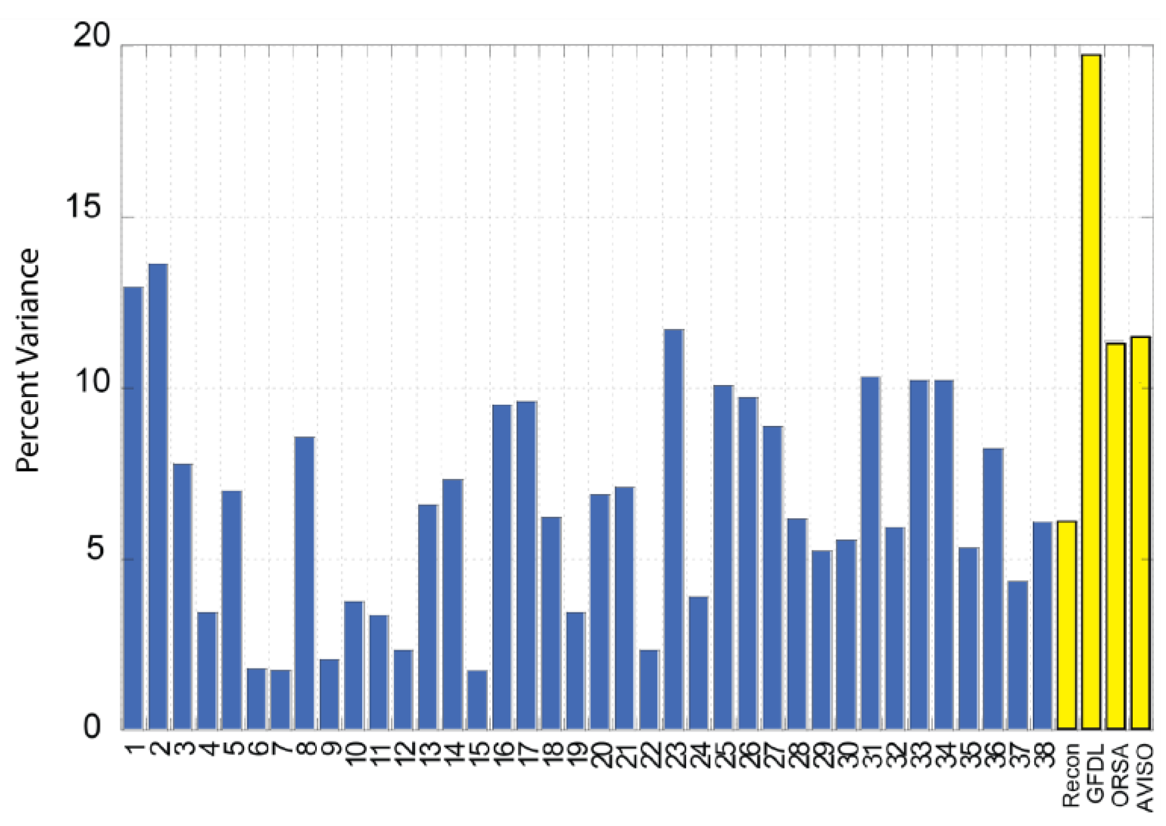
Another way to assess model skills is to consider the percentage of SSI variance due to variability on interannual and decadal time scales. We are interested to see if the models underestimate SSI across time scales or if models that reproduce total variance well have a breakdown that is different from what we see in the historical products. The GFDL reanalysis shows 20% of total SSI variance explained by decadal-scale variability. This is significantly higher than that in ORAS4 reanalysis (11%) and the sea level reconstruction (6%). The CMIP5 models show a range of 2% to 14% for the decadal component of variability (Figure 3). There are six models that show 10% or more of SSI variance due to decadal variability. These models are not necessarily the ones that best represent the total magnitude of variability. Some models, like Model #7 (Figure 2 and Figure 3) have skills in replicating interannual variability, but underestimate the percentage of total variance attributable to decadal time scales. Other models, like Model #2 (Figure 2 and Figure 3) show a percentage variance breakdown that is similar to the historical products, but underestimate the magnitude of both interannual and decadal variability.
We use the decomposed SSI index to determine the spatial patterns of DSL variability that occur on interannual and decadal time scales. To do that, we regress the interannual and decadal SSI time series to the DSL map for each of the CMIP5 models and historical products. We compare the multi-model ensemble mean with the GFDL reanalysis (Figure 4) and show the results for each individual model (Figure 5 and Figure 6).
In the GFDL reanalysis the Pacific sea level shows an ENSO-like pattern on interannual time scales (Figure 4a). When SSI is high (less negative) during an El Niño event, DSL is relatively high at the eastern equatorial Pacific and along the west coast of the Americas. In the tropics, this eastern high extends westward to 180° longitude and meridionally to 20° S and 20° N. During El Niño, DSL drops east of the Philippines and Indonesia. The CMIP5 ensemble mean shows a generally similar pattern with distinct differences in the interannual fingerprint (Figure 4b). The pattern also varies significantly between individual models (Figure 5). In many of the models, the eastern Pacific high seen during El Niño extends further into the western Pacific than is seen in the historical products. Another prevalent feature is an eastern high that covers a larger extent north to south. Some models also show distinct branches in the eastern high, north and south of the equator, that are not present in the historical products.
For the GFDL reanalysis the decadal sea level pattern is a clearly different from the fingerprint seen on interannual time scales. While there is still an east-west see-saw pattern, the eastern high does not extend as far west with the western low beginning at about 160° W. Some models, like Model #14, show a decadal pattern that is distinct from its interannual fingerprint, similar to the GFDL reanalysis However, in many of the CMIP5 models, the decadal SLR pattern is similar to the interannual pattern, like in Model #28.
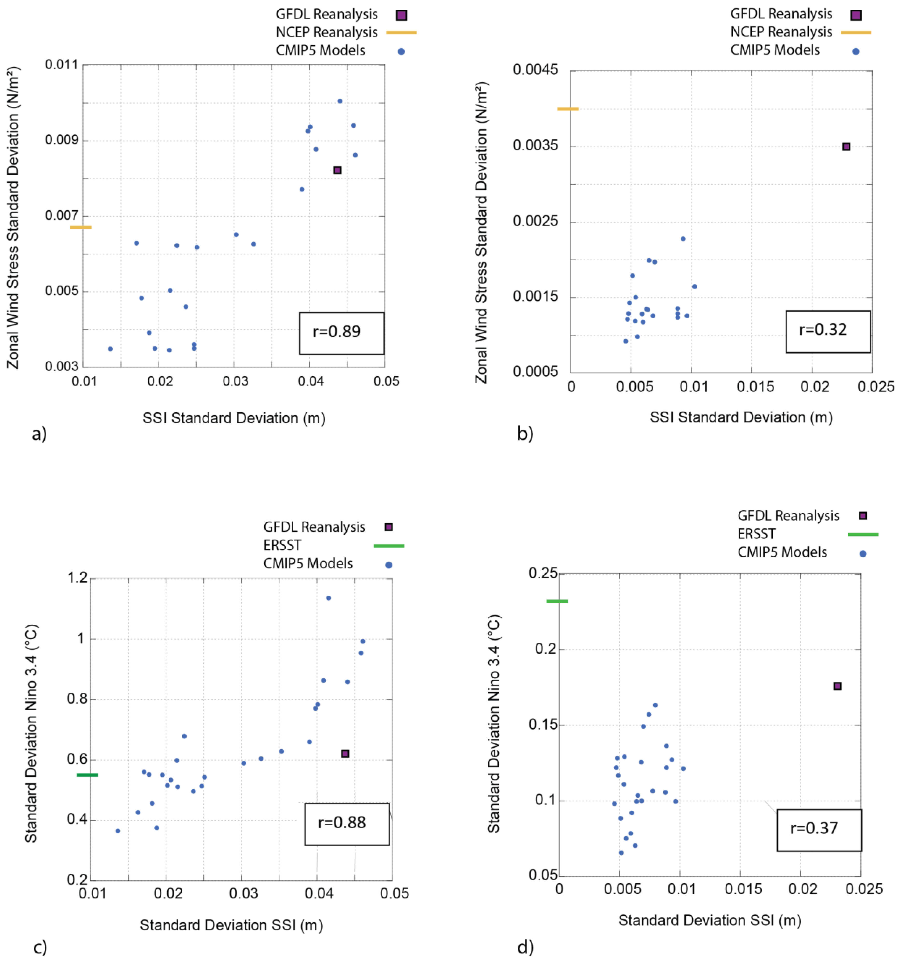
We examine the zonal wind stress in the climate models as a potential cause for the underestimation in sea level variability. We use the average zonal wind stress over the critical region 6° N–6° S and 180°–150° W based on the regression of the Interdecadal Pacific Oscillation (IPO) on wind stress [7]. We separate the zonal wind stress variability into interannual and decadal components using the same method as we did for the SSI. We use two Reanalysis products (GFDL and NCEP) for historical comparison with the CMIP5 models. On interannual time scales, the standard deviation is 8.2 × 10⁻³ N/m2 in GFDL and 6.7 × 10⁻³ N/m2 in NCEP/NCAR. The CMIP5 model standard deviation ranges from 3.5 × 10⁻³ N/m2 to 0.01 N/m2 with seven of the models showing greater zonal wind stress variability than the NCEP/NCAR reanalysis. There is a strong correlation (0.89) between the interannual standard deviation of tropical zonal wind stress and the standard deviation of the SSI across models (Figure 7a).
4. Discussion and Conclusions
When evaluating model skill in replicating SSI variability, we must consider the range of values found amongst the historical products. The two reanalysis datasets show greater SSI variability than the reconstruction on both interannual and decadal time scales. We chose to use this reconstruction because the cyclostationary empirical orthogonal function (CSEOF) method employed has been shown to better capture the historical ENSO signal than previous methods [22]. However, reconstructions are limited in their ability to show smaller-scale regional variability due to the limited spatial coverage provided by tide gauges, especially in the tropical Pacific. Temporally, they may not capture low-frequency variability due to the length of training data record [27]. We can expect the SSI interannual/decadal breakdown in AVISO to differ from the reanalysis due to the short length of the record and only being passed through the filter once. For these reasons, the reanalysis may provide a more accurate representation of regional variability in the Pacific, especially on decadal time scales. Lyu et al. [10] also show that reanalysis products have higher pattern correlations with CMIP5 models than sea level reconstruction on interdecadal time scales. Most differences between SSI in the two reanalyses occur in the early part of the record, where uncertainty is greatest.
We show that while CMIP5 models can capture many aspects in the climate system realistically, they systematically underestimate SSI variability, especially on decadal time scales. This result agrees with previous work on interdecadal Pacific variability [10]. The lack of correlation between the long-term mean SSI and its temporal variability suggests that a realistic pattern of the mean DSL in the models does not guarantee a proper simulation of DSL variability. There are distinct differences in the interannual sea level fingerprint between models, likely related to model differences in simulating ENSO. Known biases in CMIP5 representations of ENSO include a too-far-westward extent of the cold tongue and a double Intertropical Convergence Zone [28,29]. Therefore, to thoroughly evaluate model skill, both the pattern and magnitude of variability must be considered.
On interannual time scales, there is a direct relationship between tropical zonal wind standard deviation and SSI standard deviation across models. The high correlation suggests zonal wind stress could be the primary cause for the underestimation of interannual SSI variability. On decadal time scales, all CMIP5 models underestimate both SSI and tropical zonal wind variability. However, low correlation between these variables across models suggests that tropical wind stress (in the chosen region) cannot explain the decadal underestimation of SSI variability. Previous work has linked western Pacific sea level changes on decadal time scales to the North Pacific Gyre and the bifurcation latitude of the North equatorial current [30,31]. Wind forcing in the 12°–14° N band has a more significant influence on this bifurcation latitude than the Niño 3.4 index [32]. Therefore, our choice of region for tropical zonal wind stress would not capture this relationship. In addition to winds, mesoscale eddy forcing is important for explaining sea level changes in parts of the western Pacific, specifically in the Kuroshio Extension and Subtropical Countercurrent (STCC) regions [33,34]. Our western Pacific region used for calculating SSI includes these latitude bands (32°–38° N and 18°–28° N). As SSI considers sea level changes in both the western and eastern tropical Pacific, we expect it to be influenced by not only wind forcing, but also gyre and mesoscale eddy variability. Therefore, the choice of region, along with the inability of models to explicitly simulate small-scale features, explains why the decadal variability in tropical zonal wind stress has low correlation with SSI variability in our study.
The fact that all models underestimate interannual SSI variability, while still capturing the observed variability in interannual Niño 3.4, reinforces the importance of using sea level to truly represent Pacific climate variability. The CMIP5 models have shown significant improvement in simulating ENSO compared with the previous model generation (CMIP3), with some models slightly overestimating Niño 3.4 magnitude while the others slightly underestimate this variability [35]. The Niño 3.4 index considers only the surface ocean in the central to eastern Pacific, while SSI accounts for the subsurface in both the eastern and western Pacific. Therefore, underestimation of SSI variability suggests ocean heat content changes and western Pacific dynamics as potential areas of improvement in climate modelling. It is also interesting to note that Niño 3.4 variability is underestimated in all models at decadal time scales. As decadal ENSO variability has been shown to be affected higher latitudes, and these connections are a potential area for model improvement [36,37].
During the satellite era, island nations in the western Pacific have experienced SLR up to four times faster than the global mean rate of ~3 mm/year, while the sea level off the coast of North America has remained steady or even dropped slightly [5,38,39,40]. These observed trends are a combination of global SLR due to anthropogenic warming and internal variability, meaning they can change, with an increased rate in SLR off the coast of North America, when the Pacific sea level see-saw flips direction. Underestimation of Pacific sea level variability, especially on decadal time scales, is currently a bias in climate models. Our results suggest that, on interannual time scales, this is likely due to tropical zonal wind strength. Despite this, interannual Niño 3.4 variability is simulated well in CMIP5 models confirming the importance of SSI as an additional evaluation metric for model performance. On decadal time scales, the standard deviation of SSI, tropical zonal wind stress, and SST are all underestimated. This low frequency variability provides an important contribution to the observed trend in coastal SLR. For a more effective use of models to simulate future Pacific SLR, a realistic representation of interannual and decadal time scale variability is imperative for both surface and subsurface variables. Important areas of focus for model developers include: (1) western tropical Pacific dynamics (i.e., zonal wind stress and subtropical gyre strength and position); (2) mesoscale eddy heat transport (potentially improved by higher resolution models); and (3) interactions between the tropics and higher latitudes which can modulate decadal tropical variability. Advancements in this field will allow us to estimate the full range of potential SLR, which affects all those living in Pacific coastal regions.
Acknowledgments
This work is supported by NSF award #1513411. We thank the observation and modelling centers for making their data available.
Author Contributions
Cheryl E. Peyser and Jianjun Yin conceived and designed the study; Cheryl E. Peyser analyzed the data; Cheryl E. Peyser and Jianjun Yin wrote the paper.
Conflicts of Interest
The authors declare no conflict of interest.
References
- Deser, C.; Phillips, A.; Bourdette, V.; Teng, H. Uncertainty in climate change projections: the role of internal variability. Clim. Dyn. 2012, 38, 527–546. [Google Scholar] [CrossRef]
- Timmermann, A.; McGregor, S.; Jin, F.-F. Wind Effects on Past and Future Regional Sea Level Trends in the Southern Indo-Pacific. J. Clim. 2010, 23, 4429–4437. [Google Scholar] [CrossRef]
- Lyu, K.; Zhang, X.; Church, J.A.; Slangen, A.B.A.; Hu, J. Time of emergence for regional sea-level change. Nat. Clim. Chang. 2014, 11, 1006–1010. [Google Scholar] [CrossRef]
- Lyu, K.; Zhang, X.; Church, J.A.; Hu, J. Quantifying internally generated and externally forced climate signals at regional scales in CMIP5 models. Geophys. Res. Lett. 2015, 42, 2015GL065508. [Google Scholar] [CrossRef]
- Zhang, X.; Church, J.A. Sea level trends, interannual and decadal variability in the Pacific Ocean. Geophys. Res. Lett. 2012, 39, L21701. [Google Scholar] [CrossRef]
- Laepple, T.; Huybers, P. Global and regional variability in marine surface temperatures. Geophys. Res. Lett. 2014, 41, 2528–2534. [Google Scholar] [CrossRef]
- England, M.H.; McGregor, S.; Spence, P.; Meehl, G.A.; Timmermann, A.; Cai, W.; Gupta, A.S.; McPhaden, M.J.; Purich, A.; Santoso, A. Recent intensification of wind-driven circulation in the Pacific and the ongoing warming hiatus. Nat. Clim. Chang. 2014, 4, 222–227. [Google Scholar] [CrossRef]
- Lee, T.; Waliser, D.E.; Li, J.-L.F.; Landerer, F.W.; Gierach, M.M. Evaluation of CMIP3 and CMIP5 wind stress climatology using satellite measurements and atmospheric reanalysis products. J. Clim. 2013, 26, 5810–5826. [Google Scholar] [CrossRef]
- Landerer, F.W.; Gleckler, P.J.; Lee, T. Evaluation of CMIP5 dynamic sea surface height multi-model simulations against satellite observations. Clim. Dyn. 2014, 43, 1271–1283. [Google Scholar] [CrossRef]
- Lyu, K.; Zhang, X.; Church, J.A.; Hu, J. Evaluation of the interdecadal variability of sea surface temperature and sea level in the Pacific in CMIP3 and CMIP5 models. Int. J. Climatol. 2016, 36, 3723–3740. [Google Scholar] [CrossRef]
- Merrifield, M.A.; Maltrud, M.E. Regional sea level trends due to a Pacific trade wind intensification. Geophys. Res. Lett. 2011, 38, L21605. [Google Scholar] [CrossRef]
- Grose, M.R.; Brown, J.N.; Narsey, S.; Brown, J.R.; Murphy, B.F.; Langlais, C.; Gupta, A.S.; Moise, A.F.; Irving, D.B. Assessment of the CMIP5 global climate model simulations of the western tropical Pacific climate system and comparison to CMIP3. Int. J. Climatol. 2014, 34, 3382–3399. [Google Scholar] [CrossRef]
- Peyser, C.E.; Yin, J.; Landerer, F.W.; Cole, J.E. Pacific sea level rise patterns and global surface temperature variability. Geophys. Res. Lett. 2016, 43, 8662–8669. [Google Scholar] [CrossRef]
- Newman, M.; Alexander, M.A.; Ault, T.R.; Cobb, K.M.; Deser, C.; Di Lorenzo, E.; Mantua, N.J.; Miller, A.J.; Minobe, S.; Nakamura, H.; et al. The Pacific Decadal Oscillation, Revisited. J. Clim. 2016, 29, 4399–4427. [Google Scholar] [CrossRef]
- AVISO Satellite Altimetry Data. Available online: marine.copernicus.eu (accessed on 10 May 2017).
- Chang, Y.-S.; Zhang, S.; Rosati, A.; Delworth, T.L.; Stern, W.F. An assessment of oceanic variability for 1960–2010 from the GFDL ensemble coupled data assimilation. Clim. Dyn. 2013, 40, 775–803. [Google Scholar] [CrossRef]
- GFDL Data Portal. Available online: http://data1.gfdl.noaa.gov (accessed on 26 February 2017).
- Balmaseda, M.A.; Trenberth, K.E.; Källén, E. Distinctive climate signals in reanalysis of global ocean heat content. Geophys. Res. Lett. 2013, 40, 1754–1759. [Google Scholar] [CrossRef]
- ECMWF Ocean Reanalysis. Available online: http://www.ecmwf.int/en/research/climate-reanalysis/ocean-reanalysis (accessed on 10 January 2017).
- Kalnay, E.; Kanamitsu, M.; Kistler, R.; Collins, W.; Deaven, D.; Gandin, L.; Iredell, M.; Saha, S.; White, G.; Woollen, J.; et al. The NCEP/NCAR 40-Year Reanalysis Project. Bull. Am. Meteor. Soc. 1996, 77, 437–471. [Google Scholar] [CrossRef]
- NOAA Earth Systems Research Laboratory Physical Science Division. Available online: https://www.esrl.noaa.gov/psd/data/gridded/data.ncep.reanalysis.derived.html (accessed on 28 October 2016).
- Hamlington, B.D.; Leben, R.R.; Nerem, R.S.; Han, W.; Kim, K.-Y. Reconstructing sea level using cyclostationary empirical orthogonal functions. J. Geophys. Res. 2011, 116, C12015. [Google Scholar] [CrossRef]
- CCAR Reconstructed Sea Level Version 1. Available online: https://podaac.jpl.nasa.gov/dataset/RECON_SEA_LEVEL_OST_L4_V1 (accessed on 23 December 2016).
- Huang, B.; Banzon, V.F.; Freeman, E.; Lawrimore, J.; Liu, W.; Peterson, T.C.; Smith, T.M.; Thorne, P.W.; Woodruff, S.D.; Zhang, H.-M. Extended Reconstructed Sea Surface Temperature Version 4 (ERSST.v4). Part I: Upgrades and Intercomparisons. J. Clim. 2014, 28, 911–930. [Google Scholar] [CrossRef]
- Extended Reconstructed Sea Surface Temperature (ERSST), Version 4. Available online: https://data.nodc.noaa.gov/cgi-bin/iso?id=gov.noaa.ncdc:C00884 (accessed on 19 October 2016).
- CMIP5 - Coupled Model Intercomparison Project. Available online: http://cmip-pcmdi.llnl.gov/cmip5/ (accessed on 8 December 2016).
- Strassburg, M.W.; Hamlington, B.D.; Leben, R.R.; Kim, K.-Y. A comparative study of sea level reconstruction techniques using 20 years of satellite altimetry data. J. Geophys. Res. Oceans 2014, 119, 4068–4082. [Google Scholar] [CrossRef]
- Li, G.; Xie, S.-P. Tropical Biases in CMIP5 Multimodel Ensemble: The Excessive Equatorial Pacific Cold Tongue and Double ITCZ Problems. J. Clim. 2014, 27, 1765–1780. [Google Scholar] [CrossRef]
- Taschetto, A.S.; Gupta, A.S.; Jourdain, N.C.; Santoso, A.; Ummenhofer, C.C.; England, M.H. Cold Tongue and Warm Pool ENSO Events in CMIP5: Mean State and Future Projections. J. Clim. 2014, 27, 2861–2885. [Google Scholar] [CrossRef]
- Qiu, B.; Chen, S. Multidecadal Sea Level and Gyre Circulation Variability in the Northwestern Tropical Pacific Ocean. J. Phys. Oceanogr. 2012, 42, 193–206. [Google Scholar] [CrossRef]
- Lee, T.; McPhaden, M.J. Decadal phase change in large-scale sea level and winds in the Indo-Pacific region at the end of the 20th century. Geophys. Res. Lett. 2008, 35, L01605. [Google Scholar] [CrossRef]
- Qiu, B.; Chen, S. Interannual-to-Decadal Variability in the Bifurcation of the North Equatorial Current off the Philippines. J. Phys. Oceanogr. 2010, 40, 2525–2538. [Google Scholar] [CrossRef]
- Qiu, B.; Chen, S.; Wu, L.; Kida, S. Wind- versus Eddy-Forced Regional Sea Level Trends and Variability in the North Pacific Ocean. J. Clim. 2014, 28, 1561–1577. [Google Scholar] [CrossRef]
- Roemmich, D.; Gilson, J. Eddy Transport of Heat and Thermocline Waters in the North Pacific: A Key to Interannual/Decadal Climate Variability? J. Phys. Oceanogr. 2001, 31, 675–687. [Google Scholar] [CrossRef]
- Bellenger, H.; Guilyardi, E.; Leloup, J.; Lengaigne, M.; Vialard, J. ENSO representation in climate models: from CMIP3 to CMIP5. Clim. Dyn. 2014, 42, 1999–2018. [Google Scholar] [CrossRef]
- Lohmann, K.; Latif, M. Tropical Pacific Decadal Variability and the Subtropical–Tropical Cells. J. Clim. 2005, 18, 5163–5178. [Google Scholar] [CrossRef]
- Matei, D.; Keenlyside, N.; Latif, M.; Jungclaus, J. Subtropical Forcing of Tropical Pacific Climate and Decadal ENSO Modulation. J. Clim. 2008, 21, 4691–4709. [Google Scholar] [CrossRef]
- Bromirski, P.D.; Miller, A.J.; Flick, R.E.; Auad, G. Dynamical suppression of sea level rise along the Pacific coast of North America: Indications for imminent acceleration. J. Geophys. Res. 2011, 116, C07005. [Google Scholar] [CrossRef]
- Hamlington, B.D.; Strassburg, M.W.; Leben, R.R.; Han, W.; Nerem, R.S.; Kim, K.-Y. Uncovering an anthropogenic sea-level rise signal in the Pacific Ocean. Nat. Clim. Chang. 2014, 4, 782–785. [Google Scholar] [CrossRef]
- Han, W.; Meehl, G.A.; Hu, A.; Alexander, M.A.; Yamagata, T.; Yuan, D.; Ishii, M.; Pegion, P.; Zheng, J.; Hamlington, B.D.; et al. Intensification of decadal and multi-decadal sea level variability in the western tropical Pacific during recent decades. Clim. Dyn. 2014, 43, 1357–1379. [Google Scholar] [CrossRef]
Figure 1.
SSI mean and standard deviation for CMIP5 models compared against the historical products.
Figure 1.
SSI mean and standard deviation for CMIP5 models compared against the historical products.
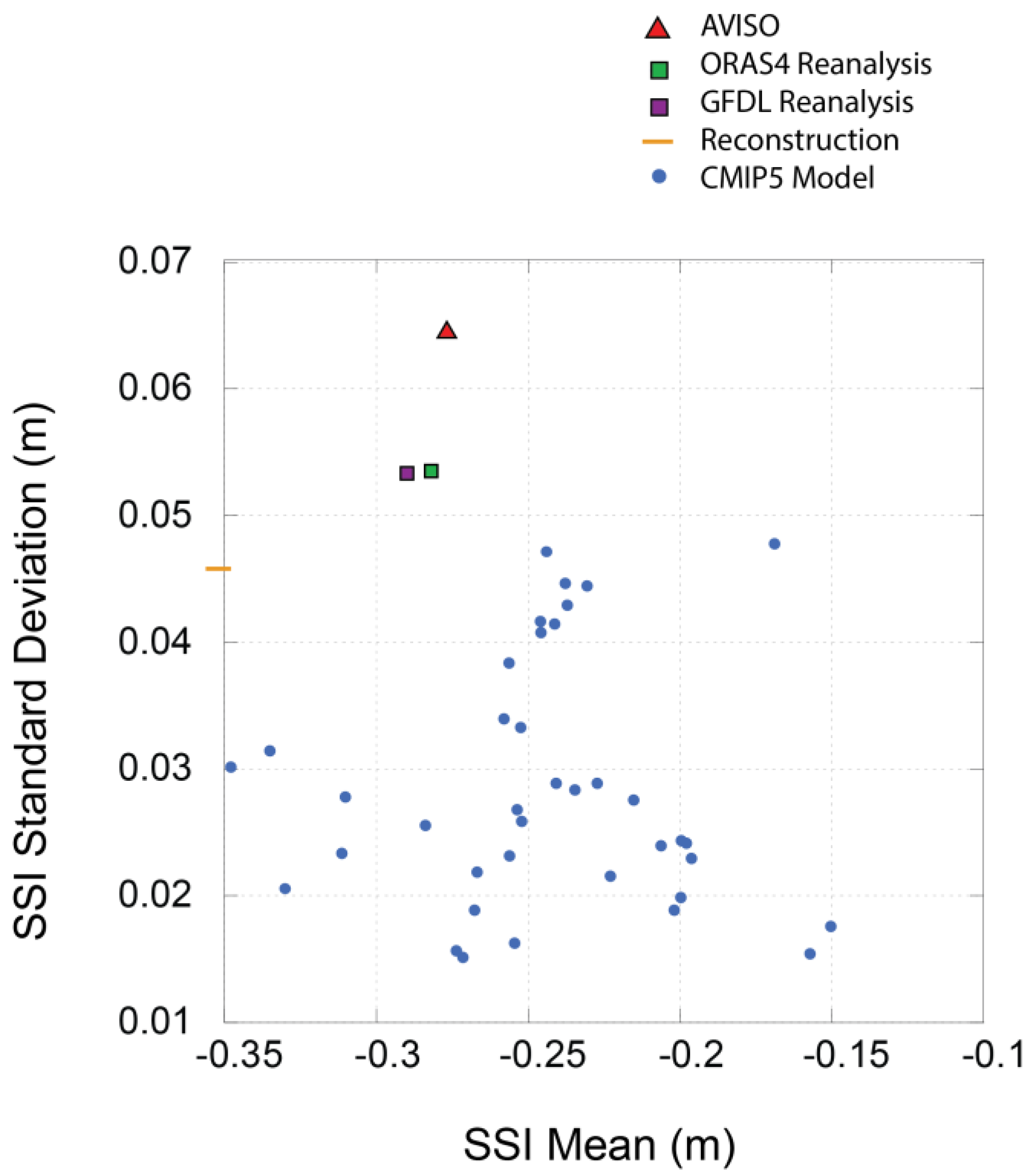
Figure 2.
SSI variability: interannual SSI standard deviation for CMIP5 models (red) and historical products (green); and decadal SSI standard deviation for models (blue) and historical products (yellow).
Figure 2.
SSI variability: interannual SSI standard deviation for CMIP5 models (red) and historical products (green); and decadal SSI standard deviation for models (blue) and historical products (yellow).

Figure 3.
Percent decadal SSI variability: percent SSI standard deviation due to decadal variability in CMIP5 models (blue) and historical products (yellow).
Figure 3.
Percent decadal SSI variability: percent SSI standard deviation due to decadal variability in CMIP5 models (blue) and historical products (yellow).

Figure 4.
Interannual and decadal DSL fingerprint: (a) Interannual GFDL Reanalysis; (b) Interannual CMIP5 ensemble mean; (c) Decadal GFDL Reanalysis; (d) Decadal CMIP5 ensemble mean. Spatial DSL is regressed to the SSI time series (meters of DSL/ meters of SSI). Red (blue) indicates DSL is high when interannual SSI index is high (low). The ensemble mean is calculated by performing the regression for each individual model, then averaging the results.
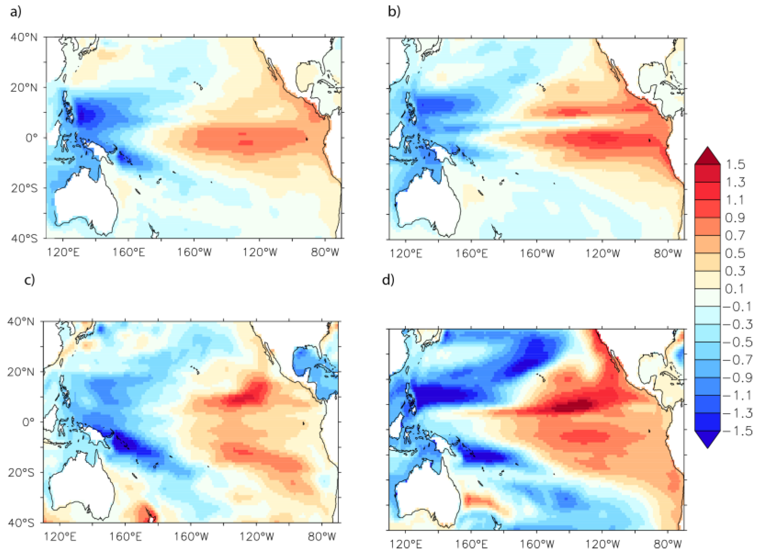
Figure 5.
Interannual sea level fingerprint: spatial DSL is regressed to SSI time series (meters of DSL/meters of SSI). Red (blue) indicates DSL is high when interannual SSI index is high (low). Numbered plots (1–38) represent individual CMIP5 models.
Figure 5.
Interannual sea level fingerprint: spatial DSL is regressed to SSI time series (meters of DSL/meters of SSI). Red (blue) indicates DSL is high when interannual SSI index is high (low). Numbered plots (1–38) represent individual CMIP5 models.
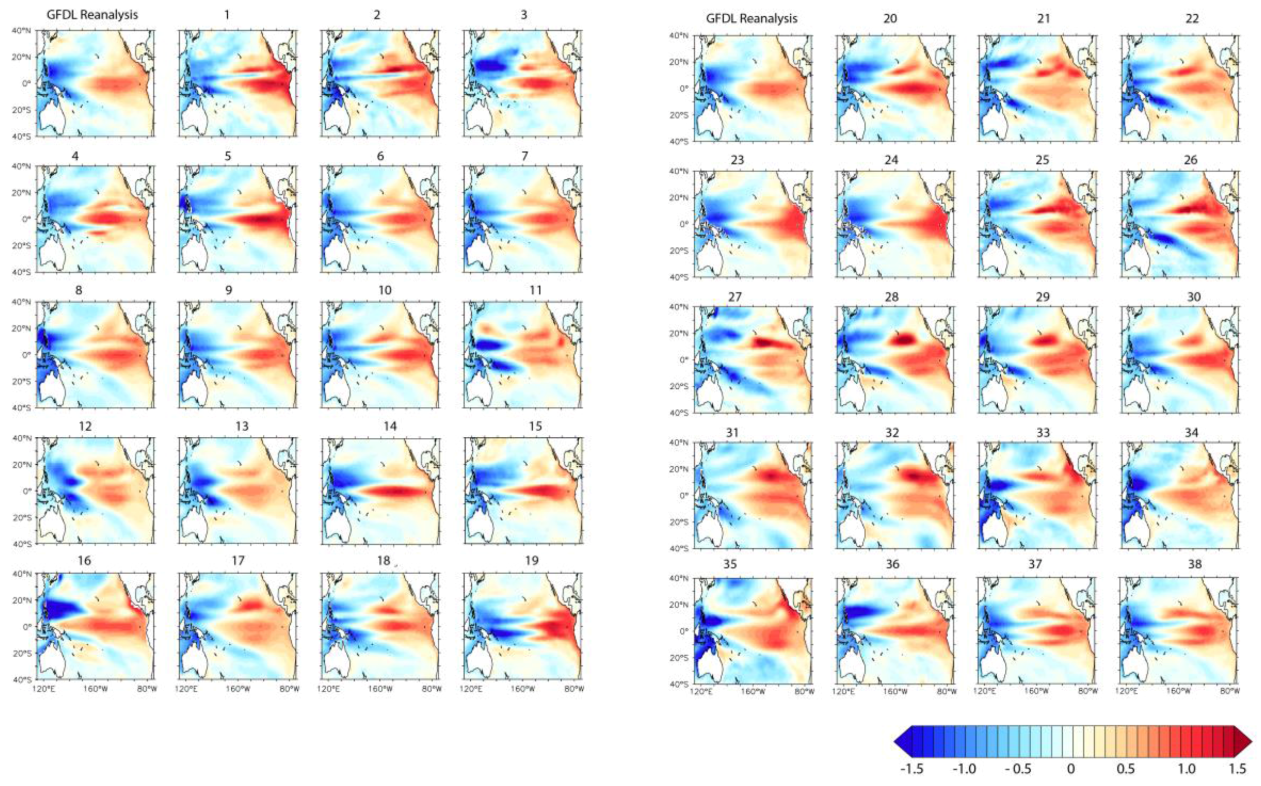
Figure 6.
Decadal sea level fingerprint: Spatial DSL is regressed to SSI time series (meters of DSL/meters of SSI). Red (blue) indicates DSL is high when decadal SSI index is high (low). Numbered plots (1–38) represent individual CMIP5 models.
Figure 6.
Decadal sea level fingerprint: Spatial DSL is regressed to SSI time series (meters of DSL/meters of SSI). Red (blue) indicates DSL is high when decadal SSI index is high (low). Numbered plots (1–38) represent individual CMIP5 models.
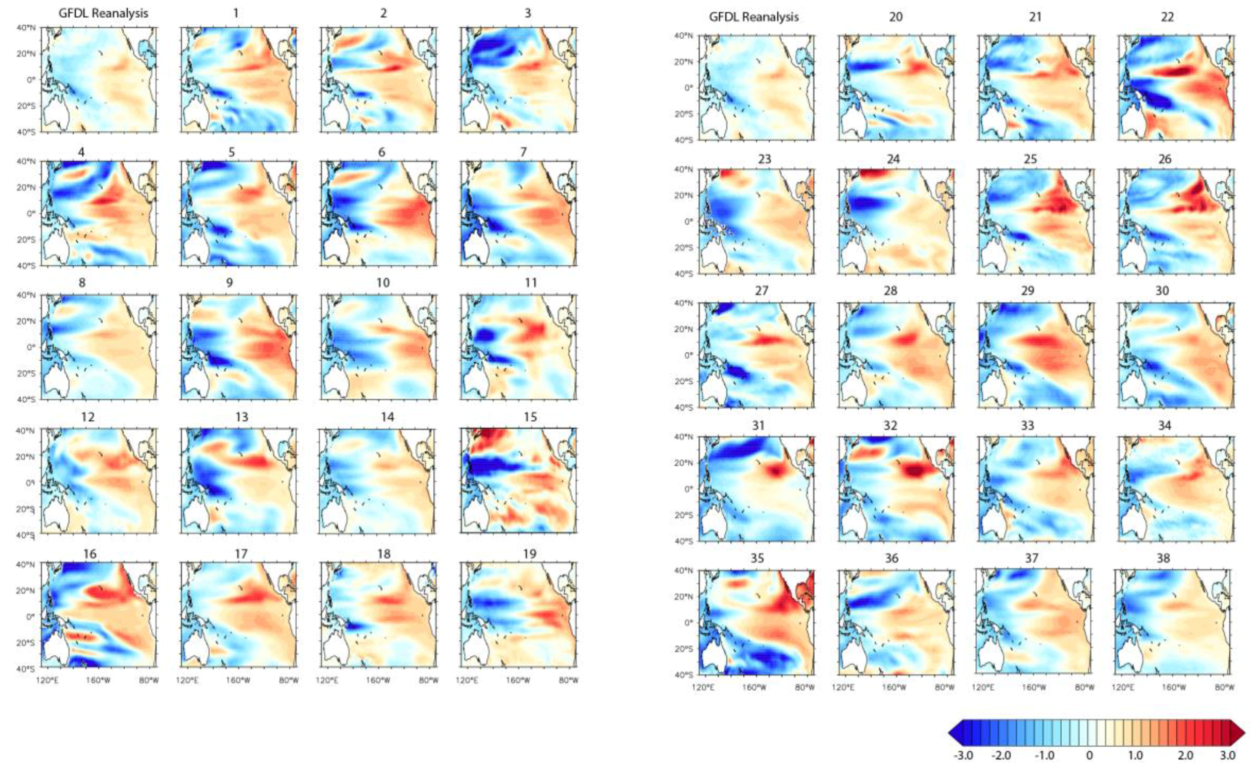
Figure 7.
(a,b) Average zonal wind stress (6° N–6° S and 180°–150° W) compared to SSI standard deviation in CMIP5 models and historical products for interannual (a) and decadal (b) time scales. (c,d) Standard deviation of average SST in Niño 3.4 region (120° W–170° W and 5° S–5° N) compared to SSI standard deviation in the CMIP5 models and historical products for interannual (c) and decadal (d) time scales. On decadal time scales the standard deviation is 3.5 × 10⁻³ N/m2 in GFDL and 4.1 × 10⁻³ N/m2 in NCEP. The CMIP5 models all underestimate decadal variability of the zonal winds compared to both reanalysis products with values ranging from 1–2 × 10⁻³ N/m2 (Figure 7b). The individual model time series show a relationship between zonal wind stress in this region and SSI on decadal scales. However, unlike interannual time scales, the standard deviation across models shows low correlation (0.32). Standard deviation of SSI on interannual time scales is also highly correlated (0.88) to SST in the Niño 3.4 region (Figure 7c). However, the interannual Niño3.4 index is not systematically underestimated in CMIP5 models the way DSL variability is. On decadal time scales the Niño 3.4 variability is underestimated in all models. However, Niño 3.4 decadal standard deviation is not well correlated (0.37) with SSI decadal standard deviation across models (Figure 7d).

Table 1.
Historical products.
| Data Set | Analysis Period | SSI | Wind Stress | SST |
|---|---|---|---|---|
| AVISO | 1993–2015 | x | ||
| GFDL Reanalysis | 1961–2015 | x | x | x |
| ORAS4 Reanalysis | 1958–2014 | x | ||
| Reconstruction | 1950–2009 | x | ||
| NCEP Reanalysis | 1948–2015 | x | ||
| ERSST | 1854–2014 | x |
Table 2.
CMIP5 models used. Two-hundred-year pre-industrial control simulations used. Models are chosen based on the availability in the CMIP5 archive at the time of download.
Table 2.
CMIP5 models used. Two-hundred-year pre-industrial control simulations used. Models are chosen based on the availability in the CMIP5 archive at the time of download.
| Model | SSI | Zonal Wind | SST | Model | SSI | Zonal Wind | SST | ||
|---|---|---|---|---|---|---|---|---|---|
| 1 | ACCESS1.0 | x | x | 20 | GFDL-CM3 | x | x | x | |
| 2 | ACCESS1.3 | x | x | 21 | GFDL-ESM2G | x | x | X | |
| 3 | BBC-CSM1.1 | x | 22 | GFDL-ESM2M | x | x | x | ||
| 4 | BBC-CSM1.1-m | x | 23 | GISS-E2R-CC | x | ||||
| 5 | CanESM2 | x | x | 24 | GISS-E2R | x | |||
| 6 | CCSM4.0 | x | x | x | 25 | HadGEM2-CC | x | ||
| 7 | CESM1-BGC | x | x | x | 26 | HadGEM2-ES | x | ||
| 8 | CESM1-CAM5 | x | x | x | 27 | INM-CM4 | x | x | x |
| 9 | CESM1-FASTCHEM | x | x | x | 28 | IPSL-CM5A-LR | x | x | |
| 10 | CESM1-WACCM | x | x | x | 29 | IPSL-CM5A-MR | x | x | |
| 11 | CMCC-CESM | x | x | x | 28 | IPSL-CM5B-LR | x | x | |
| 12 | CMCC-CMS | x | x | x | 31 | MIROC-ESM-CHEM | x | ||
| 13 | CMCC-CM | x | x | x | 32 | MIROC-ESM | x | ||
| 14 | CNRM-CM5 | x | 33 | MPI-ESM-LR | x | x | x | ||
| 15 | CNRM-CM5-2 | x | 34 | MPI-ESM-MR | x | x | x | ||
| 16 | CSIRO-Mk3.6.0 | x | x | 35 | MPI-ESM-P | x | x | x | |
| 17 | EC-EARTH | x | x | x | 36 | MRI-CGM3 | x | x | x |
| 18 | FGOALS_g2 | x | 37 | NorESM-M | x | x | |||
| 19 | FIO-ESM | x | x | 38 | NorESM-ME | x | x |
© 2017 by the authors. Licensee MDPI, Basel, Switzerland. This article is an open access article distributed under the terms and conditions of the Creative Commons Attribution (CC BY) license (http://creativecommons.org/licenses/by/4.0/).
Share and Cite
MDPI and ACS Style
Peyser, C.E.; Yin, J. Interannual and Decadal Variability in Tropical Pacific Sea Level. Water 2017, 9, 402. https://doi.org/10.3390/w9060402
AMA Style
Peyser CE, Yin J. Interannual and Decadal Variability in Tropical Pacific Sea Level. Water. 2017; 9(6):402. https://doi.org/10.3390/w9060402
Chicago/Turabian StylePeyser, Cheryl E., and Jianjun Yin. 2017. "Interannual and Decadal Variability in Tropical Pacific Sea Level" Water 9, no. 6: 402. https://doi.org/10.3390/w9060402
Note that from the first issue of 2016, this journal uses article numbers instead of page numbers. See further details here.