Modeling the Fate and Transport of Malathion in the Pagsanjan-Lumban Basin, Philippines

Abstract

Exposure to highly toxic pesticides could potentially cause cancer and disrupt the development of vital systems. Monitoring activities were performed to assess the level of contamination; however, these were costly, laborious, and short-term leading to insufficient monitoring data. However, the performance of the existing Soil and Water Assessment Tool (SWAT model) can be restricted by its two-phase partitioning approach, which is inadequate when it comes to simulating pesticides with limited dataset. This study developed a modified SWAT pesticide model to address these challenges. The modified model considered the three-phase partitioning model that classifies the pesticide into three forms: dissolved, particle-bound, and dissolved organic carbon (DOC)-associated pesticide. The addition of DOC-associated pesticide particles increases the scope of the pesticide model by also considering the adherence of pesticides to the organic carbon in the soil. The modified SWAT and original SWAT pesticide model was applied to the Pagsanjan-Lumban (PL) basin, a highly agricultural region. Malathion was chosen as the target pesticide since it is commonly used in the basin. The pesticide models simulated the fate and transport of malathion in the PL basin and showed the temporal pattern of selected subbasins. The sensitivity analyses revealed that application efficiency and settling velocity were the most sensitive parameters for the original and modified SWAT model, respectively. Degradation of particulate-phase malathion were also significant to both models. The rate of determination (R²) and Nash-Sutcliffe efficiency (NSE) values showed that the modified model (R² = 0.52; NSE = 0.36) gave a slightly better performance compared to the original (R² = 0.39; NSE = 0.18). Results from this study will be able to aid the government and private agriculture sectors to have an in-depth understanding in managing pesticide usage in agricultural watersheds.

1. Introduction

Agriculture has been substantial to the Philippine economy and has contributed 10.2% to 13.2% of the country’s GDP in the past decade [1]. To keep up with this demand, various kinds of pesticides were applied to different crops and vegetables to help increase food supplies and provide greater revenue for farmers. However, exposure to pesticides could potentially cause cancer and disrupt the development of vital systems (endocrine, reproductive, and immune systems) [2,3,4]. Pesticide contamination in soil and water also has negative effects on the diversity of the flora and fauna of local areas thereby disturbing the existing ecosystem [5,6,7]. Various kinds of pesticides are used in agriculture depending on the target pests. Hence, many kinds of chemicals exist and find their way into the groundwater, surface water, soils, and eventually drinking water [8,9,10,11]. Several attempts have been made to monitor and map out their potential areas of contamination in the Philippines, especially in highly agricultural areas [12,13,14].

Laguna de Bay is the second largest freshwater lake in Southeast Asia and the largest in the Philippines. It is located east of Metro Manila, the Philippine capital, and is part of the Laguna de Bay basin. The basin has one of the fastest economic growth among others and it is a major water resource for agriculture, fisheries, and domestic use of the surrounding communities that has an estimated population of six million people [15]. In the recent years, the lake has been threatened by waste discharges of the industrial, urban, and residential areas from the west and by intensive agricultural activities from the east [16]. The presence of pesticides and other micropollutants led to the increasing levels of toxicity and fish-kill occurrences in the lake [17,18]. Many efforts have been made to improve the water quality of the lake such as rehabilitation programs and cleanup operations within the vicinity of the basin. Monitoring activities were also performed to assess the level of contamination. However, these were short-term and limited to a few selections of pesticides [17,18,19]. Applying environmental models to available monitoring datasets of pesticides can help broaden the understanding of the behavior of these micropollutants in the environment. However, existing modeling studies of Laguna de Bay basin lack watershed-scale analyses of pesticides used in its agricultural activities [14].

Processes driving pesticide fate and transport are on the whole well-known and are incorporated in various pesticide models operating at plot or watershed spatial scales, such as the crop model STICS (Simulateur mulTIdiscplinaire pour les Cultures Standard), MACRO (Water and solute transport in macroporous soils), PEARL (Pesticide Emission Assessment at Regional and Local scales), PRZM (Pesticide Root Zone Model), and SWAT (Soil and Water Assessment Tool) [20,21]. Several studies have already shown that the watershed-scale SWAT model was an efficient tool to model pesticides fate and transport [22,23,24,25]. However, the SWAT model performance can be restricted by its two-phase partitioning approach, which is inadequate when it comes to simulating pesticides with limited dataset. In this study, we modified the SWAT model by incorporating the three-phase partitioning model to improve the pesticide simulations, especially for watersheds with scarce dataset that are often common in developing countries. The modified model considered the three-phase partitioning model that classifies the pesticide into three forms: dissolved, particle-bound, and dissolved organic carbon (DOC)-associated pesticide. This approach is a first for pesticides and it differs from the original SWAT model that classified pesticides into two categories: pesticide sorbed into solid phase and pesticide in solution. The addition of DOC-associated pesticide particles increases the scope of the pesticide model by also considering the adherence of pesticides to the organic carbon in the soil.

We aimed to: (1) conduct a watershed-scale analysis of the fate and transport of pesticides, specifically malathion, and increase the accuracy of the simulated malathion loading using the modified pesticide model; and (2) perform a case study by applying the original SWAT model and modified pesticide model to a catchment with limited dataset, such as PL basin, and compare their performance. Malathion is an organophosphate insecticide used in PL basin for crops and vegetables. It is preferred by farmers due to its effectiveness against a wide range of pests and short half-life. The SWAT model was used to construct the watershed model for one of the subbasins of the Laguna de Bay basin, namely the Pagsanjan-Lumban (PL) basin. SWAT is a widely-used, physically-based hydrologic model that can predict the impact of water management practices [26,27]. It can simulate the flowrate and the transport of nutrients, pesticides, and sediments in watersheds. Implementing a watershed-scale analysis of the fate and transport of the malathion in the Laguna de Bay basin using watershed models will give an insight on the dominant processes affecting pesticide loadings to the soil and water. Results from this study will aid the government and private agriculture sectors to have an in-depth understanding in managing pesticide usage in an agricultural watershed.

2. Materials and Methods

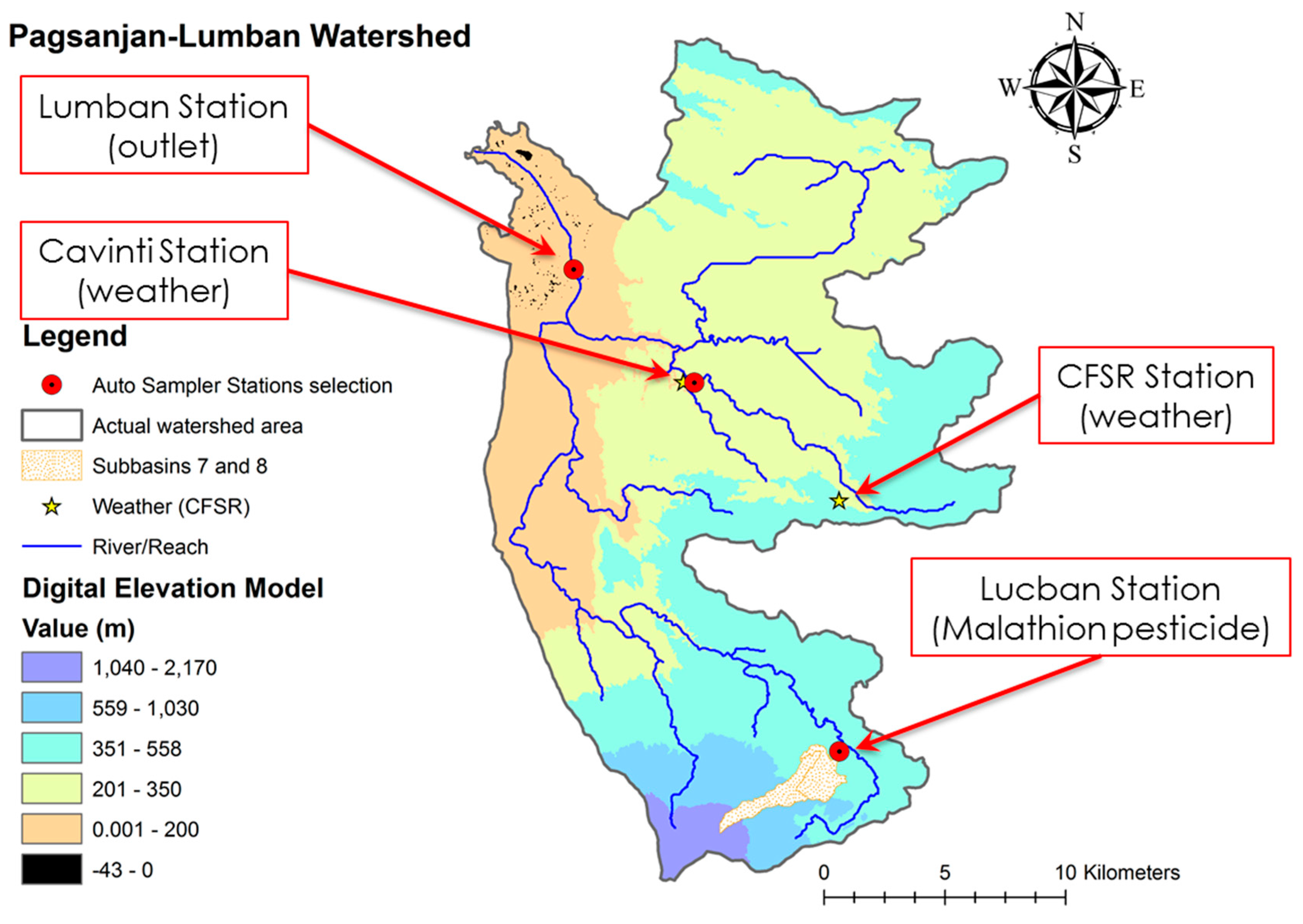
2.1. Study Area

PL basin is located at the southeastern part of Laguna de Bay basin in the Southern Tagalog Region (CALABARZON) of the Philippines. It has a catchment area of 454.45 km² (121°24′ E~121°37′ E, 14°37′ N~14°21′ N) that drains to Laguna de Bay. The watershed experiences two types of Philippine climate: (1) Type II; and (2) Type III. The eastern part of the basin experiences Type II climate that has no dry season with a very pronounced maximum rain period from December to February and a minimum rainfall period from March to May [28]. On the other hand, the western part has a Type III climate that has a short dry season, varying from 1 to 3 months, in December to February [28]. Areas close to Mt. Banahaw at the southernmost part of the basin have relatively uniform rainfall distribution throughout the year [29]. However, the basin in general experiences a dry period from November to April due to the rain shadow effect of the Sierra Madre mountain range while the wet period occurs for the remaining months [29]. The average annual rainfall of the basin is 2996 mm, which mostly fall during the monsoon period.

Figure 1 shows the Digital Elevation Model (DEM) of the PL basin. The areas near Mt. Banahaw at the southern region have the highest elevation, ranging from 560 m to 2170 m, while the eastern region near Sierra Madre ranges from 350 m to 560 m. The region near the outlet, including Lumban delta, has the lowest elevation, which ranges from 0 m to 200 m. Negative values can also be observed within the Lumban delta indicating that the elevations are below sea level and are often submerged in water. The outlet of the basin was set at the Lumban Station before the river branched out to the Lumban delta to exclude the possibility of water intrusion from the lake.

The basin has two major tributaries that branch out after the Lumban Station (outlet) as shown in Figure 1. Due to the presence of two reservoirs in the northern half of the basin, most of the discharge during dry days comes from the Pagsanjan River situated at the southern half of the PL basin. Pagsanjan River has a length of 54.1 km and a drainage area of 311.8 out of the 454.45 km² of PL basin, with a mean annual runoff of 53.1 m³·s⁻¹ [29]. The runoff pathways in the north were modified to collect the water in the reservoirs; hence, water only flows to the outlet during extreme rain events.

2.2. Monitoring Data

The locations of the monitoring stations for the flowrate, weather, and malathion are shown in Figure 1. The daily flowrate data from May 2014 to October 2016 at Lumban Station and the weather data (precipitation, temperature, humidity, and wind speed) at Cavinti Station from 2014 to 2016 were acquired from the Integrated National Watershed Research and Development Project (INWARD), the weather data from 1979 to 2014, including the solar values, were generated from the Climate Forecast System Reanalysis (CFSR) of the Global Weather Data for SWAT [30,31], and the malathion concentrations were monitored at Lucban Station by Varca [16]. A total of 26 sampling events at Lucban Station, with a frequency of at least two water samples a month, were carried out from December 2007 to November 2008 to measure the malathion concentrations. Each water sample was analyzed to measure the total concentration of malathion, which was used as comparison for the pesticide simulations in this study.

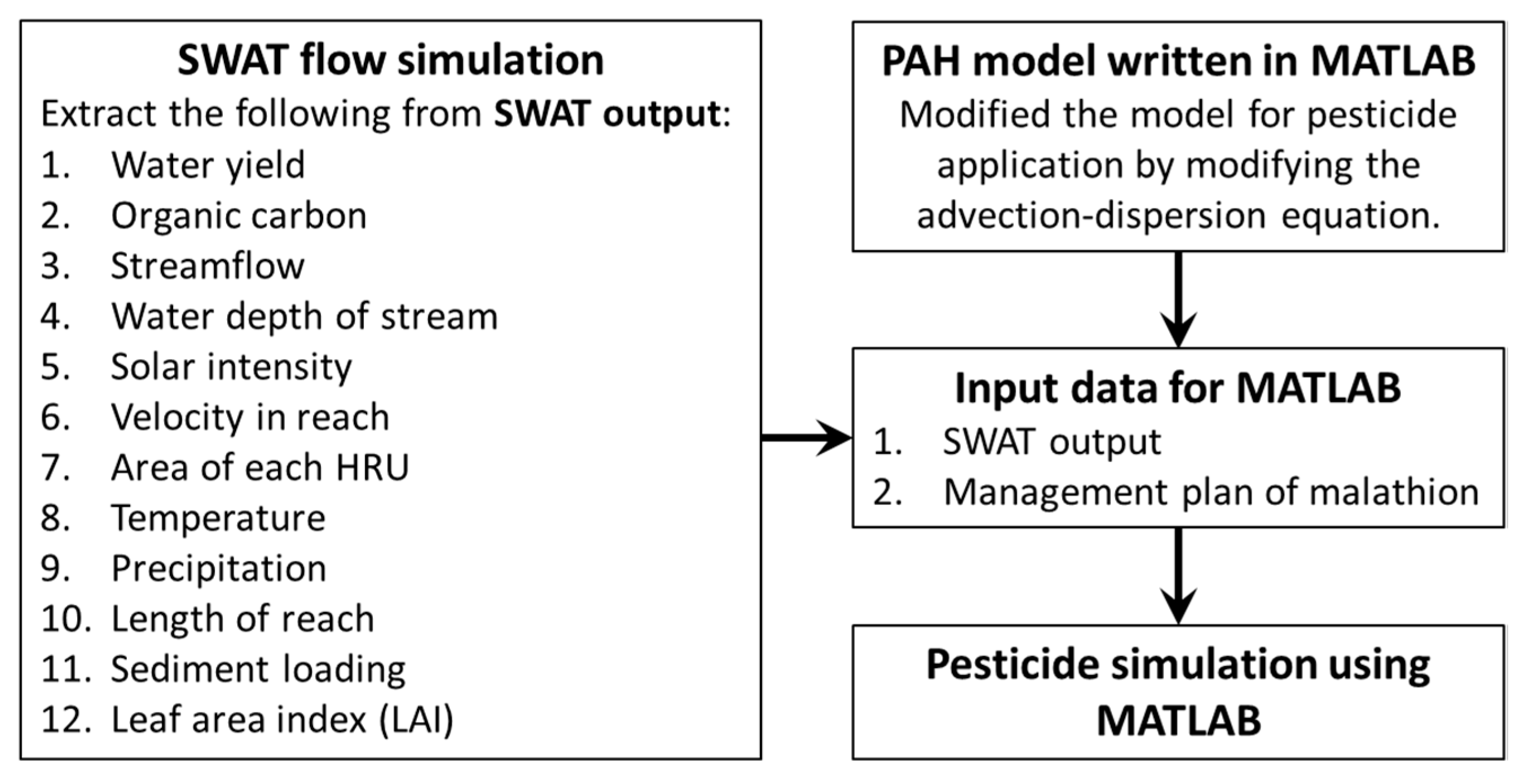
2.3. Hydrology Model

SWAT is a physically-based watershed model developed for the USDA Agricultural Research Service (ARS) to simulate the impact of land management practices on water, sediment, nutrients, and pesticide yields in large complex watersheds [32,33]. The model operates at a daily time step and uses readily available inputs such as [34]: topography (DEM with a 90 m resolution from United States Geological Survey (USGS)/National Aeronautics and Space Administration Shuttle Radar Topography Mission), hydrography, weather data (INWARD and CFSR), landuse/land cover (USGS Global Land Cover Characterization database), and soil type (Food and Agriculture Organization). The delineation threshold of the PL basin was 2.5 km², thus; it was divided into eight subbasins with 54 hydrological response units (HRU). Each of these HRUs is a unique combination of soil type, landuse, and slope. The threshold for soil, landuse, and slope was set to 0 to include non-agricultural areas in the basin that are less than 1% of the subbasin areas.

Table 1. Summary of the calibration and validation periods.

Process	Period
Spinup Time (2 years)	January 2005–December 2006
Pesticide Calibration	December 2007–November 2008
Flow Calibration	September 2014–May 2015
Flow Validation	May 2014–July 2014 and June 2016–September 2016

summarizes the calibration and validation periods of the flowrate simulation. The calibration period was from September 2014 to May 2015 while the validation was from May 2014 to July 2014 and June 2016 to September 2016. The available flowrate dataset started from May 2014 until September 2016. We first compared the observed flowrate to the precipitation and noticed that the peaks of the flowrate did not match the precipitation for a period. This period was removed after concluding that the sensor was faulty at that time. The SWAT—Calibration and Uncertainty Program (SWAT-CUP) was then used to calibrate and validate the SWAT flowrate parameters shown in

Table 2. Soil and Water Assessment Tool (SWAT) flowrate parameters for calibration and sensitivity analysis.

Parameter	Description	Module	Method	MIN	MAX
CN2	Initial SCS runoff curve number for moisture condition II	MGT	Relative	−0.1	0.1
BIOMIX	Biological mixing coefficiency	MGT	Replace	0	1
ALPHA_BF	Baseflow alpha factor (days)	GW	Replace	0.01	1
GW_DELAY	Groundwater delay time (days)	GW	Replace	0	500
GWQMN	Threshold depth of water in the shallow aquifer required for return flow to occur (mm H2O)	GW	Replace	0	50
REVAPMN	Threshold depth of water in the shallow aquifer for revap or percolation to the deep aquifer to occur (mm H2O)	GW	Replace	0	750
RCHRG_DP	Deep aquifer percolation fraction	GW	Replace	0.01	0.99
GW_REVAP	Groundwater “revap” coefficient	GW	Replace	0.02	0.2
ESCO	Soil evaporation compensation factor	HRU	Replace	0.7	1
EPCO	Plant uptake compensation factor	HRU	Replace	0.7	1
SLSUBBSN	Average slope length (m)	HRU	Replace	10	150
LAT_TTIME	Lateral flow travel time (days)	HRU	Replace	0	180
OV_N	Manning’s “n” value for overland flow	HRU	Replace	0.01	0.5
CANMX	Maximum canopy storage (mm H2O)	HRU	Replace	0	100
CH_K2	Effective hydraulic conductivity in main channel alluvium (mm/h)	RTE	Replace	0.025	76
CH_N2	Manning’s “n” value for the main channel	RTE	Replace	0.025	0.15
SOL_BD	Moist bulk density (Mg/m3 or g/cm3)	SOL	Relative	−0.1	0.1
SOL_CBN	Organic carbon content (% soil content)	SOL	Relative	−0.1	0.1
SOL_K	Saturated hydraulic conductivity (mm/h)	SOL	Relative	−0.1	0.1
SOL_AWC	Available water capacity of the soil layer (mm H2O/mm soil)	SOL	Relative	−0.1	0.1
CH_K1	Effective hydraulic conductivity in tributary channel alluvium (mm/h)	SUB	Replace	0.025	76
CH_N1	Manning’s “n” value for the tributary channel	SUB	Replace	0.025	0.15
SURLAG	Surface runoff lag coefficient (h)	BSN	Replace	0.05	10

. Simulated flowrates in 2007 and 2008 were then applied to simulate malathion fate based on the available malathion dataset (December 2007 to November 2008).

2.4. Pesticide Modeling

The malathion loadings were then calibrated using the original SWAT and modified SWAT pesticide models. Both models need the management operation schedule to simulate the application of pesticide in the basin. In this study, malathion was applied to HRUs with “Tomato” (TOMA) as land cover. This is based on a previous study that summarized the pesticide usage of the farmers in the PL basin, which affects two HRUs from Subbasins 7 and 8 (shown in Figure 1) [35]. TOMA was assumed as a collective representative of the vegetable crops in the PL basin that used malathion during the pesticide application period. Two planting seasons were implemented for TOMA. The first season starts in January while the second season starts in June. Malathion was then applied for 12 times for 3 months after planting at a rate of 0.57 kg/ha for every application (first season: January to March; second season: June to August). Based on this schedule, the pesticide models were then run to simulate malathion loading in the HRUs with TOMA as land cover. The models are further discussed in the next subsections.

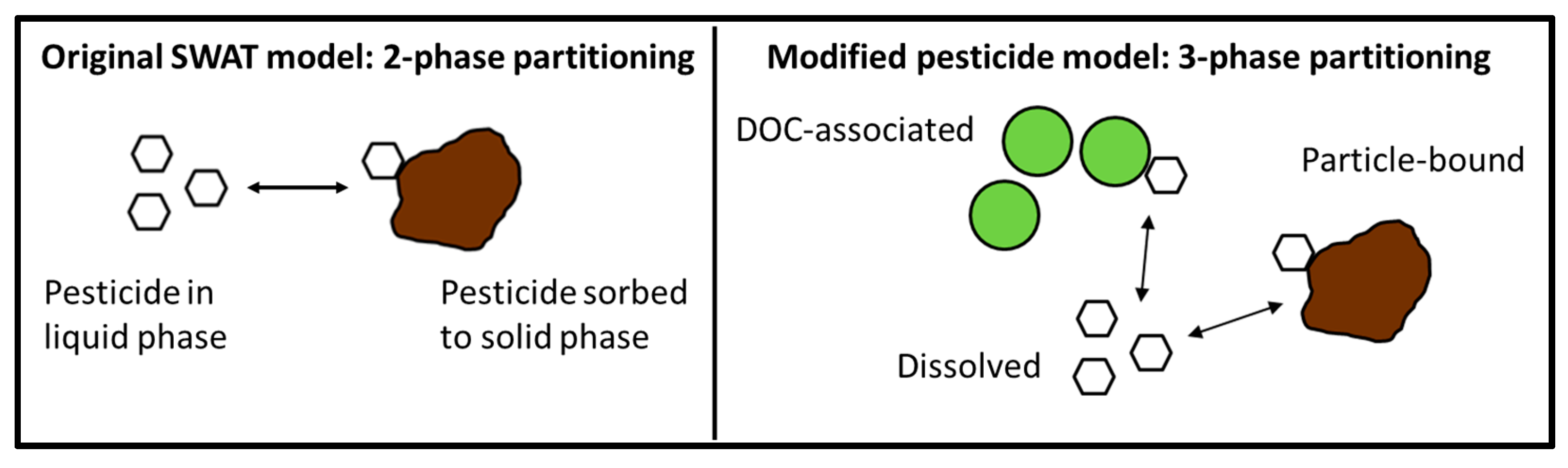
2.4.1. Original SWAT Pesticide Model

The pesticide module in the SWAT model was applied to calibrate the malathion loadings in the PL basin. Figure 2 shows that the SWAT pesticide model used the two-phase partitioning approach that classify the pesticides as: pesticide sorbed into solid phase and pesticide in solution or liquid phase.

Table 3. Pesticide parameters for calibration and sensitivity analysis of the original SWAT model.

Parameter	Description	Module	Method	MIN	MAX
SKOC	Soil adsorption coefficient normalized for soil organic carbon (L·kg−1)	PEST	Replace	1	5000
HLIFE_S	Degradation half-life of the chemical on the soil (day−1)	PEST	Replace	0	100
HLIFE_F	Degradation half-life of the chemical on the foliage (day−1)	PEST	Replace	0	100
WSOL	Solubility of the chemical in water	PEST	Replace	0	1000
WOF	Wash off fraction	PEST	Replace	0	1
AP_EF	Application efficiency	PEST	Replace	0	1
PST_DEP	Depth of pesticide incorporation in the soil (mm)	MGT	Replace	0	500
PERCOP	Pesticide percolation coefficient	BSN	Replace	0	1
CHPST_KOC	Pesticide partition coefficient between water and sediment in reach (m3·g−1)	SWQ	Replace	0	0.1
CHPST_REA	Pesticide reaction coefficient in reach (day−1)	SWQ	Replace	0	0.1
CHPST_VOL	Pesticide volatilization coefficient in reach (m·day−1)	SWQ	Replace	0	10
CHPST_STL	Settling velocity for pesticide sorbed to sediment (m·day−1)	SWQ	Replace	0	10
SEDPST_REA	Pesticide reaction coefficient in reach bed sediment (day−1)	SWQ	Replace	0	0.1
CHPST_RSP	Resuspension velocity for pesticide sorbed to sediment (m·day−1)	SWQ	Replace	0	1
SEDPST_ACT	Depth of active sediment layer for pesticide (m)	SWQ	Replace	0	1
CHPST_MIX	Mixing velocity (diffusion/dispersion) for pesticide in reach (m·day−1)	SWQ	Replace	0	0.1
SEDPST_BRY	Pesticide burial velocity in reach bed sediment (m·day−1)	SWQ	Replace	0	0.1
PSTENR	Enrichment ratio for pesticide in the soil	CHM	Replace	0	5

shows the pesticide parameters that describe the reaction and transport processes of malathion starting from the application (foliar, soil surface, and subsurface). These processes include degradation, infiltration, leaching, surface runoff, volatilization, and wash off mechanisms.

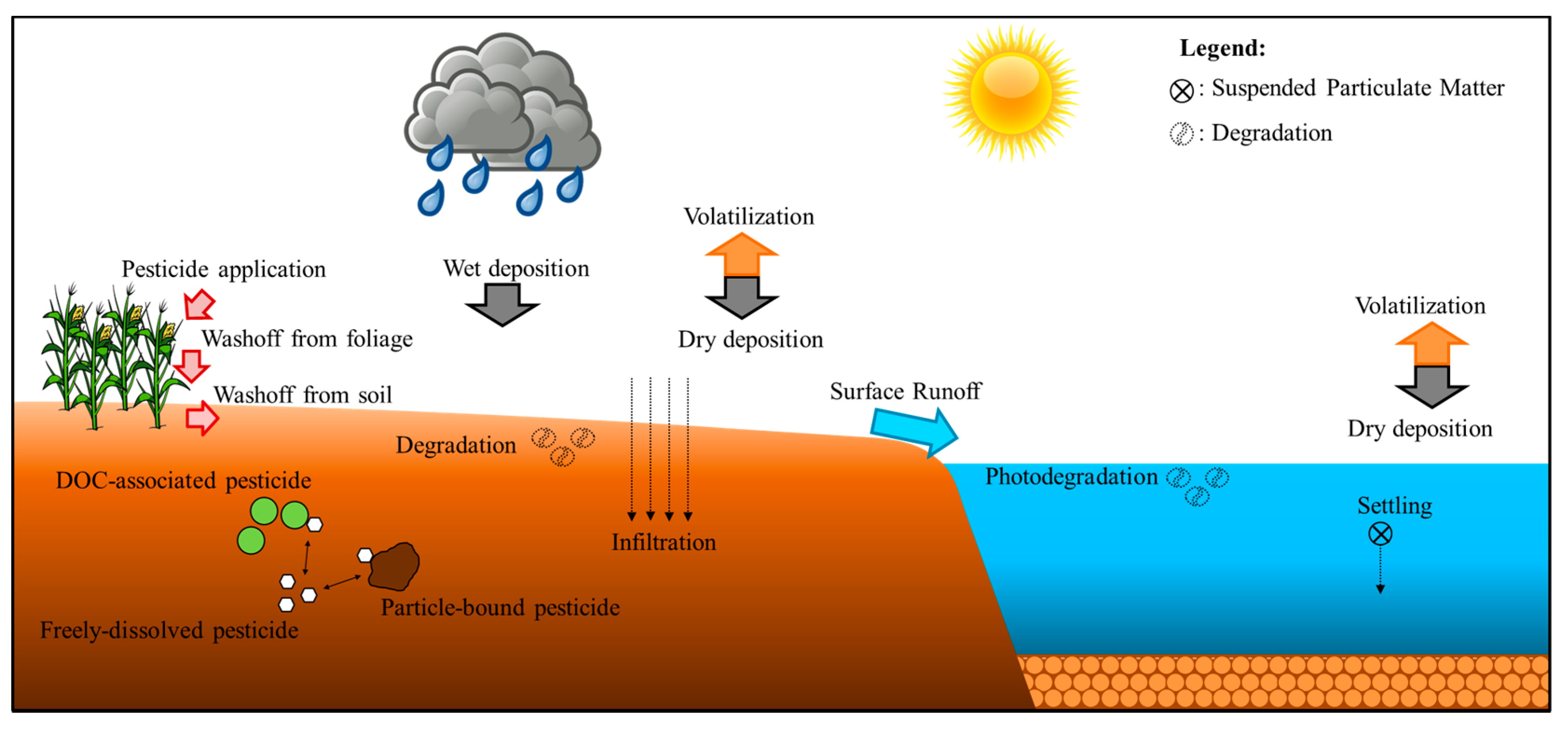
2.4.2. Modified Pesticide Model

Figure 3 shows the schematic diagram of the fate and transport of the pesticides for the modified SWAT pesticide model. The modified model applied in this study was based on the watershed-scale model from a previous study of the same authors about modeling the fate and transport of polycyclic aromatic hydrocarbons (PAH) and linking the PAH model with SWAT [36]. This study further developed the model to include the pesticide application based on the original SWAT model and other equations related to the fate and transport of pesticides. The approach of the original 2-phase partitioning SWAT model on the fate and transport of pesticides was modified by considering the three-phase partitioning model shown in Figure 2. Figure 4 shows the diagram of using MATLAB as platform for the modified approach.

Table 4. Pesticide parameters for calibration and sensitivity analysis of the modified model.

Parameter	Description	Unit
foc	Organic carbon fraction in soil	-
ρsoil	Soil density	kg·m−3
poro	Porosity
fDOC	Fraction of the dissolve organic carbon	-
x1	Enrichment ratio coefficient 1	-
x2	Enrichment ratio coefficient 2	-
vs	Settling velocity of suspended particles in the channel	m·s−1
En	Diffusion coefficient	-
Cp,1	Wash off coefficient for particle-bound pesticide	-
Cfd,1	Wash off coefficient for dissolved pesticide	-
Cp,2	Wash off exponent for particle-bound pesticide	-
Cfd,2	Wash off exponent for dissolved pesticide	-
α	Decay coefficient in water due to solar intensity	-
CDOC,1	Wash off coefficient for DOC-associated pesticide	-
CDOC,2	Wash off exponent for DOC-associated pesticide	-
µk,p	Degradation rate constant for the particle-bound pesticide on the soil surface	s−1
θk,p	Temperature adjustment factor for particle-bound pesticide	-
µk,fd	Degradation rate constant for the dissolved pesticide on the soil surface	s−1
θk,fd	Temperature adjustment factor for dissolved pesticide	-
µk,DOC	Degradation rate constant for the DOC-associated pesticide on the soil surface	s−1
θk,DOC	Temperature adjustment factor for DOC-associated pesticide	-

shows the parameters of the modified pesticide model.

Accumulation of Pesticide

Pesticides are usually distributed to the foliage and soil surface during application. In this case, separate equations were applied to calculate the amount of pesticides on the foliage and the soil surface [37]. This approach is similar to the original SWAT model. The amount of pesticides on foliage (pst_f, kg of pesticide ha⁻¹) and on the soil surface (pst_surf, kg of pesticide ha⁻¹) were determined by the equations below [37]:

pst_f = gc × pst′

(1)

pst_surf = (1 − gc) × pst′

(2)

where gc is the fraction of the ground surface covered by plants (-) and pst′ is the efficient amount of pesticide applied (kg of pesticide ha⁻¹). These terms were determined by the following equations [37]:

gc = (1.99532 − erfc × [1.333 × LAI − 2])/2.1

(3)

pst′ = ap_ef × pst

(4)

where erfc is the complementary error function (-), LAI is the leaf area index (-), ap_ef is the pesticide application efficiency (-), and pst is the original amount of pesticide applied (kg of pesticide ha⁻¹).

Pesticide on the foliage was assumed to be affected by wash off due to rain events and degradation. The amount of pesticides washed off by precipitation from the plants (pst_f,wsh, kg of pesticide ha⁻¹) were determined using the equation below [37]:

pst_f,wsh = fr_wsh × pst_f

(5)

where fr_wsh is the wash off fraction for the pesticide on the foliage (-). Degradation of pesticide on the foliage was then calculated using the following equation [37]:

pst_f,t = pst_f,0 × exp[-k_p,f × t]

(6)

where pst_f,t is the amount of pesticide on the foliage at time t (kg of pesticide ha⁻¹), pst_f,0 is the initial amount of pesticide on the foliage (kg of pesticide ha⁻¹), k_p,f is the degradation rate constant of the pesticide (day⁻¹), and t is time (day).

Pesticides on Soil

The original SWAT model assumed that the pesticide is either sorbed to the solid phase or dissolved in solution [37]. The three-phase partitioning model was used to estimate the different forms of pesticide in the soil. This method classifies the pesticide into three classes: dissolved pesticide, pesticide adsorbed on dissolved organic carbon ([DOC]), and pesticide adsorbed on particles. The total pesticide and dissolved pesticide concentrations in the bulk saturated soil are defined by the following equations [38]:

C_bs^t = C_bs^p + C_bs^d

(7)

C_bs^d = C_bs^fd + C_bs^D°^C

(8)

where C_bs^t is the total pesticide concentration in the bulk soil (kg·L⁻¹ bulk soil), C_bs^p is the concentration of particle-bound pesticide (kg·L⁻¹ bulk soil), C_bs^d is the dissolved pesticide concentrations in the bulk saturated soil (kg·L⁻¹ bulk soil), C_bs^fd is the dissolved pesticide, and C_bs^DOC is the DOC-associated pesticide. Combining Equations (7) and (8) yields the following equation:

C_bs^t = C_bs^p + C_bs^fd + C_bs^D°^C

(9)

The terms C_bs^p and C_bs^D°^C can also be determined by multiplying C_bs^fd by the coefficients shown in Equations (10)–(12) below [38]:

C_bs^p = r_sw × K_sw × C_bs^fd

(10)

C_bs^D°^C = [DOC] × K_DOC × C_bs^fd

(11)

[DOC] = f_DOC × OM

(12)

where r_sw is the soil-to-water ratio (kg·L⁻¹), K_sw is the soil-water distribution coefficient [L·kg⁻¹], K_DOC is the dissolved organic carbon-water partition coefficient (L·kg⁻¹), f_DOC is the fraction of DOC, and OM is the concentration of the organic matter (kg·L⁻¹). OM was calculated by dividing the mass of the soil carbon in the soil organic matter with the water yield, which were both simulated by the original SWAT model [36]. C_bs^p, C_bs^fd, and C_bs^D°^C from Equation (9) can also be determined by using the pesticide in bulk soil fractions [36,38]:

C_bs^p = f_p × W_cp × exp(-μ_p) × ε_pstsed

(13)

C_bs^fd = f_d^fd × W_cf × exp(-μ_f)

(14)

C_bs^D°^C = f_d^D°^C × W_cDOC × exp(-μ_DOC)

(15)

where f_p (-), W_cp (kg·L⁻¹ bulk soil), and μ_p (s⁻¹) are the fraction, wash off load, and rate constant of particle-bound pesticide, ε_pstsed is the enrichment ratio (-), f_d^fd (-), Wcf (kg·L⁻¹ bulk soil), and μ_f (s⁻¹) are the fraction, wash off load, and rate constant of dissolved pesticide, and f_d^DOC (-), W_cf (kg·L⁻¹ bulk soil), and μ_DOC (s⁻¹) are the fraction, wash off load, and rate constant of DOC-bound pesticide. The enrichment ratio was calculated using this equation [37]:

ε_pstsed = x₁ × (sed/WY)^x₂

(16)

where x₁ and x₂ are the enrichment ratio coefficients, sed is the sediment yield (metric tons), and WY is the water yield (mm H₂O). Surface runoff of the suspended particles to the channel was also considered in the wash off loads and wash off fractions of the pesticide. The suspended particles affected by the wash off mechanism are described in the following equations [36]:

W_cp = C_p1 × q^C_p2 × C_bs^t

(17)

W_cf = C_f1 × q^C_f2 × C_bs^t

(18)

W_cDOC = C_DOC1 × q^C_DOC2 × C_bs^t

(19)

where W_cp, W_cf, and W_cDOC are the wash off loads of the particle-bound, dissolved, and DOC-associated PAHs exported to the river via runoff (kg·L⁻¹ bulk soil); C_p1, C_f1, and C_DOC1 are the wash off coefficients for the particle-bound, dissolved, and DOC-associated PAHs (-); q is the runoff rate per unit area; and C_p2, C_f2, and C_DOC2 are the wash off exponents for the particle-bound, dissolved, and DOC-associated PAHs (-), respectively.

The degradation term, previously shown in Equations (13)–(15), is a temperature-dependent rate constant expressed as the first-order reaction. The rate constant for the three phases was defined as:

μ = μ_i × θ^{(T − 2}°⁾

(20)

where μ_i is the initial rate constant for the pesticide [s⁻¹], θ is the temperature adjustment factor for pesticide (-), and T is the temperature (°C). μ and θ were then calibrated for the particle-bound, dissolved, and DOC-associated pesticide.

Pesticide loadings on the soil and into the water were computed by [38]:

C_p = (C_bs^p − C_bs,out^p)/ρ

(21)

C_wfinal = C_bs^d + C_bs,out ^p

(22)

where C_p and C_w are the pesticide loading on soil [pesticide per solid mass] and in water [pesticide per fluid mass], respectively, and C_wfinal is the final pesticide loading in water.

Pesticides in Water

The pesticides in the channels are then subjected to the following mechanisms and processes due to water movement and reactivity of the pesticide with other components present in the water: advection, dispersion, photodegradation, and settling processes upon entering the channel [36]. The concentration of the pesticide in the waterbody was determined after considering these processes. This is expressed by the modified advection-dispersion equation:

(∂C/∂t) + u × (∂C/∂x) = D_L × (∂²C/∂x²) − C × [f × (v_s/h) + aI]

(23)

where C is the concentration of pesticide in water (g·m⁻³), t is time (day), x is distance (m), u is the velocity of the water (m·s⁻¹), D_L is the dispersion coefficient (m²·d⁻¹), f is the fraction of the particulate pesticide in water (-), v_s is the settling velocity (m·s⁻¹), h is the depth of the channel (m), a is the photodegradation coefficient (m²·MJ⁻¹·d⁻¹), and I is the solar intensity (MJ·m⁻²). The photodegradation term in the equation was added to the advection-dispersion equation to fit the pesticide model.

2.5. Sensitivity Analyses

The sensitivity analyses for the flowrate and pesticide were simultaneously done with the calibration. SWAT-CUP applies the Latin-Hypercube (LH) sampling method, which is based on the Monte Carlo simulation, and set the Nash–Sutcliffe efficiency (NSE) as the objective function (Section 2.6). This is a robust method that requires a large number of simulations and computational resources [39]. LH sampling randomly assigns a value within the permitted range of each parameter to complete a parameter set. The One-factor-At-a-Time (OAT) sensitivity test was then commenced after the sampling. This method takes one parameter for each run and changes its value to determine how each parameter affects the results. Sensitive parameters were determined based on their probability values or p-values. Parameters with less than 0.01 p-value were labeled as sensitive. The LH-OAT method was applied to the SWAT hydrology and pesticide models in this study.

2.6. Evaluation Criteria

The coefficient of determination (R²), Nash–Sutcliffe Efficiency coefficient (NSE), root mean square error (RMSE), and percent bias (PBIAS) were then calculated to evaluate the SWAT and the modified model. These statistical indices can determine whether the model performance is satisfactory or unsatisfactory [40]. R² and NSE were calculated for the calibration and validation periods of the flowrate (Table 1), while R², NSE, RMSE and PBIAS were determined for pesticide. For a daily time-step, the model is acceptable or satisfactory when the R² and NSE values are greater than 0.5 and when the RMSE and PBIAS values reach the optimal value of 0. A lower RMSE value is an indicator that the model has less residual variance [41]. PBIAS shows if the model has under- or overestimated the results compared to the observations, and lower absolute PBIAS values indicate more accurate model simulations [42].

SWAT-CUP also has other criteria to quantify the strength and uncertainties of the calibration analysis. Given the small dataset of this study, the P-factor and R-factor of the iteration were also noted. P-factor represents percentage of the simulated data covered by the 95% uncertainty band (95PPU) and it ranges from 0 to 1 [43]. A P-factor value greater than 0.5 is desirable since it entails that more than 50% of the simulated data are acceptable. R-factor, on the other hand, estimates strength of the calibration by dividing the average thickness of the 95PPU band with the standard deviation of the measured data [43]. The range of the R-factor starts from 0 to infinity; high and low R-factor values correspond to a thicker and thinner 95 PPU bands, respectively. A P-factor of 1.0 and an R-factor of 0 signifies a perfect simulation of the observed data.

3. Results and Discussion

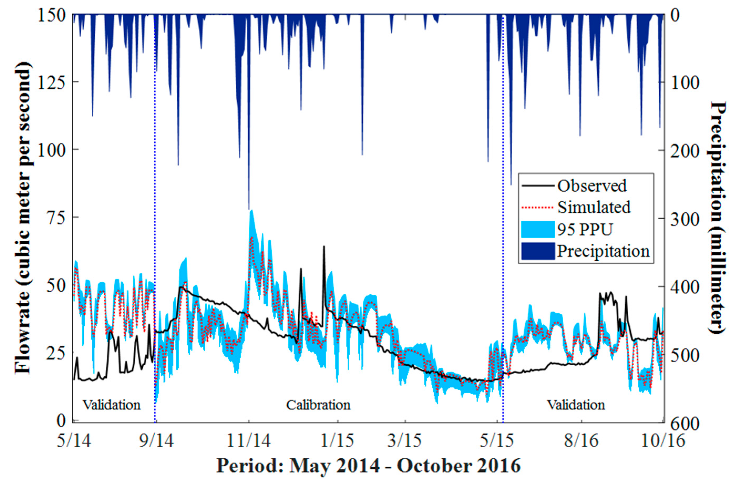
3.1. Flowrate Calibration

Figure 5 shows the comparison of the observed and SWAT-simulated flowrate at Lumban Station. The model did not implement the presence of reservoirs and paddy fields due to the lack of information; hence, it was assumed that these factors would affect the flowrate calibration when it comes to water storage. The calibration process yielded an R² value of 0.42 and an NSE of 0.22 while the validation period has 0.10 and −2.87, respectively. These values are less than the desired value of 0.5 [40], showing that the SWAT model is slightly unfit and underperforming. The lack of information regarding the management of the two reservoirs (storage, release, and distribution) may have significantly degraded the performance of the model [44]. The SWAT model of the PL basin was limited to a small dataset, which was a major disadvantage during the calibration (227 observed flowrate) and validation (158 observed flowrate) of the flowrate. The intense rainfall events happened in the calibration period; hence, the entire basin drains to the outlet, as mentioned in Section 2.1. This is in contrast with the validation period that included the days with dry to mild rainfall, which only drains the southern part of the basin. The 95PPU band of the flowrate calibration in Figure 5 has a P-factor value greater than 0.5 and an R-factor value of less than 1. This result indicates that more than 50% of the simulated flowrate is within the acceptable uncertainty [43]. The validation period, on the other hand, has a P-factor of 0.18 and an R-factor of 0.72, indicating that only 18% of the simulated flowrate during this period is within the uncertainty range.

Nine parameters were found to have a significant effect on the flowrate (

Table 5. SWAT parameters for calibration and sensitivity analysis of the original SWAT pesticide model.

Rank	Parameter	Fitted Value
1	SURLAG	0.051
2	CH_N1	0.12
3	CN2	−0.096
4	ALPHA_BF	0.46
5	CH_K1	48.4
6	RCHRG_DP	0.97
7	CH_K2	42.2
8	SLSUBBSN	75.8
9	OV_N	0.33

). Surface runoff lag coefficient (SURLAG) was the most sensitive parameter with a calibration value of 0.051 h. This value is negligible compared to the default value in SWAT, which is four hours. As SURLAG decreases, more water is stored in the basin, indicating that surface runoff does not go directly to the channel in the PL basin and is instead stored elsewhere [45]. The presence of two reservoirs in the northern half of the basin, mentioned in Section 2.1, may have affected the SURLAG value. A huge percentage of the runoff was immediately collected by the reservoirs instead of getting released across the basin. The water can also be stored in the foliage and paddies that are present in the basin. This is supported by the other sensitive parameters: Manning’s “n” value for the tributary channels (CH_N1), second most sensitive; the initial SCS runoff curve number for moisture condition II (CN2), third; baseflow alpha factor (ALPHA_BF), fourth; and effective hydraulic conductivity in tributary channel alluvium (CH_K1), fifth.

CN2 signifies the soil permeability of the basin [46]. Increasing CN2 values is associated with the increase of imperviousness of the basin. This can be related to how urbanized the basin is. During calibration, SWAT-CUP relatively changes the CN2 value at the HRU level since HRUs have varying CN2 values. In general, CN2 in PL basin has a calibrated value of −0.096 or −9.6%, indicating a general decrease in the CN2 values of each HRU. Hence, the basin is slightly more pervious compared to the default values suggested by SWAT. This result was expected since PL basin is highly agricultural [29]. ALPHA_BF, on the other hand, is the baseflow recession constant, a direct index of groundwater flow response and is a basin-wide parameter. It has a calibrated value of 0.46, suggesting an intermediate or average response to the change in recharge, slightly leaning towards the slow response (slow response: 0.1–0.3; rapid response: 0.9–1.0). The result can indicate that it is possible for water to be stored in the shallow aquifer that can also be associated to the CH_K1 value. CH_K1 controls the transmission losses from the surface runoff in the tributary. It is determined by the type of bed materials present in the channel bed. The calibrated result of 48.4 mm·h⁻¹ falls on the moderately high loss rate that ranges from 25 mm·h⁻¹ to 76 mm·h⁻¹. This value characterizes the tributary bed material as sand and gravel mixture with low silt-clay content, which makes it easier for the transmission losses of to percolate into the shallow aquifer. Another sensitive parameter that has a similar description to CH_K1 is the effective hydraulic conductivity in the main channel alluvium (CH_K2). The calibrated value of CH_K2, 42.2 mm·h⁻¹, falls within the same range as CH_K1, indicating that the main channel has similar characteristics as the tributary channel. Having a lower CH_K2 value compared to CH_K1 signifies that the bed material of the main channel is a slightly more consolidated compared to the tributary channels. The second most sensitive parameter also describes the tributary channel in the basin, CH_N1. CH_N1 has a calibrated value of 0.12, which indicates the channel is well maintained and full of weeds and brushes (excavated or dredged) or it is heavy timbered with lots of vegetation as well (natural stream). The deep aquifer percolation fraction (RCHRG_DP) was also found to be sensitive, with a calibrated value of 0.97. This result indicates that a huge fraction of percolation from the root zone recharges the deep aquifer [47]. However, the value is extremely high compared to the other studies with high RCHRG_DP values. Schuol et al. [48] estimated a range of 0.4 to 0.65 for the West Africa subcontinent, while Me et al. [47] yielded a value of 0.87 for a New Zealand catchment with mixed landuse. Though it can be assumed that the RCHRG_DP value for PL basin is also high, it should also be noted that this parameter may have been affected by the discrepancies formulated from the limited dataset (Section 2.2) and that the fraction (0.97) is too high for this basin. Lastly, the average slope length (SLSUBBSN) and Manning’s value for overland flow (OV_N) have calibrated values of 75.8 m and 0.33, respectively.

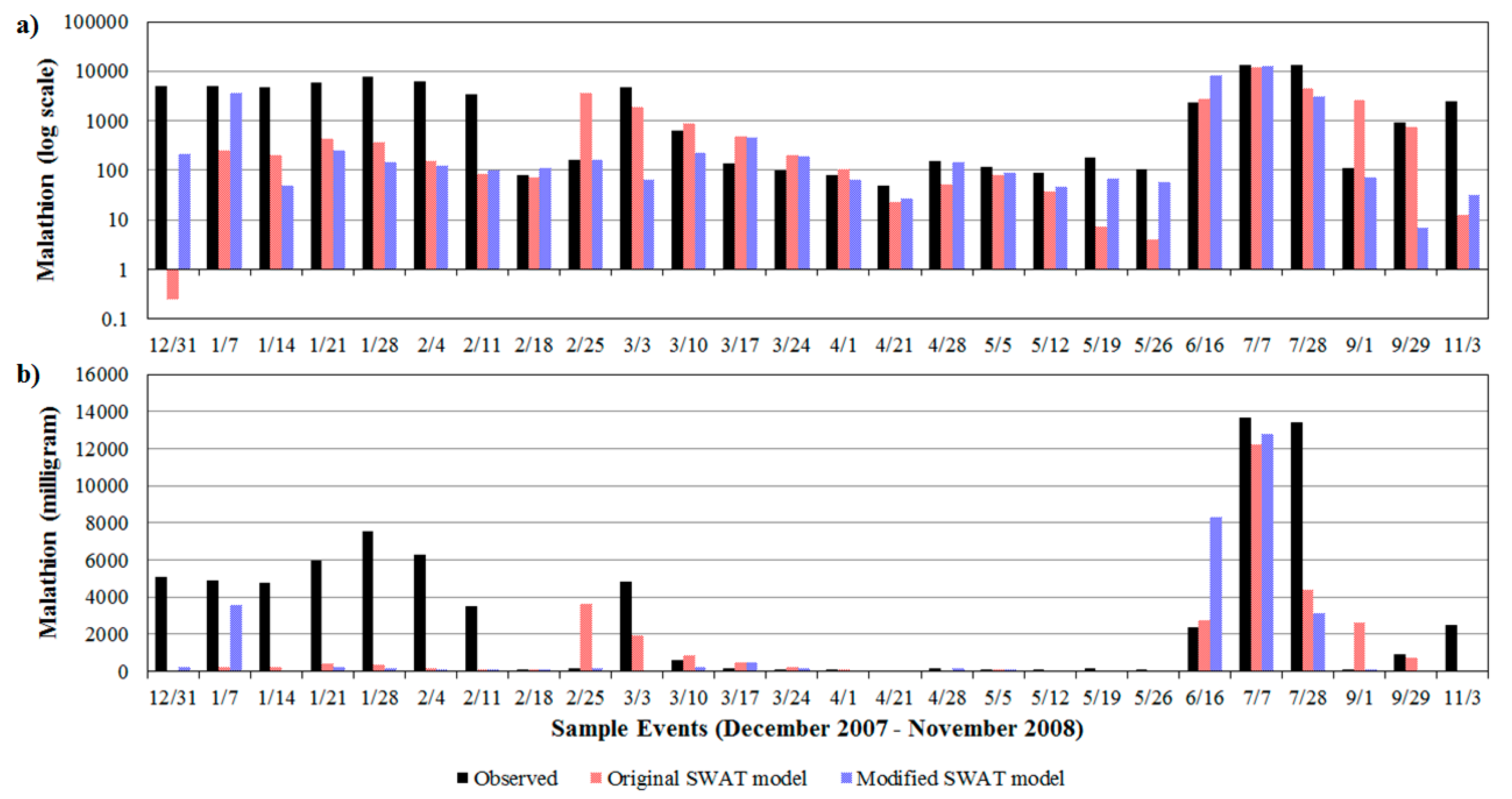
3.2. Pesticide Calibration with SWAT Pesticide Model

After the flow calibration and validation, SWAT-CUP was applied to calibrate and analyze the sensitive parameters of the SWAT pesticide model. The calibration processes of the flowrate and pesticide were done separately to incorporate the same calibrated values of the flowrate parameters for the original SWAT model and the modified model. Figure 6 shows the observed and the simulated results of the malathion concentrations at Lucban Station using the original SWAT model. The calibration process yielded an R² of 0.39, an NSE of 0.18, a PBIAS value of 59.2%, and an RMSE of 3492.23 mg. Five parameters were found to be significant in the SWAT pesticide model (

Table 6. Sensitive parameters of the SWAT pesticide model.

Rank	Parameters	Fitted Value
1	AP_EF	0.13
2	CHPST_KOC	0.0012
3	HLIFE_S	6.26
4	CHPST_REA	0.037
5	SKOC	3594.52

). The most sensitive parameter was the application efficiency (AP_EF) of the malathion with a calibrated value of 0.13. This indicates that only 13% of the applied malathion is deposited on the foliage and soil surface while the rest are lost in the atmosphere, which can be due to the type of pesticide application and management practices of the farmers in the basin. The pesticide partition coefficient between water and sediment in the reach (CHPST_KOC) was the second most sensitive parameter with a fitted value of 0.0012. A low value indicates that malathion is highly mobile in the water in its dissolved form, thereby increasing its potential for long-distance transport [16,49]. This parameter is followed by the degradation half-life of malathion on the soil surface (HLIFE_S), the reaction coefficient in the channel (CHPST_REA), and the soil adsorption coefficient for soil organic carbon (SKOC) that have calibrated values of 6.26 day⁻¹, 0.037 day⁻¹, and 3594.52 L·kg⁻¹, respectively. The sensitivity analysis determined that the pesticide application, degradation in the soil, and the sediment interaction and reactivity of malathion in water were the important processes that influenced the fate and transport of malathion in the basin.

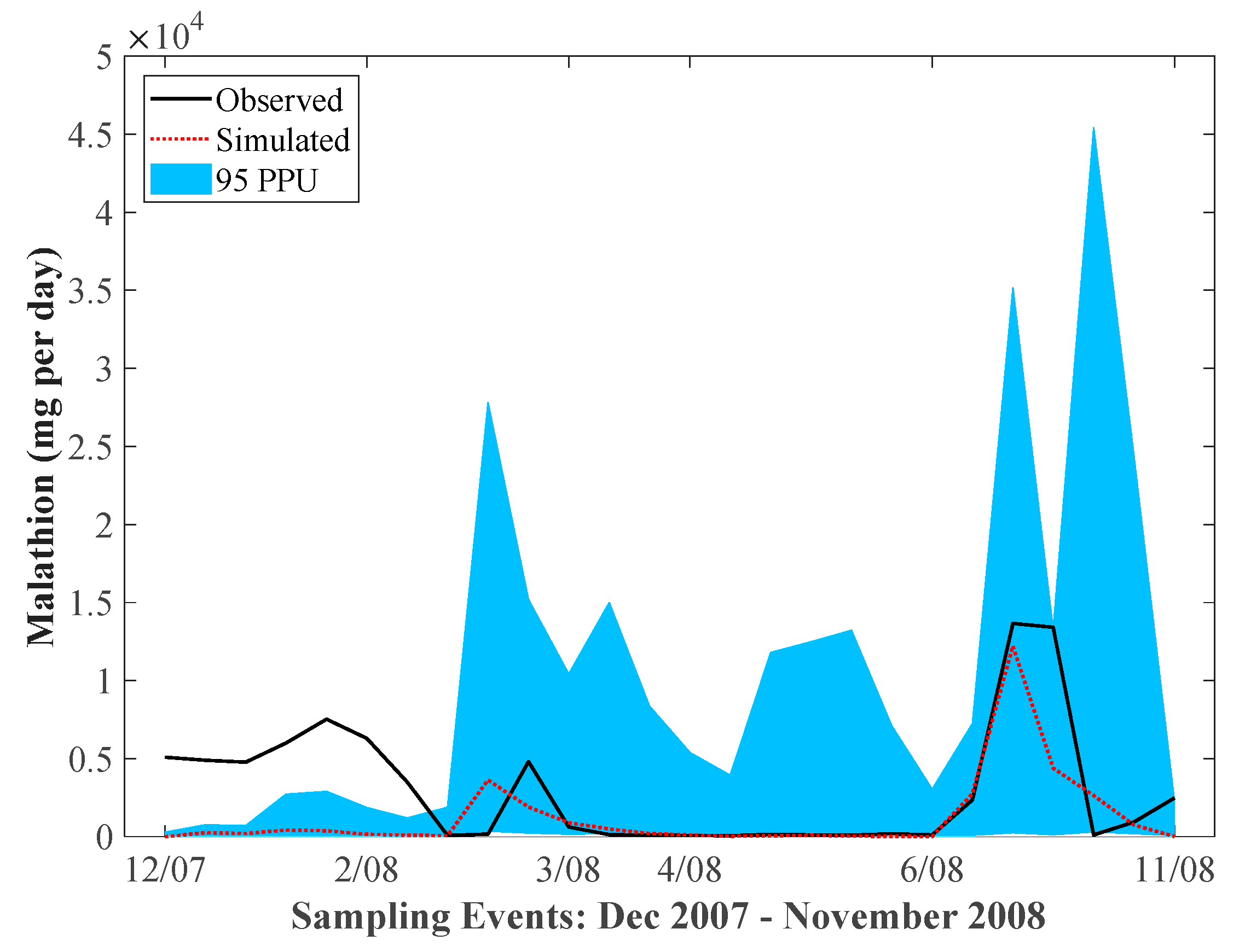
3.3. Pesticides Calibration with Modified Pesticide Model

Table 7. Sensitive parameters of the modified pesticide model.

Rank	Parameters	Fitted Value
1	vs	0.0001
2	µk,fd	4.25 × 10−5
3	Cfd,1	1.14
4	Cfd,2	0.549
5	poro	0.50
6	foc	0.20
7	En	0.1006
8	θk,p	1.16 × 10−5
9	ρsoil	1.06

revealed that the settling velocity (v_s) was the most sensitive parameter, which suggest that the interaction of malathion particles in the water greatly affects the malathion transport. Degradation rate constant of the dissolved malathion particles (µ_k,fd) was the second most sensitive, which can be attributed to how malathion readily dissolves in water compared to soil. This was followed by, in no particular order, the wash off coefficient (C_fd,1) and exponent (C_fd,2), diffusion coefficient (En), porosity (poro), soil density (ρ_soil), organic carbon fraction in soil (f_oc), and temperature adjustment factor of the particle-bound malathion (θ_k,p). Malathion parameters that are associated with the particulate phase were sensitive for both models. However, the specific parameters are not exactly the same. The modified model has a more detailed formalism since it applied the three-phase partitioning model. This gave a visual understanding of the different forms of malathion that were greatly affected by wash off, which is the dissolved malathion. In this case, it can be assumed that dissolved malathion is more susceptible to wash off and most likely to end up in the channel compared to the other two malathion phases, particle-bound and DOC-associated malathion. Aside from the malathion-specific parameters, soil properties were also important such as the soil density, porosity, and organic carbon fraction of the soil.

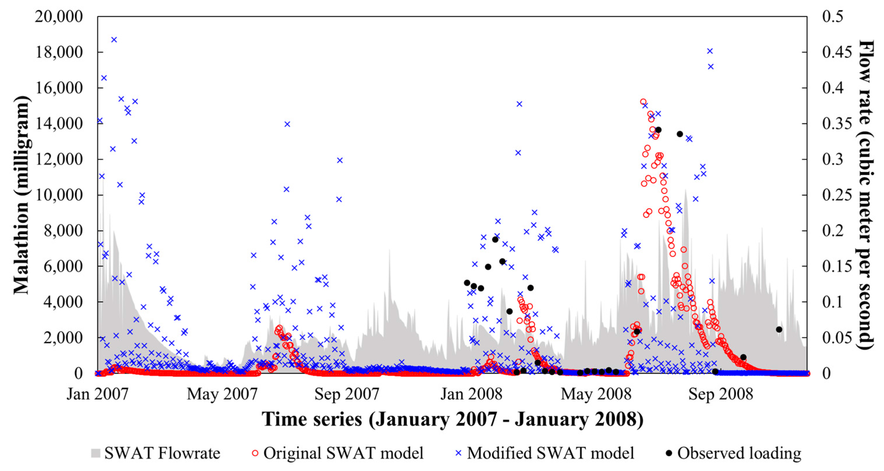
3.4. Comparison of Observed and Simulated Malathion Loading

Figure 7 shows the observed and simulated values of the monitoring dataset. The modified model has 0.52, 0.36, 48.6%, and 3088.05 mg values for R², NSE, PBIAS, and RMSE, respectively. Based on these evaluation criteria, the modified model performed better compared to the SWAT model (statistics mentioned in Section 3.2).

The observed data were compared to the simulated loading by SWAT and the modified model in Figure 8. The figure includes the logarithmic (Figure 8a) and actual (Figure 8b) scale of the values, which reveals the similarities and differences between the models. Both models were able to achieve a small deviation between the observed and simulated low malathion loading. Comparing the two simulations, the modified model captured more low values compared to SWAT. However, the models were poorly able to simulate the high values as seen in the two plots (Figure 7), the results were comparable for both models. Figure 7 shows the time series of the malathion loading simulated by the SWAT and modified models compared to the SWAT-projected flowrate from January 2007 to December 2008 at the Lucban Station. The malathion simulations peaked during the duration of the pesticide application. However, the peaks of modified model showed more consistency compared to the increasing peaks of the SWAT model. Both models have similar peak levels at the fourth peak, but the SWAT model gave a more distinct pattern compared to the modified model.

4. Conclusions

Insufficient data were one of the limitations of this study that imply high uncertainty in both models. However, building a SWAT model for the flowrate calibration was made possible in this study. Equations that are relevant to the fate and transport of pesticides were added to the modified model prior to simulations. The objectives of this study were also met by simulating the malathion loading in the PL basin using the SWAT and modified model. Hence, the following conclusions were derived:

• The sensitivity analysis of the hydrology model revealed that the flowrate of the PL basin is greatly influenced by the perviousness of the soil and the characteristics of the tributary channel that stores and retains the water in the basin.
• The modified pesticide model gave a slightly better performance compared to the original SWAT model, considering the statistical analyses performed (R², NSE, PBIAS, and RMSE).
• Application efficiency was the most sensitive parameters for the original SWAT model, suggesting a possible need to improve the pesticide application and management practices of farmers in the basin, while settling velocity was the most sensitive for the modified models. Parameters associated with particulate-phase malathion, especially the degradation of particle-bound malathion, were also significant to both models.
• The temporal patterns of the target subbasin simulated by the models showed that the modified model has more consistent peaks during the duration of pesticide application compared to SWAT.

This study focused on the comparison of the outcomes of the modified model with the commonly used SWAT hydrological model. The modified model and the original SWAT model were able to identify similar sensitive parameters. However, further development of the model is needed to incorporate pesticide application scenarios and interaction of soil and water media to the atmosphere.

References

1. The World Bank. Agriculture, Value Added (% of GDP). In World Development Indicators, 17 November 2016 ed.; The World Bank Group: Washington, DC, USA, 2016. [Google Scholar]
2. Bassil, K.L.; Vakil, C.; Sanborn, M.; Cole, D.C.; Kaur, J.S.; Kerr, K.J. Cancer health effects of pesticides: Systematic review. Can. Fam. Phys. 2007, 53, 1704–1711. [Google Scholar]
3. Colborn, T.; vom Saal, F.S.; Soto, A.M. Developmental effects of endocrine-disrupting chemicals in wildlife and humans. Environ. Health Perspect. 1993, 101, 378–384. [Google Scholar] [CrossRef] [PubMed]
4. Bolognesi, C. Genotoxicity of pesticides: A review of human biomonitoring studies. Mutat. Res. 2003, 543, 251–272. [Google Scholar] [CrossRef]
5. Jacobsen, C.S.; Hjelmsø, M.H. Agricultural soils, pesticides and microbial diversity. Curr. Opin. Biotechnol. 2014, 27, 15–20. [Google Scholar] [CrossRef] [PubMed]
6. Geiger, F.; Bengtsson, J.; Berendse, F.; Weisser, W.W.; Emmerson, M.; Morales, M.B.; Ceryngier, P.; Liira, J.; Tscharntke, T.; Winqvist, C.; et al. Persistent negative effects of pesticides on biodiversity and biological control potential on european farmland. Basic Appl. Ecol. 2010, 11, 97–105. [Google Scholar] [CrossRef]
7. Schäfer, R.B.; Caquet, T.; Siimes, K.; Mueller, R.; Lagadic, L.; Liess, M. Effects of pesticides on community structure and ecosystem functions in agricultural streams of three biogeographical regions in Europe. Sci. Total Environ. 2007, 382, 272–285. [Google Scholar] [CrossRef] [PubMed]
8. Wauchope, R. The pesticide content of surface water draining from agricultural fields—A review. J. Environ. Qual. 1978, 7, 459–472. [Google Scholar] [CrossRef]
9. Ritter, W. Pesticide contamination of ground water in the United States—A review. J. Environ. Sci. Health Part B 1990, 25, 1–29. [Google Scholar] [CrossRef]
10. Balinova, A.; Mondesky, M. Pesticide contamination of ground and surface water in Bulgarian Danube plain. J. Environ. Sci. Health Part B 1999, 34, 33–46. [Google Scholar] [CrossRef] [PubMed]
11. Kumari, B.; Madan, V.; Kathpal, T. Status of insecticide contamination of soil and water in Haryana, India. Environ. Monit. Assess. 2008, 136, 239–244. [Google Scholar] [CrossRef] [PubMed]
12. Snelder, D.J.; Masipiqueña, M.D.; de Snoo, G.R. Risk assessment of pesticide usage by smallholder farmers in the Cagayan Valley (Philippines). Crop Prot. 2008, 27, 747–762. [Google Scholar] [CrossRef]
13. Lapong, E.R.; Ella, V.B.; Villano, M.G.; Bato, P.M. Effects of climatic factors and land use on runoff, sediment load, and pesticide loading in upland microcatchments in Bukidnon, Philippines. Philipp. J. Agric. Biosys. Eng. 2008, 6, 49–56. [Google Scholar]
14. Senoro, D.B.; Maravillas, S.L.; Ghafari, N.; Rivera, C.C.; Quiambao, E.C.; Lorenzo, M.C.M. Modeling of the residue transport of lambda cyhalothrin, cypermethrin, malathion and endosulfan in three different environmental compartments in the Philippines. Sustain. Environ. Res. 2016, 26, 168–176. [Google Scholar] [CrossRef]
15. Santos-Borja, A.; Nepomuceno, D. Laguna de bay: Experience and lessons learned brief. World Lake Database. 2006, 15, 225–258. Available online: http://wldb.ilec.or.jp/data/gef_reports/15_Laguna_de_Bay_27February2006.pdf (accessed on 20 June 2017).
16. Varca, L.M. Pesticide residues in surface waters of Pagsanjan-Lumban catchment of Laguna de Bay, Philippines. Agric. Water Manag. 2012, 106, 35–41. [Google Scholar] [CrossRef]
17. Bajet, C.M.; Kumar, A.; Calingacion, M.N.; Narvacan, T.C. Toxicological assessment of pesticides used in the Pagsanjan-Lumban catchment to selected non-target aquatic organisms in Laguna Lake, Philippines. Agric. Water Manag. 2012, 106, 42–49. [Google Scholar] [CrossRef]
18. Sanchez, P.B.; Oliver, D.P.; Castillo, H.C.; Kookana, R.S. Nutrient and sediment concentrations in the Pagsanjan-Lumban catchment of Laguna de Bay, Philippines. Agric. Water Manag. 2012, 106, 17–26. [Google Scholar] [CrossRef]
19. Hallare, A.V.; Kosmehl, T.; Schulze, T.; Hollert, H.; Köhler, H.R.; Triebskorn, R. Assessing contamination levels of Laguna Lake sediments (Philippines) using a contact assay with zebrafish (Danio rerio) embryos. Sci. Total Environ. 2005, 347, 254–271. [Google Scholar] [CrossRef] [PubMed]
20. Marín-Benito, J.M.; Pot, V.; Alletto, L.; Mamy, L.; Bedos, C.; Barriuso, E.; Benoit, P. Comparison of three pesticide fate models with respect to the leaching of two herbicides under field conditions in an irrigated maize cropping system. Sci. Total Environ. 2014, 499, 533–545. [Google Scholar] [CrossRef] [PubMed]
21. Brisson, N.; Gary, C.; Justes, E.; Roche, R.; Mary, B.; Ripoche, D.; Zimmer, D.; Sierra, J.; Bertuzzi, P.; Burger, P.; et al. An overview of the crop model stics. Eur. J. Agron. 2003, 18, 309–332. [Google Scholar] [CrossRef]
22. Boithias, L.; Sauvage, S.; Srinivasan, R.; Leccia, O.; Sánchez-Pérez, J.-M. Application date as a controlling factor of pesticide transfers to surface water during runoff events. CATENA 2014, 119, 97–103. [Google Scholar] [CrossRef]
23. Boithias, L.; Sauvage, S.; Taghavi, L.; Merlina, G.; Probst, J.-L.; Sánchez Pérez, J.M. Occurrence of metolachlor and trifluralin losses in the save river agricultural catchment during floods. J. Hazard. Mater. 2011, 196, 210–219. [Google Scholar] [CrossRef] [PubMed]
24. Fohrer, N.; Dietrich, A.; Kolychalow, O.; Ulrich, U. Assessment of the environmental fate of the herbicides flufenacet and metazachlor with the SWAT model. J. Environ. Qual. 2014, 43, 75–85. [Google Scholar] [CrossRef] [PubMed]
25. Holvoet, K.; Gevaert, V.; van Griensven, A.; Seuntjens, P.; Vanrolleghem, P.A. Modelling the effectiveness of agricultural measures to reduce the amount of pesticides entering surface waters. Water Resour. Manag. 2007, 21, 2027–2035. [Google Scholar] [CrossRef]
26. Zettam, A.; Taleb, A.; Sauvage, S.; Boithias, L.; Belaidi, N.; Sánchez-Pérez, J. Modelling hydrology and sediment transport in a semi-arid and anthropized catchment using the SWAT model: The case of the Tafna river (northwest Algeria). Water 2017, 9, 216. [Google Scholar] [CrossRef]
27. Wu, Y.; Shi, X.; Li, C.; Zhao, S.; Pen, F.; Green, T. Simulation of hydrology and nutrient transport in the Hetao Irrigation District, Inner Mongolia, China. Water 2017, 9, 169. [Google Scholar] [CrossRef]
28. Kintanar, R.L. Climate of the Philippines; PAGASA: Quezon City, Philippines, 1984. [Google Scholar]
29. Cruz, R.V.O.; Pillas, M.; Castillo, H.C.; Hernandez, E.C. Pagsanjan-Lumban catchment, Philippines: Summary of biophysical characteristics of the catchment, background to site selection and instrumentation. Agric. Water Manag. 2012, 106, 3–7. [Google Scholar] [CrossRef]
30. Dile, Y.T.; Srinivasan, R. Evaluation of CFSR climate data for hydrologic prediction in data-scarce watersheds: An application in the Blue Nile River Basin. J. Am. Water Resour. Assoc. 2014, 50, 1226–1241. [Google Scholar] [CrossRef]
31. Fuka, D.R.; Walter, M.T.; MacAlister, C.; Degaetano, A.T.; Steenhuis, T.S.; Easton, Z.M. Using the climate forecast system reanalysis as weather input data for watershed models. Hydrol. Proc. 2014, 28, 5613–5623. [Google Scholar] [CrossRef]
32. Holvoet, K.; van Griensven, A.; Seuntjens, P.; Vanrolleghem, P.A. Sensitivity analysis for hydrology and pesticide supply towards the river in SWAT. Phys. Chem. Earth Parts A/B/C 2005, 30, 518–526. [Google Scholar] [CrossRef]
33. Ligaray, M.; Kim, H.; Sthiannopkao, S.; Lee, S.; Cho, K.; Kim, J. Assessment on hydrologic response by climate change in the Chao Phraya River Basin, Thailand. Water 2015, 7, 6892–6909. [Google Scholar] [CrossRef]
34. Luo, Y.; Zhang, M. Management-oriented sensitivity analysis for pesticide transport in watershed-scale water quality modeling using SWAT. Environ. Pollut. 2009, 157, 3370–3378. [Google Scholar] [CrossRef] [PubMed]
35. Fabro, L.; Varca, L.M. Pesticide usage by farmers in Pagsanjan-Lumban catchment of Laguna de Bay, Philippines. Agric. Water Manag. 2012, 106, 27–34. [Google Scholar] [CrossRef]
36. Ligaray, M.; Baek, S.S.; Kwon, H.-O.; Choi, S.-D.; Cho, K.H. Watershed-scale modeling on the fate and transport of polycyclic aromatic hydrocarbons (PAHs). J. Hazard. Mater. 2016, 320, 442–457. [Google Scholar] [CrossRef] [PubMed]
37. Neitsch, S.L.; Arnold, J.G.; Kiniry, J.R.; Williams, J.R. Soil and Water Assessment Tool Theoretical Documentation Version 2009; Texas Water Resources Institute: College Station, TX, USA, 2011. [Google Scholar]
38. Bergknut, M.; Meijer, S.; Halsall, C.; Ågren, A.; Laudon, H.; Köhler, S.; Jones, K.C.; Tysklind, M.; Wiberg, K. Modelling the fate of hydrophobic organic contaminants in a boreal forest catchment: A cross disciplinary approach to assessing diffuse pollution to surface waters. Environ. Pollut. 2010, 158, 2964–2969. [Google Scholar] [CrossRef] [PubMed]
39. Van Griensven, A.; Meixner, T.; Grunwald, S.; Bishop, T.; Diluzio, M.; Srinivasan, R. A global sensitivity analysis tool for the parameters of multi-variable catchment models. J. Hydrol. 2006, 324, 10–23. [Google Scholar] [CrossRef]
40. Moriasi, D.N.; Gitau, M.W.; Pai, N.; Daggupati, P. Hydrologic and water quality models: Performance measures and evaluation criteria. Trans. ASABE 2015, 58, 1763–1785. [Google Scholar]
41. Roy, K.; Das, R.N.; Ambure, P.; Aher, R.B. Be aware of error measures. Further studies on validation of predictive qsar models. Chem. Intell. Lab. Syst. 2016, 152, 18–33. [Google Scholar] [CrossRef]
42. Moriasi, D.; Arnold, J.; Van Liew, M.; Bingner, R.; Harmel, R.; Veith, T. Model evaluation guidelines for systematic quantification of accuracy in watershed simulations. Trans. ASABE 2007, 50, 885–900. [Google Scholar] [CrossRef]
43. Abbaspour, K.C. SWAT Calibration and Uncertainty Programs—A User Manual; Eawag—Swiss Federal Institute of Aquatic Science and Technology: Dübendorf, Switzerland, 2007; Volume 103. [Google Scholar]
44. Bouraoui, F.; Benabdallah, S.; Jrad, A.; Bidoglio, G. Application of the swat model on the Medjerda river basin (Tunisia). Phys. Chem. Earth Parts A/B/C 2005, 30, 497–507. [Google Scholar] [CrossRef]
45. Li, Z.; Xu, Z.; Shao, Q.; Yang, J. Parameter estimation and uncertainty analysis of SWAT model in upper reaches of the Heihe river basin. Hydrol. Proc. 2009, 23, 2744–2753. [Google Scholar] [CrossRef]
46. Neitsch, S.; Arnold, J.G.; Kiniry, J.R.; Srinivasan, R.; Williams, J.R. Soil and Water Assessment Tool Input/Output File Documentation Version 2009; Texas Water Resources Institute: Forney, TX, USA, 2010; Volume 365. [Google Scholar]
47. Me, W.; Abell, J.M.; Hamilton, D.P. Effects of hydrologic conditions on SWAT model performance and parameter sensitivity for a small, mixed land use catchment in New Zealand. Hydrol. Earth Syst. Sci. 2015, 19, 4127–4147. [Google Scholar] [CrossRef]
48. Schuol, J.; Abbaspour, K.C.; Srinivasan, R.; Yang, H. Estimation of freshwater availability in the West African sub-continent using the SWAT hydrologic model. J. Hydrol. 2008, 352, 30–49. [Google Scholar] [CrossRef]
49. Newhart, K. Environmental Fate of Malathion; California Environmental Protection Agency: Sacramento, CA, USA, 2006. [Google Scholar]
Figure 1. The digital elevation model of the Pagsanjan-Lumban watershed.
Water 09 00451 g001
Figure 2. Original SWAT model applies the two-phase partitioning approach: pesticide in liquid phase and pesticide sorbed to the solid phase. Modified pesticide model assumes the three-phase partitioning model: dissolved pesticide, particle-bound pesticide, and DOC-associated pesticide.
Water 09 00451 g002
Figure 3. Fate and transport diagram of pesticides in the environment with the modified SWAT model. The three-phased partitioning model approach that we applied for the pesticide was also based on a previous study of the same authors about modeling the fate and transport of polycyclic aromatic hydrocarbons (PAH) and linking the PAH model with SWAT.
Water 09 00451 g003
Figure 4. Flow diagram of the modified pesticide model. SWAT output and management plan of malathion were used as input in MATLAB for the pesticide simulations.
Water 09 00451 g004
Figure 5. Observed and simulated flowrate (m3·s−1) at Lumban Station over the calibration (September 2014–May 2015) and the validation (May 2014–July 2014 and June 2016–September 2016) periods, together with the 95% uncertainty band (95 PPU). The flowrate is plotted against the precipitation (mm) for the whole period.
Water 09 00451 g005
Figure 6. Observed and simulated malathion concentrations at Lucban Station over the calibration (December 2007–November 2008) period together with the 95% uncertainty band (95 PPU).
Water 09 00451 g006
Figure 7. (a) Logarithmic scale (-); and (b) normal scale (milligram) of the observed and simulated malathion loadings at Lucban Station. This shows the comparison of the observed malathion data and simulated loading by the original SWAT and modified SWAT model.
Water 09 00451 g007
Figure 8. Time series of malathion loading simulated by the original SWAT and the modified SWAT models, observed malathion loading at the Lucban Station, and SWAT simulated flowrate.
Water 09 00451 g008