Water Temperature Ensemble Forecasts: Implementation Using the CEQUEAU Model on Two Contrasted River Systems


1
Canadian Rivers Institute and INRS-ETE, 490, rue de la Couronne, Québec, QC G1K 9A9, Canada
2
Université du Québec à Chicoutimi, 555, boulevard de l’Université, Chicoutimi, G7H 2B1, Canada
*
Author to whom correspondence should be addressed.
Water 2017, 9(7), 457; https://doi.org/10.3390/w9070457
Submission received: 12 May 2017
/
Revised: 16 June 2017
/
Accepted: 21 June 2017
/
Published: 24 June 2017
Abstract
:In some hydrological systems, mitigation strategies are applied based on short-range water temperature forecasts to reduce stress caused to aquatic organisms. While various uncertainty sources are known to affect thermal modeling, their impact on water temperature forecasts remain poorly understood. The objective of this paper is to characterize uncertainty induced to water temperature forecasts by meteorological inputs in two hydrological contexts. Daily ensemble water temperature forecasts were produced using the CEQUEAU model for the Nechako (regulated) and Southwest Miramichi (natural) Rivers for 1–5-day horizons. The results demonstrate that a larger uncertainty is propagated to the thermal forecast in the unregulated river (0.92–3.14 °C) than on the regulated river (0.73–2.29 °C). Better performances were observed on the Nechako with a mean continuous ranked probability score (MCRPS) <0.85 °C for all horizons compared to the Southwest Miramichi (MCRPS ≈ 1 °C). While informing the end-user on future thermal conditions, the ensemble forecasts provide an assessment of the associated uncertainty and offer an additional tool to river managers for decision-making.
1. Introduction
The inherent links between fish biological processes and water temperature have been well documented over the last fifty years [1,2,3]. It has been shown that sustained periods of high water temperature can result in impaired fish swimming capacity [4], weight loss, disease proliferation [5] and death [6].
In unregulated rivers, the thermal regime is governed by environmental characteristics such as meteorological forcings, topography, hydrology and geology [7,8]. The impoundment of a watercourse can alter this thermal regime in different ways depending on the type of dam, the timing and magnitude of the water releases, reservoir stratification [9,10,11] and the depth in the upstream reservoir from which water is released [12,13]. In some hydrological systems where dams have altered natural flows and thermal patterns (e.g., Klamath River, US; Delaware River, US), management strategies have been implemented to protect aquatic communities while maintaining socio-economic benefits delivered by freshwater resources. Research on water temperature has provided the water management community with a plethora of modeling tools (see Benyahya et al. [14] for a partial review). Many of these models are key elements for dam operators because they help to meet environmental flow requirements and water quality criteria, while at the same time assisting in the optimization of operations [13,15].
One criterion that is often used as a guideline for river management is minimizing exposure of aquatic organisms to high water temperature [3,16,17]. Such guidelines are often established using a threshold for maximum allowable temperature in order to ensure the protection of endangered species, to maintain economic benefits provided by recreational fishing or for public health issues [15]. When such guidelines are promulgated, water temperature forecasts can be used, along with other operational tools, to keep temperatures below the maximum threshold while optimizing the operations.
The last few years have seen a growth of interest for water temperatures forecasting or predictions at various time scales [18] from industrial and governmental organizations involved in water management and hydropower production. Short- and medium-term thermal forecasting are often used. Such forecasts have proven useful, from both an environmental [19,20] and an economical [21] point of view. Notably, they can help improving management strategies by allowing operators to reduce their response time based on a priori information.
Hydrological forecasting methods have received much attention in the last 20 years. Particular emphasis has been put on quantifying the uncertainty that propagates within the forecasting framework and on communicating it properly [22,23,24]. More specifically, the use of ensemble prediction systems (EPS) initiated in the field of weather forecasting has gained much interest in hydrological forecasting before expanding to other disciplines such as climate change research [25].
However, the quantification of uncertainty in water temperature forecasts has received much less attention, although it is widely recognized that water temperature forecasts are inherently uncertain [26,27,28]. Bartholow [26] advocates for a quantitative assessment of uncertainty in water temperature modeling as a tool to improve the decision making process. To the best of our knowledge, only a few recent studies used various methods to account for uncertainty in water temperature forecasting [15,28,29]. Although instructive findings were provided by these studies, none of them explicitly took interest in quantifying the uncertainty induced by meteorological inputs involved in their respective forecasting framework. Such work has been carried out extensively for flood forecasting [25] by forcing hydrological models with meteorological ensemble forecasts. Hence, the water temperature forecasting community could learn from the experience gained in the context of flood forecasting and account for uncertainty in decision-making. Interestingly, while precipitation and air temperature forecasts are sufficient for most stream flow forecasting frameworks, issuing water temperature forecasts requires many more atmospheric variables as inputs to the model. Therefore, ensemble water temperature forecasting provides an interesting context to assess the quality and usefulness of ensemble meteorological forecasts for variables such as solar radiation, which are seldom exploited for operational purposes.
This paper proposes a first attempt to produce ensemble water temperature forecasts from ensemble meteorological forecasts. The use of ensemble meteorological forecasts as model inputs allows for a shift from a deterministic to a probabilistic paradigm in water temperature forecasting. The objective of this paper is to produce ensemble water temperature forecasts and to compare them with deterministic water temperature forecasts, in the particular context of decision-making related to water temperature regulation constraints. In this paper: (1) we present a modeling framework used to produce ensemble water temperature forecasts in two different hydrological contexts ((a) a strongly regulated system; and (b) a natural system); (2) we quantify the uncertainty associated with forecasts of eight input variables from an atmospheric model that propagates to water temperature forecasts; and (3) we compare the propagation of the uncertainty in the regulated and the natural systems mentioned above.
2. Materials and Methods
2.1. Model and Modeling Framework
The hydrological model used in this study is CEQUEAU [30]. It is a semi-distributed model in which the watershed is divided into predetermined grid with cells of equal area. It is composed of two components. A rainfall-runoff conceptual “tank type” module first simulates the hydrological states of the watershed from total precipitation (pTot), minimum and maximum air temperature (tMin and tMax), and physiographic inputs through a production function. The production function essentially distributes water vertically to update the state of various reservoirs that conceptualize lake and soil water storage. These states are composed of the snowpack in open and forested areas, evapotranspiration, water in the unsaturated zone, water in the saturated zone and storage in lakes and marshes [31]. Water is then routed downstream by a transfer function to simulate discharge at each time step. At the same time step, the hydrological states on simulated each grid cell are subsequently fed to the thermal module along with additional meteorological input data (i.e., solar radiation, wind speed, air vapor pressure and cloud cover). This module uses the ratio of enthalpy (Htot in MJ), over the product of the volume of water (V in m3) by the heat capacity of water (C; 4.187 MJ m−3 °C−1), to estimate water temperature (Tw, Equation (1)) on all grid cells:
The total enthalpy is estimated by summing the initial enthalpy, the advective fluxes and the various energy fluxes at the air–water interface, according to Equation (2):
where all terms are computed in MJ. Hini is the initial enthalpy, Hs is the net solar radiation, HIR is the net longwave radiation, He is the evaporative heat flux, Hc is the sensible heat flux and Hadv represents the advective fluxes. These advective fluxes include the energy transferred by surface runoff, interflow, groundwater, and overflow from lakes and marshes [31]. The temperature of the surface runoff is assumed to be equal to air temperature, base flow temperature is assumed to be constant and equal to the mean annual air temperature, and interflow is the average of the two previous terms. When water temperature is modeled downstream of a dam, both discharge and water temperature of the water release are provided to the model. These values are used to calculate the advective fluxes on the grid cell downstream of the dam. When the local energy budget is completed, including the advective fluxes and the surface fluxes, the energy is routed downstream according to the discharge and water temperature of each cell. The terms of the energy budget are estimated using Equations (3)–(7):
where is described as:
where A is the heat-exchange surface (m2), corresponding to the air–water interface, Rs is net solar radiation (MJ m2), Ta is air temperature (°K), is the Stefan–Boltzmann constant (4.9 × 10⁻⁹ MJ m−2 °K−4), is the sky emissivity (0–1), Le is the height of evaporated water as calculated by the hydrological model (m), H is the latent heat of vaporization (2480 MJ m−3), CC is the cloud cover fraction (0–1), U is wind speed (km/h), ea is air vapor pressure (mm Hg) and Cs, Ci, Ce and Cc are empirical coefficients to be adjusted during model calibration. In both the hydrological and the thermal model, H is estimated using a modified Thornthwaite equation [30]:
XIT and XAA are empirical coefficient calculated from mean monthly air temperatures.
2.2. Ensemble Forecasting System
In order to provide an estimation of the uncertainty associated with water temperature forecasts, an ensemble method is proposed. The core of this system is the CEQUEAU model described in Section 2.1, fed with meteorological ensemble forecasts as inputs.
In a typical operational setting, the hydrological and thermal forecasting process begins by estimating the best possible values for the initial state of the watershed. This initial state is described by state variables, for instance current soil humidity, which are typically difficult to monitor. Thus, this estimation is most often performed by running the hydrological model in simulation mode for at least a year prior to the initial time of the forecast (spin up period). In the context of this study, instead of repeating this process of “state estimation then forecast”, the initial states were estimated for each time step in a single run and preserved for future use. Then, for each time step (t), the hydrological and thermal initial states of the watershed are retrieved at time t and provided to the model. The ensemble meteorological forecasts for time t + 1 to t + 5 are used as model inputs to produce a 1–5-day forecasts. Those meteorological ensemble forecasts are described in greater details in Section 3.4. Each set of meteorological forecasts, called members (k), that composes the ensemble is fed to the model individually. To produce a 5-day forecast of K members, the CEQUEAU model is thus run K times. The output is a distribution of K hydrological and thermal forecasts for each forecasted time step. Those outputs for each forecasting horizons are then stored individually to build complete time series of each of the five lead time forecasts. The temperature ensemble forecasts for these five days are henceforth analyzed separately and referenced as forecasting horizons one to five (hz1 to hz5). The forecasting framework is summarized in Figure 1.
The model was run from 2009 to 2014 during the summer period (i.e., 15 June to 15 September) for both the regulated and natural system. The length of this period is limited by the availability of the archived ensemble meteorological forecasts and the water temperature data.
2.3. Model Calibration
Both the thermal and the hydrological models contain parameters that must be calibrated based on a comparison of streamflow simulations with observations. They were calibrated using a split sample method. Because of the cascade structure of the model, the hydrological parameters were adjusted prior to those of the thermal model. The parameters of both models were optimized using a covariance matrix adaptation evolution strategy (CMA-ES; [33]). The hydrological model includes 28 parameters from which 16 have physical meaning and 12 are adjusted based on goodness of fit only. The reader is referred to St-Hilaire et al. [31] for a complete list and description of the parameters. The hydrological model was optimized based on Nash–Sutcliffe efficiency criterion (NS; Equation (9)) and bias (Equation (10)), while the calibration of the thermal model relied on minimizing the root mean squared error (RMSE; Equation (11)) between observed and simulated water temperatures. In all cases, the parameters were obtained from 1500 iterations of the CMA-ES optimization algorithm.
In Equations (9)–(11), n is sample size, yt is the observed value (flow or temperature) at time t, and ŷt is the simulated value (flow or temperature) at time t.
2.4. Forecasts Verification and Explicit Consideration of Uncertainty
An extensive toolbox of evaluation criteria was developed to rightfully assess the quality an ensemble forecast [34,35,36,37]. One of the most frequently encountered scores in the hydrological ensemble forecasting literature is the Continuous Ranked Probability Score (CRPS). Basically, the CRPS compares the cumulative distribution function (CDF) of the forecast members with the CDF of the observation. If the observation is represented by a single value, its CDF is a Heaviside function. As demonstrated by Gneiting and Raftery [37], the mean CRPS (Equation (12); MCRPS) is the probabilistic analog of the mean absolute error (MAE). The MCRPS is defined as:
where F(x) is the cumulative density function (CDF) of the forecasted variable at time step t (xt) for all ensemble members, is the Heaviside (step) function of the tth observed value (yt) and n is the number of time steps. A normal distribution is typically accepted for temperature [38] and was thus used in the present analysis. A Monte-Carlo approximation proposed by Gneiting and Raftery [37] was used to solve the integral in Equation (12), which is therefore estimated using Equation (13):
for which X and X’ are two independent random samples (n = 1000) drawn from the empirical cumulative distribution function of the forecast xt that includes all K members.
Standard model evaluation strategies are based on the quality of the fit between the measurements and the simulations (or forecasts). However, Hague and Patterson [28] suggest that this type of evaluation might not “aptly evaluate” a model’s performance when it comes to water temperature modeling for fisheries management. They suggest looking at the capacity of a model to predict a threshold exceedance instead of solely focusing on the traditional best fit. Given the fact that in many systems, thermal forecasts are issued in order to keep water temperature below a target threshold [13,15,39] the evaluation of threshold prediction capacity of the forecasting system is essential to assess its usefulness. Hence, in addition to the MCRPS, the Brier Score (BS; Equation (14)) [40] was calculated as:
where p(xi) is the probability of exceeding the threshold according to the forecast on day i and p(y) is the outcome according to the observation (y). In the case of a deterministic forecast, the value of p(xi) can only be 1, if the temperature xi exceeds the threshold or 0 if it is predicted not to happen. The same logic applies to p(y). On the other hand, if the forecast is a distribution of values (i.e., an ensemble forecast), p(xi) can take any value between 0 and 1.
The overall uncertainty of the ensembles was tracked for all forecasting horizons by calculating the spread of the daily distribution (maximum–minimum). Reliability plots [41] were also produced to assess the reliability of the water temperature forecasts. Confidence intervals, named forecast nominal probability, for confidence levels of 10% increments were first calculated for the ensemble forecast only (hz1-hz5). Then, the observed probability of each confidence interval was computed by calculating the frequency at which the observation was included in a given interval. The results were then displayed as a scatter plot with the forecast nominal probabilities on the x-axis and the observed probability on the y-axis. For a perfectly reliable forecasting system, nominal probabilities should be equal to the observed probabilities. For instance, the computed 90% interval should include the observed temperature 9 days out of 10 on average.
2.5. Study Sites and Data
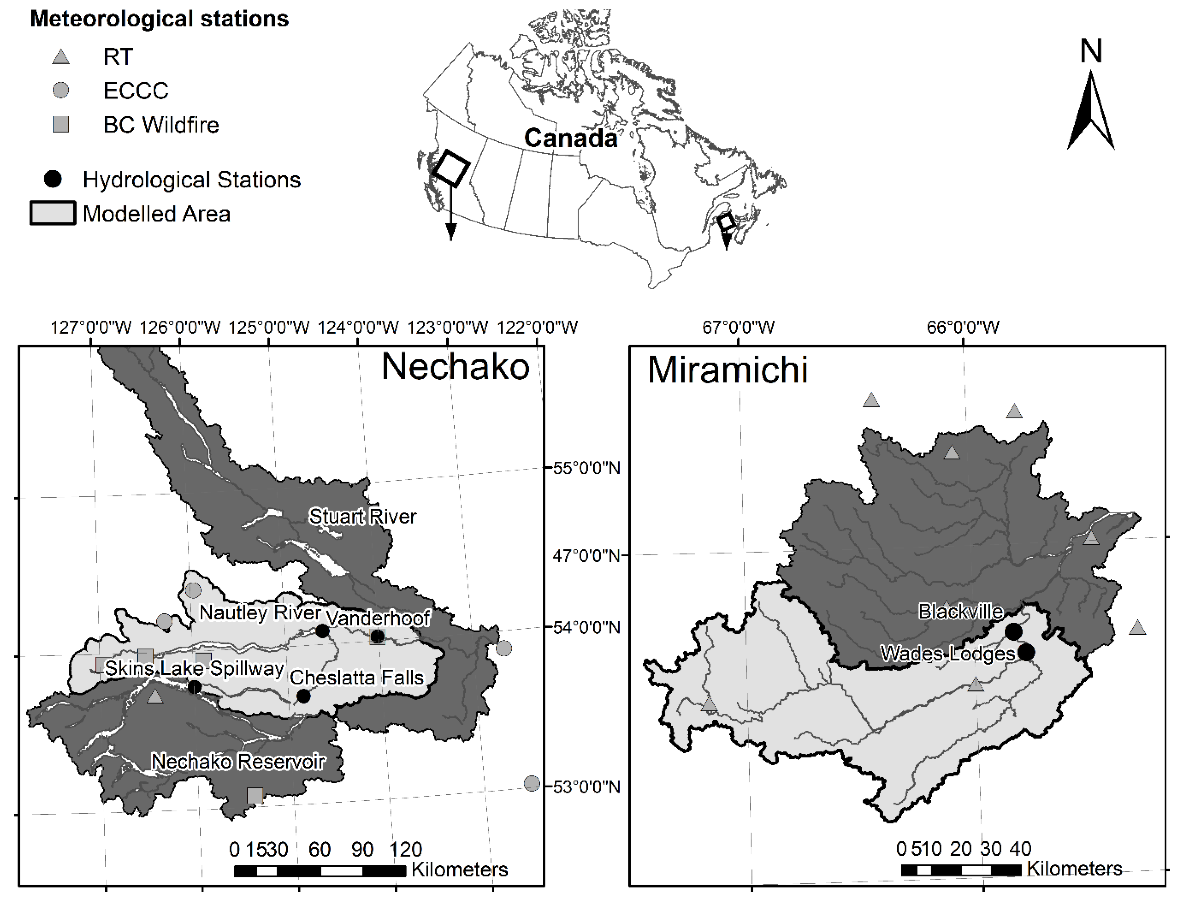
The CEQUEAU model described above was implemented on the Nechako watershed (125°59’ W and 53°46’ N) in the province of British Columbia, Canada and on the Southwest Miramichi River (65°82’ W and 46°74’ N) in the province of New Brunswick, Canada (Figure 2).
2.5.1. Nechako
The Nechako River flows from the Skins Lake Spillway eastward for about 245 km before it reaches its junction with the Stuart River. It begins its course in the coastal range, and then it drains the Nechako Plateau and flows into the Fraser River at Prince George, British Columbia. The elevation of the watershed ranges from 630 m to 1810 m. The watershed covers about 47,000 km2. The Stuart and Nautley Rivers are its major tributaries (Figure 2). A major dam in the Nechako Canyon and nine saddle dams were built in the early 1950s to create the Nechako reservoir, which is about 181 kilometers long [42]. The Skins Lake spillway (Figure 2) typically discharges between 170 and 283 m3/s from 11 July to 20 August and between 14.2 and 49 m3/s throughout the rest of the year.
An average total annual precipitation of 417 mm was monitored at the Ootsa Lake meteorological station between 1981 and 2010, 37% of which fell as snow. The average air temperature is 3.2 °C with an average maximum of 19.8 °C occurring in August and an average minimum of −11.8 °C in January.
A protocol called the Summer Temperature Management Program (STMP) was implemented in the Nechako River to monitor water temperature downstream from the dam and to ensure that water temperature remains below 20 °C at a control section near the city of Finmoore (i.e., upstream of the confluence of the Nechako and Stuart Rivers). This protocol is in effect between 20 July and 20 August (Nechako Fisheries Conservation Program (NFCP), 2005). The measure was introduced to benefit sockeye salmon (Oncorhynchus nerka) during its spawning period. During that period, water releases at Skins Lake are increased in order to reach a minimum discharge of 170 m3/s at Cheslatta Falls. Discharge is then maintained between 170 m3/s and 283 m3/s. When the 20 °C threshold is expected to be exceeded, discharge at the Skins Lake Spillway is increased to 453 m3/s. This operation rapidly increases discharge of the Nechako River downstream and limit its warming at its confluence with the Stuart River. The decision to whether of not increase released discharge at the Skins Lake Spillway is based on a water temperature forecast. To assess the capacity of the model to predict the exceedance of the 20 °C threshold, a Brier Score (Equation (14)) was calculated for values of 20 °C identified as critical temperature (TH). A Brier Score for a threshold value of 18 °C was also calculated and labeled as early warning (EW).
The model was set up for the management of summer water releases at the Skins Lake Spillway. Therefore, only the portion of the watershed located between the Skins Lake Spillway and the confluence of the Nechako and Stuart Rivers (Figure 2) was modeled. At its upstream boundary, the model was fed with the discharge released at the Skins Lake Spillway. Water temperature was also necessary at the model upstream boundary. Data were available for 2013 and 2014 but modeling was required to provide input reservoir temperatures for previous years (2009–2012). An autoregressive model with exogenous variables (ARX) that uses air temperature residuals as predictors [43] was calibrated using data from moored thermographs. The calibrated model was subsequently used to generate water temperature at the surface of the reservoir. Model performances are presented in the results section.
The travel time between the Spillway and the site that is subject to the thermal constrain is estimated to be 5 days [44]. Discharge and water temperature at the outlet of the Nautley River were kept constant for all forecasting horizons (hz1 to hz5) in forecasting mode. The last observation of both discharge and water temperature recorded at the Nautley station (Figure 2) were thus fed to the model. This was done in order to replicate the actual forecasting framework used for operations.
2.5.2. Southwest Miramichi
The Southwest Miramichi flows in the main stem of Miramichi River before it empties in the Atlantic Oceans. It occupies about 60% (7800 km2) of the total drainage area (13,000 km2) of the Miramichi watershed. The elevation of the watershed ranges from sea level to 640 m. Measurement sites are located at Blackville (discharge) and Wades Lodges (water temperature) which drains about 5600 km2. The two measurement sites are separated by 10 km of river. Mean discharge at the Blackville hydrological station (Figure 2) is 120 m3/s with peaks reaching more than 2000 m3/s and low flows around 20 m3/s. Its hydraulic regime is considered as naturel by the Water Survey of Canada (http://wateroffice.ec.gc.ca). It receives an average total precipitation of 1175 mm (Doaktown – Environment and Climate Change Canada) of which 25% falls as snow.
Water temperatures in the Miramichi system are known to exceed the optimal range of 16–20 °C for Atlantic salmon (Salmo salar) [45]. Between 1997 and 2016, mean daily summer water temperature recorded in the Southwest Miramichi was 19.33 °C with a maximum of 25.87 °C (9 July, 2010) and a minimum of 11.36 °C (21 September 2014). Thresholds of 20 °C for minimum daily water temperature and 23 °C for maximum daily water temperature were identified for management strategies in the system [46]. Brier Scores were therefore calculated for thresholds values of 20 °C (early warning) and 23 °C (critical temperature).
Since the Miramichi is unregulated, no input discharge or water temperatures had to be provided to the model as a boundary condition. The period between 15 June and 5 July 2011 on the Miramichi were removed from the analysis because the radiation forecasts were not available. For ease of reading, the Southwest Miramichi will be referred to as the Miramichi.
2.5.3. Meteorological and Hydrological Data
On the Nechako, meteorological data used to adjust the hydrological model parameters (pTot, tMin and tMax) were provided by British Columbia Wildfire (BC Wildfire) management branch, Environment and Climate Change Canada (ECCC) and Rio Tinto (RT), an aluminum producer who manages the watershed for hydropower production (Figure 2). BC Wildfire data were preferred over most of the data from RT’s meteorological stations because of their better representation of the meteorological conditions on the watershed. Cloud cover (CC) was retrieved from ECCC stations Bella Coola, Quesnel, Prince George and Terrace. Net solar radiation (Rs), relative humidity (RH) and wind speed (U) were extracted from the NASA Prediction of Worldwide Energy Resource (POWER) on a grid with 1° horizontal resolution.
A string of 13 temperature loggers (Onset HOBO Pendant temperature loggers; ±0.53 °C accuracy) placed at a 0.91 m (3 feet) vertical distance from each other was attached to a buoy, located at about 150 m upstream of the Skins Lake Spillway from May to October 2013 and 2014 and for July to October during the summer of 2015. These data confirmed that the water column was well mixed during the period of the year where the STMP applies. Data from the first two sensors from the surface were used to calibrate the ARX surface water temperature model in the reservoir, which is subsequently used as the upstream thermal boundary condition. Water temperature time series for Vanderhoof (station #08JC001) and Cheslatta Falls (station #08JA017) were provided by the Water Survey of Canada. On the Nechako River, the calibration dataset for the model includes time series from 2002 to 2006 while the validation period includes years 2007 to 2010. The forecasting period is 2009–2014.
On the Miramichi, pTot, tMin and tMax were provided by Environment and Climate Change Canada (ECCC), and net solar radiation, relative humidity and wind speed were also extracted from the POWER database. CC was derived from the proportion of extra-terrestrial solar radiation reaching the earth surface. All of the aforementioned data were downscaled to the grid used by CEQUEAU using a three nearest neighbors method.
Discharge data at Blackville (station #01BO001) were retrieved from the Water Survey of Canada database. Water temperature data from Department of Fisheries and Oceans Canada at the Wades Lodges station (46.6716 N and 65.7738 W) retrieved from the rivTemp database (http://rivtemp.ca) were used. Gaps in the data were filled using corrected data from Millerton station (46.8779 N and 65.6639 W). The calibration dataset for the model spanned from 2000 to 2005 and the validation dataset spanned from 2006 to 2010. The forecasting period was also 2009–2014 on the Miramichi watershed. These periods were limited by the availability of the water temperature time series and the availability of the observed meteorological inputs.
On both watersheds, RH and mean daily air temperature (Ta; °C) were used to estimate air vapor pressure (ea; kPa) with [47] formula as given by Equations (15) and (16).
The ensemble meteorological forecasts were extracted in grib2 format through The Observing System Research and Predictability Experiment (THORPEX) Interactive Grand Global Ensemble (TIGGE) portal. They include variables that are typically used for the purpose of hydrological forecasting, namely, total precipitation, and minimum and maximum air temperature. In this study the net solar radiation, dew point temperature, wind speed, and cloud cover are also required. These additional variables are used by the thermal model that follows the hydrological model in the modeling/forecasting cascade. Forecasts for the relative humidity are not available on the TIGGE portal. Therefore, the dew point (Td; °C) was used to estimate air vapor pressure (ea; kPa) using Equation (15) with Td replacing Ta. The two orthogonal vectors for wind speed, 10u (east–west axis) and 10v (north–south axis), were transformed in a single wind component.
Forecasts emitted by the Canadian Meteorological Center (CMC) were preferred, as they are the most susceptible of being used operationally in Canada. However, CMC’s net solar radiation forecasts are not available on the TIGGE portal. Consequently, net solar radiation forecasts from the European Centre for Medium Range Weather Forecasts (ECMWF) were used. Forecasts for all other variables are from the CMC. The Canadian ensemble forecasts are composed of 20 members (K = 20) generated from different initial conditions of the atmosphere, physical parameters and perturbed observations [48]. ECMWF forecasts are composed of 50 members also generated from different initial conditions and model’s physics perturbations. In order to use the ECMWF and CMC forecasts in the same forecasting framework, only 20 members out of the 50 emitted by the ECMWF were retained for each forecast (hz1 to hz5). At each time step, a sub-sample of 20 members was drawn randomly and kept for the five forecasting horizons. Another random sub-sample was then drawn for the subsequent time step. All forecasts were extracted at a 0.6° horizontal resolution and downscaled on the CEQUEAU grid using a bilinear interpolation. A CEQUEAU grid resolution of 5 km was used for Nechako watershed and 12 km for the Miramichi watershed. The difference between the grid resolutions is due to the use of pre-existing structures. Previous work by Dugdale et al. [49] showed minor differences in model performance between grids resolutions of 2.5 km and 20 km.
A MCRPS (Equation (12)) was calculated between observations at the meteorological stations and the corresponding grid cell of the meteorological forecasts for tMin, tMax, pTot and Rs. Note that MCRPS for Rs was only calculated for 2014 (25 July to 20 August) on the Nechako watershed. With regards to the remaining Rs forecast and the other input variables (CC, U and ea), MCRPS was calculated by comparing data interpolated on the CEQUEAU grid including data extracted from the POWER database with the forecasts interpolated on the same grid. This was done in order to assess the quality of ensemble meteorological forecasts used as inputs for the hydrological and thermal models. A particular attention was paid to solar radiation because of its importance in the estimation of the surface thermal budget of a river.
3. Results
3.1. Model Calibration and Evaluation
Hydrological and water temperature model calibration performance metrics are summarized in Table 1. Both model show satisfactory performances, with relatively low RMSE values for simulated water temperatures during the critical summer period. The parameters of the thermal model were optimized to best reproduce water temperature at Vanderhoof (Nechako) and Wades Lodges (Miramichi) during the summer period (15 June to 15 September). This was successfully achieved, with a RMSE under 1.6 °C during both calibration and validation periods Table 1). The ARX model (temperature of the water release; see Section 2.5.1.) yielded a RMSE of 1.18 °C and 1.28 °C in calibration and validation, respectively.
3.2. Meteorological Forecasts Evaluation
The MCRPS calculated for the meteorological forecasts are summarized in Table 2. Total precipitation showed relatively low MCRPS for all lead times on both watersheds, ranging between 0.7 mm (hz1—Nechako) to 3.0 mm (hz5—Miramichi). With regards to air temperature, a higher MCRPS was found for tMin (1.97–3.80 °C) compared to tMax (1.35–1.81 °C). Between 25 July and 20 August, MCRPS for Rs ranges between 2.5 MJ/m2 (hz1) and 3.1 MJ/m2 (hz5) at Skins Lake on the Nechako watershed. In relative terms, it represents 13% and 21% of the observed values, respectively. Troccoli and Morcrette [50] calculated relative MAE’s between 18% and 45% for direct solar radiation forecasted by the ECMWF’s Global Atmospheric Model in Australia. These values are of the same order of magnitude than those obtained in the present study.
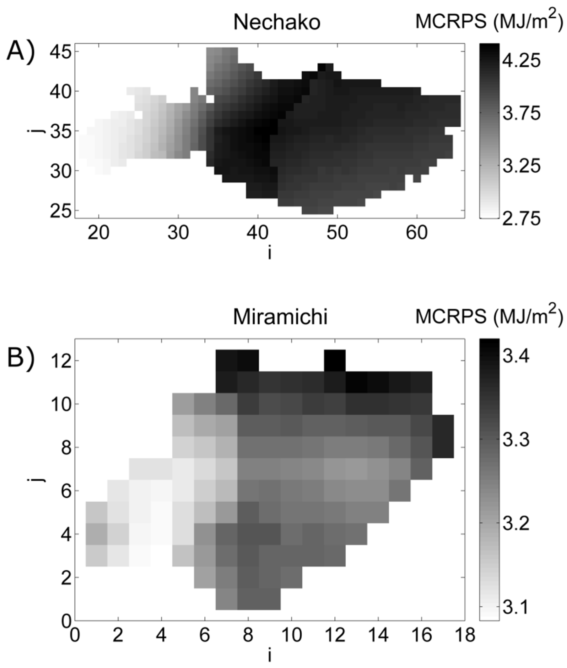
Figure 3 shows MCRPSs calculated between the forecasted radiation interpolated (hz5) on the CEQUEAU grid and the corresponding observations interpolated on the same grid. For ease of reading, only radiation is presented because of its major importance for thermal modeling. Figure 3A highlights an east–west gradient of the adequacy between the grid of observed and forecasted solar radiation on the Nechako watershed. Lower MCRPS values were found in the western section of the watershed while higher values were observed in the middle section before it diminishes again towards the eastern part. In the eastern section, where sits the main stem of the Nechako, MCRPSs remained fairly high with values above 3 MJ/m2. Although not shown here, such an east–west gradient was observed for all forecasted variables.
On the Miramichi watershed, the MCRPS values are slightly higher in the northeastern part of the watershed but no clear spatial pattern was observed with respect to the accuracy of the solar radiation forecast (Figure 3B) or other forecasted meteorological variables. As observed for the Nechako watershed, the MCRPS for solar radiation is quite high across the watershed and remained above 3 MJ/m2.
On the Nechako watershed, the total precipitation showed large relative bias (>100%). In absolute terms, this bias remained fairly low (<2 mm) while the same metrics were much lower on the Miramichi watershed with relative biases under 25% (<1 mm). With regards to air temperature, both tMax and tMin had a relative bias under 20% on both watersheds, which translates into a larger bias for tMax in absolute terms (>3 °C) compared to tMin (<1 °C). On the Nechako watershed, maximum air temperature was strongly biased in the upper part the watershed while bias diminishes towards its eastern border. Air temperature is used in the estimation of longwave radiation (Equation (4)), convection (Equation (7)) and evaporation (Equation (8)). Cloud Cover (CC) on the Nechako watershed showed a positive bias of 32% which was higher in the eastern part of the watershed than in the western part. On the Miramichi maximum biases of 20% were calculated and were constant across the watershed. Forecasted ea had a maximum relative bias of 30% on the Nechako watershed while it reached 12% on the Miramichi. The highest bias values were found in the lower eastern part of the Nechako watershed and were spatially constant on the Miramichi. CC and ea are both used in the calculation of sky emissivity (Equation (4)), involved in the estimation of energy fluxes associated with longwave radiation (Equation (5)). Wind speed, which is used along with air temperature in the calculation of convective heat fluxes (Equation (7)), was biased by 35% (2.5 km/h) on average with a stronger bias in the upper part of the Nechako watershed. On the Miramichi watershed, biases were constant around 15% (1.2 km/h). Solar radiation, used directly as heat input in thermal modeling, was positively biased by 17% (3.14 MJ/m2) on the Nechako watershed and negatively biased by 6% (−1.07 MJ/m2) on the Miramichi watershed.
3.3. Hydrological and Thermal Forecasts Evaluation
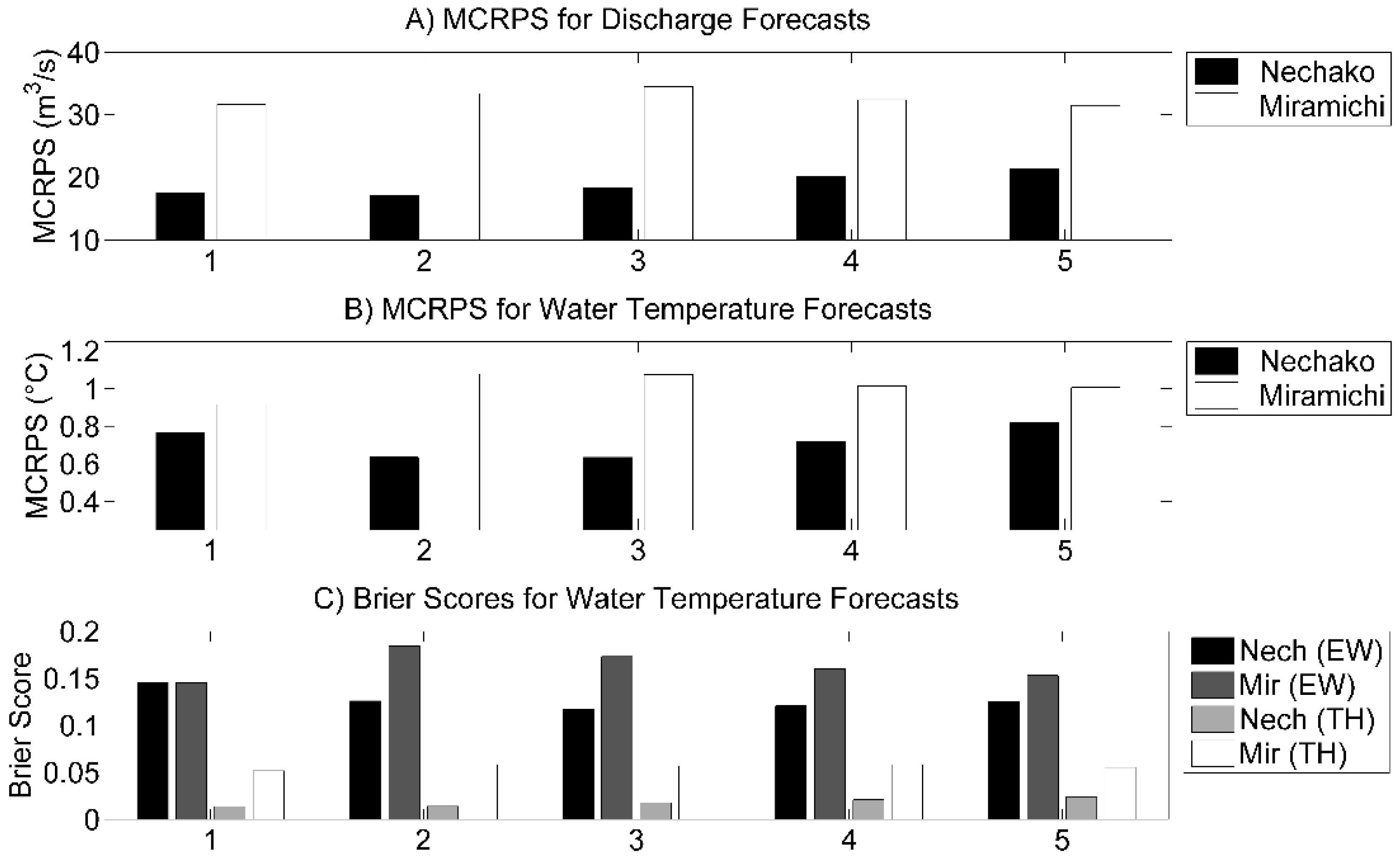
The first step of the forecasting cascade is the hydrological forecast. Since discharge was imposed at the Skins Lake Spillway and at the outlet of the Nautley River in forecasting mode, very low uncertainty (<1 m3/s) was induced to the hydrological forecast by the ensemble precipitation forecast on the Nechako watershed (Figure 4). Therefore, MCRPSs calculated from resulting discharge ensembles (Figure 5A), which range from 17.1 m3/s (hz1) to 21.4 m3/s (hz5) are very similar to MAE calculated from simulations using observed meteorological inputs (17.7 m3/s). On the Miramichi, MCRPSs ranging between 31.7 m3/s (hz1) and 34.4 m3/s (hz3; Figure 5B) were in the same order of magnitude than the MAE calculated on for simulated discharge (34.9 m3/s).
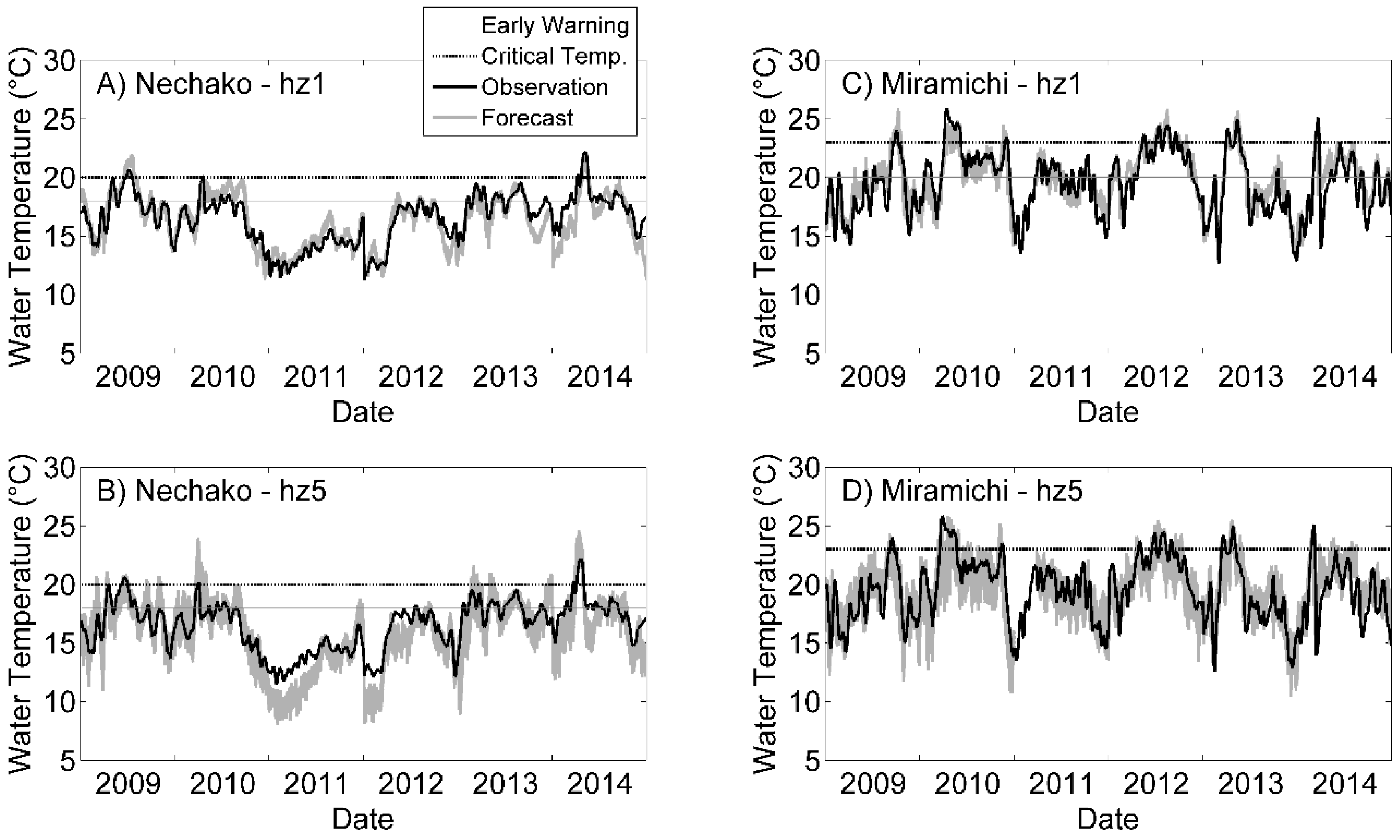
Figure 6 presents the ensemble water temperature forecasts produced on both watershed for one-day-ahead and five-day-ahead lead times. One-day-ahead forecast showed good performances on both rivers with a MCRPS somewhat higher on the Miramichi (0.92 °C) than on the Nechako (0.77 °C) but both under 1 °C (Figure 5B). The spread of the ensemble was also larger on the Miramichi (0.92 °C) than on the Nechako (0.73 °C). On the Nechako, the MCRPS increased with lead time to reach 0.82 °C on hz5. On the Miramichi, MCRPS reaches 1.08 °C on hz2 and decreases to 1.00 °C on hz5. Figure 6B shows that some five-day lead time forecasts are strongly biased at the beginning of 2011 and 2012 on the Nechako.
In terms of threshold exceedance predictions indicated by the BS, similar values for the early warning were obtained for both rivers with BS = 0.15 for hz1 (Nechako and Miramichi) and respectively 0.13 and 0.15 for the Nechako and the Miramichi at hz5 (Figure 5C). When the BS is calculated for higher temperature thresholds (critical temperature), both rivers performed well with lower scores obtained on the Nechako (BS = 0.01 − 0.02) compared to Miramichi (BS = 0.05 − 0.06). Both thresholds were represented on Figure 6. Over the forecasting period, the early warning temperature was exceeded on 46% of the time on the Miramichi and 24% on the Nechako and the critical temperature was exceeded 10% of the time on the Miramichi and 3% on the Nechako.
3.4. Uncertainty and Reliability of the Forecasts
One of the main objectives of this work is to assess and represent the uncertainty that is propagated to a water temperature forecast by the meteorological inputs. Figure 4 shows that the spread of the discharge ensemble forecast is much larger on the Miramichi than on the Nechako with values between 3.74 m3/s and 125.9 m3/s. Important variability was observed during the forecasting period, especially for longer lead times with a standard deviation of 194 m3/s for hz5 (Figure 4).
Figure 7 shows the spread of the water temperature ensemble forecasts. The central line displays the mean spread of the ensemble for a given lead time and the vertical bars represent one standard deviation of the same spread. We observed a larger ensemble spread on the Miramichi compared to the Nechako for both forecasting horizons. On both rivers, the spread of the ensemble increased with lead time to reach 2.29 °C on the Nechako and 3.14 °C on the Miramichi. However, the spread of the ensemble as well as the variability of the spread increased more rapidly on the Miramichi than on the Nechako (Figure 7). Therefore, more uncertainty was propagated in the Miramichi water temperature forecasting system. These observations are also visible on the time series plot on Figure 4. It should be noted that the water temperature forecasts spread on the Miramichi is exacerbated by the propagation of the uncertainty of the discharge forecast to the water temperature forecast.
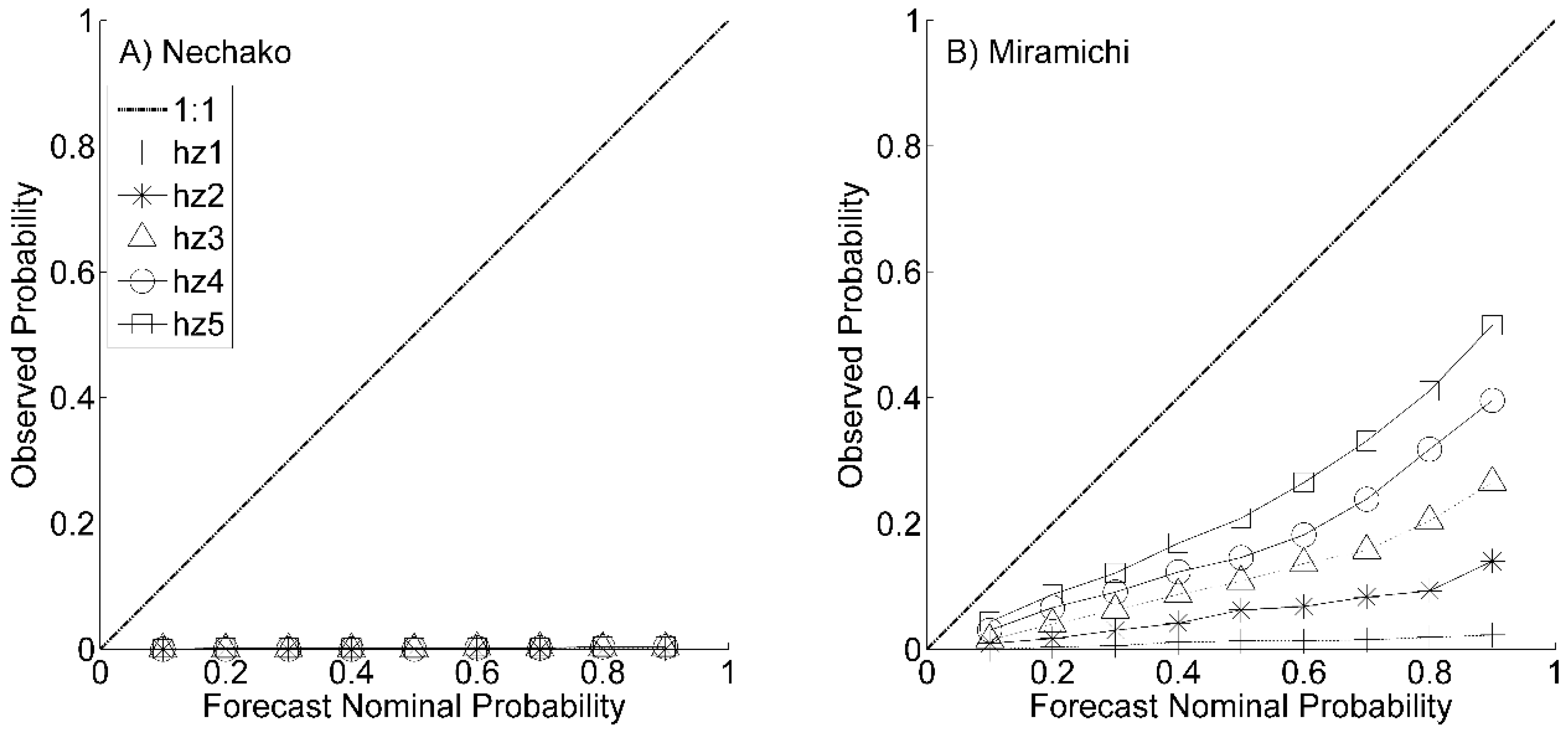
Figure 8 shows the reliability plots of discharge forecasts for all lead times. The reliability plot for the Nechako (Figure 8A) clearly demonstrates the lack of spread of the discharge forecast. For all forecasting horizons, the observed probabilities stay close to zero for all forecast nominal probabilities. This indicates that observed discharge almost never falls into the ensemble and that the forecasting framework does not include enough uncertainty to be reliable. On the Miramichi (Figure 8B), the reliability increases constantly with lead time. Although the reliability of the discharge forecast is better on the Miramichi than it is on the Nechako, the lines being under the bisector indicates an under-dispersion of the ensemble. For a forecasted probability of 0.9, the observed probability goes from 0.02 (hz1) to 0.5 (hz5). Although a clear surge in reliability was visible between the first and the fifth horizon, the observed probability remained lower than the forecasted probability for all levels of confidence.
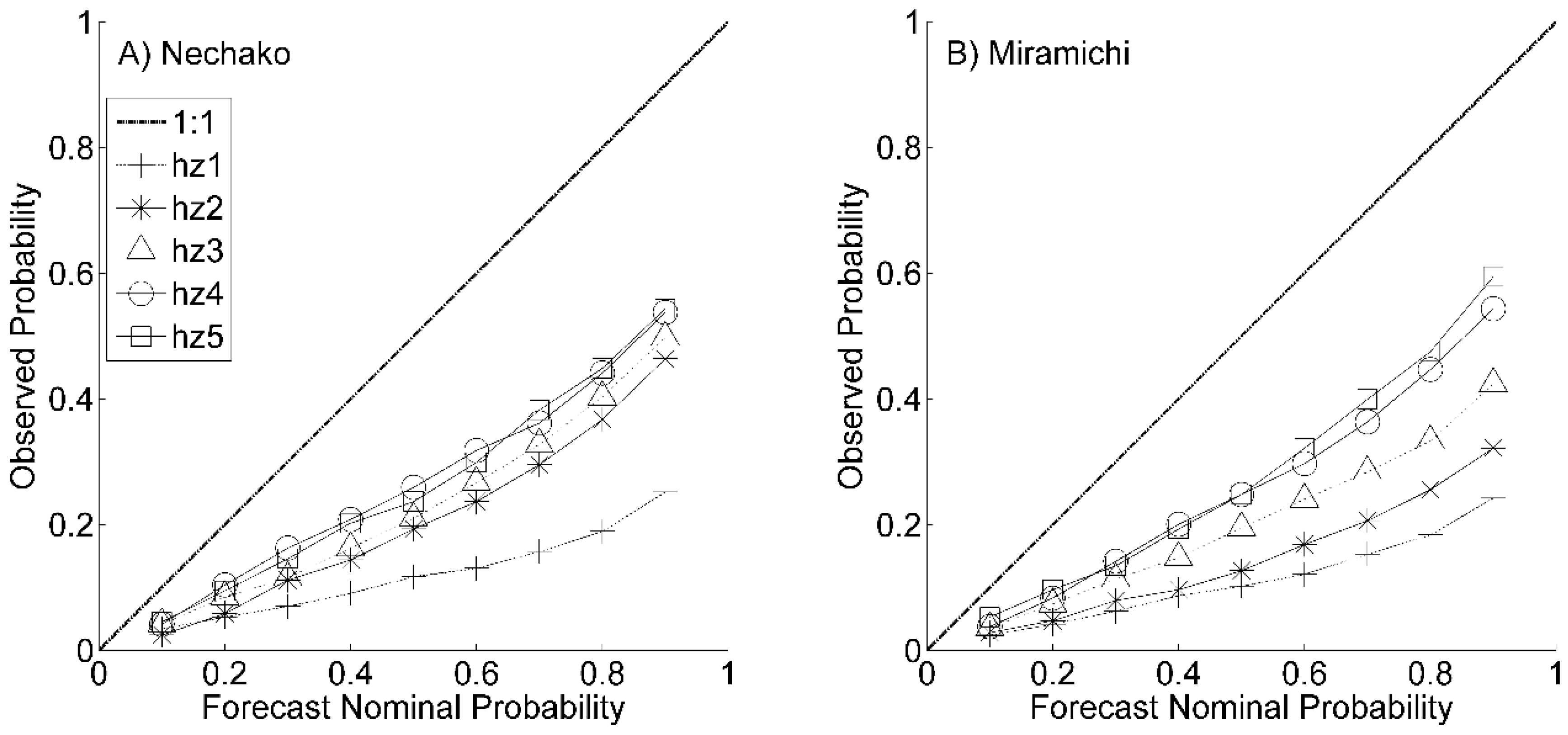
Figure 9 displays the reliability plots for water temperature forecasts for all forecasting horizons. It can be seen that on both rivers reliability increases with lead time. However, more disparity is visible between hz1 and hz5 on the Miramichi. For a nominal probability of 0.9 the observed probability goes from 0.24 to 0.59 while it goes from 0.25 to 0.54 on the Nechako. In both cases, this suggests an over-confidence of the forecasts, meaning that the spread of the ensemble is narrower than it should be in order to convey the total uncertainty related to the forecasting situation. The ensembles of all five lead time forecasts are thus found to be under dispersed.
4. Discussion
In this paper, we produced five-day-ahead forecasts on two Canadian watersheds with special emphasis directed towards uncertainty of meteorological inputs. As expected, the spread of the water temperature ensemble, representative of the meteorological and hydrological uncertainty propagated within the forecast, grows larger with the forecasting horizon. This translated into an improvement in reliability with lead time. This improvement of reliability results from an increase in uncertainty rather than from a better accuracy of the forecast. As demonstrated in Section 3.2, meteorological forecasts for all variables were diagnosed as biased. Obviously, the best way to improve the reliability of forecasts is to correct those biases. However, this operation was left out of the present study for two reasons: first, there is a certain disagreement among the hydrologic ensemble forecasting community as to whether it is better to pre-process meteorological inputs, or post-process the hydrological forecasts to remove bias. For instance, Kang et al. [51] showed that post-processing was much more efficient than pre-processing to improve the quality of their final streamflow forecasts. Verkade et al. [52] found that pre-processing meteorological forecasts to remove bias and correct dispersion resulted in very little gain, if any at all, for the final streamflow forecasts. To the best of our knowledge, a comparative study between pre- and post-processing was never undertaken in the context of water temperature forecasting, since ensemble forecast and quantification of uncertainty is a very new topic to this field. Second, many different pre- and post-processing methods exist, spanning from very simple [53] to more elaborate (e.g., Bayesian Model Averaging [54]). An adequate comparison of methods is outside of the scope of the present study, which is a first attempt at assessing the potential of ensemble forecasts in the context of water temperature. An in-depth comparative study on the merits of various methods for pre- and post-processing to improve the reliability of water temperature forecasts is a potential subsequent research avenue.
On the Nechako watershed, despite the large MCRPS for the ensemble precipitation forecasts (2.8 mm at hz5), the effects of this uncertainty on the forecasted discharge are very small. This is due to the fact that discharge is imposed at the model upstream boundaries, namely the Skins Lake Spillway and the outlet of the Nautley River. The large spread observed in forecasted water temperatures for the unregulated Miramichi, even for the first forecasting horizon, suggests an influence of the precipitation uncertainty that propagates into the discharge and ultimately to the water temperature forecasts. This indicates the apparent consequences of the quality of the precipitation forecasts on the subsequent hydrological and thermal forecasting in a natural river. Naturally, the uncertainty propagated within the discharge forecast is transferred to the water temperature forecast. Further analysis would be required to quantify in details this propagation of precipitation uncertainty across the model cascade. Since the volume of water is included in the estimation of water temperature (Equation (1)), the uncertainty of the precipitation, propagated to the discharge, induces uncertainty to the water temperature forecasts. In a regulated system, like the Nechako River, this influence is highly tempered by flow regulation in opposition to a natural system, like the Miramichi River, where surface runoff freely reaches the hydrological network.
Solar radiation (Rs) is known to be the dominant variable of the energy budget in most rivers [7] while being a direct output of atmospheric models. Error in Rs values should therefore be a dominant contribution to the total uncertainty of energy fluxes. However, additional work, including a detailed analysis of each forecasted flux, would be required confirm this hypothesis. Surprisingly, the ensemble forecast’s accuracy (MCRPS) and its capacity to predict a threshold exceedance (BS) remained fairly constant with lead time. Both metrics (CRPS and BS) were expected to increase indicating a lower accuracy and threshold exceedance prediction capacity. This can be explained by the fact that the initial conditions of the watershed at the beginning of the forecast are estimations dependent on the spin up period and are necessarily uncertain themselves. The ensemble forecasts were produced from initial states generated from simulations with observed meteorological conditions as inputs without the assimilation of the observed hydrological and thermal conditions. Therefore, the thermal inertia of the system limits the deviation of the short-term forecasts from the initial conditions. Thiboult et al. [24] showed the important influence of the initial conditions of the watershed on hydrological forecast accuracy and reliability through data assimilation. They also suggested that these initial conditions mostly influence the quality of the forecasts for shorter lead times. In the present study, results indicate that the lower reliability for shorter lead times can be attributable to the absence of data assimilation. This is especially visible for the discharge forecast on the Nechako River where a relatively narrow ensemble spread translates into low reliability forecasts. Although the proposed model shows satisfactory performances in both calibration and validation modes, initial states still carry a modeling error. In this case, the thermal inertia of the system will carry this modeling error through the forecast horizons but will dissipate with lead time. Although the proposed forecasting framework performed well in both a regulated and an unregulated river system, the problem related with initial states uncertainty should also be addressed in future work.
The MAE obtained from archived deterministic operational forecasts using a one-dimensional unsteady state water temperature model on the Nechako (personal communication [55]; Table 3) for a one-day-ahead forecasts was lower (MAE = 0.49 °C) than those obtained in the present study but only spanned from 20 July to 20 August and did not include 2011 and 2012. For the same forecasting period and the same years, the proposed framework yields a MCRPS of 0.85 °C. However, for a five-day-ahead forecast, performance is very similar to the archived, with the archived forecasts having a MAE of 0.68 °C while the proposed framework yielded a MCRPS of 0.69 °C. Forecasts were also produced on a tributary of the Southwest Miramichi, the Little Southwest Miramichi (LSWM), by Caissie et al. [56]. An autoregressive models with air temperature as an exogenous variables (ARX) was used for 1–3-day lead times from 1992 to 2011 during the summer (June–September). Results shows RMSE of 0.87 °C for one-day-ahead forecast and 1.48 °C for a three-day-ahead forecast (Table 3). For the same lead times, the proposed method returned MCRPS of respectively 0.92 °C and 1.07 °C. Although both metrics cannot be directly compared, these results suggest a slightly better performance of the ARX model for a one-day-ahead forecast but a better performance of our proposed method for a three-day-ahead forecast. Although the main objective of this paper is to highlight the uncertainty associated with meteorological inputs in a hydrological and thermal forecast, these comparisons suggest a good potential of CEQUEAU to produce five-day lead time forecasts with reasonable accuracy. A thorough model comparison would be of interest for future work.
All forecasts carry uncertainty from various sources. In the absence of knowledge on this uncertainty, the level of confidence into a forecast can hardly be estimated. One of the aims of this study was to provide information on the uncertainty from eight input variables from an atmospheric model that propagates to water temperature forecast in both a regulated and a natural river. We showed the satisfactory accuracy of the ensemble forecast and its capacity to accurately predict threshold exceedance for management purpose for a one to five-day lead time. From a management point of view, these good performances on longer lead times are valuable, given the fact that decisions and management strategies can be better adapted with longer lead time. Knowledge of the uncertainty associated with a water temperature forecast is also valuable and should be integrated in decision making processes. This can be done by basing decisions (at least in part) on probabilistic forecasts like those proposed in the present study. Such framework helps to explicitly communicate the risk associated with a decision. In this case, the probability of exceedance of the water temperature threshold can be calculated from the ensembles. For instance, when five out of 20 members predict the exceedance of 20 °C water temperature for a given water release, then the risk of having a threshold exceedance is 25%. A decision therefore can be made based on knowledge of the risk associated with this decision. In fact, it was recently shown that the level of risk aversion of a decision-maker is a key factor in assessing the comparative benefits of forecasting systems for decision-making [57]. In the case of a fully deterministic forecast, that notion of risk is much more difficult to assess and to communicate to the decision-makers, although they are usually aware of its existence [58]. From this point of view, ensemble forecasts are clearly advantageous over deterministic forecasts and can even be seen as more “complete”.
While understanding of the uncertainty associated with meteorological inputs was improved with this study, further work is required to fully and accurately capture the uncertainty in water temperature ensemble forecasts, especially for short lead times (1–3 days). The lack of reliability associated with these forecasts also suggests that uncertainty sources that dominate for short lead times have yet to be fully understood and incorporated in the forecasting framework. Among other sources, the choice of particular hydrological and thermal models, initial conditions, and the level of model parameterization are known to induce uncertainty to the hydrological modeling/forecasting [59]. The combination of ensemble forecasting approaches (data assimilation, multi-model and ensemble meteorological forecasts) was shown to be effective to properly represent uncertainty over short- (one day) to long-term (10 days) hydrological forecasts [24]. River temperature forecasting would likely benefit from a similar, more complete approach.
5. Conclusions
The study presented in this paper proposes a modeling framework used to produce ensemble water temperature forecasts in a regulated and a natural river system. Uncertainty associated with meteorological forecast inputs was quantified throughout the forecasting process. The resulting water temperature forecasts showed good performances on both watersheds for a five-day lead time with a better accuracy on the regulated river system (Nechako) and a better reliability on the natural river system (Miramichi). The present study improved our knowledge of the risk associated with water temperature forecast. As far as the authors know, this paper represents the first published attempt to produce ensemble water temperature forecasts by feeding ensemble meteorological forecasts to a hydrological and thermal model cascade. Further work is required to address accuracy and reliability of short-term ensemble forecasts (1–3 days). Structural uncertainty and initial state error should thus be investigated in combination with ensemble meteorological forecasts in future work in water temperature forecasting.
Acknowledgments
This work was funded in part by NSERC and Rio Tinto. The authors wish to thank J. Benckhuysen B. Larouche and M. Latraverse for their assistance in the realization of this project. They also wish to thank the ECMWF for maintaining the TIGGE portal that provides free access to ensemble meteorological forecasts for research purposes. Water temperature data from the Southwest Miramichi were obtained from D. Caissie (Fisheries and Oceans Canada), who is to be thanked for his assistance.
Author Contributions
All authors participated equally in the elaboration of the experiment. Sébastien Ouellet-Proulx performed the data analysis and prepared the manuscript. André St-Hilaire and Marie-Amélie Boucher reviewed the manuscript throughout the writing process.
Conflicts of Interest
The authors declare no conflict of interest. The founding sponsors had no role in the design of the study; in the collection, analyses, or interpretation of data; in the writing of the manuscript, and in the decision to publish the results.
References
- Fry, F.E.J. The effect of environmental factors on the physiology of fish. Fish Physiol. 1971, 6, 1–98. [Google Scholar]
- Ward, J.V.; Stanford, J.A. Thermal responses in the evolutionary ecology of aquatic insects. Annu. Rev. Entomol. 1982, 27, 97–117. [Google Scholar] [CrossRef]
- McCullough, D.A. Are coldwater fish populations of the United States actually being protected by temperature standards? Freshw. Rev. 2010, 3, 147–199. [Google Scholar] [CrossRef]
- McCullough, D.A.; Spalding, S.; Sturdevant, D.; Hicks, M. Summary of Technical Literature Examining the Physiological Effects of Temperature on Salmonids; US Environmental Protection Agency: Washington, DC, USA, 2001; 119p, ISBN EPA-910-D-01-005.
- Ouellet, V.; Pierron, F.; Mingelbier, M.; Fournier, M.; Marlène, F.; Couture, P. Thermal Stress Effects on Gene Expression and Phagocytosis in the Common Carp (Cyprinus Carpio): A Better Understanding of the Summer 2001 St. Lawrence River Fish Kill. Open Fish Sci. J. 2013, 6, 99–106. [Google Scholar] [CrossRef]
- Sullivan, K.; Martin, D.J.; Cardwell, R.D.; Toll, J.E.; Steven, D. An analysis of the effects of temperature on salmonids of the Pacific Northwest with implications for selecting temperature criteria. Histochemistry 2000, 90, 85–97. [Google Scholar]
- Caissie, D. The thermal regime of rivers: A review. Freshw. Biol. 2006, 51, 1389–1406. [Google Scholar] [CrossRef]
- Maheu, A.; Poff, N.L.; St-Hilaire, A. A Classification of Stream Water Temperature Regimes in the Conterminous USA. River Res. Appl. 2016, 32, 896–906. [Google Scholar] [CrossRef]
- Ward, J.V.; Stanford, J.A. Ecological factors controlling streams zoobenthos with emphasis on thermal modification of regulated streams. In The Ecology of Regulated Streams; Ward, J.V., Stanford, J.A., Eds.; Plenum Press: New York, NY, USA, 1979; pp. 35–56. [Google Scholar]
- Crisp, D.T. Thermal “resetting” of streams by reservoir releases with special reference to effects on salmonid fishes. In Regulated Streams: Advances in Ecology; Craig, J.F., Kemper, J.B., Eds.; Plenum Press: New York, NY, USA, 1987; pp. 163–182. [Google Scholar]
- Poff, N.L.; Hart, D.D. How Dams Vary and Why It Matters for the Emerging Science of Dam Removal. Bioscience 2002, 52, 659–668. [Google Scholar] [CrossRef]
- Gu, R.; Montgomery, S.; Austin, T. Al Quantifying the effects of stream discharge on summer river temperature. Hydrol. Sci. 1998, 43, 885–904. [Google Scholar] [CrossRef]
- Cole, J.C.; Maloney, K.O.; Schmid, M.; McKenna, J.E. Developing and testing temperature models for regulated systems: A case study on the Upper Delaware River. J. Hydrol. 2014, 519, 588–598. [Google Scholar] [CrossRef]
- Benyahya, L.; Caissie, D.; St-Hilaire, A.; Ouarda, T.B.M.; Bobée, B. A Review of Statistical Water Temperature Models. Can. Water Resour. J. 2007, 32, 179–192. [Google Scholar] [CrossRef]
- Pike, A.; Danner, E.; Boughton, D.; Melton, F.; Nemani, R.; Rajagopalan, B.; Lindley, S. Forecasting river temperatures in real time using a stochastic dynamics approach. Water Resour. Res. 2013, 49, 5168–5182. [Google Scholar] [CrossRef]
- Olden, J.D.; Naiman, R.J. Incorporating thermal regimes into environmental flows assessments: Modifying dam operations to restore freshwater ecosystem integrity. Freshw. Biol. 2010, 55, 86–107. [Google Scholar] [CrossRef]
- Breau, C. Knowledge of Fish Physiology Used to Set Water Temperature Thresholds for In-Season Closures of Atlantic Salmon (Salmo salar) Recreational Fisheries; Research Document 2012/163; Fisheries and Oceans Canada: Moncton, NB, Canada, 2012.
- Webb, B.W.; Hannah, D.M.; Moore, R.D.; Brown, L.E.; Nobilis, F. Recent advances in stream and river temperature research. Hydrol. Process. 2008, 22, 902–918. [Google Scholar] [CrossRef]
- Huang, B.; Langpap, C.; Adams, R.M. Using instream water temperature forecasts for fisheries management: An application in the Pacific Northwest. J. Am. Water Resour. Assoc. 2011, 47, 861–876. [Google Scholar] [CrossRef]
- Danner, E.M.; Melton, F.S.; Pike, A.; Hashimoto, H.; Michaelis, A.; Rajagopalan, B.; Caldwell, J.; Dewitt, L.; Lindley, S.; Nemani, R.R. River temperature forecasting: A coupled-modeling framework for management of river habitat. IEEE J. Sel. Top. Appl. Earth Obs. Remote Sens. 2012, 5, 1752–1760. [Google Scholar] [CrossRef]
- Huang, B.; Langpap, C.; Adams, R.M. The value of in-stream water temperature forecasts for fisheries management. Contemp. Econ. Policy 2012, 30, 247–261. [Google Scholar] [CrossRef]
- Casati, B.; Wilson, L.J.; Stephenson, D.B.; Nurmi, P.; Ghelli, A.; Pocernich, M.; Damrath, U.; Ebert, E.E.; Brown, B.G.; Mason, S.; et al. Forecast verification: Current status and future directions. Meteorol. Appl. 2008, 15, 3–18. [Google Scholar] [CrossRef]
- Boucher, M.A.; Anctil, F.; Perreault, L.; Tremblay, D. A comparison between ensemble and deterministic hydrological forecasts in an operational context. Adv. Geosci. 2011, 29, 85–94. [Google Scholar] [CrossRef]
- Thiboult, A.; Anctil, F.; Boucher, M.A. Accounting for three sources of uncertainty in ensemble hydrological forecasting. Hydrol. Earth Syst. Sci. 2016, 20, 1809–1825. [Google Scholar] [CrossRef]
- Cloke, H.L.; Pappenberger, F. Ensemble flood forecasting: A review. J. Hydrol. 2009, 375, 613–626. [Google Scholar] [CrossRef]
- Bartholow, J. Modeling uncertainty: Quicksand for water temperature modeling. Hydrol. Sci. Technol. 2003, 19, 221–232. [Google Scholar]
- Yearsley, J.R. A semi-Lagrangian water temperature model for advection-dominated river systems. Water Resour. Res. 2009, 45, 1–19. [Google Scholar] [CrossRef]
- Hague, M.J.; Patterson, D.A. Evaluation of Statistical River Temperature Forecast Models for Fisheries Management. North Am. J. Fish. Manag. 2014, 34, 132–146. [Google Scholar] [CrossRef]
- Bal, G.; Rivot, E.; Baglinière, J.-L.; White, J.; Prévost, E. A Hierarchical Bayesian Model to Quantify Uncertainty of Stream Water Temperature Forecasts. PLoS ONE 2014, 9, e115659. [Google Scholar] [CrossRef] [PubMed]
- Morin, G.; Couillard, D. Predicting river temperatures with a hydrological model. In Encyclopedia of Fluid Mechanics; Gulf Publishing Compagny: Hudson, TX, USA, 1990; pp. 171–209. [Google Scholar]
- St-Hilaire, A.; Morin, G.; El-Jabi, N.; Caissie, D. Water temperature modelling in a small forested stream: Implication of forest canopy and soil temperature. Can. J. Civ. Eng. 2000, 27, 1095–1108. [Google Scholar] [CrossRef]
- St-Hilaire, A.; Boucher, M.-A.; Chebana, F.; Ouellet-Proulx, S.; Zhou, Q.-X.; Larabi, S.; Dugdale, S. Breathing a new life to an older model: The CEQUEAU tool for flow and water temperature simulations and forecasting. In Proceedings of the 22nd Canadian Hydrotechnical Conference, Montreal, QC, Canada, 29 April–2 May 2015. [Google Scholar]
- Hansen, N.; Ostermeier, A. Adapting Arbitrary Normal Mutation Distributions in Evolution Strategies: The Covariance Matrix Adaptation. In Proceedings of the 1996 IEEE International Conference on Evolutionary Computation, Nagoya, Japan, 20–22 May 1996; pp. 312–317. [Google Scholar]
- Hamill, T.M.; Colucci, S.J. Verification of Eta–RSM Short-Range Ensemble Forecasts. Mon. Weather Rev. 1997, 125, 1312–1327. [Google Scholar] [CrossRef]
- Hersbach, H. Decomposition of the Continuous Ranked Probability Score for Ensemble Prediction Systems. Weather Forecast. 2000, 15, 559–570. [Google Scholar] [CrossRef]
- Laio, F.; Tamea, S. Verification tools for probabilistic forecasts of continuous hydrological variables. Hydrol. Earth Syst. Sci. Discuss. 2006, 3, 2145–2173. [Google Scholar] [CrossRef]
- Gneiting, T.; Raftery, A.E. Strictly Proper Scoring Rules, Prediction, and Estimation. J. Am. Stat. Assoc. 2007, 102, 359–378. [Google Scholar] [CrossRef]
- Gneiting, T.; Raftery, A.E.; Westveld, A.H.; Goldman, T. Calibrated Probabilistic Forecasting Using Ensemble Model Output Statistics and Minimum CRPS Estimation. Mon. Weather Rev. 2005, 133, 1098–1118. [Google Scholar] [CrossRef]
- Macdonald, J.S.; Morrison, J.; Patterson, D.A. The efficacy of reservoir flow regulation for cooling migration temperature for sockeye salmon in the Nechako River watershed of British Columbia. North Am. J. Fish. Manag. 2012, 32, 415–427. [Google Scholar] [CrossRef]
- Brier, G.W. Verification of forecasts expressed in terms of probability. Mon. Weather Rev. 1950, 78, 1–3. [Google Scholar] [CrossRef]
- Stanski, H.; Wilson, L.; Burrows, W. Survey of Common Verification Methods in Meteorology; World Weather Watch Technology Report 8; World Meteorological Organization: Geneva, Switzerland, 1989. [Google Scholar]
- Boudreau, K. Nechako Watershed Council Report: Assessment of Potential Flow Regimes for the Nechako Watershed; 4Thought Solutions Inc.: Vancouver, BC, Canada, 2005. [Google Scholar]
- Ahmadi-Nedushan, B.; St.-Hilaire, A.; Ouarda, T.B.M.J.; Bilodeau, L.; Robichaud, É.; Thiémonge, N.; Bobée, B. Predicting river water temperatures using stochastic models: Case study of the Moisie River (Québec, Canada). Hydrol. Process. 2007, 21, 21–34. [Google Scholar] [CrossRef]
- Envirocon Ltd. Documentation of the Nechako Unsteady State Water Temperature Model; Envirocon Ltd.: Vancouver, BC, Canada, 1984. [Google Scholar]
- Caissie, D.; Breau, C.; Hayward, J.; Cameron, P. Water Temperature Characteristics within the Miramichi and Restigouche Rivers; Research Document 2012/165; Fisheries and Oceans Canada: Moncton, NB, Canada, 2012.
- Temperature Threshold to Define Management Strategies for Atlantic salmon (Salmo salar) Fisheries under Environmentally Stressful Conditions; Canadian Science Advisory Secretariat Science Advisory Report 2012/019; Fisheries and Oceans Canada: Moncton, NB, Canada, 2012.
- Tetens, O. Uber einige meteorologische. Begr. Zeitschrift fur Geophys. 1930, 6, 297–309. [Google Scholar]
- Gagnon, N.; Beauregard, S.; Muncaster, R.; Abrahamowicz, M.; Lahlou, R.; Lin, H. Improvements to the Global Ensemble Prediction System (GEPS) from Version 3.1.0 to Version 4.0.0; Technical Note; Canadian Meteorological Centre: Dorval, QC, Canada, 2014.
- Dugdale, S.J.; St-Hilaire, A.; Curry, R.A. Automating physiography and flow routing inputs to the CEQUEAU hydrological model: Sensitivity testing on the St. John River Watershed. J. Hydroinform. 2017, 19, 469–492. [Google Scholar] [CrossRef]
- Troccoli, A.; Morcrette, J.J. Skill of direct solar radiation predicted by the ECMWF global atmospheric model over Australia. J. Appl. Meteorol. Climatol. 2014, 53, 2571–2588. [Google Scholar] [CrossRef]
- Kang, T.H.; Kim, Y.O.; Hong, I.P. Comparison of pre- and post-processors for ensemble streamflow prediction. Atmos. Sci. Lett. 2010, 11, 153–159. [Google Scholar] [CrossRef]
- Verkade, J.S.; Brown, J.D.; Reggiani, P.; Weerts, A.H. Post-processing ECMWF precipitation and temperature ensemble reforecasts for operational hydrologic forecasting at various spatial scales. J. Hydrol. 2013, 501, 73–91. [Google Scholar] [CrossRef]
- Gudmundsson, L.; Bremnes, J.B.; Haugen, J.E.; Engen-Skaugen, T. Technical Note: Downscaling RCM precipitation to the station scale using statistical transformations—A comparison of methods. Hydrol. Earth Syst. Sci. 2012, 16, 3383–3390. [Google Scholar] [CrossRef]
- Raftery, A.E.; Gneiting, T.; Balabdaoui, F.; Polakowski, M. Using Bayesian Model Averaging to Calibrate Forecast Ensembles. Mon. Weather Rev. 2005, 133, 1155–1174. [Google Scholar] [CrossRef]
- Triton Environmental Consultants. Personal communication, 1 January 2016.
- Caissie, D.; Thistle, M.E.; Benyahya, L. River temperature forecasting: Case study for Little Southwest Miramichi River (New Brunswick, Canada). Hydrol. Sci. J. 2016, 62, 683–697. [Google Scholar]
- Matte, S.; Boucher, M.-A.; Boucher, V.; Fortier Filion, T.-C. Moving beyond the cost-loss ratio: Economic assessment of streamflow forecasts for a risk-averse decision maker. Hydrol. Earth Syst. Sci. 2017, 21, 2967–2986. [Google Scholar] [CrossRef]
- Weijs, S.V.; Schoups, G.; Van De Giesen, N. Why hydrological predictions should be evaluated using information theory. Hydrol. Earth Syst. Sci. 2010, 14, 2545–2558. [Google Scholar] [CrossRef]
- Beven, K.J. Prophecy, reality and uncertainty in distributed hydrological modelling. Adv. Water Res. 1993, 16, 41–51. [Google Scholar] [CrossRef]
Figure 1.
Forecasting framework of discharge and water temperature.
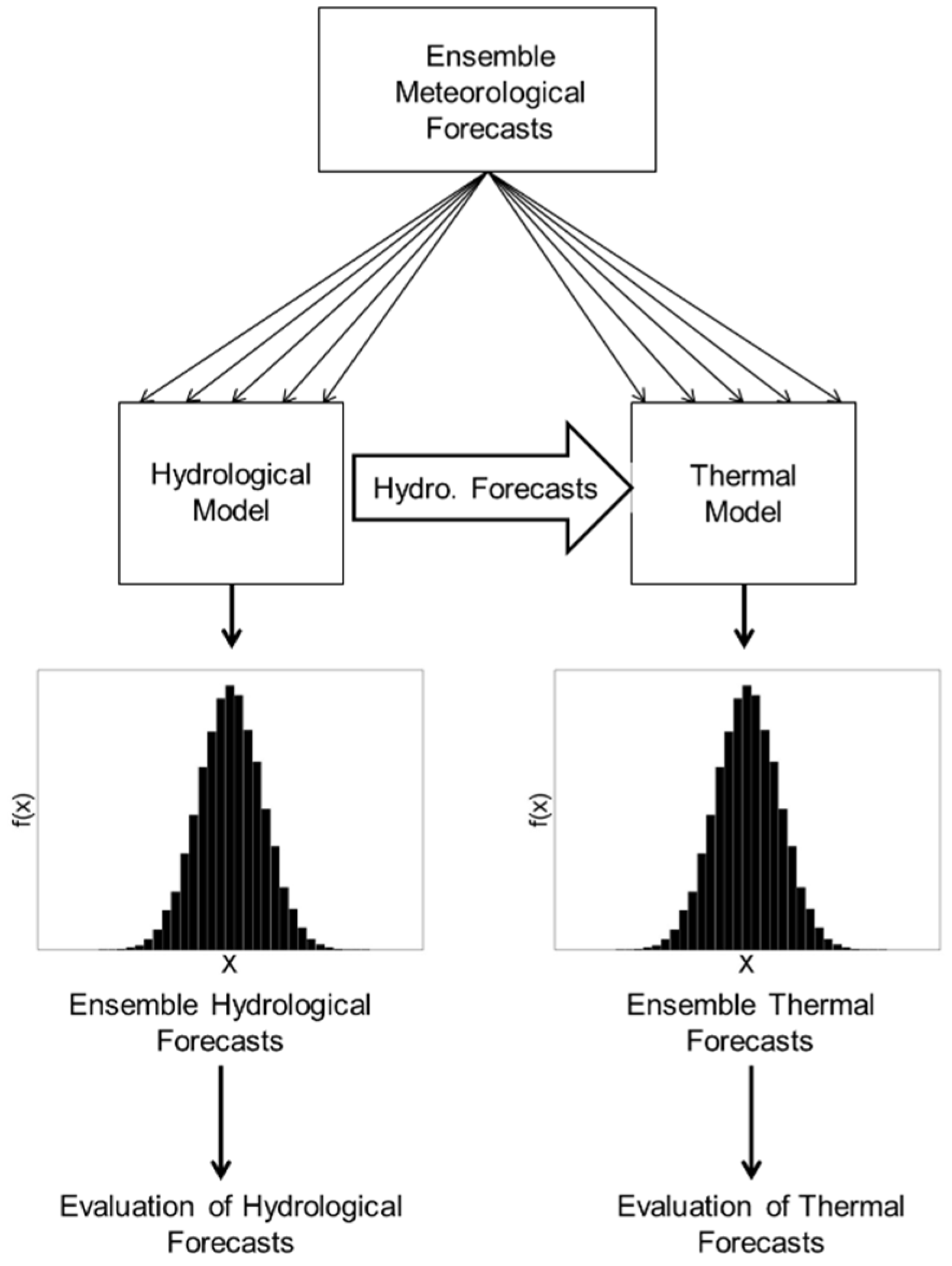
Figure 2.
Maps of the Nechako and the Miramichi watersheds.

Figure 3.
MCRPS of interpolated solar radiation compared to interpolated observations on: (A) the Nechako watershed; and (B) the Miramichi watershed.
Figure 3.
MCRPS of interpolated solar radiation compared to interpolated observations on: (A) the Nechako watershed; and (B) the Miramichi watershed.

Figure 4.
Ensemble discharge forecasts for a: (A) one-day lead time on the Nechako; (B) five-day lead time on the Nechako; (C) one-day lead time on the Miramichi and (D) five-day lead time on the Miramichi.
Figure 4.
Ensemble discharge forecasts for a: (A) one-day lead time on the Nechako; (B) five-day lead time on the Nechako; (C) one-day lead time on the Miramichi and (D) five-day lead time on the Miramichi.
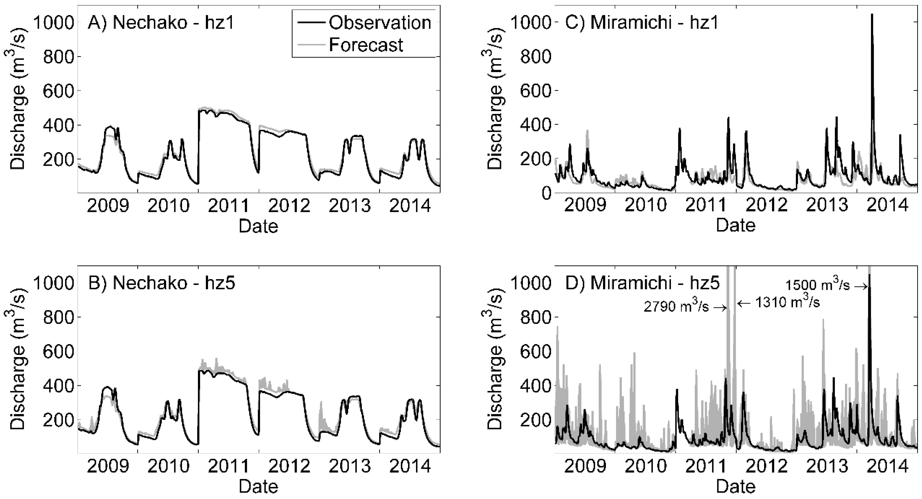
Figure 5.
Figure 5. MCRPS for: (A) discharge forecasts; (B) water temperature forecasts; and (C) Brier scores for both sets of forecasts. Brier Scores are represented for early warnings (EW) and threshold exceedance (TH).
Figure 5.
Figure 5. MCRPS for: (A) discharge forecasts; (B) water temperature forecasts; and (C) Brier scores for both sets of forecasts. Brier Scores are represented for early warnings (EW) and threshold exceedance (TH).

Figure 6.
Ensemble water temperature forecasts for a: (A) one-day lead time on the Nechako; (B) five-day lead time on the Nechako; (C) one-day lead time on the Miramichi; and (D) five-day lead time on the Miramichi.
Figure 6.
Ensemble water temperature forecasts for a: (A) one-day lead time on the Nechako; (B) five-day lead time on the Nechako; (C) one-day lead time on the Miramichi; and (D) five-day lead time on the Miramichi.

Figure 7.
Ensemble spreads of water temperature forecasts for lead times of one to five days on the Nechako (grey line) and the Miramichi (black line).
Figure 7.
Ensemble spreads of water temperature forecasts for lead times of one to five days on the Nechako (grey line) and the Miramichi (black line).
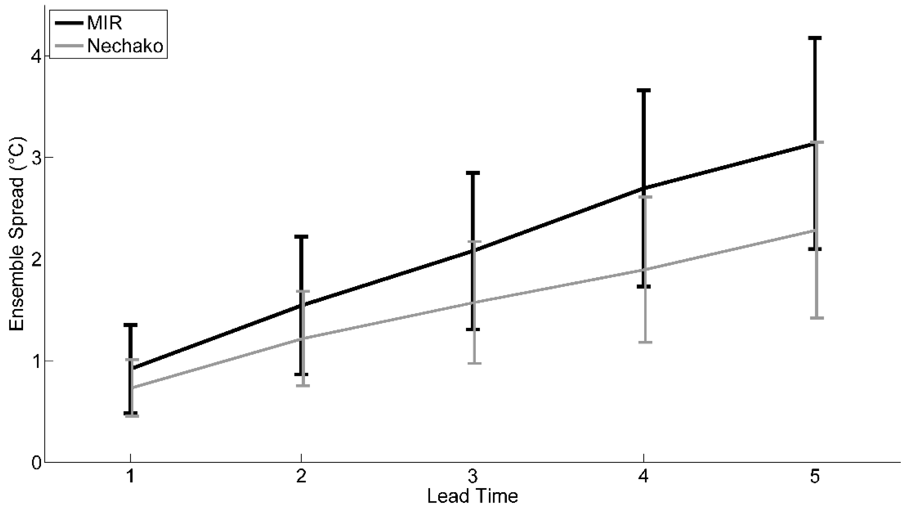
Figure 8.
Reliability plots for discharge ensemble forecasts on: (A) the Nechako; and (B) the Miramichi.
Figure 8.
Reliability plots for discharge ensemble forecasts on: (A) the Nechako; and (B) the Miramichi.

Figure 9.
Reliability plots for water temperature ensemble forecasts on: (A) the Nechako; and (B) the Miramichi.
Figure 9.
Reliability plots for water temperature ensemble forecasts on: (A) the Nechako; and (B) the Miramichi.

Table 1.
Calibration results for the hydrological and the thermal model on the Nechako (NECH) and Miramichi (MIR) watersheds.
Table 1.
Calibration results for the hydrological and the thermal model on the Nechako (NECH) and Miramichi (MIR) watersheds.
| Discharge | Water Temperature | |||||||||||||
|---|---|---|---|---|---|---|---|---|---|---|---|---|---|---|
| Year-Round | Summer | |||||||||||||
| NS | Bias (m3/s) | Relative Bias | RMSE (°C) | Bias (°C) | RMSE (°C) | Bias (°C) | ||||||||
| Period | NECH | MIR | NECH | MIR | NECH | MIR | NECH | MIR | NECH | MIR | NECH | MIR | NECH | MIR |
| Calibration | 0.96 | 0.84 | 8.87 | −3.03 | 0.12 | 0.01 | 1.38 | 1.37 | 0.24 | −0.54 | 0.78 | 1.23 | 0.43 | −0.76 |
| Validation | 0.86 | 0.72 | −10.4 | −18.6 | 0.13 | 0.13 | 1.54 | 1.51 | 0.2 | 0.09 | 0.95 | 1.46 | 0.37 | 0.18 |
Table 2.
MCRPS between ensemble forecasts and observations for all meteorological variables on the Nechako and on the Miramichi.
Table 2.
MCRPS between ensemble forecasts and observations for all meteorological variables on the Nechako and on the Miramichi.
| Hz1 | Hz2 | Hz3 | Hz4 | Hz5 | ||||||
|---|---|---|---|---|---|---|---|---|---|---|
| NECH | MIR | NECH | MIR | NECH | MIR | NECH | MIR | NECH | MIR | |
| tmin (°C) | 3.30 | 1.97 | 3.50 | 2.14 | 3.70 | 2.25 | 3.70 | 2.26 | 3.80 | 2.47 |
| tmax (°C) | 1.60 | 1.35 | 1.50 | 1.42 | 1.60 | 1.53 | 1.60 | 1.66 | 1.80 | 1.81 |
| pTot (mm) | 0.70 | 2.03 | 1.00 | 2.18 | 1.60 | 2.04 | 2.00 | 2.87 | 2.80 | 3.00 |
| RS (MJ/m2) | 2.50 | 2.32 | 2.50 | 2.40 | 2.50 | 2.76 | 2.70 | 3.75 | 3.10 | 3.25 |
| CC (0–1) | 0.15 | 0.16 | 0.14 | 0.16 | 0.14 | 0.17 | 0.14 | 0.18 | 0.15 | 0.19 |
| U (km/h) | 1.35 | 2.13 | 1.36 | 2.05 | 1.34 | 2.07 | 1.29 | 2.18 | 1.55 | 2.16 |
| ea (mm Hg) | 3.17 | 1.24 | 3.10 | 1.19 | 3.04 | 1.19 | 2.96 | 1.22 | 3.06 | 1.28 |
Table 3.
Forecasts previously produced on the Nechako and on the Little Southwest Miramichi River (LSWM) on the Miramichi watersheds.
Table 3.
Forecasts previously produced on the Nechako and on the Little Southwest Miramichi River (LSWM) on the Miramichi watersheds.
| Nechako | |||||
| Hz1 | Hz2 | Hz3 | Hz4 | Hz5 | |
| MAE (°C) | 0.49 | 0.58 | 0.55 | 0.54 | 0.68 |
| Miramichi (LSWM) * | |||||
| Hz1 | Hz2 | Hz3 | Hz4 | Hz5 | |
| RMSE (°C) | 0.87 | 1.24 | 1.48 | - | - |
| Bias | −0.01 | −0.03 | −0.03 | - | - |
* Caissie et al. [56].
© 2017 by the authors. Licensee MDPI, Basel, Switzerland. This article is an open access article distributed under the terms and conditions of the Creative Commons Attribution (CC BY) license (http://creativecommons.org/licenses/by/4.0/).
Share and Cite
MDPI and ACS Style
Ouellet-Proulx, S.; St-Hilaire, A.; Boucher, M.-A. Water Temperature Ensemble Forecasts: Implementation Using the CEQUEAU Model on Two Contrasted River Systems. Water 2017, 9, 457. https://doi.org/10.3390/w9070457
AMA Style
Ouellet-Proulx S, St-Hilaire A, Boucher M-A. Water Temperature Ensemble Forecasts: Implementation Using the CEQUEAU Model on Two Contrasted River Systems. Water. 2017; 9(7):457. https://doi.org/10.3390/w9070457
Chicago/Turabian StyleOuellet-Proulx, Sébastien, André St-Hilaire, and Marie-Amélie Boucher. 2017. "Water Temperature Ensemble Forecasts: Implementation Using the CEQUEAU Model on Two Contrasted River Systems" Water 9, no. 7: 457. https://doi.org/10.3390/w9070457
Note that from the first issue of 2016, this journal uses article numbers instead of page numbers. See further details here.