An Assessment of Mean Areal Precipitation Methods on Simulated Stream Flow: A SWAT Model Performance Assessment


1
Department of Forestry, Water Resources Program, School of Natural Resources, University of Missouri, 203-T ABNR Building, Columbia, MO 65211, USA
2
Davis College, Schools of Agriculture and Food, and Natural Resources, West Virginia University, 3109 Agricultural Sciences Building, Morgantown, West Virginia 26506, USA
3
Institute of Water Security and Science, West Virginia University, Morgantown, WV, USA
*
Author to whom correspondence should be addressed.
Water 2017, 9(7), 459; https://doi.org/10.3390/w9070459
Submission received: 2 April 2017
/
Revised: 17 June 2017
/
Accepted: 21 June 2017
/
Published: 24 June 2017
Abstract
:Accurate mean areal precipitation (MAP) estimates are essential input forcings for hydrologic models. However, the selection of the most accurate method to estimate MAP can be daunting because there are numerous methods to choose from (e.g., proximate gauge, direct weighted average, surface-fitting, and remotely sensed methods). Multiple methods (n = 19) were used to estimate MAP with precipitation data from 11 distributed monitoring sites, and 4 remotely sensed data sets. Each method was validated against the hydrologic model simulated stream flow using the Soil and Water Assessment Tool (SWAT). SWAT was validated using a split-site method and the observed stream flow data from five nested-scale gauging sites in a mixed-land-use watershed of the central USA. Cross-validation results showed the error associated with surface-fitting and remotely sensed methods ranging from −4.5% to −5.1%, and −9.8% to −14.7%, respectively. Split-site validation results showed the percent bias (PBIAS) values that ranged from −4.5% to −160%. Second order polynomial functions especially overestimated precipitation and subsequent stream flow simulations (PBIAS = −160) in the headwaters. The results indicated that using an inverse-distance weighted, linear polynomial interpolation or multiquadric function method to estimate MAP may improve SWAT model simulations. Collectively, the results highlight the importance of spatially distributed observed hydroclimate data for precipitation and subsequent steam flow estimations. The MAP methods demonstrated in the current work can be used to reduce hydrologic model uncertainty caused by watershed physiographic differences.
1. Introduction
Accurate mean areal precipitation (MAP) estimates are essential forcing data for hydrologic models [1,2]. However, quantifying MAP can be confounding, particularly when metrological conditions, topography, and/or land use influence the spatiotemporal variability of precipitation [3]. There are multiple techniques that have been used to estimate MAP including (but not limited to) nearest neighbor (or proximate gauge), direct weighted average, surface-fitting, and remote sensing (e.g., radar and satellite-based) methods. Selecting the most suitable method to estimate MAP can be daunting, in part, because there are so many methods to choose from, each with distinct strengths and weaknesses.
Studies have shown a correlation between gauge density and the accuracy of MAP estimates [4]. In regions without observed data, MAP can be simulated using statistical weather generators. However, remotely sensed data may be more accurate in ungauged watersheds [5]. In minimally gauged regions, where at least one gauge is available, the proximate gauge method can be used to estimate MAP. Using this method, MAP is assumed to be equal to the total rainfall from the gauge nearest to the centroid of a given sub-basin [6]. However, uncertainty increases with the distance from the point of measurement making this approach problematic for many applications [4]. Model uncertainty can be reduced by increasing the gauge density [4]. In regions with more than one gauge, precipitation data can be interpolated to estimate MAP using direct weighted averaging methods, or surface-fitting methods. Some examples of direct weighted averaging methods include arithmetic average, Thiessen polygons [7], and the two-axis method [8]. Popular surface-fitting methods include polynomial surface [9], spline surface [9], inverse-distance interpolation (IDW) [10], multiquadric interpolation [9], optimal interpolation/kriging [11], artificial neural networks [12,13,14], and hypsometric methods [15].
While there are many MAP methods, choosing the appropriate method for a given application is critical. For example, a relatively simple arithmetic average may be appropriate for a spatially lumped hydrologic modeling application in a small watershed of relatively homogenous topography and land use, but a more computationally complex hypsometric method (for example: The Parameter-elevation Regression on Independent Slopes Model (PRISM)) may be well-suited for a spatially distributed hydrologic modeling application in a mountainous region [15,16]. Furthermore, an inverse-distance interpolation method may be a more appropriate approach for a physically-based semi-distributed model such as the Soil and Water Assessment Tool (SWAT) [17].
Similar to the MAP method selection, it is also important to select the most appropriate hydrologic simulation model for the application. While there are multiple hydrologic models to choose from, SWAT is currently one of the most popular hydrologic models world-wide with over 2500 publications in print in over 400 different scientific journals [18]. The SWAT model is used internationally for applications including water resource management, pollutant loading estimates, receiving water quality, source load allocation determinations, and conservation practice efficacy [5,19]. A complete description of the SWAT model can be found in the Soil and Water Assessment Tool Theoretical Documentation [6], and literature reviews highlight various strengths and weaknesses of the model [5,19,20]. A SWAT Literature Database can be accessed via the internet at (http://swat.tamu.edu/publications/swat-literature-database).
While there are numerous SWAT modeling publications, there are relatively few publications on the topic of precipitation input effects on the SWAT model output. However, the effects of different precipitation inputs on the SWAT model output have been tested using remotely sensed data [21,22,23,24,25] and the centroid method currently used to estimate MAP in SWAT [4,17,21,22,23,24,26,27]. For example, Tuo et al. [26] tested the influence of the centroid method, IDW, and two satellite-based data sets (the Tropical Rainfall Measuring Mission (TRMM), and Climate Hazards Group InfraRed Precipitation with Station data (CHIRPS)) on SWAT simulated stream flow in the alpine Aldige river basin of north-eastern Italy. Results showed that the IDW method was the most accurate method tested for SWAT model precipitation input, and the CHIRPS satellite-based data set produced ‘satisfactory’ simulations of stream flow. Szczesniak and Pinieski [17] used four methods including the nearest neighbor technique, Thiessen polygons, IDW, and ordinary kriging (OK) in the Sulejów Reservoir Catchment located in Poland. The results showed the OK method as the most accurate interpolation method for the SWAT model. Additionally, the OK, IDW, and Thiessen methods were more accurate than the centroid method, currently the default method, used in SWAT with median differences in Nash-Sutcliffe values ranging from 0.05 to 0.15. Masih et al. [4] tested the IDW method versus the default method used in SWAT in mountainous semiarid catchments in the Karkheh River basin, Iran. The IDW method resulted in an improved SWAT model output particularly in smaller watersheds with drainage areas ranging from 600 to 1600 km2. Ultimately, the results from the literature consistently show that the centroid method currently used in SWAT is unsatisfactory for most applications.
Many methods used to estimate MAP have been reviewed in cross-validation studies [28,29,30,31]. Generally, the results showed that more complicated surface-fitting methods generate better results relative to direct weighted averaging methods. However, the computational demands of the more complex surface-fitting methods can be a disadvantage. A less frequently applied alternative approach to cross-validation analysis of MAP models is to validate the models against a hydrologic model simulated stream flow [17]. There remains a great need for a hydrologic model validation of multiple MAP methods across the array of contemporary MAP modeling techniques (i.e., proximate gauge, direct weighted average, surface-fitting, and remotely sensed methods). In addition, Masih et al. [4] and Ly et al. [27] concluded that there is a need for further testing of the effects of precipitation input on the SWAT model output.
In response to the call for further investigation, a novel split-site validation of multiple MAP techniques (e.g., proximate gauge, direct weighted average, surface-fitting, and remotely sensed methods) is presented using observed precipitation and stream flow data collected at nested-scales in a mixed-land-use catchment. The overarching purpose of the current work was to show which MAP method(s) are best-suited for hydrologic simulation modeling efforts so that managers can more readily focus on viable efforts in other developing watersheds with similar physiographic characteristics as the study catchment. The objectives of the current work were to: (i) quantify the effects of 19 different MAP methods on uncalibrated SWAT model performance for stream flow, and (ii) perform a split-site validation of SWAT model simulated stream flow using multiple years of observed stream flow data collected at nested-scales from a mixed-land-use watershed of the central USA.
2. Materials and Methods
2.1. Site Description
The study catchment, Hinkson Creek Watershed (HCW), is a rapidly urbanizing mixed-land-use (forest, agriculture, and urban) watershed located in Boone County, Missouri, USA (Figure 1). HCW has a total drainage area of approximately 230 km2. Elevation ranges from 274 m above mean sea level (AMSL) in the headwaters to 177 m AMSL near the watershed outlet. The climate in HCW is dominated by continental polar air masses in the winter and maritime and continental tropical air masses in the summer [32]. The wet season occurs primarily during March through June [33]. A 16-year climate record (2000–2015) obtained from the Sanborn Field climate station located on the University of Missouri campus showed that the mean annual total precipitation was 1036 mm, and the mean annual air temperature was 13.3 °C, respectively. Daily minimum and maximum air temperatures ranged from −23.1 °C in the winter to 41.3 °C in the summer.
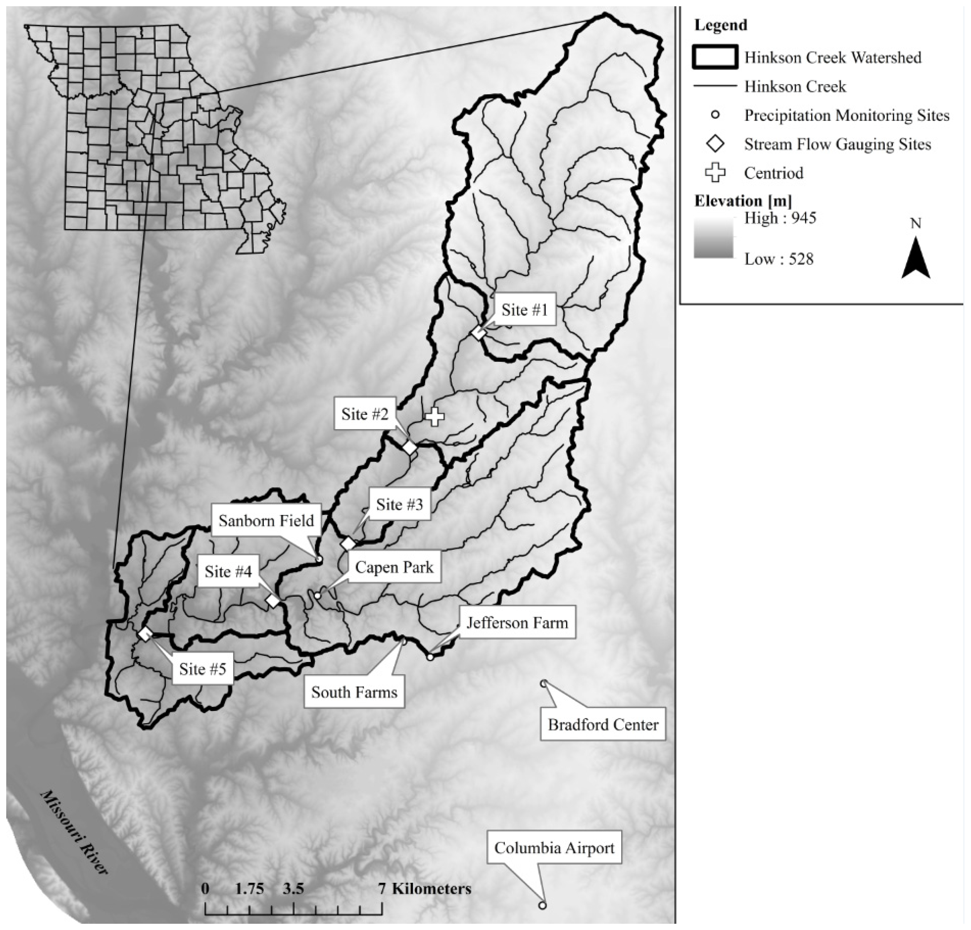
The HCW was instrumented with hydroclimate (n = 5) and meteorological (n = 6) monitoring sites in 2009. Precipitation was sensed using TE525WS tipping bucket rain gauges with an accuracy of +1% at 2.5 cm/h rainfall rate to −3.5% at 5.1 to 7.6 cm/h rainfall rate during the study period [water year’s (WY’s) 2009 to 2015]. A total of eleven precipitation monitoring sites were used for the current work including five Hinkson Creek hydroclimate sites (noted above), and six additional meteorological sites (The Columbia Regional Airport, and the five Missouri Agricultural Experimental sites) located in Boone County, Missouri, USA (Table 1, Figure 1). Site #1 was the sub-basin with the lowest precipitation gauge density. However, the precipitation gauge at the outlet was less than 14 km from the furthest ridge of the sub-basin at Site #1, thus resulting in a relatively high-resolution spatial sampling design. The five HCW hydroclimate sites were positioned to partition the study catchment into five sub-basins using a nested-scale experimental watershed study design each with different dominate land use types [32,34]. At the time of this research, agricultural land use decreased by 18.4% and urban land use increased by 21.6% with the downstream distance from Site #1 located in the headwaters to Site #5 located near the watershed outlet.
The stage was measured at each Hinkson Creek gauging site using Sutron Accubar® constant flow bubblers with an accuracy of 0.02% at 0–7.6 m to 0.05% at 7.6–15.4 m [35,36,37,38]. Precipitation and stage data were stored on Campbell Scientific CR-1000 data loggers. Methods used to estimate the discharge met the U.S. Geological Survey (USGS) standards [39]. The stream flow was measured using FLO-MATE™ Marsh McBirney flow meters and wading rods when the stage was less than 1-m deep. Storm flows were measured using a U.S. Geological Survey Bridge Board™. Stage-discharge rating curves were generated using the incremental cross section method [40].
2.2. MAP Modeling
Errors in precipitation estimates occur at the point measurement of precipitation (e.g., precipitation gauge), and during conversion of the point measurements to MAP. Error in precipitation measurement at a gauge may be caused by various factors including, but not limited to, wind, splash, evaporation, mechanical failure, improper instrument calibration, a plugged gauge orifice, isolated objects (e.g., trees, buildings, and fences), observation errors, and other factors [41,42]. Because point measurement is fraught with complications, it is important to examine the quality of precipitation data before undertaking hydrologic analyses [41,42]. Therefore, double-mass plots were created to check for undercatch due to obstructions at each gauging site where the precipitation was measured [43]. The results from the double-mass curve analyses indicated undercatch precipitation at Site #1 presumably attributable to a tree line induced fetch issue. The precipitation gauge at Site #1 was moved away from the tree line to approximately 250 meters south east of Site #1 on 16 June 2011. The undercatch issue was corrected as per methods used by Wagner et al. [44], where a calculated percentage was added to the time series recorded at Site #1 before the site was moved (Site #1 was installed on 1 February 2009). Additionally, any missing precipitation data (i.e., data gaps) were estimated using inverse distance weighting methods [45].
After rainfall data post-processing, 19 different methods were used to estimate MAP for each sub-basin in HCW including two proximate gauge methods, three direct weighted average methods, ten surface-fitting methods, and three satellite-based methods (Table 2). The MAP methods chosen for this assessment ranged from simplistic to complex in order to address the needed balance between computational complexity and the ease of use. Nineteen MAP methods were included in the analysis to avoid erroneous selection of the most convenient method while at the same time providing a comprehensive overview (and validation) of many of the different types of methods available.
2.2.1. Proximate Gauge MAP Methods
The proximate gauge MAP models (i.e., Centroid and Outlet) were the simplest methods and were dependent on the fewest number of precipitation gauges. For example, the centroid method used data from three precipitation gauges (Sites #1, #2, and #4), and the outlet method used data from five precipitation gauges. For the centroid method, MAP was estimated as the precipitation measured at the precipitation gauge nearest the centroid of a sub-basin. For the outlet method, MAP was estimated as the precipitation measured at the outlet of each sub-basin (Sites #1, #2, #3, #4, and #5).
2.2.2. Direct-Weighted Average Methods
Direct weighted averages are computationally simplistic methods used to generate estimates of MAP with the following general equation [31]:
where MAP is mean areal precipitation for G gauges termed g = 1, g = 2, …, G, pg is the precipitation measured at each gauge, and wg are the weights based on the sub-basin area that satisfy:
The coefficients for each of the direct weighted averaging models were fit using ArcGIS.
The arithmetic average is the simplest direct weighted averaging method. Each gauge has an equal weight in the computation of a single arithmetic average for the entire watershed. The equation used to calculate the arithmetic average follows [31]:
The arithmetic average method is useful in estimating missing precipitation data using data collected from nearby gauging stations. However, this method does not represent the spatial variability observed in the precipitation data.
The Thiessen method is a direct weighted average method performed by dividing a region into sub-regions centered on each monitoring site [7]. Each sub-basin does not line up with the Thiessen sub-region. However, the fraction of each Thiessen sub-region contributing to each sub-basin can be computed, and weighted averages can be used to estimate MAP for each sub-basin. The equations used to compute the spatial average follow:
where ag is the area of each sub-region.
Bethlahmy [8] developed the two-axis method where weights are derived using basic geometry. The two-axes include a major axis and a minor axis. First, three lines are drawn, (1) the longest line that can be drawn in the region, (2) its perpendicular bisector (the minor axis), and (3) is the perpendicular bisector of the minor axis (the major axis). Then, two lines are drawn from each gauge to the furthest end of each axis, and the angle of the two lines is recorded. Finally, the equations used to calculate MAP are as follows:
where Å is the sum of all of the angles αg.
2.2.3. Surface-Fitting MAP Methods
Surface-fitting algorithms were also used to generate MAP from point gauges using the ArcGIS software. The general equations used to calculate the weighted averages for each cell are as follows [42]:
where wjg are weights for each cell, pj is precipitation value for each cell, and J is the total number of all cells. The difference between various surface-fitting methods used is how the weights are calculated.
Surface fitting algorithms can be classified as deterministic or statistical methods. Global polynomial surface (GPS) and local polynomial surface (LPS) functions are deterministic methods commonly used to interpolate rainfall [9]. All point measurements are considered when using the GPS method. Conversely, only point measurements within a defined radius are considered with the LPS method. For both GPS and LPS methods, the order of the polynomial function must be defined by the end user. A linear plane results from a 1st order polynomial, one turning point (i.e., curve) results in a surface generated by a 2nd order polynomial, two curves are present for the 3rd order polynomial, and so on. Unlike the GPI and LPI methods, Radial Basis Functions (RBFs) are an exact interpolator. Some examples of RBFs include spline and multiquadric interpolation. RBFs generate a smooth surface and the degree of smoothness is dependent on the kernel parameter [9]. Conversely, IDW is an inexact interpolator. Thus, unlike RBFs, IDW fitted-surfaces may not be exactly equal to the point measurements used to generate the surface. The assumption behind the method of IDW is that each unknown point in the surface is more alike its closest neighboring point measurement [10]. The equations used to calculate IDW is [31]:
where dpj is distance from point j to the gauge, and −m was an exponent assigned by the end user.
Kriging is a statistical surface-fitting method where the weights to each cell minimize the variance of the interpolation error [11]. Empirical semivarience is computed using input data and a curve is fit to develop a semivariogram. Then, predictions are made for each cell using kriging weights generated from the semivariogram [31]. Some examples of kriging methods include ordinary kriging (OK) and universal kriging (UK). The OK method generates a smooth surface, minimizes the standard error, but no spatial trend in precipitation is accounted for. Conversely, the UK method can be used to account for the presence of a spatial trend or drift.
The surface-fitting methods were applied using the ArcGIS ‘model builder’ to efficiently interpolate observed point measured precipitation data into MAP for each HCW sub-basin (n = 5). A split-site method was used to calibrate and validate the surface-fitting models and remotely sensed data against point gauge measured precipitation. Sites #1–5, Capen Park, Bradford Center, and Columbia Regional Airport were used for calibration. Sanborn Field, South Farm, and Jefferson Farm monitoring sites were used for validation. Three model performance criteria were used to evaluate the model performance including percent bias (PBIAS), root mean square error (RMSE), and mean absolute error (MAE) [35,46,47].
2.2.4. Remotely-Sensed MAP Methods
MAP was also estimated using three satellite-based datasets. The three satellite-based precipitation data included PRISM, TRMM, and CHIRPS data. The PRISM data were downloaded from an Oregon State University website [48]. Daily precipitation data grids (4 km raster images) corresponding to the ‘AN81d’ data set were downloaded one year at a time in the .bil format. Area-averaged TRMM Multi-Satellite Precipitation Analysis (3b42) data were downloaded at a daily time step from the Giovanni website [49]. Area-averaged CHIRPS data were downloaded at a daily time step from the ClimateServ website for this research [50]. Additionally, MAP was estimated using a level III daily precipitation product of Next Generation Radar Data (NEXRAD) which were bulk downloaded from a National Weather Service File Transfer Protocol server [51].
Models were created in ArcGIS using the ‘model builder’ to extract precipitation data from each surface raster file to each precipitation monitoring site (n = 11) for validation. Three model performance criteria were used to evaluate the model performance including PBIAS, RMSE, and MAE [35,46,47]. Sanborn Field, South Farm, and Jefferson Farm monitoring sites were used for validation.
2.3. SWAT Modeling
After MAP was generated and the MAP models were validated, the model output was formatted for input into SWAT (SWAT 2012 (Revision 627 packaged with ArcSWAT 2012.10_2.16)) to test the effects of the 19 different MAP methods on the uncalibrated SWAT model output of the stream flow. An uncalibrated model performance assessment was appropriate in the current work. This is justifiable considering that the SWAT model was designed to generate reliable predictions in ungauged basins [6]. These results are important for end users who rely on remotely-sensed precipitation data. A 30 m digital elevation model, SSURGO soils, and the 2011 National Land Cover Data sets were used for the spatial input data required to create a SWAT project. The SCS curve number method, the Muskingum method, and the Penman-Monteith method were selected to simulate rainfall-runoff, channel routing, and evapotranspiration processes, respectively. Channel degradation, stream water quality, and algae-biochemical oxygen demand-dissolved oxygen simulations were all set to ‘active’. Calibration parameters were set to reflect physically realistic values for the watershed [52]. Agricultural HRU’s were set to a corn-soybean rotation with three fertilization operations (anhydrous ammonia, elemental nitrogen, and elemental phosphorus) and tandem disk tillage in the spring. Grazing pasture HRU’s were set to hay growing operations, fertilizer operations (elemental nitrogen, and elemental phosphorus), and grazing operations realistic for HCW. Urban HRU’s were set to a tall fescue growing operation with lawn fertilization and street sweeping operations. Water abstractions were not implemented in the SWAT model.
For each SWAT project (n = 19, one for every MAP method tested), the precipitation text files were updated from the “txt in out” folder under the “default” scenario. The uncalibrated SWAT model output was tested to isolate only the effects of the precipitation input on SWAT simulated stream flow. Additionally, the SWAT model was calibrated using the auto-calibration software SWAT-cup and validated using a split-site method for stream flow at daily, monthly, and annual time steps [5,52]. Site #4 (the HCW USGS operated gauge) was used for calibration. Sites #1, #2, #3, and #5 were reserved for validation.
In the current work, one global sensitivity analysis was applied using SWAT-cup as per methods used by Szczesniak and Pinieski [4] and Masih et al. [17]. A global sensitivity analysis was run using SWAT’s default method for precipitation input (centroid method) and the top six most sensitive calibration parameters were selected for the calibration of all MAP models. The six calibration parameters selected included the Soil Conservation Service (SCS) curve number (CN2), surface runoff lag time (SURLAG), available water capacity of the soil (SOL_AWC), manning’s n value for overland flow (OV_N), base flow alpha factor (ALPHA_BF), and groundwater delay (GW_DELAY). User-specified physically meaningful minimum and maximum bounds were set for CN2 (absolute −5 to 5), SURLAG (replace 1 to 7), SOL_AWC (absolute −0.05 to 0.05), OV_N (absolute −0.09 to 0.25), ALPHA_BF (replace 0.3 to 0.8), and GW_DELAY (replace 10 to 200), where ‘absolute’ indicates the addition of the given value to the existing value and ‘replace’ indicates the replacement of the existing value with the given value. Four iterations of 250 simulations (i.e., a total of 1000 simulations) each were run for each of the 19 different MAP methods. The model was calibrated at a daily time step. Seven years of stream flow data were simulated (January 2008 to December 2014) with an additional seven years to warm-up the model (2001 to 2008). Model outputs were reduced by averaging to the monthly and annual time steps for analysis because daily simulations are typically poorer than monthly and annual simulations [47,53]. Uncalibrated and calibrated model performances were assessed using three model evaluation criteria for NSE, R2, and PBIAS, shown in Table 3 [52]. Each MAP method was ranked by model performance values (PBIAS, NSE, and R2) at each time interval (daily, monthly, and annual) for easy comparison. Then, a relative overall model performance rank was quantified by summing the ranks of the individual model performance values across all time intervals.
3. Results and Discussion
3.1. MAP Modeling
When the observed precipitation from all eleven monitoring sites were averaged, the results showed that the average annual total precipitation ranged from 743 mm during water year (WY) 2012 to 1543 mm during WY 2010 (Table 4). The observed precipitation at Sanborn Field and South Farm was within 6 mm of the all-site mean, but the precipitation at Jefferson Farm was 67 mm less than the seven-year mean. Double-mass curve analyses did not indicate precipitation undercatch due to gauge obstructions at the validation sites, thus the differences in annual total precipitation were presumably due to spatial variability of precipitation during the study period.
The results from the one-way ANOVA tests showed no significant differences (p > 0.05) in the seven-year average precipitation between sites in agreement with a recent publication by Hubbart et al. [33]. Hubbart et al. [33] showed that the differences in precipitation between urban and rural sites were not significant at the 95% confidence level in the HCW. However, precipitation was shown to be slightly greater by 3.3% in the urban area of the watershed indicating a slight influence of urban land use on total annual precipitation in the rapidly urbanizing lower elevations of HCW [38].
The results showed that the seven-year average annual total MAP estimates ranged from 1019 mm (Thiessen) to 1192 mm (NEXRAD) (Table 5). There were significant differences (p < 0.001) in the five-site average MAP between years. This was expected considering the occurrence of extremely wet and dry years during the study (Table 5). Conversely, there were no significant differences (p > 0.05) in the seven-year average MAP between sites.
When surface-fitting methods and remote sensing methods were validated, the results showed that the models consistently overestimated the annual total precipitation (Table 6). Results from one-way ANOVA tests showed that the seven-year average MAP was significantly (p < 0.01) greater by a range of 5.9% to 15.7% for all four remotely sensed methods relative to all other methods tested. This was an important finding from the current work with implications for end-users that need to use remotely-sensed precipitation data for hydrologic modeling efforts. However, there were no significant differences (p > 0.05) in the seven-year average MAP between proximate gauge, direct-weighted average, and surface-fitting methods.
The lack of significant differences between annual average MAP estimated by proximate gauge, direct-weighted average, and surface fitting methods was surprising in the current work, and unanticipated. It was further surprising considering that the findings from other studies showed improvements in hydrological output with computational complexity and gauge density [4,17]. For example, there were differences in the equations for each MAP method (n = 19 methods) ranging across a simple-complex gradient of computational rigor. Also notable were the marked differences in gauge density between the centroid method (n = 3 gauges), the outlet method (n = 5 gauges), and direct weighted averaging and surface-fitting methods (n = 11 gauges). The lack of statistical differences was counter to the literature, and thus should be of interest, considering differences in climate and physiography between the study sites.
Validation results showed variable results for maximum daily MAP estimates. For example, maximum daily MAP was underestimated by greater than 50% for two remote sensing methods (i.e., CHIRPS and PRISM), and two direct weighted average methods (i.e., Average and Two-Axis). Conversely, maximum daily MAP was overestimated by more than 160% for the 2nd order polynomial functions (i.e., GPI_2 and LPI_2). The 2nd order polynomial functions generated unrealistic estimates of the daily maximum MAP because the model output increased with the distance upslope of Site #1. Conversely, the 1st order polynomial functions were within 16% of the observed maximum daily MAP. Thus, in the current work, the linear polynomial functions were more accurate than the nonlinear order polynomial functions. Polynomial functions of cubic or greater order that result in a surface with multiple turning points (i.e., a rippled or wavy surface) were not tested.
3.2. SWAT Modeling
3.2.1. Uncalibrated Model Performance
In comparison to previous work, this study is the first to show the effects of MAP input on uncalibrated SWAT stream flow at daily, monthly, and annual time steps. Considering that the model calibration influences the model output, the uncalibrated results completely isolated the effects of precipitation input on the SWAT model performance. There was a general trend for uncalibrated model performance to increase as the stream flow data were reduced by averaging from daily to annual time steps. For example, uncalibrated daily SWAT model performance ratings for stream flow were ‘unsatisfactory’ for every MAP method tested due to low NSE and R2 values (Table 7). As the streamflow data were reduced by averaging from a daily to monthly time step, NSE and R2 values increased leading to model performance that ranged from ‘unsatisfactory’ to ‘satisfactory’. SWAT model simulations of annual stream flow ranged from ‘unsatisfactory’ to ‘good’.
Overall model performance ratings were more limited by NSE and R2 values at daily timesteps and by PBIAS at annual timesteps. For example, the results showed that the NSE and R2 values improved by an average of 0.60 and 0.47, respectively, as the stream flow data were reduced by averaging from daily to annual time steps, while the PBIAS ratings were nearly equal for daily, monthly, and annual time steps. These results indicated that one threshold for PBIAS is appropriate for all timesteps (e.g., daily, monthly, and annual) in agreement with the model performance criteria recently published by Moriasi et al. [46], and point to the potential benefit of considering different NSE and R2 thresholds for each timestep.
Notably, some MAP methods resulted in ‘unsatisfactory’ model performance across all time scales reflected in the PBIAS values ±15% even when the NSE and R2 values were adequate. There may be a need to reconsider changing the PBIAS threshold to ±25% as proposed by Moriasi et al. [47] to better capture adequate model performance at monthly and annual timesteps. These results also highlighted a problem with the threshold dependent overall model performance rating criteria when selecting the best MAP method. The problem was resolved by ranking the model performance output to highlight the best MAP method tested.
When the uncalibrated SWAT model performance values were ranked, the results showed that the remotely sensed PRISM data set performed best overall (i.e., all time steps tested considered) (Table 7). The PRISM method resulted in the greatest NSE and R2 results at monthly and annual timesteps, indicating that the PRISM method was best-suited for long-term estimates of stream flow in the study catchment (Table 7). However, the results showed that the daily estimates of stream flow were ‘unsatisfactory’ for the uncalibrated models. These results are in general agreement with results provided by Srinivasan et al. [54] who used similar GIS-based methods to aggregate 4 km PRISM data for SWAT model precipitation input, and ran the model ungauged (i.e., uncalibrated) to show that the uncalibrated SWAT model can produce satisfactory estimates of hydrology at an annual time step in the Upper Missouri River Basin with PBIAS values within ±10%, and NSE values ranging from 0.51 to 0.95. Unlike the results from Srinivasan et al. [54], the model performance was also ‘satisfactory’ for the monthly stream flow in the current work, but only near the watershed outlet because the model did not simulate hydrology well in the agricultural dominated headwaters.
Examination of the model performance ratings at the validation sites (Sites #1, #2, #3, and #5) indicated that the uncalibrated SWAT model performance ratings were unsatisfactory at every time step at Sites #1 and #2 due to overestimation of the stream flow in the predominantly agricultural headwaters (e.g., PBIAS values less than −175%), likely (in part) due to clay pan soils characterized by increased surface runoff rates that the model simulations over-accounted for [55], considering that Baffaut et al. [55] reported on the complications of SWAT modeling applications in watersheds with clay pan soils in the central US. In the current work, the PBIAS values ranged from −51.0 (Two-Axis) to less than −163.0 (GPI_2, LPI_2) at Site #1 (Figure 2). Conversely, the stream flow was generally underestimated at Site #5 with PBIAS values greater than 15% for most of the MAP methods tested except for four MAP methods (i.e., GPI_2, LPI_2, PRISM, and NEXRAD). The stream flow at urban Site #5 was likely underestimated (at least in part) due to the impacts of increased impervious surfaces on the stream flow which the model did not simulate well.
3.2.2. Calibrated Model Performance
Model calibration improved the model performance at Site #4 (Table 8). The differences in fitted calibration parameter values for each MAP method are shown in Figure 3. When calibrated SWAT model performance was ranked, the IDW_2 method performed best overall (i.e., all time steps tested were considered) (Table 8). The IDW_2 method has also been shown to work well in other locations with considerably different climate and physiographic characteristics compared to the study catchment [4,17,26]. For example, Tuo et al. [26] showed that the IDW method was the most accurate method tested for SWAT model precipitation input on SWAT simulated stream flow in an alpine Aldige river basin of north-eastern Italy. Szczesniak and Pinieski (2015) showed that IDW was more accurate than the centroid method in the Sulejów reservoir catchment in central Poland. Masih et al. [4] successfully tested the IDW method versus mountainous semiarid catchments in the Karkheh River basin, Iran. Thus, the results show that IDW_2 is a robust interpolation method that can improve SWAT model performance in various regions globally.
The results from the current work and other studies showed mixed results from remotely sensed data. Tuo et al. [26] tested the influence of satellite-based data sets (TRMM and CHIRPS) on SWAT simulated stream flow. The CHIRPS data resulted in ‘satisfactory’ simulations of the stream flow [26]. However, the TRMM data set was associated with ‘unsatisfactory’ model performance by Tuo et al. [26]. In the current work, TRMM and CHIRPS data were ranked at 16th and 17th, respectively, indicating poor overall model performance relative to the other MAP methods tested. However, it is important to note that model calibration improved the model performance adequately at an annual timestep using the TRMM and CHIRPS input data in the current work.
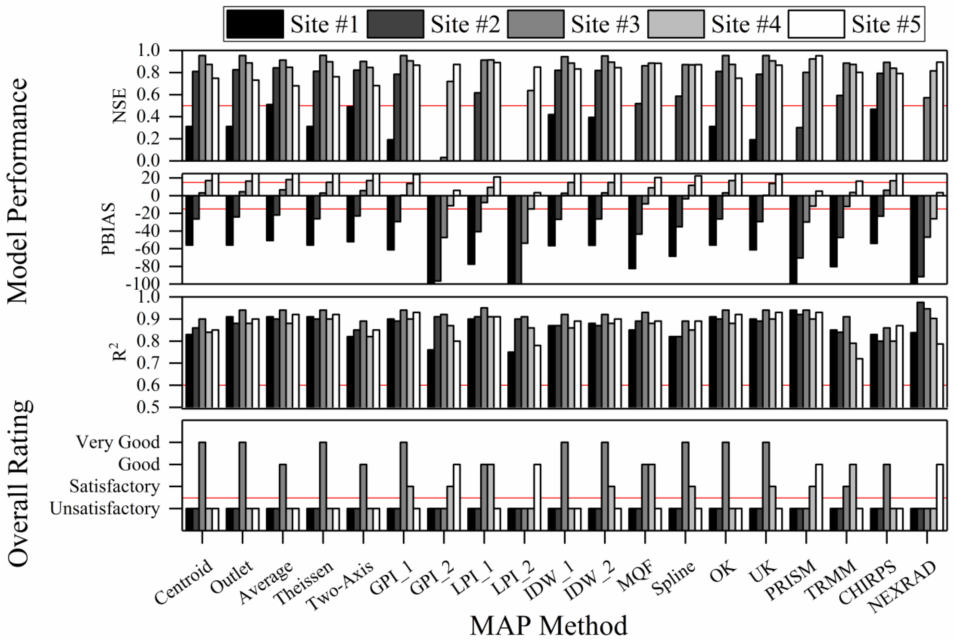
Examination of the model performance ratings at the validation sites (Sites #1, #2, #3, and #5) indicated that the PBIAS values decreased to less than −68% in the agricultural headwaters due to notable differences in soils, vegetation, land use, and underlying geology that the SWAT model did not simulate well (Figure 4). The study catchment was divided by two Level II Ecoregions [35]. The agricultural headwaters were within the Great Plains ecoregion while the urbanizing lower elevations were in the Ozark Highlands ecoregion. Thus, the split-site validation results indicated that calibrating the model at only the watershed outlet is not advised in watersheds with substantial changes in watershed physiographic characteristics. These results have implications for water resource management practices based on the SWAT model output in large basins (e.g., Upper Mississippi River Basin) that often contain multiple ecoregions coupled with differences in watershed characteristics.
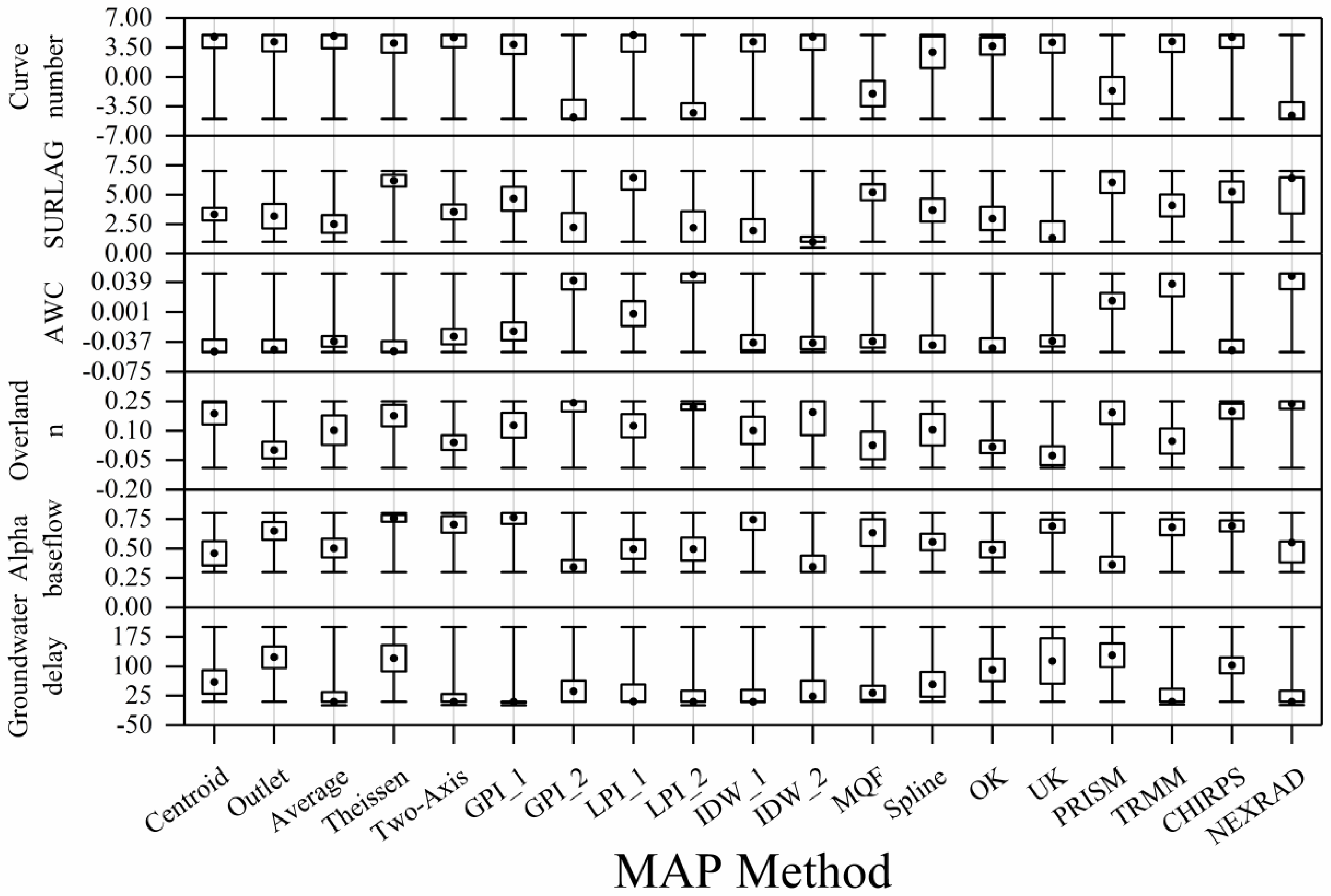
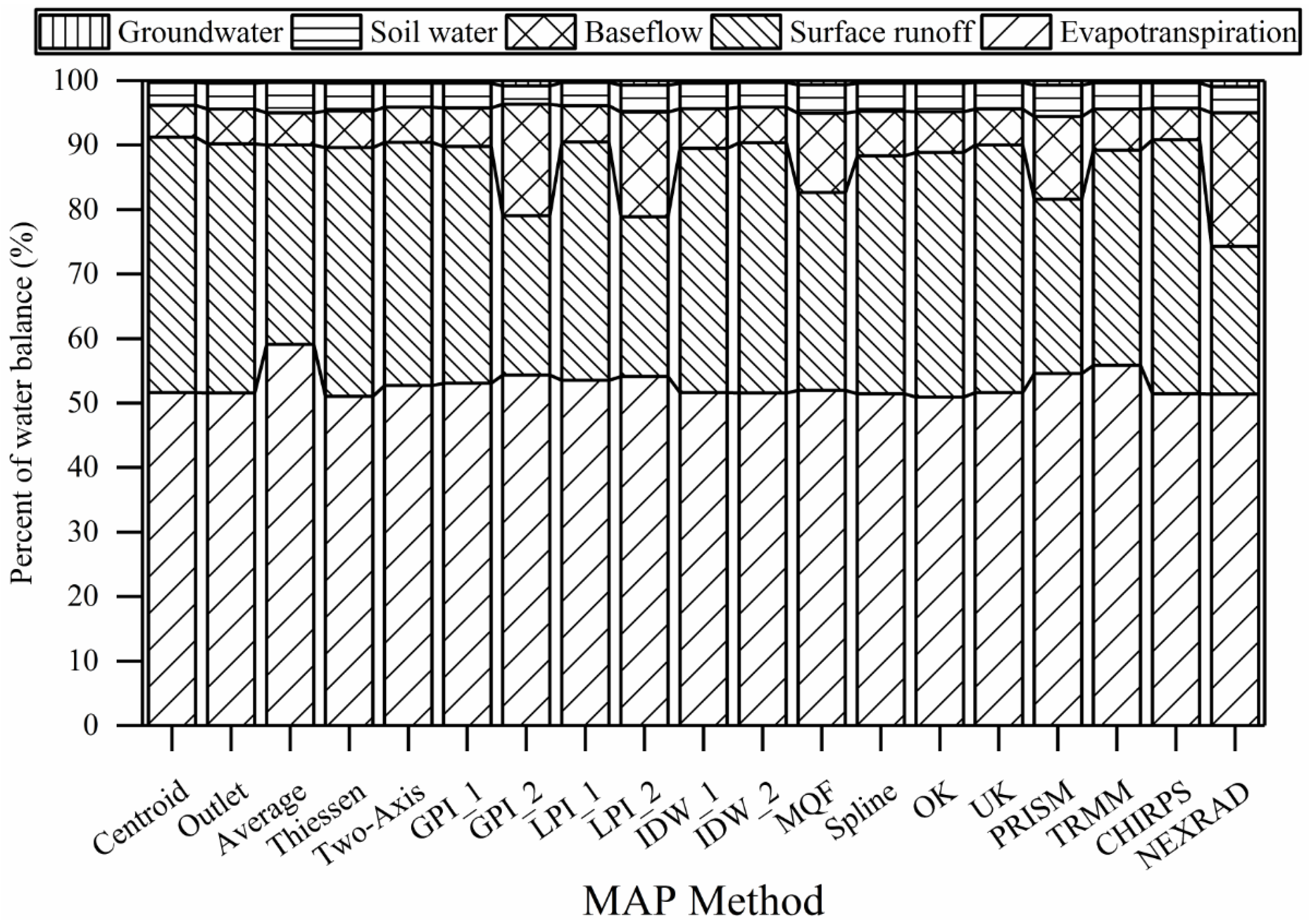
The MAP input data affected the SWAT model simulated water balance variables (Table 9, Figure 5). For example, ET and stream flow accounted for the majority of the water balance. However, the greatest differences in the water balance components were in the amount of total stream flow that was the base flow as shown in Figure 5. For example, the SWAT model simulated BFI’s ranged from 11% to 48% while the observed BFI was 25% for the study catchment [36]. BFI was overestimated when the MAP methods overestimated the annual total precipitation (GPI_2, LPI_2, PRISM, and NEXRAD). In the current work, to attenuate the overestimations of precipitation generated using the GPI_2, LPI_2, PRISM, and NEXRAD MAP methods, SWAT-cup autocalibration routines resulted in the greatest reductions of curve numbers (CN2-5) coupled with the greatest increases in overland roughness (OV_N+0.25) and available water capacity of the soil (SOL_AWC+0.05) (Figure 3). The combined effects of minimizing the curve numbers, maximizing manning’s n for overland flow, and maximizing the available soil water capacity resulted in physically unrealistic BFI’s for the study catchment. These results point to the need to consider the compounding effects of multiple calibration parameters on the model output when setting physically relevant bounds for the calibration parameters using autocalibration software like SWAT-cup. Additionally, the results highlight the importance of the precipitation input inaccuracy for hydrologic model output.
The NEXRAD data set led to an overestimated BFI by up to 23%, which was surprising considering that the level III NEXRAD data have been shown to produce more accurate hydrologic model performance compared to satellite-derived precipitation products, and a better choice for MAP inputs for hydrologic model performance than point gauges [56,57,58]. For example, Tobin and Bennett (2009) [58] used level III NEXRAD data for input into the SWAT model and the results showed that the three day average stream flow was associated with NSE values ranging from 0.60 to 0.88, while the TRMM 3B42 data set yielded more variable results with NSE values ranging from 0.38 to 0.94. However, in the current work, the NEXRAD precipitation data set was associated with the greatest overestimation in annual total precipitation (MAE = 152 mm) which indicated potential radar accuracy issues. Radar accuracy issues have been attributed to the proximity of the nearest radars which were located approximately 200 km away from the study catchment. For example, Simpson et al. (2016) [59] showed that the precipitation radar accuracy degrades at distances greater than 120 km due to increased beam light and volume coverage. These results may indicate a need to increase the radar gauge density in the US to reduce radar accuracy issues.
Ultimately, in agreement with the previous studies [4,17,26,27], the centroid method is not the most accurate MAP method (Table 8). The centroid method is useful in its simplicity. However, in regions with more than one gauge, precipitation data can be interpolated to estimate MAP using direct weighted averaging methods, or surface-fitting methods. Also, if satellite-based methods become more accurate as is anticipated, then point gauge interpolation methods may eventually become obsolete. Considering ArcSWAT is already compatible with ArcGIS, and all of the surface-fitting methods used in the current work were generated using geostatistical tools in ArcGIS, a conversion is possible. However, a balance must be achieved between spatial complexity and ease of use [5]. In the interim, 3rd party python scripts can be written by end-users that need to iterate point measured precipitation data across attribute table fields to generate daily time series’ of MAP in ArcGIS to improve the SWAT model output for the stream flow.
4. Conclusions
While there are many MAP methods to choose from, selecting the most accurate method for a given modeling application is essential for realistic hydrologic simulations. Internationally used alternative proximate gauge and direct-weighted average MAP estimation techniques may not be the most accurate MAP techniques for semi-distributed watershed-scale continuous time hydrologic models like the Soil and Water Assessment Tool (SWAT). The inverse distance weighted, linear local polynomial interpolation, and the multiquadric function surface-fitting methods were the most accurate methods for the SWAT model estimates of stream flow in this study. Conversely, the 2nd order polynomial MAP methods were the least effective, with unsatisfactory SWAT model performance at daily, monthly, and annual intervals.
Remotely sensed precipitation input data for hydrologic models are useful because the majority of the Earth’s land surface is not monitored with networks of precipitation gauges. The PRISM data set was associated with ‘satisfactory’ uncalibrated SWAT model performance for the monthly stream flow. Additionally, all satellite-based datasets tested resulted in a rating of ‘good’ for annual stream flow following SWAT model calibration, except for the NEXRAD data that overestimated the total precipitation. Thus, the results support the use of the PRISM data set for ungauged watersheds regionally in catchments that may have stream flow gauges, but lack the precipitation monitoring sites to estimate MAP using surface-fitting methods. Additional model performance testing and validation will be needed as satellite-based precipitation data sets are updated. Networks of ground-based precipitation monitoring sites will also continue to be important for ground truthing.
Split-site SWAT model validation results indicated a need for multiple stream flow gauging sites in watersheds with notable differences in soils, vegetation, land use, and/or underlying geology. Model calibration at the watershed outlet alone was coupled with model uncertainty that increased with the distance from the urban site of calibration to the agricultural headwaters (−68% to −160% overestimations in stream flow) due to differences in watershed characteristics and two Level II Ecoregions. Collectively, the results highlight a need for networks of distributed meteorological monitoring sites, coupled with nested hydrologic gauging sites where multiple years of hydroclimate data can be collected to: (i) accurately quantify MAP using surface-fitting methods, (ii) continue to validate remotely sensed data sets, and (iii) partition large basins into sub-basins each with different dominate watershed characteristics for accurate watershed-scale continuous-time hydrologic model simulations.
Acknowledgments
Funding was provided by the Missouri Department of Conservation and the U.S. Environmental Protection Agency Region 7 through the Missouri Department of Natural Resources (P.N: G08-NPS-17) under Section 319 of the Clean Water Act, and cooperative agreement between the University of Missouri, the City of Columbia, and Boone County Public Works. The results presented may not reflect the views of the sponsors and no official endorsement should be inferred. Special thanks are due to the constructive comments of multiple reviewers that improved the article.
Author Contributions
Jason A. Hubbart conceived and designed the experiments; Jason A. Hubbart performed the experiments; Sean J. Zeiger analyzed the data; Jason A. Hubbart and Sean J. Zeiger wrote the paper.
Conflicts of Interest
The authors declare no conflict of interest.
References
- De Amorim Borges, P.; Franke, J.; da Anunciação, Y.M.T.; Weiss, H.; Bernhofer, C. Comparison of spatial interpolation methods for the estimation of precipitation distribution in Distrito Federal, Brazil. Theor. Appl. Climatol. 2016, 123, 335–348. [Google Scholar] [CrossRef]
- Militino, A.F.; Ugarte, M.D.; Goicoa, T.; Genton, M. Interpolation of daily rainfall using spatiotemporal models and clustering. Int. J. Climatol. 2015, 35, 1453–1464. [Google Scholar] [CrossRef]
- Nicótina, L.; Alessi Celegon, E.; Rinaldo, A.; Marani, M. On the impact of rainfall patterns on the hydrologic response. Water Resour. Res. 2008, 44. [Google Scholar] [CrossRef]
- Masih, I.; Maskey, S.; Uhlenbrook, S.; Smakhtin, V. Assessing the impact of areal precipitation input on streamflow simulations using the SWAT model. J. Am. Water Resour. Assoc. 2011, 47, 179–195. [Google Scholar] [CrossRef]
- Gassman, P.W.; Reyes, M.R.; Green, C.H.; Arnold, J.G. The Soil and Water Assessment Tool: Historical development, applications, and future research directions. Trans. ASABE 2007, 50, 1211–1250. [Google Scholar] [CrossRef]
- Neitsch, S.L.; Arnold, J.G.; Kiniry, J.R.; Williams, J.R. Soil and Water Assessment Tool Theoretical Documentation Version 2009; Texas Water Resources Institute Technical Report No. 406; Texas Water Resources Institute: College Station, TX, USA, 2009. [Google Scholar]
- Thiessen, A.H. Precipitation averages for large areas. Mon. Weather Rev. 1911, 39, 1082–1089. [Google Scholar] [CrossRef]
- Bethlahmy, N. The two-axis method: A new method to calculate average precipitation over basin. Hydrol. Sci. J. 1976, 21, 379–385. [Google Scholar] [CrossRef]
- Wang, S.; Huang, G.H.; Lin, Q.G.; Li, Z.; Zhang, H.; Fan, Y.R. Comparison of interpolation methods for estimating spatial distribution of precipitation in Ontario, Canada. Int. J. Climatol. 2014, 34, 3745–3751. [Google Scholar] [CrossRef]
- Johnston, K.; Ver Hoef, J.M.; Krivoruchko, K.; Lucas, N. Using ArcGIS Geostatistical Analyst; ESRI Press: Redlands, CA, USA, 2001; Volume 380. [Google Scholar]
- Luo, W.; Taylor, M.C.; Parker, S.R. A comparison of spatial interpolation methods to estimate continuous wind speed surfaces using irregularly distributed data from England and Wales. Int. J. Climatol. 2008, 28, 947–959. [Google Scholar] [CrossRef]
- Dawson, C.W.; Wilby, R.L. Hydrological modelling using artificial neural networks. Prog. Phys. Geogr. 2001, 25, 80–108. [Google Scholar] [CrossRef]
- Govindaraju, R. Artificial neural networks in hydrology. I: Preliminary concepts. J. Hydrol. Eng. 2000, 5, 115–123. [Google Scholar]
- Govindaraju, R. Artificial neural networks in hydrology. II: Hydrologic applications. J. Hydrol. Eng. 2000, 5, 124–137. [Google Scholar]
- Daly, C.; Neilson, R.P.; Phillips, D.L. A statistical-topographic model for mapping climatological precipitation over mountainous terrain. J. Appl. Meteorol. 1994, 33, 140–158. [Google Scholar] [CrossRef]
- Daly, C.; Smith, J.I.; Olson, K.V. Mapping atmospheric moisture climatologies across the conterminous United States. PLoS ONE 2015, 10, e0141140. [Google Scholar]
- Szcześniak, M.; Piniewski, M. Improvement of hydrological simulations by applying daily precipitation interpolation schemes in meso-scale catchments. Water 2015, 7, 747–779. [Google Scholar] [CrossRef]
- Krysanova, V.; Srinivasan, R. Assessment of climate and land use change impacts with SWAT. Reg. Environ. Chang. 2015, 15, 431. [Google Scholar] [CrossRef]
- Borah, D.K.; Arnold, J.G.; Bera, M.; Krug, E.C.; Liang, X.Z. Storm event and continuous hydrologic modeling for comprehensive and efficient watershed simulations. J. Hydrol. Eng. 2007, 12, 605–616. [Google Scholar] [CrossRef]
- de Almeida Bressiani, D.; Gassman, P.W.; Fernandes, J.G.; Garbossa, L.H.P.; Srinivasan, R.; Bonumá, N.B.; Mendiondo, E.M. Review of soil and water assessment tool (SWAT) applications in Brazil: Challenges and prospects. Int. J. Agric. Biol. Eng. 2015, 8, 9. [Google Scholar]
- Anjum, M.N.; Ding, Y.; Shangguan, D.; Tahir, A.A.; Iqbal, M.; Adnan, M. Comparison of two successive versions 6 and 7 of TMPA satellite precipitation products with rain gauge data over Swat Watershed, Hindukush Mountains, Pakistan. Atmos. Sci. Lett. 2016, 17, 270–279. [Google Scholar] [CrossRef]
- Yang, Y.; Wang, G.; Wang, L.; Yu, J.; Xu, Z. Evaluation of gridded precipitation data for driving swat model in area upstream of three gorges reservoir. PLoS ONE 2014, 9, e112725. [Google Scholar]
- Yu, M.; Chen, X.; Li, L.; Bao, A.; De la Paix, M.J. Streamflow simulation by SWAT using different precipitation sources in large arid basins with scarce rain gauges. Water Resour. Manag. 2011, 25, 2669–2681. [Google Scholar] [CrossRef]
- Zhu, H.; Li, Y.; Liu, Z.; Shi, X.; Fu, B.; Xing, Z. Using SWAT to simulate streamflow in Huifa River basin with ground and Fengyun precipitation data. J. Hydroinform. 2015, 17, 834–844. [Google Scholar] [CrossRef]
- Strauch, M.; Bernhofer, C.; Koide, S.; Volk, M.; Lorz, C.; Makeschin, F. Using precipitation data ensemble for uncertainty analysis in SWAT streamflow simulation. J. Hydrol. 2012, 414, 413–424. [Google Scholar] [CrossRef]
- Tuo, Y.; Duan, Z.; Disse, M.; Chiogna, G. Evaluation of precipitation input for SWAT modeling in Alpine catchment: A case study in the Adige river basin (Italy). Sci. Total Environ. 2016, 573, 66–82. [Google Scholar] [CrossRef] [PubMed]
- Ly, S.; Charles, C.; Degré, A. Different methods for spatial interpolation of rainfall data for operational hydrology and hydrological modeling at watershed scale: A review. Biotechnol. Agron. Soc. Environ. 2013, 17, 392–406. [Google Scholar]
- Zhang, X.; Srinivasan, R. GIS-Based Spatial Precipitation Estimation: A Comparison of Geostatistical Approaches1. J. Am. Water Resour. Assoc. 2009, 45, 894–906. [Google Scholar] [CrossRef]
- Goovaerts, P. Geostatistical approaches for incorporating elevation into the spatial interpolation of rainfall. J. Hydrol. 2000, 228, 113–129. [Google Scholar] [CrossRef]
- Hartkamp, A.D.; de Beurs, K.; Stein, A.; White, J.W. Interpolation Techniques for Climate Variables NRG-GIS Series 99–01; CIMMYT: Méx., Mexico, 1999. [Google Scholar]
- Tabios, G.Q.; Salas, J.D. A comparative analysis of techniques for spatial interpolation of precipitation. Water Resour. Bull. 1985, 21, 365–380. [Google Scholar] [CrossRef]
- Hubbart, J.A.; Holmes, J.; Bowman, G. Integrating science based decision making and TMDL allocations in urbanizing watersheds. Watershed Sci. Bull. 2010, 1, 19–24. [Google Scholar]
- Hubbart, J.A.; Kellner, E.; Lynne, H.; Lupo, A.R.; Market, P.S.; Guinan, P.E.; Stephan, K.; Fox, N.I.; Svoma, B. Localized climate and surface energy flux alterations across an urban gradient in the central US. Energies 2014, 7, 1770–1791. [Google Scholar] [CrossRef]
- Kellner, E.; Hubbart, J.A. Application of the experimental watershed approach to advance urban watershed precipitation/discharge understanding. Urban Ecosyst. 2016. [Google Scholar] [CrossRef]
- Zeiger, S.J.; Hubbart, J.A. A SWAT model validation of nested-scale contemporaneous stream flow, suspended sediment and nutrients from a multiple-land-use watershed of the central USA. Sci. Total Environ. 2016, 572, 232–243. [Google Scholar] [CrossRef] [PubMed]
- Zeiger, S.J.; Hubbart, J.A. Quantifying suspended sediment flux in a mixed-land use urbanizing watershed using a nested-scale study design. Sci. Total Environ. 2016, 542, 315–323. [Google Scholar] [CrossRef] [PubMed]
- Zeiger, S.J.; Hubbart, J.A. Nested-Scale nutrient yields from a mixed-land-use urbanizing watershed. Hydrol. Process. 2015, 30, 1475–1490. [Google Scholar] [CrossRef]
- Zeiger, S.J.; Hubbart, J.A.; Anderson, S.H.; Stambaugh, M.L. Quantifying and modeling urban stream temperature: A central US watershed study. Hydrol. Process. 2015, 30, 503–514. [Google Scholar]
- Sauer, V.B.; Turnipseed, D.P. Stage Measurement at Gaging Stations: US Geological Survey Techniques and Methods book 3, Chap. A7. 2010; 45p. Available online: http://pubs.usgs.gov/tm/tm3-a7 (accessed on 1 October 2016).
- Dottori, F.; Martina, M.L.V.; Todini, E. A dynamic rating curve approach to indirect discharge measurement. Hydrol. Earth Syst. Sci. 2009, 13, 847. [Google Scholar] [CrossRef]
- Kochendorfer, J.; Rasmussen, R.; Wolff, M.; Baker, B.; Hall, M.E.; Meyers, T.; Landolt, S.; Jachcik, A.; Isaksen, K.; Brækkan, R.; et al. The quantification and correction of wind-induced precipitation measurement errors. Hydrol. Earth Syst. Sci. 2017, 21, 1973–1989. [Google Scholar] [CrossRef]
- Dingman, S.L. Physical Hydrology, Chapter 4: Precipitation; Waveland Press: Salem, WI, USA, 2002; pp. 159–209. [Google Scholar]
- Siriwardena, L.; Finlayson, B.L.; McMahon, T.A. The impact of land use change on catchment hydrology in large catchments: The Comet River, Central Queensland, Australia. J. Hydrol. 2006, 326, 199–214. [Google Scholar] [CrossRef]
- Wagner, P.D.; Fiener, P.; Wilken, F.; Kumar, S.; Schneider, K. Comparison and evaluation of spatial interpolation schemes for daily rainfall in data scarce regions. J. Hydrol. 2012, 464, 388–400. [Google Scholar] [CrossRef]
- Suhaila, J.; Sayang, M.D.; Jemain, A.A. Revised spatial weighting methods for estimation of missing rainfall data. Asia-Pac. J. Atmos. Sci. 2008, 44, 93–104. [Google Scholar]
- Moriasi, D.N.; Gitau, M.W.; Pai, N.; Daggupati, P. Hydrologic and water quality models: Performance measures and evaluation criteria. Trans. ASABE 2015, 58, 1763–1785. [Google Scholar] [CrossRef]
- Moriasi, D.N.; Arnold, J.G.; Van Liew, M.W.; Bingner, R.L.; Harmel, R.D.; Veith, T.L. Model evaluation guidelines for systematic quantification of accuracy in watershed simulations. Trans. ASABE 2007, 50, 885–900. [Google Scholar] [CrossRef]
- PRISM Climate Data. Available online: http://www.prism.oregonstate.edu/ (accessed on 1 October 2016).
- Giovanni. Available online: https://giovanni.sci.gsfc.nasa.gov/giovanni/ (accessed on 1 October 2016).
- ClimateSERV. Available online: https://climateserv.servirglobal.net/ (accessed on 1 October 2016).
- National Weather Service Advanced Hydrologic Prediction Service. Available online: https://water.weather.gov/precip/ (accessed on 1 October 2016).
- Arnold, J.G.; Moriasi, D.N.; Gassman, P.W.; Abbaspour, K.C.; White, M.J.; Srinivasan, R.; Santhi, C.; Harmel, R.D.; van Griensven, A.; Van Liew, M.W.; et al. SWAT: Model use, calibration, and validation. Trans. ASABE 2012, 55, 1491–1508. [Google Scholar] [CrossRef]
- Engel, B.; Storm, D.; White, M.; Arnold, J.G. A hydrologic/water quality model application protocol. J. Am. Water Resour. Assoc. 2007, 43, 1223–1236. [Google Scholar] [CrossRef]
- Srinivasan, R.; Zhang, X.; Arnold, J. SWAT Ungauged: Hydrological budget and crop yield predictions in the upper Mississippi river basin. Trans. ASABE 2010, 53, 1533–1546. [Google Scholar] [CrossRef]
- Baffaut, C.; Sadler, E.J.; Ghidey, F. Long-term agroecosystem research in the Central Mississippi River Basin: Goodwater Creek Experimental Watershed flow data. J. Environ. Qual. 2015, 44, 17–26. [Google Scholar] [CrossRef] [PubMed]
- Gali, R.K.; Douglas-Mankin, K.R.; Li, X.; Xu, T. Assessing NEXRAD P3 data effects on stream-flow simulation using SWAT model in an agricultural watershed. J. Hydrol. Eng. 2012, 17, 1245–1254. [Google Scholar] [CrossRef]
- Sexton, A.M.; Sadeghi, A.M.; Zhang, X.; Srinivasan, R.; Shirmohammadi, A. Using NEXRAD and rain gauge precipitation data for hydrologic calibration of SWAT in a northeastern watershed. Trans. ASABE 2010, 53, 1501–1510. [Google Scholar] [CrossRef]
- Tobin, K.J.; Bennett, M.E. Using SWAT to model streamflow in two river basins with ground and satellite precipitation data1. J. Am. Water Resour. Assoc. 2009, 45, 253–271. [Google Scholar] [CrossRef]
- Simpson, M.; Hubbart, J.A.; Fox, N.I. Ground truthed performance of single- and dual-polarized radar rain rates at large ranges. Hydrol. Process. 2016, 30, 3692–3703. [Google Scholar] [CrossRef]
Figure 1.
Location of precipitation monitoring sites, stream flow gauging sites, and respective sub-basins of the Hinkson Creek Watershed, Missouri, USA. A cross shows the centroid of the Hinkson Creek Watershed located upstream of the stream flow gauging Site #2. Precipitation was estimated at precipitation monitoring sites and stream flow gauging sites.

Figure 2.
Mean areal precipitation (MAP) input effects on uncalibrated hydrological model performance criteria and overall performance ratings for SWAT model simulated annual streamflow at five gauging sites (gray-scale columns) located in the Hinkson Creek Watershed, Missouri, USA. The red lines show “Satisfactory” model performance thresholds. PBIAS values smaller than −100 are not shown.

Figure 3.
SWAT-cup derived best-fit calibration parameters (black dots) and parameter ranges (black whiskers) for each SWAT calibration parameter (n = 6) presented as a function of 19 different mean areal precipitation methods. Whisker’s plots show user-specified physically meaningful bounds for each calibration parameter, and boxes show the post-calibration parameter ranges for the Hinkson Creek Watershed, Missouri, USA.

Figure 4.
Mean areal precipitation (MAP) input effects on calibrated hydrological model performance criteria and overall performance ratings for SWAT model simulated annual streamflow at five gauging sites (gray-scale columns) located in the Hinkson Creek Watershed, Missouri, USA. The red lines show “Satisfactory” model performance thresholds. PBIAS values smaller than −100 were not shown.
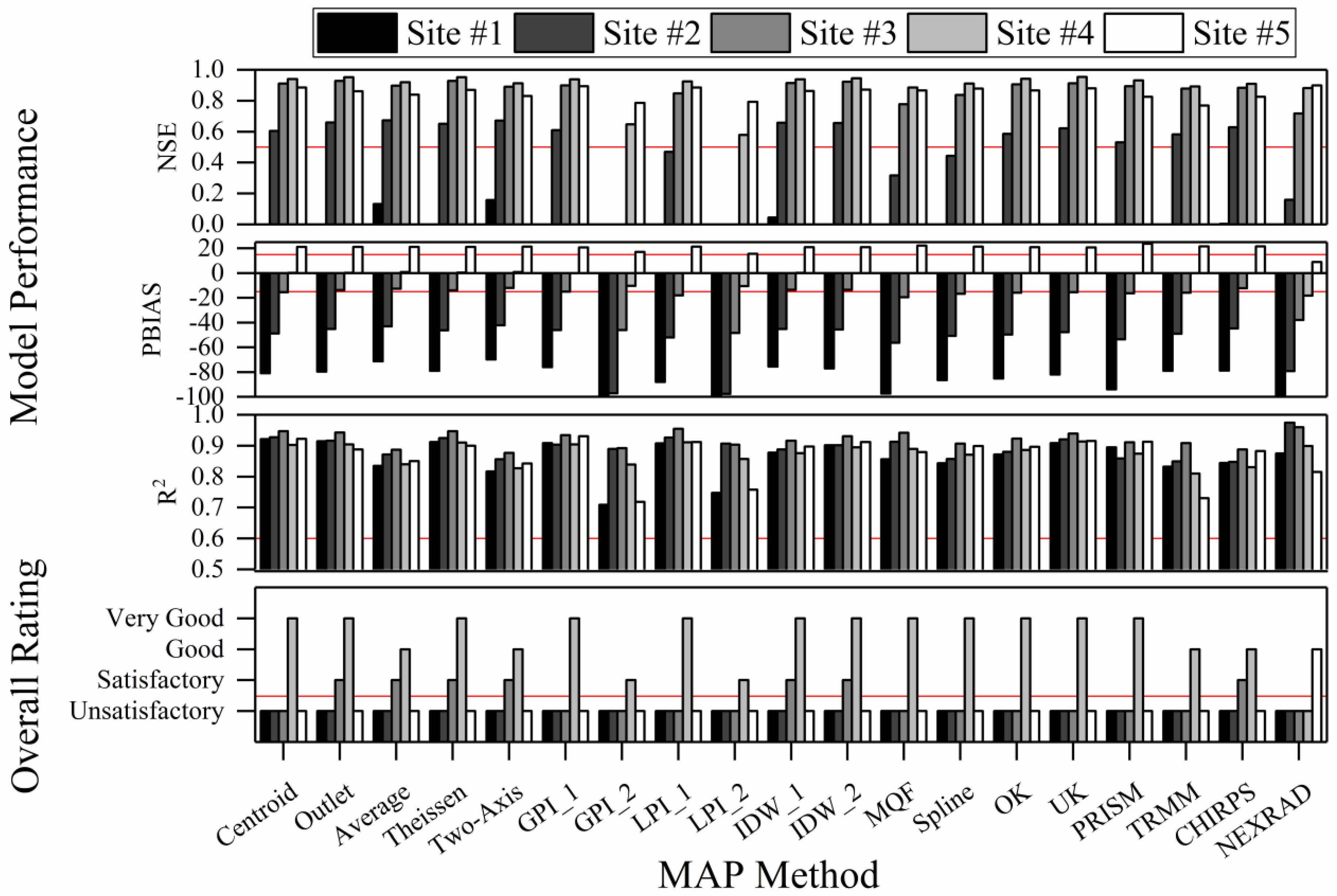
Figure 5.
Mean areal precipitation (MAP) input effects on the water balance variables (mm) after SWAT model calibration in the Hinkson Creek Watershed, Missouri, USA. SWAT models were forced with 19 different precipitation methods. Ground water is deep aquifer recharge.
Figure 5.
Mean areal precipitation (MAP) input effects on the water balance variables (mm) after SWAT model calibration in the Hinkson Creek Watershed, Missouri, USA. SWAT models were forced with 19 different precipitation methods. Ground water is deep aquifer recharge.


Table 1.
Geographic position and date range of the observed data recorded at eleven precipitation monitoring sites during water years 2009 to 2015 in Boone County, Missouri, USA. Distance to Cent. is the distance in kilometers to the centroid of the Hinkson Creek watershed.
Table 1.
Geographic position and date range of the observed data recorded at eleven precipitation monitoring sites during water years 2009 to 2015 in Boone County, Missouri, USA. Distance to Cent. is the distance in kilometers to the centroid of the Hinkson Creek watershed.
| Monitoring Site | Latitude | Longitude | Distance to Cent. (km) | Start Date | End Date |
|---|---|---|---|---|---|
| Site #1 | 39.022652° | −92.246678° | 3.803 | 1 February 2009 | 26 July 2015 |
| Site #2 | 38.981900° | −92.278671° | 1.644 | 6 February 2009 | 26 July 2015 |
| Site #3 | 38.947583° | −92.307016° | 6.053 | 8 February 2009 | 10 August 2015 |
| Site #4 | 38.927767° | −92.341505° | 9.615 | 1 March 2009 | 30 September 2015 |
| Site #5 | 38.916072° | −92.399946° | 14.34 | 13 February 2009 | 17 August 2015 |
| Sanborn Field † | 38.942301° | −92.320395° | 7.256 | 1 October 2008 | 30 September 2015 |
| Capen Park | 38.929237° | −92.321297° | 8.470 | 1 January 2011 | 30 September 2015 |
| South Farm † | 38.912626° | −92.282326° | 8.993 | 1 October 2008 | 30 September 2015 |
| Jefferson Farm † | 38.906992° | −92.269976° | 9.524 | 1 October 2008 | 30 September 2015 |
| Bradford Center | 38.897236° | −92.218070° | 11.42 | 25 April 2009 | 30 September 2015 |
| Columbia Airport | 38.818127° | −92.219672° | 19.82 | 1 October 2008 | 30 September 2015 |
† Validation sites included Sanborn Field, South Farm, and Jefferson Farm.
Table 2.
List of different mean areal precipitation (MAP) methods and associated abbreviations used in the study.
Table 2.
List of different mean areal precipitation (MAP) methods and associated abbreviations used in the study.
| Technique | MAP Method |
|---|---|
| Proximate gauge (PG) | Nearest centroid (Centoid) |
| Sub-basin outlet (Outlet) | |
| Direct-weighted average (AVE) | Arithmetic average (Average) |
| Thiessen polygons (Thiessen) | |
| Two-axis | |
| Surface-fitted (SF) | 1st order global polynomial interpolation (GPI_1) |
| 2nd order global polynomial interpolation (GPI_2) | |
| 1st order local polynomial interpolation (LPI_1) | |
| 2nd order local polynomial interpolation (LPI_2) | |
| 1st order inverse distance weighted (IDW_1) | |
| 2nd order inverse distance weighted (IDW_2) | |
| Spline tension (Spline) | |
| Multiquadric formula (MQF) | |
| Ordinary kriging (OK) | |
| Universal kriging (UK) | |
| Remotely sensed (RS) | Parameter-elevation Regressions on Independent Slopes Model (PRISM) |
| Tropical Rainfall Measuring Mission (TRMM) | |
| Climate Hazards Group InfraRed Precipitation with Station data (CHIRPS) | |
| Next Generation Radar Data (NEXRAD) |
Table 3.
Model performance ratings used to assess the SWAT model performance of stream flow.
| Performance Rating | NSE | PBIAS (%) | R2 |
|---|---|---|---|
| Very good | x > 0.8 | |x| < 5 | x > 0.85 |
| Good | 0.7 < x ≤ 0.8 | 5 ≤ |x| < 10 | 0.75 < x ≤ 0.85 |
| Satisfactory | 0.50 < x ≤ 0.7 | 10 ≤ |x| < 15 | 0.60 < x ≤ 0.75 |
| Unsatisfactory | x ≤ 0.50 | |x| ≥ 15 | x ≥ 0.60 |
Table 4.
Annual total precipitation (mm) directly measured at 11 monitoring sites during the water years from 2009 to 2015 located in Boone County, Missouri, USA.
Table 4.
Annual total precipitation (mm) directly measured at 11 monitoring sites during the water years from 2009 to 2015 located in Boone County, Missouri, USA.
| Monitoring Site | 2009 | 2010 | 2011 | 2012 | 2013 | 2014 | 2015 |
|---|---|---|---|---|---|---|---|
| Site#1 | 992 | 1646 | 794 | 660 | 1055 | 890 | 1236 |
| Site#2 | 958 | 1624 | 757 | 703 | 1077 | 946 | 1159 |
| Site#3 | 1118 | 1610 | 796 | 784 | 1034 | 917 | 1156 |
| Site#4 | 1042 | 1584 | 811 | 746 | 1054 | 915 | 1100 |
| Site#5 | 1067 | 1602 | 770 | 755 | 996 | 930 | 1091 |
| Sanborn Field † | 1088 | 1651 | 762 | 739 | 960 | 867 | 1053 |
| Capen Park | 1052 | 1463 | 795 | 738 | 976 | 891 | 1045 |
| South Farm † | 1157 | 1550 | 755 | 752 | 947 | 917 | 1093 |
| Jefferson Farm † | 1062 | 1371 | 640 | 697 | 914 | 906 | 1076 |
| Bradford | 1036 | 1412 | 689 | 733 | 916 | 883 | 1093 |
| Columbia Airport | 1018 | 1453 | 891 | 868 | 1047 | 926 | 1189 |
| All-Site Average | 1054 | 1542 | 769 | 743 | 998 | 908 | 1117 |
† Sites reserved for model validation were not included in interpolation calculations.
Table 5.
Five-site average annual mean areal precipitation (mm) estimated using 19 methods during the water years from 2009 to 2015 in Boone County, Missouri, USA.
Table 5.
Five-site average annual mean areal precipitation (mm) estimated using 19 methods during the water years from 2009 to 2015 in Boone County, Missouri, USA.
| Technique | Method | 2009 | 2010 | 2011 | 2012 | 2013 | 2014 | 2015 |
|---|---|---|---|---|---|---|---|---|
| Proximate Gauge | Centroid | 1035 | 1613 | 786 | 730 | 1043 | 920 | 1149 |
| Outlet | 988 | 1625 | 783 | 694 | 1064 | 917 | 1178 | |
| Direct- weighted Average | Average † | 1053 | 1543 | 769 | 743 | 998 | 908 | 1117 |
| Thiessen | 1025 | 1614 | 782 | 713 | 1044 | 914 | 1170 | |
| Two-axis | 1050 | 1525 | 778 | 757 | 998 | 910 | 1123 | |
| Surface-fitted | GPI_1 | 1031 | 1615 | 775 | 702 | 1042 | 918 | 1172 |
| GPI_2 | 1161 | 1767 | 802 | 738 | 1044 | 932 | 1193 | |
| LPI_1 | 1041 | 1646 | 784 | 709 | 1048 | 915 | 1186 | |
| LPI_2 | 1173 | 1791 | 812 | 747 | 1045 | 914 | 1200 | |
| IDW_1 | 1042 | 1587 | 780 | 734 | 1028 | 917 | 1148 | |
| IDW_2 | 1033 | 1604 | 780 | 723 | 1039 | 917 | 1158 | |
| Spline | 1010 | 1655 | 781 | 708 | 1044 | 924 | 1180 | |
| MQF | 1038 | 1662 | 783 | 717 | 1035 | 920 | 1184 | |
| OK | 1022 | 1612 | 781 | 719 | 1038 | 923 | 1162 | |
| UK | 1031 | 1616 | 775 | 702 | 1043 | 918 | 1172 | |
| Remotely sensed | PRISM | 1197 | 1720 | 918 | 853 | 1140 | 1073 | 1319 |
| TRMM | 1162 | 1593 | 968 | 940 | 1149 | 942 | 1203 | |
| CHIRPS | 1051 | 1595 | 911 | 828 | 1105 | 1034 | 1252 | |
| NEXRAD | 1236 | 1759 | 1027 | 892 | 1100 | 1068 | 1260 |
† Arithmetic average off all sites resulted in only one annual total precipitation value for the entire watershed.
Table 6.
Validation results showing the error associated with surface-fitted and remotely sensed annual total precipitation in the Hinkson Creek Watershed, Missouri, USA.
Table 6.
Validation results showing the error associated with surface-fitted and remotely sensed annual total precipitation in the Hinkson Creek Watershed, Missouri, USA.
| Technique | Method | RMSE | MAE | PBIAS |
|---|---|---|---|---|
| Surface-fitted | GPI_1 | 68.2 | 55.5 | −4.6 |
| GPI_2 | 69.2 | 57.0 | −5.1 | |
| LPI_1 | 63.2 | 51.8 | −4.5 | |
| LPI_2 | 68.1 | 55.8 | −5.1 | |
| IDW_1 | 66.9 | 54.2 | −4.7 | |
| IDW_2 | 67.7 | 54.7 | −5.1 | |
| MQF | 65.5 | 53.3 | −5.0 | |
| Spline | 64.6 | 53.4 | −5.0 | |
| OK | 63.5 | 52.2 | −4.6 | |
| UK | 68.2 | 55.4 | −4.6 | |
| Remotely sensed | PRISM | 148.3 | 139.2 | −13.8 |
| TRMM | 148.7 | 121.9 | −11.4 | |
| CHIRPS | 123.5 | 107.7 | −9.8 | |
| NEXRAD | 166.8 | 152.5 | −14.7 |
Table 7.
Mean areal precipitation (MAP) input effects on the uncalibrated SWAT model performance results and ratings at daily, monthly, and annual time steps after the SWAT model calibration in the Hinkson Creek Watershed, Missouri, USA. SWAT models were forced with 19 different precipitation methods. MAP methods are presented by the overall model performance rank (i.e., high to low rank).
| Overall Rank | Technique | Method | PBIAS (%) | Daily | Monthly | Annual | |||
|---|---|---|---|---|---|---|---|---|---|
| NSE | R2 | NSE | R2 | NSE | R2 | ||||
| 1 | RS | PRISM | −11.6 | 0.16 | 0.26 | 0.71 | 0.72 | 0.92 | 0.90 |
| 2 | SF | IDW_2 | 14.9 | 0.40 | 0.45 | 0.67 | 0.69 | 0.89 | 0.88 |
| 3 | SF | IDW_1 | 15.1 | 0.41 | 0.45 | 0.68 | 0.70 | 0.89 | 0.86 |
| 4 | SF | LPI_1 | 9.40 | 0.26 | 0.41 | 0.58 | 0.61 | 0.91 | 0.91 |
| 5 | PG | Outlet | 16.4 | 0.41 | 0.45 | 0.69 | 0.71 | 0.89 | 0.88 |
| 6 | SF | OK | 13.9 | 0.39 | 0.45 | 0.63 | 0.65 | 0.87 | 0.88 |
| 7 | SF | GPI_1 | 13.9 | 0.33 | 0.43 | 0.63 | 0.64 | 0.91 | 0.90 |
| 8 | SF | UK | 13.9 | 0.33 | 0.43 | 0.63 | 0.64 | 0.91 | 0.90 |
| 9 | SF | MQF | 8.9 | 0.27 | 0.42 | 0.57 | 0.60 | 0.89 | 0.88 |
| 10 | SF | Spline | 11.8 | 0.36 | 0.44 | 0.63 | 0.64 | 0.87 | 0.85 |
| 11 | AVE | Thiessen | 15.3 | 0.36 | 0.43 | 0.63 | 0.65 | 0.90 | 0.90 |
| 12 | RS | TRMM | 3.90 | 0.26 | 0.31 | 0.53 | 0.53 | 0.87 | 0.79 |
| 13 | AVE | Two-Axis | 17.0 | 0.42 | 0.44 | 0.65 | 0.69 | 0.85 | 0.82 |
| 14 | AVE | Average | 18.2 | 0.42 | 0.45 | 0.65 | 0.69 | 0.85 | 0.84 |
| 15 | PG | Centroid | 17.2 | 0.36 | 0.44 | 0.63 | 0.65 | 0.87 | 0.88 |
| 16 | SF | GPI_2 | −11.4 | −0.24 | 0.33 | 0.14 | 0.48 | 0.72 | 0.87 |
| 17 | SF | LPI_2 | −15.1 | −0.33 | 0.33 | 0.02 | 0.47 | 0.64 | 0.86 |
| 18 | RS | NEXRAD | −25.5 | 0.13 | 0.25 | 0.59 | 0.63 | 0.82 | 0.90 |
| 19 | RS | CHIRPS | 17.1 | 0.26 | 0.27 | 0.49 | 0.52 | 0.84 | 0.80 |
Table 8.
Mean areal precipitation (MAP) input effects on the calibrated SWAT model performance results and ratings at daily, monthly, and annual time steps after the SWAT model calibration in the Hinkson Creek Watershed, Missouri, USA. SWAT models were forced with 19 different precipitation methods. MAP methods are presented by the overall model performance rank (i.e., high to low rank).
| Overall Rank | Technique | Method | PBIAS (%) | Daily | Monthly | Annual | |||
|---|---|---|---|---|---|---|---|---|---|
| NSE | R2 | NSE | R2 | NSE | R2 | ||||
| 1 | SF | IDW_2 | 0.00 | 0.41 | 0.48 | 0.74 | 0.74 | 0.95 | 0.89 |
| 2 | SF | IDW_1 | 0.16 | 0.40 | 0.47 | 0.77 | 0.77 | 0.94 | 0.88 |
| 3 | SF | UK | 0.00 | 0.18 | 0.41 | 0.67 | 0.68 | 0.95 | 0.91 |
| 4 | SF | GPI_1 | 0.02 | 0.34 | 0.49 | 0.65 | 0.70 | 0.94 | 0.90 |
| 5 | RS | PRISM | 0.00 | 0.36 | 0.38 | 0.68 | 0.69 | 0.93 | 0.87 |
| 6 | PG | Centroid | 0.16 | 0.36 | 0.47 | 0.69 | 0.70 | 0.94 | 0.90 |
| 7 | PG | Outlet | 0.18 | 0.31 | 0.44 | 0.75 | 0.75 | 0.95 | 0.90 |
| 8 | SF | OK | 0.02 | 0.30 | 0.44 | 0.71 | 0.71 | 0.94 | 0.89 |
| 9 | AVE | Average | 0.77 | 0.41 | 0.48 | 0.77 | 0.77 | 0.92 | 0.84 |
| 10 | SF | Spline | 0.01 | 0.35 | 0.46 | 0.68 | 0.69 | 0.91 | 0.87 |
| 11 | SF | LPI_1 | 0.01 | 0.29 | 0.45 | 0.57 | 0.65 | 0.93 | 0.91 |
| 12 | AVE | Thiessen | 0.42 | 0.36 | 0.46 | 0.68 | 0.69 | 0.95 | 0.91 |
| 13 | AVE | Two-Axis | 0.91 | 0.37 | 0.47 | 0.76 | 0.76 | 0.91 | 0.83 |
| 14 | SF | MQF | 0.01 | 0.27 | 0.42 | 0.57 | 0.62 | 0.89 | 0.89 |
| 15 | RS | NEXRAD | −18.2 | 0.38 | 0.40 | 0.71 | 0.75 | 0.88 | 0.90 |
| 16 | RS | TRMM | −0.01 | 0.24 | 0.32 | 0.58 | 0.58 | 0.89 | 0.81 |
| 17 | RS | CHIRPS | 0.03 | 0.26 | 0.29 | 0.59 | 0.60 | 0.91 | 0.83 |
| 18 | SF | GPI_2 | −10.4 | 0.12 | 0.35 | 0.18 | 0.43 | 0.65 | 0.84 |
| 19 | SF | LPI_2 | −10.5 | −0.02 | 0.38 | 0.23 | 0.47 | 0.58 | 0.86 |
Table 9.
Mean areal precipitation (MAP) input effects on water balance variables after SWAT model calibration in the Hinkson Creek Watershed, Missouri, USA. SWAT models were forced with 19 different precipitation methods. All results are shown in depth of water (mm). The percent of total water input is shown parenthetically. Precip. is precipitation, ET is evapotranspiration, and Ground water is deep aquifer recharge.
| Technique | MAP Method | Precip. | ET | Surface Runoff (mm) (%) | Baseflow | Soil Water | Ground Water |
|---|---|---|---|---|---|---|---|
| Proximate gauge | Centroid | 1039 | 537 (52) | 412 (40) | 51 (5) | 37 (4) | 3 (0) |
| Outlet | 1036 | 536 (52) | 402 (39) | 56 (5) | 42 (4) | 4 (0) | |
| Direct-weighted average | Average | 1019 | 604 (59) | 316 (31) | 51 (5) | 48 (4) | 3 (0) |
| Thiessen | 1037 | 532 (51) | 402 (39) | 59 (6) | 45 (4) | 4 (0) | |
| Two-Axis | 1020 | 540 (53) | 386 (38) | 56 (5) | 38 (3) | 4 (0) | |
| Surface-fitting | GPI_1 | 1036 | 552 (53) | 382 (37) | 62 (6) | 40 (3) | 4 (0) |
| GPI_2 | 1091 | 597 (55) | 272 (25) | 190 (17) | 31 (2) | 9 (1) | |
| LPI_1 | 1047 | 562 (54) | 388 (37) | 59 (6) | 38 (3) | 3 (0) | |
| LPI_2 | 1097 | 598 (55) | 274 (25) | 179 (16) | 46 (3) | 8 (1) | |
| IDW_1 | 1034 | 536 (52) | 393 (38) | 64 (6) | 41 (4) | 4 (0) | |
| IDW_2 | 1036 | 536 (52) | 404 (39) | 57 (6) | 40 (3) | 3 (0) | |
| MQF | 1043 | 546 (52) | 322 (31) | 129 (12) | 46 (4) | 7 (1) | |
| Spline | 1048 | 542 (52) | 388 (37) | 73 (7) | 46 (4) | 4 (0) | |
| OK | 1037 | 530 (51) | 395 (38) | 66 (6) | 46 (4) | 4 (0) | |
| UK | 1037 | 537 (52) | 399 (38) | 58 (6) | 43 (4) | 3 (0) | |
| Remotely sensed | PRISM | 1174 | 645 (55) | 320 (27) | 151 (13) | 58 (4) | 8 (1) |
| TRMM | 1137 | 637 (56) | 380 (33) | 73 (6) | 46 (4) | 4 (0) | |
| CHIRPS | 1111 | 574 (52) | 440 (40) | 54 (5) | 44 (4) | 4 (0) | |
| NEXRAD | 1192 | 618 (52) | 275 (23) | 249 (21) | 49 (3) | 11 (1) |
© 2017 by the authors. Licensee MDPI, Basel, Switzerland. This article is an open access article distributed under the terms and conditions of the Creative Commons Attribution (CC BY) license (http://creativecommons.org/licenses/by/4.0/).
Share and Cite
MDPI and ACS Style
Zeiger, S.; Hubbart, J. An Assessment of Mean Areal Precipitation Methods on Simulated Stream Flow: A SWAT Model Performance Assessment. Water 2017, 9, 459. https://doi.org/10.3390/w9070459
AMA Style
Zeiger S, Hubbart J. An Assessment of Mean Areal Precipitation Methods on Simulated Stream Flow: A SWAT Model Performance Assessment. Water. 2017; 9(7):459. https://doi.org/10.3390/w9070459
Chicago/Turabian StyleZeiger, Sean, and Jason Hubbart. 2017. "An Assessment of Mean Areal Precipitation Methods on Simulated Stream Flow: A SWAT Model Performance Assessment" Water 9, no. 7: 459. https://doi.org/10.3390/w9070459
Note that from the first issue of 2016, this journal uses article numbers instead of page numbers. See further details here.