A Simple Model of the Variability of Soil Depths


1
Department of Earth and Environmental Sciences, Wright State University, 3640 Colonel Glenn Highway, Dayton, OH 45435, USA
2
Earth Sciences Division, E. O. Lawrence Berkeley Laboratory, 1 Cyclotron Road, Berkeley, CA 94720, USA
3
Department of Physics and Department of Earth & Environmental Sciences, Wright State University, 3640 Colonel Glenn Highway, Dayton, OH 45435, USA
4
Department of Petroleum and Geosystems Engineering, University of Texas at Austin, Austin, TX 78712, USA
*
Author to whom correspondence should be addressed.
Water 2017, 9(7), 460; https://doi.org/10.3390/w9070460
Submission received: 27 March 2017
/
Revised: 13 June 2017
/
Accepted: 19 June 2017
/
Published: 26 June 2017
(This article belongs to the Special Issue Advances in Groundwater Flow and Solute Transport: Pushing the Hidden Boundary)
Abstract
:Soil depth tends to vary from a few centimeters to several meters, depending on many natural and environmental factors. We hypothesize that the cumulative effect of these factors on soil depth, which is chiefly dependent on the process of biogeochemical weathering, is particularly affected by soil porewater (i.e., solute) transport and infiltration from the land surface. Taking into account evidence for a non-Gaussian distribution of rock weathering rates, we propose a simple mathematical model to describe the relationship between soil depth and infiltration flux. The model was tested using several areas in mostly semi-arid climate zones. The application of this model demonstrates the use of fundamental principles of physics to quantify the coupled effects of the five principal soil-forming factors of Dokuchaev.
1. Introduction
The concepts of soil formation have been extensively examined, starting from the beginning of the 19th century (Justus von Leibig: see http://www.madehow.com/knowledge/Justus_von_Liebig.html), and thereafter modified and refined by many world-renowned soil scientists, e.g., Charles Darwin [1] in England, Vasily Dokuchaev [2] in Russia, and Grove Karl Gilbert [3], George Nelson Coffey [4], and Eugene W. Hilgard [5] in the United States. The conceptual approaches to a pedogenic theory proposed by many scientists are fundamentally different, and have been revisited many times [6,7,8]. Although these theories are conceptually different, they all generally converge over the idea of Dokuchaev’s five natural soil-forming factors: biota impact, climate impact, initial material, terrain, and time, as quoted in both Glinka [9] and Jenny [10]. Dokuchaev, as quoted in Glinka [9], emphasized the necessity to determine the solution of the soil-forming factor equation, stating that:
The consideration of these theories and factors provide together a more comprehensive view of soil formation than either can do alone [11] for different types of landscapes, including those dominated by exposed bedrock, or fertile soils.In the first place we have to deal here with a great complexity of conditions affecting soil; secondly, these conditions have no absolute value, and, therefore, it is very difficult to express them by means of figures; finally, we possess very few data with regard to some factors, and none whatever with regard to others. Nevertheless, we may hope that all these difficulties will be overcome with time, and the soil science will truly become a pure science.
For later reference, soils are most commonly divided into three horizons or layers: O, A, and B, although the E, P, and C horizons are also fairly commonly discussed. In short, the O layer, present in forests, but not grasslands, is dominated by organic material, e.g., decaying plant or animal matter. The A and B layers were defined originally by Dokuchaev; the A horizon being the topsoil or humus, which is typically brown or black due to its high organic content, while the B layer is called the subsoil, and is typically more brightly colored due to the presence of clay minerals and iron oxides. However, even the full traditional classification scheme does not capture the modern understanding of soil evolution completely.
The evaluation of the lower boundaries of soil is important for many scientific and practical applications, such as agricultural and hydrological studies [12]. The depth of the soil mantling the Earth’s surface tends to vary from a few centimeters to several meters or even tens of meters [13], depending on many natural and environmental factors. For example, Hillel [14] described soil as the “top meter or so of the Earth’s surface, acting as a complex biophysical organism”. It is well recognized that an understanding and a prediction of how and where water infiltrates from the land surface and moves through the vadose zone within a landscape controls the process of biogeochemical weathering, and soil hydrology can be used to explain soil morphology and an ecosystem’s dynamical functions [12]. It has been proven that soil is being transformed globally from natural to human-affected material, the lower boundary of soil is much deeper than the solum historically confined to the O to B horizons, and most soils are a kind of paleosol, being products of many soil-forming processes that have ranged widely over the lifespans of most soils. In other words, a soil’s polygenesis is dependent on fluxes of matter and energy, which are thermodynamically transforming soil systems [15,16]. Nevertheless, when one compares predictions with data for soil depth, it is necessary at least to hypothesize the relevance of theory to a particular boundary, which we have consistently chosen to be the bottom of the soil Bw horizon, an oxidation depth.
We pose the question: are these soil fluxes dependent on infiltration from the land surface, and does the spatial variability of infiltration underlie soil depth variability?
Water flow, soil erosion (and deposition), and soil formation all affect soil depth. Soil erosion is chiefly accomplished through advective processes such as overland flow and rainsplash [17], though soil creep and a number of other processes contribute as well. Biogeochemical weathering, a basis of soil formation, requires water to carry reaction reagents to the weathering front, and reaction products away [18], and thus relates to deep infiltration. Erosion rates vary over about 4 orders of magnitude, from a fraction of a meter per million years in the interior of Australia, to a maximum of over 1000 m per million years in the Himalayas [19]. Precipitation rates vary from 2 mm/year in the Atacama Desert to 10 m/year in the New Zealand Alps (and in many other regions). The soil production rate is linearly proportional to precipitation [18,20], and has been reported as an exponentially diminishing function of soil depth [21], though the “humped” function was reported in several recent studies; see Heimsath et al. [22]. Soil erosion and soil production must be correlated, which is a stipulation guaranteed by the conditions of an apparent steady-state landscape evolution, but is also possible if the fundamental physical processes controlling the soil formation processes are related, even when steady-state conditions do not apply.
Historically, soil formation s has been represented in terms of a single formula, in which the principle factors of formation s = f (cl, o, r, p, t), are represented independently from each other, e.g., cl, for climate, o for organisms, r for topography (relief), p for parent material, and t for time [9,10]. A guiding convention has been that soil is predominantly formed due to biogeochemical weathering, as a combination of physical, chemical, thermal, and biological processes together causing the disintegration of rocks, an evolutionary process that does not stop with the initial formation of soil. These processes, themselves, are limited by the atmosphere–rhizosphere, subsurface interaction, and in particular, infiltration from the land surface and solute transport in the unsaturated (vadose) zone. For example, organisms and precipitation supply the CO2 necessary to drive silicate-weathering processes [23]. Soil processes are also affected by erosion, deposition, (e.g., aeolian) plant root uptake, microbial processes, infiltration, and evapotranspiration.
In the following, we present the general model. Then, we test it: first to see whether the values of the typical input variables generate values in accord with typical soil depths around the globe, then to see whether it reproduces variability in soil depth in accord with that observed over variable climatic input and what is known about parent material particle size variability with respect to topography (slope). Finally, we consider the implications of our model treatment and its wide range of applicability for landscape evolution concepts and discussions of agricultural sustainability.
2. General Model
The model for soil formation derives from percolation theory for solute transport in porous media. Percolation theory can be applied to enumerate the dominant flow paths when the medium is highly disordered. Chemical weathering in situ is shown to be transport-limited [24,25], but the lower boundary of chemical weathering is the bottom of the B horizon. The soil depth, neglecting erosion, is taken to be the distance of solute transport [18]. Percolation concepts that relate solute transport time and distance thus relate soil age and depth through the process of transport-limited chemical weathering [24].
It has been shown [18] that, when erosion (and deposition) can be neglected,
Equation (1) describes the evolution of soil depth x as a function of time t. This expression has been derived based on the results of field and laboratory investigations of solute transport [25,26] associated with the chemical weathering of soil. It has also been assumed that this equation can be used to describe the bottom depth of the Bw horizon. Here, Db = 1.87 is the fractal dimensionality of the percolation backbone for vertical flow, with 1.87 valid for full saturation and three-dimensional connectivity. In percolation theory, the backbone is obtained from the dominant, optimally connected flow paths by trimming off portions that connect only at one spot, called dead-ends. The mass fractal dimension of the backbone provides the scaling exponent relating time and distance. Predominantly downward flow occurs also under wetting conditions, but in this case the correct exponent is only slightly different, with Db = 1.861, an insignificant difference from 1.87. In this expression, x0 is a characteristic particle size of the soil parent material, and (x0/t0) ≡ I/φ, with
where I is the net infiltration rate; φ is the soil porosity (used to change the Darcy velocity to the pore-scale velocity); P is precipitation; and AET is the average evapotranspiration. The soil production function is then given by
I = P − AET + run-on − run-off,
dx/dt = (1/Db) (x0/t0) (x0/x)Db − 1.
Erosion is assumed to be taken into account by subtracting a constant, E, from the right-hand side of the differential equation. When soil erosion and soil production processes are equal in magnitude, dx/dt = 0, and the soil depth, x, is given by the equation
The power 1.15 of Equation (2) is 1/(Db − 1).
Equations (1) and (2) implicitly represent a combination of the effects of climate, topography, and evapotranspiration. Equation (2) does not contain a time variable, since this equation represents the solution of Equation (1), consistent with an asymptotical convergence of the soil formation depth to a steady state value.
3. Predicting a Typical Soil Depth
If a typical soil depth is a depth you would expect to measure, this equates the term, in a narrow sense at least, to a mean soil depth. However, the actual values of soil depths vary from zero to tens of meters. What is a typical soil depth? Batjes [26], who considered the 4353 soils in the World Inventory of Soil Emission (WISE), used it to build up UNESCO’s (United Nations Educational, Scientific, and Cultural Organization) database of 106 soil types presented on its soil map, assuming a characteristic soil depth of 1 m. Montgomery [27] gives a mean soil depth of 1.09 m, with a mean soil depth of 2.74 m for native vegetation, and 2.01 m for soil production areas. Hillel suggested that 1 m is a typical soil depth. What value would be suggested by Equation (2)?
Take x0 = 30 μm, the size of a typical silt particle. Silt is the middle particle size (geometric mean) class in all soil classification schemes, and 30 μm is the middle (arithmetic mean) of the silt range. The same value, 30 μm, is also the geometric mean of the individual arithmetic means of the three principal soil particle classes, clay, silt, and sand. This particular length scale relates most closely to parent material, whether the soil is weathering from a bedrock with a specific mineral size, or whether it is forming on, e.g., an alluvial deposition. To calculate a mean infiltration rate, we must consider not only the precipitation, but also the water lost to evaporation and transpiration as well as what runs off. These variables relate to climate, the hydraulic conductivity of the substrate, and to the role of plants in the water cycle. Schlesinger and Jasechko [28] estimate that, globally, transpiration constitutes 61% of AET, and returns approximately 39% of P to the atmosphere. Thus, AET represents a mean fraction (0.39/0.61) = 64% of P. Lvovich’s [27] estimation that AET = 65% of P is almost identical, and he also gives a global mean precipitation of 834 mm. Lvovich [29] estimates that a global mean of 24% of P travels to streams by overland flow, leaving only 11% of P for deep infiltration. The mean terrestrial P is reported as between 850 mm and 1100 mm [30], with a mean of 975 mm. Sixty-four percent of 975 mm is 624 mm, leaving 351 mm for P − AET. However, 11% of 975 mm is only 102 mm. On any local site, however, the difference between the run-on and the run-off can be either positive or negative. Thus, these estimates suggest that the amount of water reaching the base of the soil should be a column of water somewhere between 102 mm and 351 mm. Alternatively, we can consider the mean global AET over cold, temperate, and tropical, forested and non-forested, regions. Using the six different values given by Peel et al. [31] for these biomes generates an AET value of 654 mm, which is fairly close to the value inferred from Schlesinger and Jasechko [28], and implying P − AET = 321 mm. The actual infiltration rate is obtained from I through division by the porosity. We assume a typical porosity of 0.4, leading to values of I/φ between 255 mm/year and 878 mm/year (using a combination of Schlesinger and Willmott’s numbers), or between 225 mm/year and 735 mm/year (using the numbers of Lvovich). These values average to 566 mm/year, or 480 mm/year, depending on the particular estimates applied, and are reasonable. A typical erosion rate of about E = 30 m/Myear ≈ [(1 m/Myear) (1000 m/Myear)]0.5, is obtained from the geometric mean of the range of erosion rates discussed in Bierman and Nichols [19]. Using x0 = 0.00003 m, I/φ = 806 mm/year, and E = 30 m/Myear, and the first range of I values given, the result for x is 0.48 m < x < 1.81 m, while for the second range of I values given, 0.42 m < x < 1.53 m. Both the arithmetic and geometric means of both ranges cluster around 1 m.
4. What Can We Say about the Variability of Soil Depths?
Let us consider first the ratio I/E, which, raised to the power 1.15, has the potential to produce the greatest variation (range) in soil depths. In fact, this ratio should be quite insensitive to P, since both I and E tend to increase with increasing precipitation. For example, Dunne et al. [32] found a linear relationship between I and P, in general accord with the previously cited tendency for AET to be roughly half of P. Reiners et al. [33] reported a linear relationship between P and erosion, E. Their study utilized a rainfall gradient at similar temperatures across the Cascade Mountains in Washington State, United States. Along this transect one should thus expect roughly constant soil depths, and the ratio I/E should, in the absence of steep topography, remain relatively invariant. What about trends with temperature? Data from Sanford and Selnick [34] revealed a tendency for the fraction of precipitation lost to AET to increase with increasing temperature, particularly in conjunction with aridity. Thus, the conclusions of Heimsath et al. [35] regarding the results of their Australian measurements, “[t]he suite of results from different field sites indicates that erosion rates generally increase with increasing precipitation and decreasing temperature,” indicate that the processes of soil formation may be dependent on evapotranspiration. Consequently, the water potentially available for either infiltration or overland flow, (P − AET), serves as a predictor of E and soil formation, rather than simply P. We, therefore, hypothesize that both the numerator and denominator in Equation (1) would contain a proportionality to the quantity (P − AET), meaning that weather conditions (within a specific climatic zone) would have far less influence on soil depth than commonly assumed. However, I and E can be expected to have a complementary dependence on the partitioning of water to overland flow, which brings in the effect of topography. The relationship between the potential evaporation, evapotranspiration, precipitation, and runoff was considered in great detail by Budyko [36], and many soil scientists and hydrologists followed Budyko’s approach, e.g., Gentine et al. [37].
Concerning topography, regions with steeper topography will tend to have higher overland flow, and thus higher erosion rates, resulting in lower infiltration and soil formation rates. As an example, Burbank et al. [38] found that erosion rates and precipitation in the Himalayan mountains were not correlated (in contrast to Reiners et al. [33]), and attributed their anomalous result to the strong tendency for the precipitation to decline where the slope was increasing. Notably, however, the declining precipitation with increasing slope should lead to a diminution in soil production compared with erosion, and a higher probability of bedrock exposure, as is indeed the case in this region. Divergent topography, with concomitant divergence in surface water flux and therefore soil transport, will produce thinner soils than convergent topography, as noted in Heimsath et al. [39], a tendency intensified by steeper topography generally. Our reasoning, though it may be accentuated in reality by lateral soil transport [39], does not depend on such transport, and is merely a consequence of the greater infiltration values in topography that is convergent and not so steep that soil covering is missing entirely.
How does soil depth depend on the particle size of original sediments? This question is more nuanced than the previous question. Soil depths should nominally be proportional to particle sizes. However, erodibility has a strong dependence on particle size, first increasing with increasing size from clay to silt, and then decreasing with increasing size at larger sizes. The seeming anomaly at small particle sizes is due to the cohesive forces between clay grains, which are typically charged. Thus, as long as I is principally precipitation-limited, a decrease in particle size below silt size tends to reduce soil erosion, on account of the increasing cohesive forces between the grains. Therefore, x0, for finer soils at least, should be positively correlated with the erosion rate, E, and the two stated influences will tend to cancel. However, at larger particle sizes, increasing particle sizes should tend to decrease E, accentuating the tendency for soils to be deeper; although, if the argument is turned around, a greater importance of erosion will tend to remove finer components, leading to a coarser soil. Sandy soils should thus have the deepest weathering horizons, although for larger particle sizes, the term soil is not characteristically employed. If I is principally hydraulic conductivity-limited, however, then greater precipitation rates, P, will not tend to increase I, but will tend to increase water run-off and erosion, E, leading to much thinner soil depth, regardless of particle size. Thus, unfractured crystalline rock with very low hydraulic conductivity values will tend to be exposed, unless it is buried through, e.g., fluvial deposition. Similar conclusions hold for increased slope angles, which will increase E and, more likely, decrease I, both of which should lead to thinner soils.
Finally, it is worth noting that, especially for very low soil formation rates and erosion rates in, e.g., continental interiors such as Australia [40], soil formation rates do tend to be larger than soil erosion rates, consistent with the predicted power-law decay of the soil production function (rather than the oft-assumed exponential form of Heimsath et al. [41]). The slow decay toward a steady-state soil production value leads to an increased tendency of soils in arid regions not to attain steady-state conditions [40], and for their depths to be smaller than that predicted from steady-state landscape evolution assumptions.
5. Comparison With Data: Mainly Climate
Below, we use data of White et al. [42], He et al. [43], Egli et al. [44] the Heimsath group [35,39,45,46,47], to confirm the relative consistency of soil depths across climatic gradients, but not across a variation in topography. The San Gabriel Mountain data of Southern California [45] demonstrate the variation of soil depths along a gradient in topographic relief, and thus erosion rates, but not of climate. We have found particle size data for only five of the data sets below, and even in some of these cases we had to generate a median particle size from graphic representations of what are considered to be typical distributions of particle diameters for a given texture [48].
In southeastern Australia, where many of the Heimsath group’s field sites are located, precipitation tends to increase inland up to the escarpment, and then decrease with increasing altitude. The decrease in P with increasing altitude is mirrored by a diminution in AET from between 600 mm/year and 700 mm/year, to between 500 mm/year and 600 mm/year [49]. The Frog’s Hollow and Brown Mountain sites at about 1000 m elevation have more limited vegetation cover and cooler temperatures compared with Nunnock River and Snug, both factors that tend to reduce evapotranspiration.
In the San Gabriel Mountains, “the landscape varies from gentle, soil mantled and creep dominated in the west to steep, rocky and landslide dominated in the east”, accompanied by an increase in erosion rates from about 35 m/Myear to over 200 m/Myear, with the boundary to landslide dominated at about 200 m/Myear. The actual soil depth extremes were taken from Figure 3 of Heimsath et al. [45], and restricted to non-landslide-dominated slopes. On landslide-dominated slopes, the soil depth was “patchy”, a scenario not addressed here. Thus, the variation in soil depth from west to east along the San Gabriel Mountains is a result of a variation in the erosion rate due to changes in mountain slope, rather than a variation in, e.g., climatic variables. Net infiltration rates are calculated as I = P − AET − Run-off, given the fact that run-off tends to be higher than run-on, and can play a role in water loss on site (according to Lvovich [29], 24% of precipitation flows into the ocean through surface run-off globally, while only 11% goes into deep infiltration). A summary of predicted and observed soil depths over two orders of magnitude of erosion rates is given in Table 1. Our predicted mean soil depth across 12 sites on four continents is 1.14 m, while the observed mean soil depth across those sites is 0.81 m.
In Figure 1, we compare predicted and observed soil depths, forcing the linear fit to go through the origin (for the San Gabriel Mountains, mean values are used here). We have an overall 43% overestimation for the mean soil depths across 12 sites, with less than 15% discrepancy at 3 sites, and 5 out of 12 underestimations (~22% on average) along with 7 overestimations (~90% on average). A large fraction of the overestimation comes from Merced River (84%), which has a slow average erosion rate and might not have reached a steady-state condition, and from east of the San Gabriel Mountains (200% to 500%) with a very shallow observed soil depth of 3 cm, which contributes a large discrepancy to the percentage, if not the actual discrepancy. There are a number of other potential reasons for overestimation. Our choice of an arithmetic mean for the observed soil depths tends to minimize the influence of shallower soil depths in the reporting of regional values for soil depth, but younger, shallower soils still tend to reduce a mean depth compared with a predicted steady-state value. Other sources of errors could come from reducing an entire particle size distribution to a median particle size, the accuracy of P, AET, and Run-off rates, and the porosity of the soils, particularly since we do not have a means to address local variability for most sites. Note that removing Merced River (maximum predicted value) will result in reducing R2 from 0.934 to 0.679, while decreasing the numerical pre-factor from 1.66 to 1.05, making the relationship nearly one-to-one.
6. Comparison with Data: Slope Angle
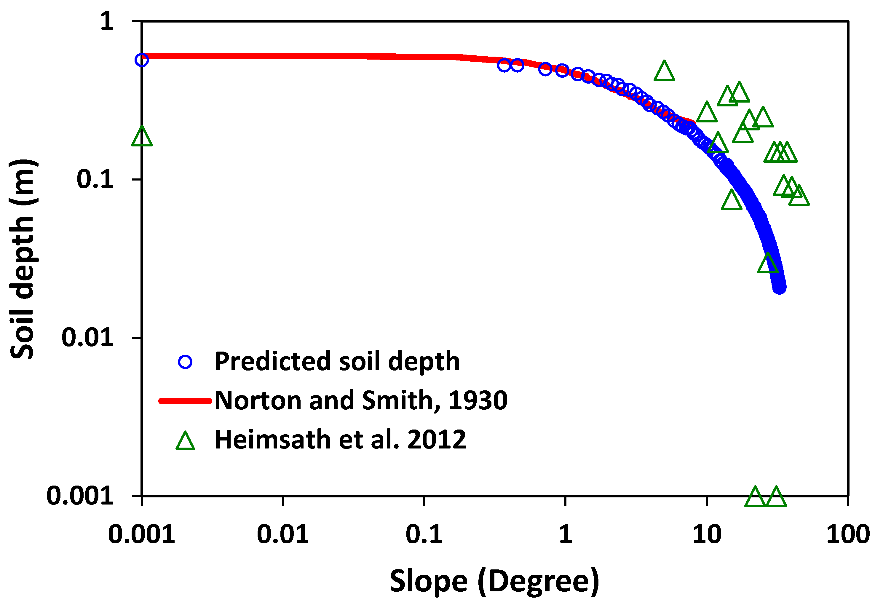
Let us consider specifically the slope angle dependence of soil depth as exhibited by the data from the San Gabriel Mountains [45] and a result from Norton and Smith from 1930 as reported in Jenny [10]. We apply Equation (2) with the known value of P − AET − run-off from Table 1, and a 30 μm median particle diameter. In order to address the slope dependence of soil depth, Equation (2) requires a slope-dependent erosion rate. Although it is not within our capability to predict such a function, Mongomery and Brandon [60] reported in their Figure 1 an empirical function for the slope angle dependence of erosion rates in the Olympic Mountains in Washington. Incorporating this empirical input makes it possible to use Equation (2) to predict the slope angle dependence of soil depth. The comparison is shown in Figure 2. In order to make this equation predictive, the input of the erosion rate function (Montgomery and Brandon [60]) is critical. This function tends to produce a rapid reduction in soil depths to nearly zero as slopes of about 30 degrees are exceeded (since zero values cannot be plotted on a logarithmic graph, such values were converted to 0.001 for both axes). In spite of the considerable scatter in field values, it appears that our prediction captures the essential trends accurately. Note that the use of either 20 μm or 30 μm for the fundamental particle size will result in an overestimation of the soil depth at zero slope, but an underestimation at larger slopes, since the latter values are deeper than the zero slope depths, a result attributed by the authors [45] to the effects of soil deposition.
7. Implications for Geomorphological Studies of Natural and Agricultural Landscapes
The existing landscape evolution models require a large number of inputs, such as soil production and soil transport as functions of depth, parent material, topography, climate, and organisms, while delivering several quantities of interest. The outputs include: (1) regional denudation rates, which are important for understanding (neo) tectonics; (2) spatial variability of soil erosion; (3) spatial variability of soil depth; and (4) spatial variability of landforms. When adapted to landscapes with human interference, such as agriculture, the second and third of these products may take on additional significance regarding sustainability. The first and fourth results typically involve larger time scales than the human time scales resolved by agricultural practices. Many processes are relevant to the evolution of landscapes, and these can have different impacts at different time scales and in different locations. We point out that the choice of soil production model has an impact on the results of such landscape evolution models, and that our soil production function may help to resolve some difficult problems in landscape evolution modeling.
When an exponential model for soil production is assumed, which delivers a maximum soil production rate modulated by an exponential decay, one finds for a steady-state soil thickness the negative of the logarithm of the ratio of the erosion rate to the maximum soil production rate, −ln (E/Rm) [61]. For a wide range of typical values for E and maximum soil production rate, Rm (as reported by Heimsath and co-workers), it turns out that this formula yields soil depths ca. 1 m. But the physical reason for a relatively consistent soil depth that lies in the correlation between E and R through the factor P − AET is missing in Roering [61] (both run-off and net infiltration, I, increase with P − AET). In Roering’s treatment, the relative consistency in the output arises from the logarithmic phenomenology, which is very slowly varying in comparison with our power law. Consider, however, what happens if I, which is the upper limit of soil production rates in our treatment, is substituted for Rm in the Roering soil thickness relationship. Since maximum soil production rates [62] are ca. 3000 m/Myear, but infiltration rates can be approximately three orders of magnitude larger, even with Roering’s logarithmic dependence, substituting I for Rm would increase the predicted soil depth considerably. Nevertheless, replacement of Rm by I in Roering’s result generates the same argument in the logarithm as appears in our power law. This is a significant correspondence. Our result expressed in Equation (2) generates, in principle, a much more sensitive function of parameters such as infiltration and erosion rates to the soil depth. However, the tendency of each to increase with increasing P − AET makes this ratio rather insensitive to changes in climate. However, see what happens if the erosion rate changes by over an order of magnitude due to topography, such as in the San Gabriel Mountains. Our result predicts a better than order of magnitude change in soil depth, as observed, as well as the approximate functional form of the soil depth as a function of slope angle (Figure 2), whereas that of Roering predicts a variation less than a factor 2 (compare the actual soil depth distinction between the western and eastern provinces of a factor approximately 20).
Although the most important topic may thus relate to absolute values of soil production and erosion, issues in the local variability of soil production and erosion relate to the shapes of the topography as well, and here understanding is also lacking. More generally, the use of common landscape models [63,64,65] does not allow for the prediction of the wide range of observed shapes of landscapes. From Roering [61], “linear transport models [use of the diffusion equation for soil downslope transport] produce constant curvature, not planar slopes, necessitating integration of various downslope transport mechanisms. Put simply, the [introduced] flux-slope nonlinearity enables nearly steep and planar (low convexity) sideslopes to erode at rates commensurate with highly convex hilltops.” As Roering points out, such problems have been addressed by incorporating soil depth-dependent transport as well as soil production into landscape evolution models [66,67], which allows an increase in soil transport rates downslope even in the case of planar slopes. However, with our result of a soil formation function which is highly dependent on infiltration, the low infiltration rate on hilltops and slopes (as compared to hollows) will tend to produce a smaller soil production rate, which could, without this strong dependence on infiltration, otherwise be interpreted as resulting from a larger erosion rate. Perhaps a portion of the difficulties encountered by landscape evolution models is that they do not incorporate sufficient local variability in soil production rates due to the convergence/divergence of surface flow.
Our results also have implications for agricultural systems. In particular, we can predict what a new steady state soil depth will be if the soil erosion rate is increased by an order of magnitude or more, as results from traditional agricultural practices. While it is possible to write an accurate result for the soil production in terms of the instantaneous depth and the erosion rate, which allows a more rigorous prediction of the time frame over which the soil adapts to the new erosion conditions, several factors suggest that it may be better to calculate this time scale simply by taking the quotient of a typical original soil depth (say 1 m) and dividing by the erosion rate. One complicating factor is that the soil production function may change when the soil is very shallow, at least if the bedrock does not have a hydraulic conductivity comparable to that of the soil. In such a case, the relevant infiltration rate may be much smaller in a very shallow soil, and the soil production function comparably reduced. Such a situation could lead to a “humped” soil production function [22], an instability resulting in total soil loss, and, essentially, a two state system, where it may be difficult for natural systems to evolve between the two, i.e., once the soil is lost, it does not return. Results for our predicted steady-state soil depths are given in Table 2 below. In the case of calculations for the time required to strip a landscape of soil, we used an arbitrary starting depth of 1 m, in approximate accord with our general predictions, Roering’s [61] equation, and, as it turns out, with steady-state depths calculated from Equation (2) in accord with the input erosion rates given by Montgomery [27].
Using a mean erosion (or soil production) rate, one finds a mean soil depth of 0.51 m, while using a median erosion rate, the result is 1.95 m, consistent with our understanding that 1 m is a typical soil depth. An important result is that, for traditional agriculture, using a typical soil depth of 1 m generates a time until virtually complete soil loss of between 250 and 650 years, a result that is consistent with Montgomery’s [68] assertion that limits on agriculture placed by soil loss were critical in setting the period of domination of a number of classical civilizations at about 500 years.
Consider some of the individual values of soil depths in Table 2. With native vegetation, the range of depths extends from 54 cm to 2.74 m. The soil production values suggest a range of soil depths from 85 cm to 2.01 m. However, the geologic erosion rates indicate steady-state soil depths from 14 cm to 1.09 m. (Note that soil degradation, i.e., soil depletion, is taking place due to a combination of factors, such as deforestation (30%), agricultural activities (28%), overgrazing (35%), overexploitation (7%), and industrialization (1%) [69]. Among factors of physical degradation are water erosion (55%), wind erosion (29%), chemical degradation (12%), and compaction/crusting (4%) [69]. Some of the more interesting results, however, may be the implied steady-state soil depths for normal agriculture, which lie between 4 mm and 11 mm, whereas the corresponding depths for conservation agriculture range from 21 cm to 33 cm. Thus, it is clear that, while normal agriculture is not sustainable, conservation agriculture is also quite marginal, as most crops need more than 33 cm of soil to thrive.
8. Summary
Based on the concept that the soil forming processes combined are dependent on the infiltration rate, we developed a simple model for the prediction of the soil depth. The model is verified by comparison of predicted and actual soil depths for a range of climates with emphasis on semi-arid zones, as well as along a slope gradient. Discrepancies between the data and model calculations remain, but they are comparatively small, taking into account the variety of soil forming factors: topography, climate, organisms, and parent material. When expressed as a function of time, it is shown to describe the temporal development of soil production. However, according to Dokuchaev and later soil scientists, it is equally important to be able to express a range of other soil forming factors, such as carbon and nitrogen content and other chemicals.
In our discussion and comparison with data, some details are still missing, such as (in most cases) site-specific porosity, or run-off values. The relevant porosity may be the effective value, which excludes pores that do not connect, or connect to flow paths at only one point, and likely excludes also internal water adsorption into clay minerals. We also have not addressed issues of climate change, which could require significant alterations of parameter values over time. It is to be hoped that a more detailed investigation of such parameter values and their potential temporal variation will improve the accuracy of our predictions. Additionally, we have not addressed specific flow paths, which may depend on a wide variety of factors, such as the slope angle, or whether the soil is graded or layered. All of these factors may introduce as yet unaccounted for variability. In spite of these omissions, the theoretical approach appears to account properly for soil formation factors over a wide range of climates and slope angles.
Author Contributions
Yu (writing, soil data location and digitization, climate and run-off data search, analysis), Hunt (conception), Faybishenko (writing, relationships to fundamental soil formation models and history of soil science), Ghanbarian (writing and analysis).
Conflicts of Interest
The authors declare no conflict of interest.
References
- Darwin, C. The Formation of Vegetable Mould through the Action of Worms, with Observations on Their Habits; John Murray: London, UK, 1881. [Google Scholar]
- Dokuchaev, V.V. Russian Chernozem. In Selected Works; Monson, S., Ed.; Israel Program for Scientific Translations Ltd.: Moscow, Russia, 1948; Volume 1, pp. 14–419. [Google Scholar]
- Gilbert, G.K. The convexity of hilltops. J. Geol. 1909, 17, 344–350. [Google Scholar] [CrossRef]
- Coffey, G.N. A study of the Soils of the United States, Bulletin 85; USDA Bureau of Soils: Washington, DC, USA, 1912; p. 114.
- Hilgard, E.W. Soils; The Macmillan Company: New York, NY, USA, 1914. [Google Scholar]
- Cline, M.G. Historical highlights in soil genesis and classification. Soil Sci. Soc. Am. J. 1977, 41, 250–254. [Google Scholar] [CrossRef]
- Richter, D.D.; Markewitz, D. Understanding Soil Change: Soil Sustainability Over Millennia, Centuries and Decades; Cambridge University Press: Cambridge, UK, 2001. [Google Scholar]
- Richter, D.D.; Yaalon, D.H. “The Changing Model of Soil” Revisited. Soil Sci. Soc. Am. J. 2011, 76, 766–778. [Google Scholar] [CrossRef]
- Glinka, K.D. Dokuchaiev’s Ideas in the Development of Pedology and Cognate Sciences, 1st ed.; Series: Akademiia Nauk SSR. Russian pedological investigations; The Academy: Leningrad, USSR, 1927. [Google Scholar]
- Jenny, H. Factors of Soil Formation: A System of Quantitative Pedology; Dover: New York, NY, USA, 1941. [Google Scholar]
- Johnson, D.L.; Schaetzl, R.J. Differing views of soil and pedogenesis by two masters: Darwin and Dokuchaev. Geoderma 2014, 237, 176–189. [Google Scholar] [CrossRef]
- Schoeneberger, P.J.; Wysocki, D.A. Hydrology of soils and deep regolith: A nexus between soil geography, ecosystems and land management. Geoderma 2005, 126, 117–128. [Google Scholar] [CrossRef]
- Glinka, K.D. Pochvovedenie, Moscow, 1931 (Translated Treatise on Soil Science by Israel Program for Scientific Translations, Jerusalem); National Science Foundation: Washington, DC, USA, 1931.
- Hillel, D. Soil: Crucible of life. J. Nat. Resour. Life Sci. Educ. 2005, 34, 60–61. [Google Scholar]
- Chizhikov, P.N. The lower boundary of soil. Sov. Soil Sci. 1968, 11, 1489–1493. [Google Scholar]
- Richter, D.D.; Bacon, A.R.; Brecheisen, Z.; Mobley, M.L. Soil in the Anthropocene. Earth Environ. Sci. 2015, 25. [Google Scholar] [CrossRef]
- Anderson, R.S.; Anderson, S.P. Geomorphology: The Mechanics and Chemistry of Landscapes; Cambridge Press: New York, NY, USA, 2010. [Google Scholar]
- Hunt, A.G.; Ghanbarian, B. Percolation theory for solute transport in porous media: Geochemistry, geomorphology, and carbon cycling. Water Resour. Res. 2016, 52, 7444–7459. [Google Scholar] [CrossRef]
- Bierman, P.R.; Nichols, K.K. Rock to sediment—slope to sea with 10Be--rates of landscape change. Annu. Rev. Earth Planet. Sci. 2004, 32, 215–255. [Google Scholar] [CrossRef]
- Amundson, R.; Heimsath, A.; Owen, L.; Yoo, K.; Dietrich, W.E. Hillslope soils and vegetation. Geomorphology 2015, 234, 122–132. [Google Scholar] [CrossRef]
- Carson, M.A.; Kirkby, M.J. Hillslope Form and Process; Cambridge University Press: Cambridge, UK, 1972; p. 475. [Google Scholar]
- Heimsath, A.M.; Fink, D.; Hancock, G.R. The ‘humped’ soil production function: eroding Arnhem Land, Australia. Earth Surf. Process. Landf. 2009, 34, 1674–1684. [Google Scholar] [CrossRef]
- Hilley, G.E.; Porder, S. A framework for predicting global silicate weathering and CO2 drawdown rates over geologic time-scales. Proc. Natl. Acad. Sci. USA 2008, 105, 16855–16859. [Google Scholar] [CrossRef] [PubMed]
- Hunt, A.G.; Ghanbarian-Alavijeh, B.; Skinner, T.E.; Ewing, R.P. Scaling of geochemical reaction rates via advective solute transport. Chaos 2015. [Google Scholar] [CrossRef] [PubMed]
- Yu, F.; Hunt, A.G. Damköhler number input to transport-limited chemical weathering and soil production calculations. ACS Earth Space Chem. 2017, 1, 30–38. [Google Scholar] [CrossRef]
- Batjes, N.H. Total carbon and nitrogen in the soils of the world. Eur. J. Soil Sci. 1996, 47, 151–163. [Google Scholar] [CrossRef]
- Montgomery, D. Soil erosion and agricultural sustainability. Proc. Natl. Acad. Sci. USA 2007, 104, 13268–13272. [Google Scholar] [CrossRef] [PubMed]
- Schlesinger, W.H.; Jasechko, S. Transpiration in the global water cycle. Agric. For. Meteorol. 2014, 189, 115–117. [Google Scholar] [CrossRef]
- Lvovitch, M.I. The global water balance: U.S. National Committee for the International Hydrological Decade. Natl. Acad. Sci. Bull. 1973, 28–42. [Google Scholar] [CrossRef]
- Willmott, C.J.; Robeson, S.M.; Feddema, J.J. Estimating continental and terrestrial precipitation averages from rain-gauge networks. Int. J. Climatol. 1994, 14, 403–414. [Google Scholar] [CrossRef]
- Peel, M.C.; McMahon, T.A.; Finlayson, B.L. Vegetation impact on mean annual evapotranspiration at a global catchment scale. Water Resour. Res. 2010. [Google Scholar] [CrossRef]
- Dunne, T.; Zhang, W.; Aubrey, B.F. Effects of rainfall, vegetation, and microtopography on infiltration and run-off. Water Resour. Res. 1991, 27, 2271–2285. [Google Scholar] [CrossRef]
- Reiners, P.W.; Ehlers, T.A.; Mitchell, S.G.; Montgomery, D.R. Coupled spatial variations in precipitation and long-term erosion rates across the Washington Cascades. Nature 2003, 426, 645–647. [Google Scholar] [CrossRef] [PubMed]
- Sanford, W.E.; Selnick, D.L. Estimation of evapotranspiration across the conterminous United States using a regression with climate and land-cover data. J. Am. Water Res. Assoc. 2013, 49, 217–230. [Google Scholar] [CrossRef]
- Heimsath, A.M.; Chappell, J.; Fifield, K. Eroding Australia: Rates and Processes from Bega Valley to Arnhem Land; Bishop, P., Pillans, B., Eds.; Australian Landscapes, Geological Society: London, UK, 2010; Volume 346, pp. 225–241. [Google Scholar] [CrossRef]
- Budyko, M.I. Climate and Life; Academic Press: Orlando, FL, USA, 1974. [Google Scholar]
- Gentine, P.; D’Odorico, P.; Lintner, B.R.; Sivandran, G.; Salvucci, G. Interdependence of climate, soil, and vegetation as constrained by the Budyko curve. Geophys. Res. Lett. 2012, 39. [Google Scholar] [CrossRef]
- Burbank, D.W.; Blythe, A.E.; Putkonen, J.; Pratt-Sitaula, B.; Gabet, E.; Oskin, M.; Barros, A.; Ojha, T.P. Decoupling of erosion and precipitation in the Himalayas. Nature 2003, 426, 652–655. [Google Scholar] [CrossRef] [PubMed]
- Heimsath, A.M.; Dietrich, W.E.; Nishiizumi, K.; Finkel, R.C. Cosmogenic nuclides, topography, and the spatial variation of soil depth. Geomorphology 1999, 27, 151–172. [Google Scholar] [CrossRef]
- Yu, F.; Hunt, A.G. An examination of the steady-state assumption in soil development models with application to landscape evolution. Earth Surf. Process. Landf. 2017. under review. [Google Scholar]
- Heimsath, A.M.; Dietrich, W.E.; Nishiizumi, K.; Finkel, R.C. The soil production function and landscape equilibrium. Nature 1997, 388, 358–361. [Google Scholar] [CrossRef]
- White, A.G.; Blum, A.E.; Schulz, M.S.; Bullen, T.D.; Harden, J.W.; Peterson, M.L. Chemical weathering rates of a soil chronosequence on granitic alluvium: I. Quantification of mineralogical and surface area changes and calculation of primary silicate reaction rates. Geochimi. Cosmochim. Acta 1996, 60, 2533–2550. [Google Scholar] [CrossRef]
- He, L.; Tang, Y. Soil development along primary succession sequences on moraines of Hailuogou Glacier, Gongga Mountain, Sichuan, China. Catena 2008, 72, 259–269. [Google Scholar] [CrossRef]
- Egli, M.; Dahms, D.; Norton, K. Soil formation rates on silicate parent material in alpine environments: Different approaches–different results? Geoderma 2014, 213, 320–333. [Google Scholar] [CrossRef]
- Heimsath, A.M.; DiBiase, R.A.; Whipple, K.X. Soil production limits and the transition to bedrock-dominated landscapes. Nat. Geosci. 2012, 5, 210–214. [Google Scholar] [CrossRef]
- Skaggs, T.H.; Arya, L.M.; Shouse, P.J.; Mohanty, B. Estimating particle-size distribution from limited soil texture data. Soil Sci. Soc. Am. J. 2001, 65, 1038–1044. [Google Scholar] [CrossRef]
- Australian Bureau of Meteorology, Commonwealth of Australia, Bureau of Meteorology. Available online: http://www.bom.gov.au/water/landscape/ (accessed on 1 May 2017).
- Heimsath, A.M.; Chappell, J.; Dietrich, W.E.; Nishiizumi, K.; Finkel, R.C. Late Quaternary erosion in southeastern Australia: A field example using cosmogenic nuclides. Quat. Int. 2001, 83–85, 169–185. [Google Scholar] [CrossRef]
- Heimsath, A.M.; Dietrich, W.E.; Nishiizumi, K.; Finkel, R.C. Stochastic processes of soil production and transport: Erosion rates, topographic variation and cosmogenic nuclides in the Oregon coast range. Earth Surf. Process. Landf. 2001, 26, 531–552. [Google Scholar] [CrossRef]
- Cal-Adapt Website. Available online: http://cal-adapt.org/data/tabular/ (accessed on 21 May 2017).
- Gao, G.; Chen, D.; Xu, C.; Simelton, E. Trend of estimated actual evapotranspiration over China during 1960–2002. J. Geophys. Res. Atoms. 2007, 112. [Google Scholar] [CrossRef]
- Ouimet, W.B.; Whipple, K.; Granger, D.E. Beyond threshold hillslopes: Channel adjustment to base-level fall in tectonically active mountain ranges. Geology 2009, 37, 579–582. [Google Scholar] [CrossRef]
- Zhang, X.B.; Quine, T.A.; Walling, D.E.; Wen, A.B. A study of soil erosion on a steep cultivated slope in the Mt. Gongga region near Luding, Sichuan, China, using the 137Cs technique. Acta Geol. Hisp. 2000, 35, 229–238. [Google Scholar]
- Cao, Z.T. The characteristics of glacier hydrology in the area of Gongga Mountain. J. Glaciol. Geocryol. 1995, 17, 73–83. [Google Scholar]
- Lin, Y.; Wang, G.X. Scale effect on runoff in alpine mountain catchments on China’s Gongga Mountain. Hydrol. Earth Syst. Sci. 2010, 7, 2157–2186. [Google Scholar] [CrossRef]
- IMPACT2C Web-Altas, Evapotranspiration of Europe. Available online: https://www.atlas.impact2c.eu/en/climate/evapotranspiration/ (accessed on 15 December 2016).
- Wehren, B.; Weingartner, R.; Schädler, B.; Viviroli, D. General characteristics of Alpine Waters. Alp. Waters 2010, 6, 17–58. [Google Scholar]
- Yoo, K.R.; Amundson, A.; Heimsath, M.; Dietrich, W.E. Erosion of upland hillslope soil organic carbon: Coupling field measurements with a sediment transport model. Glob. Biogeochem. Cycles 2005, 19, GB3003. [Google Scholar] [CrossRef]
- Rulli, M.C.; Rosso, R. Modeling catchment erosion after wildfires in the San Ganbriel Mountains in the sourthern California. Geophys. Res. Lett. 2005, 32. [Google Scholar] [CrossRef]
- Montgomery, D.R.; Brandon, M.T. Topographic controls on erosion rates in tectonically active mountain ranges. Earth Planet. Sci. Lett. 2002, 201, 481–489. [Google Scholar] [CrossRef]
- Roering, J. How well can hillslope models “explain” topography? Simulating soil transport and production with high resolution topographic data. Geol. Soc. Am. Bull. 2008, 120, 1248–1262. [Google Scholar] [CrossRef]
- Larsen, I.J.; Almond, P.C.; Eger, A.; Stone, J.O.; Montgomery, D.R.; Malcolm, B. Rapid soil production and weathering in the Southern Alps, New Zealand. Science 2014, 343, 637–640. [Google Scholar] [CrossRef] [PubMed]
- Kirkby, M.J. Modelling cliff development in South Wales: Savigear re-reviewed. Z. Geomorphol. 1984, 28, 405–426. [Google Scholar]
- Anderson, R.S.; Humphrey, N.F. Interaction of Weathering and Transport Processes in the Evolution of Arid Landscapes. In Quantitative Dynamic Stratigraphy: Englewood Cliffs; Cross, T.A., Ed.; Prentice Hall: Upper Saddle River, NJ, USA, 1989; pp. 349–361. [Google Scholar]
- Howard, A.D. Badland morphology and evolution: Interpretation using a simulation model. Earth Surf. Process. Landf. 1997, 22, 211–227. [Google Scholar] [CrossRef]
- Furbish, D.J.; Fagherazzi, S. Stability of creeping soil and implications for hillslope evolution. Water Resour. Res. 2001, 37, 2607–2618. [Google Scholar] [CrossRef]
- Heimsath, A.M.; Furbish, D.J.; Dietrich, W.E. The illusion of diffusion: Field evidence for depth-dependent sediment transport. Geology 2005, 33, 949–952. [Google Scholar] [CrossRef]
- Montgomery, D. Dirt, The Erosion of Civilization; University of California Press: Berkeley, CA, USA, 2007; p. 295. ISBN 9780520248700. [Google Scholar]
- Cunningham, W.; Saigo, B. Environmental Science: A Global Concern; WCB/McGraw-Hill: Boston, MA, USA, 1998. [Google Scholar]
Figure 1.
Comparison of the predicted soil depth via Equation (2) versus the observed depths for 12 sites (open circuits) from all around the world. The dashed red line represents the 1:1 line. See Table 1 for further details.
Figure 1.
Comparison of the predicted soil depth via Equation (2) versus the observed depths for 12 sites (open circuits) from all around the world. The dashed red line represents the 1:1 line. See Table 1 for further details.
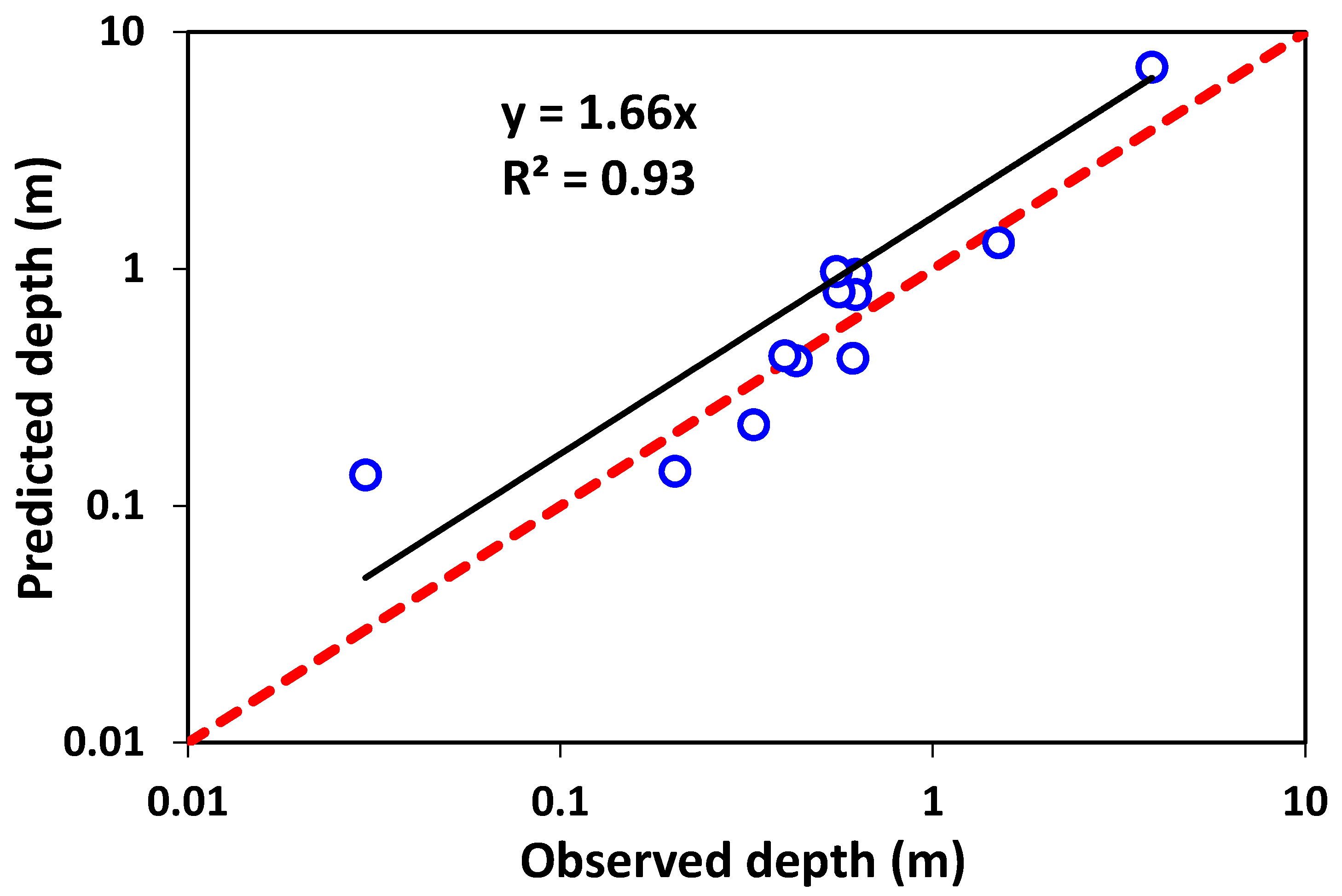
Figure 2.
Predicted and observed soil depth as a function of slope. The Norton and Smith data were digitized from Jenny [10], but extend only to a slope of 8 degrees. The Heimsath et al. [45] data were reported in a Table and extend over the range of 6 degrees to 32 degrees. The erosion function input was digitized from Figure 1 of Montgomery and Brandon [60]. I was given in Table 1 here, and a typical particle size of 30 μm, close to the 20 μm value considered to be most likely to characterize the San Gabriel mountain slopes, was applied. In order to reduce the scatter in the reported data, we give the mean soil depth at any particular slope value, although this will attach additional weight to the locations with deeper soils.

Table 1.
Predicted soil depths from reasonable infiltration and given erosion rates.
| Station | Region a | E (m/Myr) | I/φ b (m/yr) | P (m/yr) | Predicted c x (m) | Observed Mean x (m) | Reference Number d |
|---|---|---|---|---|---|---|---|
| Brown Mountain | AU | 14 | 0.22 | 0.69 | 0.95 | 0.62 | [35,49] |
| Frog’s Hollow1 | AU | 10 | 0.2 | 0.72 | 1.29 | 1.5 | [35,46,49] |
| Frog’s Hollow2 | AU | 27 | 0.2 | 0.72 | 0.41 | 0.43 | [35,46,49] |
| Snug | AU | 35 | 0.26 | 0.87 | 0.42 | 0.61 | [35,49] |
| Nunnock River | AU | 35 | 0.45 | 0.91 | 0.78 | 0.62 | [35,49] |
| Coos Bay | OR | 119 | 1.58 | 1.68 | 0.80 | 0.56 | [47,50] |
| Gongga Mountain | CH | 2500 | 0.78 | 1.95 | 0.14 | 0.203 | [43,51,52,53,54,55] |
| European Alps | EU | 127 | 0.55 | 1.55 | 0.22 | 0.33 | [44,56,57] |
| Tennessee Valley | N.CA | 35 | 0.7 | 0.92 | 0.43 | 0.4 | [39,48,50,58] |
| Merced River | C.CA | 13.75 | 0.1 | 0.31 | 7.12 | 3.87 | [42,50] |
| San Gabriel Mountain-west | S.CA | 35 | 0.55 | 0.81 | 0.65 to 1.3 | 0.55 | [45,50,59] |
| San Gabriel Mountain-east | S.CA | 200 | 0.55 | 0.81 | 0.09 to 0.18 | 0.03 | [45,50,59] |
Notes: a Region: AU = Australia, OR = Oregon, N. CA = North California, C. CA = Central California, S. CA = South California, CH = China, EU = Europe. b I = P − AET − Run-off. P, AET and Run-off rates used to calculate the infiltration rate in the United States were obtained from the Cal-adapt website [50], and in Australia, P values from Heimsath group [35], AET and Run-off values from the Bureau of Meteorology [49], P for Gongaga Mountain is from He et al. [43], AET was given by Gao et al. [51], given the fact that 80% of the total run-off from Gongga Mountain comes from glacial melting [54], 20% of run-off rates from Lin and Wang [55] was estimated as run-off lost from precipitation. For the European Alps, P is from Egli et al. [44], AET from the evapotranspiration map of Europe on the IMPACT2C web-atlas [56], run-off values from Wehren et al. [57]. Here we take φ = 0.4 as typical porosity. c For all data sets except Gongga Mountain and the 4 Californian sites, a typical particle size of 30 μm was chosen to calculate predicted depth, since no particle size data were reported. For Tennessee Valley, 10 μm was taken as x0, since most of the soils at Tennessee Valley fit into the clay loam category [58] with median particle size 10 μm [48]. He et al. [43] report a typical particle size of 400 μm for Gongga Mountain; White et al. [42] give 530 μm for Merced River; for San Gabriel Mountains, soils are mainly loams on the hillslopes [59], which has median particle size ranging from 20 to 40 μm. Here we take both values to obtain a range of soil depths in the San Gabriel Mountains.
Table 2.
Predicted steady-state soil depths for conditions reported by Montgomery [27].
Table 2.
Predicted steady-state soil depths for conditions reported by Montgomery [27].
| Status or Condition | <E> a (mm/yr) | Predicted Depth a (m) | Time a (yr) | E b (mm/yr) | Predicted Depth b (m) | Time b (yr) |
|---|---|---|---|---|---|---|
| Traditional agriculture | 3.934 | 0.0038 | 254 | 1.537 | 0.011 | 651 |
| Conservation agriculture | 0.124 | 0.21 | 8064 | 0.082 | 0.33 | 12,200 |
| Natural vegetation | 0.053 | 0.54 | 0.013 | 2.74 | ||
| Soil production c | 0.036 | 0.85 | 0.017 | 2.01 | ||
| Geological erosion | 0.173 | 0.14 | 0.029 | 1.09 | ||
| Mean soil depth d | 0.51 | 1.95 |
Notes: a <E> denotes mean erosion rates. Predicted depth is calculated using <E>, I = 0.5 m/year, and x0 = 0.00003 m. T is the corresponding time (approximate) to reach steady state starting form a soil depth of x = 1 m, T = x/<E>; b E denotes median erosion rates. Predicted depth is calculated using E, I = 0.5 m/year, and x0 = 0.00003 m. T is the corresponding time (approximate) to reach steady state starting form a soil depth of x = 1 m, T = x/E; c The rate is not an erosion rate, but the soil production rate, and the depth is the soil depth that would generate such a production rate; d Mean soil depth is calculated from averaging individual values in the column above it.
© 2017 by the authors. Licensee MDPI, Basel, Switzerland. This article is an open access article distributed under the terms and conditions of the Creative Commons Attribution (CC BY) license (http://creativecommons.org/licenses/by/4.0/).
Share and Cite
MDPI and ACS Style
Yu, F.; Faybishenko, B.; Hunt, A.; Ghanbarian, B. A Simple Model of the Variability of Soil Depths. Water 2017, 9, 460. https://doi.org/10.3390/w9070460
AMA Style
Yu F, Faybishenko B, Hunt A, Ghanbarian B. A Simple Model of the Variability of Soil Depths. Water. 2017; 9(7):460. https://doi.org/10.3390/w9070460
Chicago/Turabian StyleYu, Fang, Boris Faybishenko, Allen Hunt, and Behzad Ghanbarian. 2017. "A Simple Model of the Variability of Soil Depths" Water 9, no. 7: 460. https://doi.org/10.3390/w9070460
Note that from the first issue of 2016, this journal uses article numbers instead of page numbers. See further details here.