Economic and Energy Criteria for District Meter Areas Design of Water Distribution Networks

Abstract

Water Network Partitioning (WNP) improves water network management, simplifying the computation of water budgets and, consequently, allowing the identification and reduction of water losses. It is achieved by inserting flow meters and gate valves into a network which has been previously clustered into subsystems. Generally, the procedures are subdivided into two main steps: the clustering and partitioning phases. At first, network nodes are assigned to each cluster and then the appropriate pipes are selected, in which flow meters or gate valves are to be inserted. In this paper, an improved multilevel-recursive bisection algorithm was used to achieve network clustering. To better allocate the hydraulic devices, the partitioning phase was carried out through the minimization of a novel, multi-objective function, taking simultaneous account of energy and economic aspects. The aim is to define a solution that occupies a minimum possible number of flow meters, simplifying the water budget computation, preserving the hydraulic performances, and minimizing the capital and the operational costs. The procedure was tested on an extensive and real Mexican network, providing different optimal solutions and a smart Decision Support System (DSS) (based on visual diagrams and innovative energy, robustness, and balancing metrics).

1. Introduction

Nowadays, most systems have a networked structure (from the Internet to transportation, to food webs, as well as social and biochemical structures), making their dynamic behaviour and development difficult to understand. If—on the one hand—it makes network structures more robust against unplanned and unforeseen operational conditions [1], on the other hand it obligates the development of new analysis approaches to better understand their complex functioning. In recent years, the paradigm of “divide and conquer” has been adopted in order to simplify the management of water distribution systems, reducing the complexity of networks by subdividing them into more manageable sub-regions. The possibility of defining a community structure (i.e., the division of network nodes into groups, within which the network connections are dense but outside of which are sparse) is one of the most attractive properties of this approach. The ability to find and analyse such groups can provide invaluable help in understanding and visualising the structure and behaviour of the networks, making the identification of common and distinctive features simpler.

This strategy, introduced in 1980 in the UK and advised by the International Water Association [2], was useful and effective for Water Distribution Systems (WDSs) [3,4,5]. The core goal with this strategy is to achieve better control over the distribution of water [6]; however, there is an added benefit, in that it will permit the localization of water losses to be simplified [7]. Additionally, it allows for the application of pressure-management techniques [8] (such as the closure of some pipes which produces significant pressure drops and consequently mitigates background leakage [9]), enabling the identification of the most vulnerable areas [2]. In recent years, the combination of partitioning with the use of Pressure Reducing Valves has been investigated, as it has been shown to boost the efficiency of the pressure regulation provided by these devices [10]. Furthermore, WNP techniques have been proposed to protect network water quality against accidental or malicious contamination [11,12], using innovative water quality sensors [13] and parameter-estimation techniques [14].

For all these reasons, several methods and procedures for re-designing the existing WDS into sub-zones (called District Metered Areas (DMAs)) have been suggested in recent years, starting from empirical, trial-and-error procedures [11] to sophisticated, automated tools, integrating network analysis, graph and network theory, and optimization methods. Generally, the proposed procedures are arranged into two phases [15]: (1) the clustering and (2) the dividing steps. In the first phase, the shape and dimension of the network subsets are defined, based on different procedures that are intended to minimize the number of edge-cuts and to balance the number of nodes for each district (using graph algorithms [16,17,18], multilevel partitioning [19], community structure [20], or the spectral approach [21,22]). In the physical partitioning, the selection of pipes which are to have flow meters or gate valves inserted is carried out with an iterative [18] or optimization algorithm [23], with the purpose of defining the optimal layout that minimizes investment and the hydraulic deterioration [9].

In this paper, the definition of clusters was done through a multilevel-recursive bisection algorithm [24], opportunely suited for the WDS by Di Nardo et al. [25]. The novelty of the proposed procedure lies in the second phase of the partitioning procedure, in which the optimal device position was found through the minimization of a novel multi-objective function, taking into account hydraulic performances (the delivered power P_N) and the total costs (both initial and operating costs). This interaction is not well-studied yet; in fact, the proposed methodologies have these shortcomings: (i) the applicability is for small networks and not automatic [9]; (ii) the number of DMAs is not assigned as an input and the procedure is not arranged as a Decision Support System capable of comparing different optimal solutions using several indices [26].

In this work, the procedure was tested on an entire, all-pipe water network model of a large Mexican city, and it also provided a smart Decision Support System (DSS) based on quantitative measures and diagrams for evaluating the optimal layout (in terms of the number of DMAs). In this way, it was possible to find a partitioning layout that minimized investment costs and hydraulic deterioration, in compliance with water utilities requirements.

Another novel point of interest is the usage of some metrics based on complex network theory [27,28], which exploits the properties of the adjacency matrix to compare different WNP layouts that have already proven to be efficient for understanding, and describing the complex behaviour of WDSs [29,30]. The following is a description of these metrics and their meaning, which will serve to highlight the effectiveness of their usage.

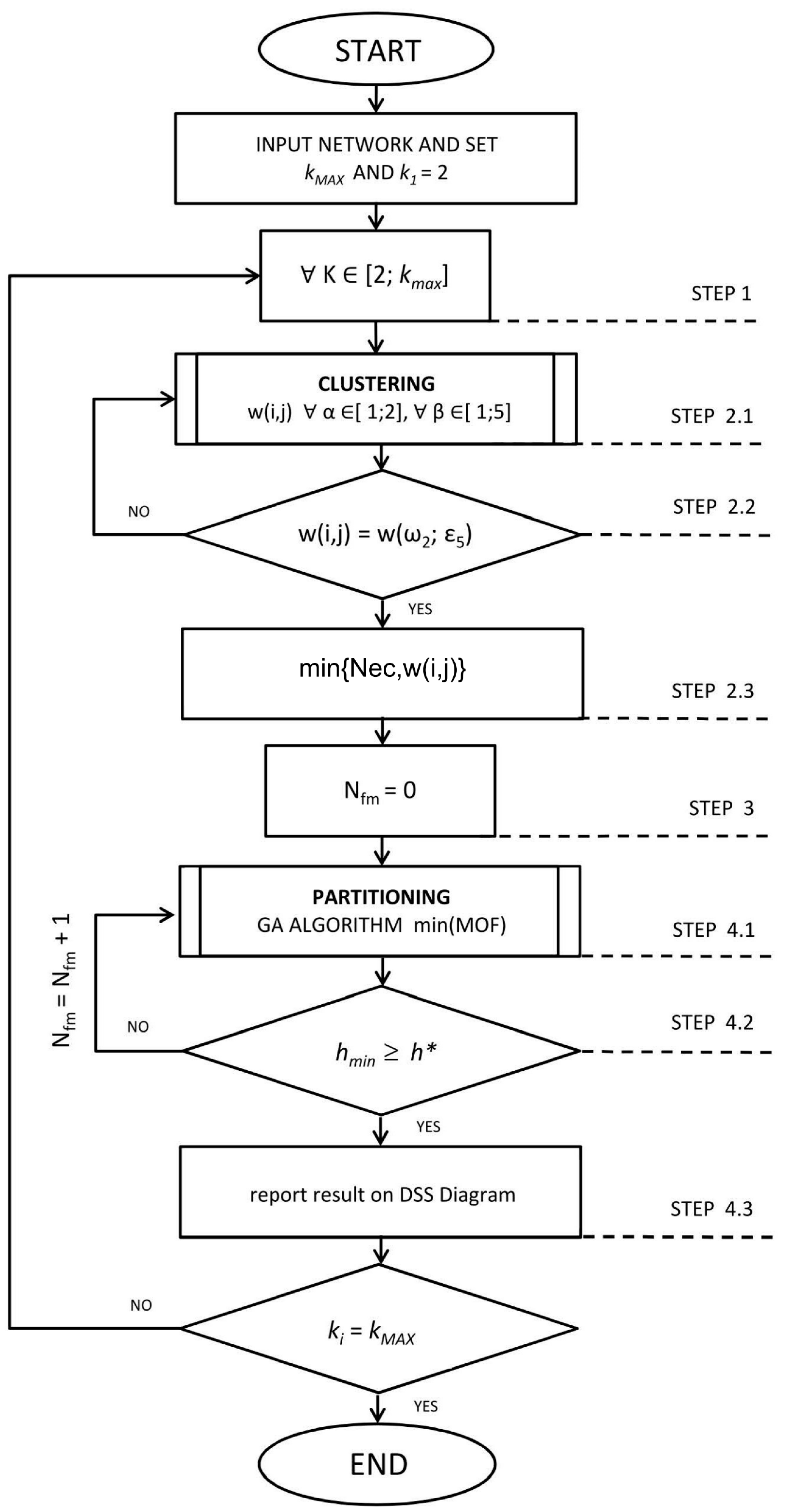
2. Decision Support System for Water Network Partitioning

The proposed methodology is illustrated in Figure 1, where the main steps needed to obtain the DSS diagrams are summarized (specifically, with reference to the main phases): (1) choice of the total number of districts, (2) clustering, (3) minimization of the number of flow meters, (4) partitioning and DSS diagram. It has proven to be an effective decision-making tool for water utility operators by enabling the selection of an optimal layout of DMAs.

The starting point for creating clusters (and then DMAs in a WDS) is to take all of the available network information into account. An effective strategy is to represent WDS as a particular graph, where the edges are pipes and the nodes are junctions and consumption points—this defines the structure of the graph from a geographical and connectivity point of view [31]. In this regard, a WDS can be considered as a simple graph G = (V,E) (where V is the set of n vertices (or nodes) and E is the set of m edges (or links)), or, as a weighted graph (if some vertices or edges have associated weights indicated respectively with ωαi (e.g., demand, elevation, etc.), for i = 1…n, or with εβl (length, diameter, flow, dissipated power, etc.), for l = 1…m). The required information is easily available from water utilities, and through the use of hydraulic simulation software such as EPANET [32]. According to this schematization, the clustering phase was carried out with a multilevel-recursive bisection algorithm, as described below.

As reported in the flow-chart, in STEP 1 the topological and hydraulic characteristics of the network are provided to the SWANP 2.0 software (Aversa, Italy) [25]: network characteristics (i.e., pipe diameters and lengths; nodal water demands; reservoir or tank heads), number and position of hydraulic devices (i.e., valves and pumps), initial and maximum number of DMAs (k₁ = 2; k_max), and network design pressure h^*. The SWANP 2.0 software allows to design of the optimal water network partitioning (both the clustering and the partitioning phase), comparing different layouts with some hydraulic, topological, and protection performance indices (based on several multi-objective functions). STEP 2 consists of clustering the water network in k_i sub-zones (or clusters), in such a way that each node I $\in$ V belongs uniquely to one of the clusters k₁, k₂, ..., k_max, k_i ∩ k_j = 0, for i ≠ j, and ∪_ik_i = V. In this paper, a novel aspect is that network clustering was carried out using an improved version of the multilevel-recursive bisection algorithm [25], which takes different hydraulic weights into account for both the nodes and the edges (in order to define which of them provides the best cluster layout, simultaneously minimising the total number of edge-cuts N_ec between clusters and balancing the number of nodes in each cluster).

In this regard, at STEP 2.1 the weight matrix W—reported in

Table 1. Weight matrix W composed of vertex-edge weight combinations ω_α and ε_β.

	ε1j (No Weight)	ε2j (Flow)	ε3j (Diameter)	ε4j (Length)	ε5j (Dis. Power)
ω1j (No weight)	w(1,1)	w(1,2)	w(1,3)	w(1,4)	w(1,5)
ω2j (demand)	w(2,1)	w(2,2)	w(2,3)	w(2,4)	w(2,5)

—was defined; each element w(i,j) is a vertex-edge weight combination of (ω_α, ε_β). In particular, the following weights were used: α = 1, 2 and β = 1,…, 5: ω₁ = No weight, ω₂ = Demand, ε₁ = No weight, ε₂ = Flow, ε₃ = Diameter, ε₄ = Length and ε₅ = Dissipated Power. Specifically, the last one is described by Equation (1):

$$P_D= \gamma .{{\displaystyle \sum }}_{j=1}^m\Delta H_j·q_j$$

(1)

where γ is the specific weight of water, $\Delta H_j$ and $q_j$ are respectively the head loss and the flow in the j-th pipe. For example, without loss of generality (as shown in Table 1), the weight combination w(2,3) = (ω₂,ε₃) = (Demand, Diameter) assigns the demand (as weight at each node) and the diameter (at each pipe).

In the STEP 2.1-STEP 2.3 cycle, SWANP 2.0 analyses all ten weight combinations w(i,j) of the matrix W (from w(1,1) to w(2,5) [25]), in order to find which of them minimizes the number of edge-cuts (min{N_ec,w(i,j)}) and balances the clusters.

Once the optimal layout is defined in the clustering phase, it becomes the starting point for the subsequent partitioning phase. Another point of novelty is that, in this phase, the aim is to minimize the constrained multi-objective function (MOF) (1), finding the optimal devices positioning (gate valves N_bv and flow meters N_fm = (N_ec − N_bv)) and, simultaneously, inserting the minimum number of flow meters (STEP 3) in order to simplify the water budget and pressure control. In this paper, the approach known as the “weighted-sum” or “scalarization” method [33] was adopted which allows for the definition of a new optimization problem with a unique objective function, made up of two or more functions:

$$MOF= \left(y_1 + y_2 + y_3\right)$$

(2)

$$y_1=\frac{C_{fm}+C_{bv}}{C^{*}}$$

(3)

$$y_2=\frac{C_E}{C_E^{*}}$$

(4)

$$y_3=1-\frac{P_N}{P_N^{*}}$$

(5)

where C_fm and C_bv are the costs (dependent on the pipe diameter where they will be installed) of the flow-meters and gate valves, respectively; C* is the total cost of devices computed by inserting the N_fm flow meters into boundary pipes (with the maximum diameter) and the N_bv gate valves on the rest of boundary pipes; and C_E is the energy cost of all the pumping stations in the partitioned network layout, computed as:

$$C_E=c·\Delta t·\gamma {\displaystyle \sum }_{j=1}^{n_{pump}}{q}_j{H}_j$$

(6)

with c the unit energy cost, Δt the time operational interval, γ the specific weight of the water, q_j and H_j the flow and the hydraulic head of the j-th pump, and n_pump the total number of pumps; C^*_E is the corresponding value of energy consumed by the original network layout; and P_N is the total node power computed for the partitioned network.

$$P_N=\gamma {\displaystyle \sum }_{i=1}^n{Q}_i{H}_i$$

(7)

where Q_i and H_i are the water demand and hydraulic head of the i-th node, and P^*_N is the corresponding value of the original network layout.

Further, the MOF is constrained by the following expression, which imposes a minimum service level for the users:

$$constraint=\left(h_{min}\ge h^{*}\right)$$

(8)

where h_min is the minimum nodal pressure head and h^* is the network design pressure. Starting from the solution with N_fm = 0 (only gate valves inserted in all the boundary pipes), if the constraint is not fulfilled in STEP 4.2, it assigns N_fm = 1 and SWANP 2.0 finds the solution that minimizes the MOF (repeating STEP 4.1 and increasing by one the number of flow meters until the constraint (8) is fulfilled).

It is important to emphasize that the partitioning phase required an optimization procedure to find the best solution. Indeed, the number of possible layout combinations, N_ck, (i.e., the number of all possible ways in which to place the hydraulic devices) is so huge that it is computationally impossible to investigate all the space solutions. To overcome this problem, a Genetic Algorithm (GA) is adopted in this paper to find an optimal solution [25] with the novel constrained MOF (2).

Finally, in STEP 4.3 (for each k_i), the proposed procedure provides simulation results in terms of: (a) WNP layout with optimal positioning of boundary valves and flow meters; and (b) a DSS diagram with the corresponding capitalized optimal cost, computed through the formula of capitalization:

$$C_t^{\prime }=C{\left(1+r\right)}^t$$

(9)

where C’_t is the future capital after t years, C is the actual cost, and r is the capitalization rate. In the present work, the time interval t = 20 was chosen (according to an average lifetime of devices and an average time of an economic investment for a water utility), while the capitalization rate was r = 6%.

Once the DSS diagram is completed, and the maximum available budget C’_tot,max is set, the operator can choose the optimal district layout by consulting a battery of performance indices provided as additional criteria (reported in Table 5). In particular, Table 5 shows: the (a) hydraulic indices: mean h_mean and minimum h_min node pressure, resilience index I_r [34] and resilience deviation I_rd; (b) topological indices: the Efficiency E_f (the measure of the traffic capacity of a network, as function of the mean of separation between each node), the Algebraic connectivity λ₂ (the second smallest eigenvalue of the Laplacian matrix, which expresses the strength of dividing into sub-regions), and the zero eigenvalue multiplicity m_a (equal to the number of connected components in a network [35] used to establish if the dividing phase generated isolated sub-regions, which is not a preferable solution for the preservation and continuity of the system). Finally, the standard deviations are SD_nc and SD_l (of the number of service connections of each district n_ck, and of the length of each district l_k, respectively), which can be assumed as measures of the topological balancing of the partitioning (lower values indicate districts more similar in size).

The DSS diagram defines a range of optimal partitioning solutions so that, through the performance indices along with the consideration of topological aspects, it becomes possible to select the best number of districts. In this way, the proposed procedure offers a heuristic methodology to finding an optimal solution to the arduous problem of defining a water network partitioning (with a more “user friendly” approach based on simple-decision-support-system diagrams, and on a battery of performance indices capable of taking energy, economic, and topological criteria into account simultaneously).

3. Results and Discussion

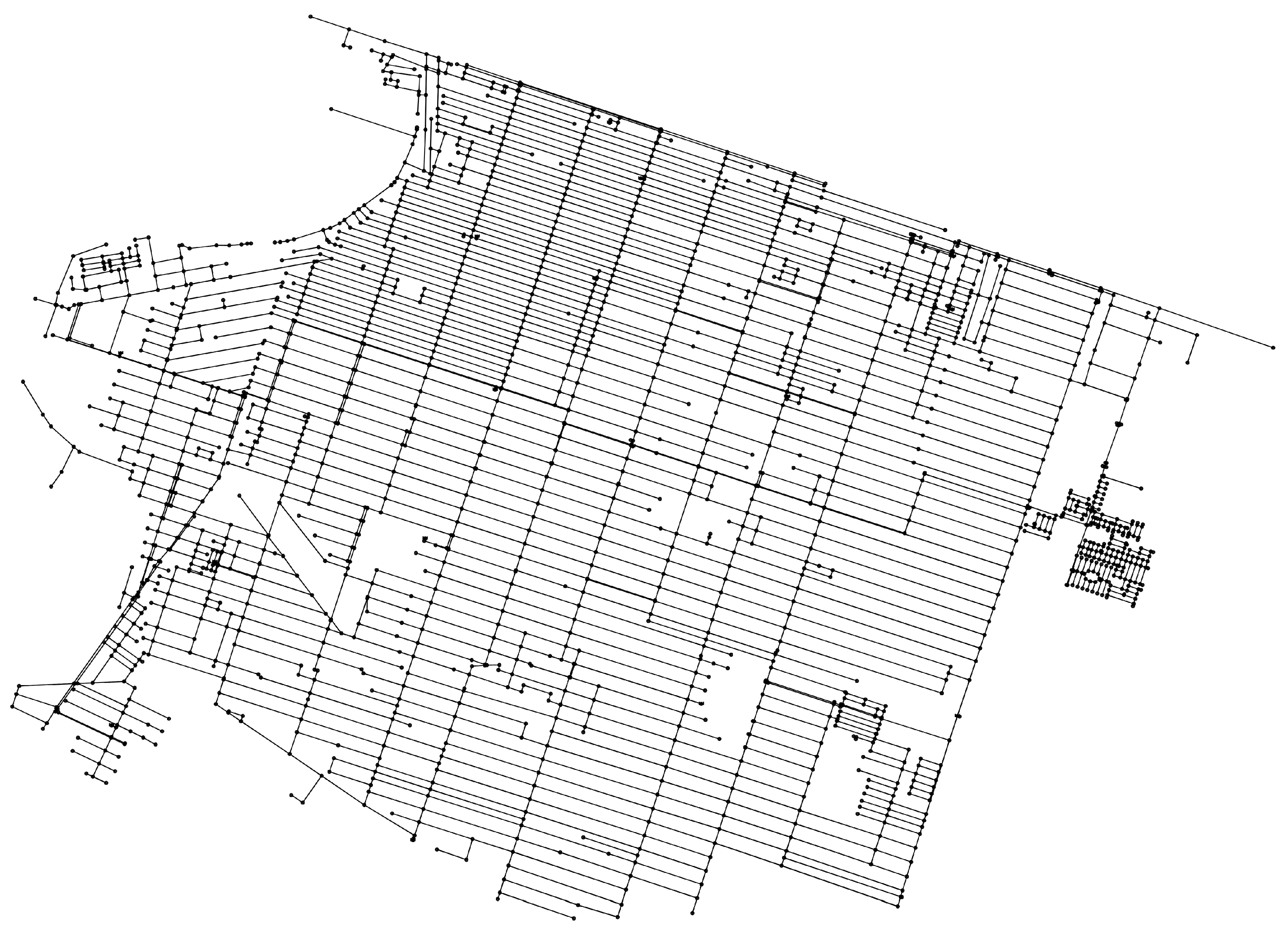
3.1. Case Study

The effectiveness of the proposed methodology was tested on the real case study of San Luis Rio Colorado (Figure 2), a large network in Mexico [36]. San Luis Rio Colorado is a Mexican city located in the northern part of the state of Sonora, which is near the Mexico-United States (US) border. The network serves approximately 180,000 citizens, through a total of 48,400 service connections (45,850 of which are residential, 2445 of which are commercial, and 105 of which industrial). The distribution network is approximately 50 years old, composed of 60-mm to 500-mm asbestos cement and plastic (polyvinyl chloride, PVC) pipes. The water supply sources consist of 18 deep water wells, fully interconnected by the distribution network at the beginning of the partitioning project, and which do not have water tanks. Some of the well pumps are equipped with variable speed drives that allow the pumps to follow water demand variation and stop them when water demand is very low. The main characteristics of the hydraulic model for the network are reported in

Table 2. Main characteristics of the San Luis Rio Colorado network.

Characteristic	Value
Number of nodes n	1890
Number of links m	2681
Number of wells w	18
Number of service connections ncTOT	48,400
Head of well pumps [m]	−2.00; −8.87; −6.45; −2.85; −9.38; −0.75; −4.10; −7.23; 0.05; 0.62; −3.19; −3.80; 3.55; 2.43; −7.32; −3.71; 1.85; 3.73
Total pipe length lTOT [km]	599.1
Minimum ground elevation zMIN [m]	0.00
Maximum ground elevation zMAX [m]	40.10
Pipe materials	PVC and AC
Pipe diameters [mm]	60; 62.5; 75; 100; 150; 200; 250; 300; 350; 400; 450; 500
Average demand. Q [L/s]	1127.92
Peak demand Q [L/s]	1735.26
Design pressure h* [m]	12.00
Unit energy cost c [€/kWh]	0.09

; in this regard, based on local standards design, the design pressure h^* = 12 m.

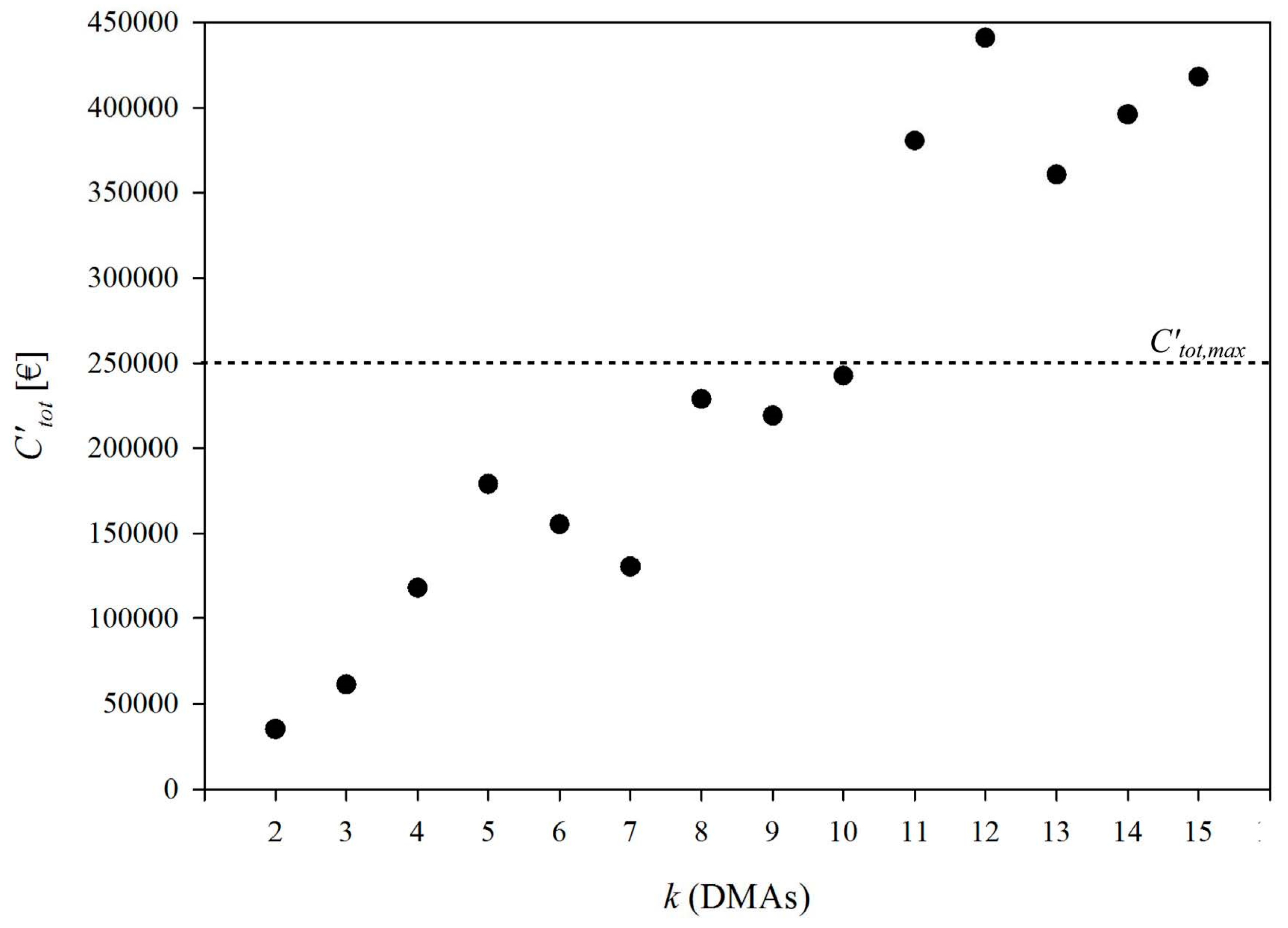
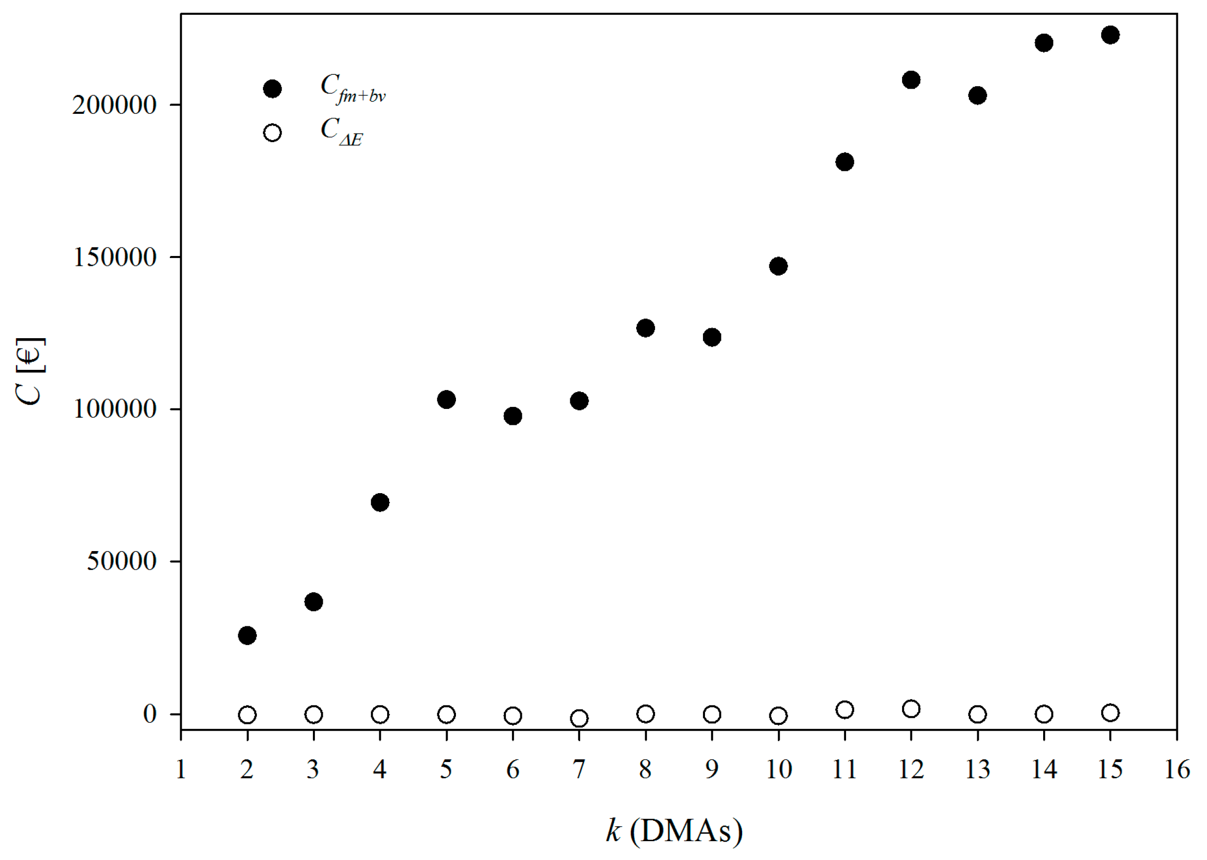
3.2. Assessment Results of the Multi-Objective Function

The hydraulic simulations were conducted with a Demand Driven Approach; considering peak water demand in summer, this is the worst condition for the Mexican water networks, since (generally) they are not designed for fire-fighting conditions. After an extensive cost analysis of gate valves and flow meters, in

Table 3. Cost of devices in function of pipe diameter.

Pipe Diameter [mm]	Flow Meter Cost [€]	Gate Valve Cost [€]
50	1974	520
65	2073	560
80	2073	592
100	2187	676
125	2325	784
150	2586	940
200	2970	1232
250	3990	1792
300	5109	2228
350	5652	3242
400	6282	4412
450	6726	5964
500	7125	9122
600	8265	11,406
700	10,599	15,578
800	12,909	21,177
900	16,011	27,198
1000	19,353	33,989

the average cost of each device is reported according to the pipe diameter.

In

Table 4. The San Luis Rio Colorado network simulation results for k = 1 to k = 15 DMAs.

k [-]	Nck [-]	Nec [-]	Nfm [-]	Nbv [-]	PN [W]	MOF [-]	Cfm+gv [€]	CΔE [€/Year]	C’tot [€]
1	-	-	-	-	104,936.44	-	-	-	-
2	1	16	0	16	101,962.58	2.01	25,726.13	−281.08	35,111.68
3	1	26	0	26	101,365.40	2.02	36,733.56	−120.03	61,103.94
4	1,533,939	47	5	42	102,831.98	2.01	69,377.52	−156.16	118155.32
5	61,474,519	62	9	53	102,863.55	2.02	103,115.38	−147.33	178,919.18
6	6.52 × 1013	67	8	59	100,619.71	2.03	97,803.87	−505.03	155,459.53
7	1.47 × 1013	72	7	65	102,156.07	2.01	102,763.27	−1373.63	130,471.94
8	1.80 × 1020	85	17	68	104,206.23	1.99	126,708.65	44.73	228,660.08
9	3.53 × 1019	77	15	62	104,767.04	1.01	123,656.96	−65.85	218,883.30
10	3.15 × 1021	92	16	76	104,560.70	2.01	146,992.26	−530.07	242,571.74
11	2.16 × 1028	108	26	82	104,216.64	1.01	181,208.25	1435.99	380,509.48
12	2.98 × 1031	122	28	94	102,889.14	1.03	208,214.42	1744.91	440,918.92
13	4.75 × 1031	129	29	100	103,304.48	2.01	203,090.31	−86.48	360,331.58
14	7.19 × 1032	135	30	105	101,905.98	1.04	220,366.52	36.12	396,051.14
15	5.42 × 1033	138	31	107	102,555.23	2.03	222,936.65	486.62	418,220.20

(for each optimal WNP layout), the following data are reported: the number k of DMAs, the total number of possible combinations of device locations N_ck, the number of edge-cuts N_ec, the number of flow meters N_fm and gate valves N_bv, the total delivered power P_N and the value of MOF, the total cost of devices C_fm+gv = C_fm + C_gv, the difference of energy cost C_ΔE (computed comparing the energy cost of the original layout without partitioning, and of the WNP layout (and referring to the year of device installation)) and, finally, in the last column of Table 4, the total capitalized cost C’_tot = C’_ΔE + C’_fm+gv, where C’_ΔE is the capitalized cost of energy and C’_fm+gv is the capitalized cost of devices.

It is worth highlighting that, at first (from k =2 to k = 4), the total number of possible combinations of device locations is low, and so it is possible to find the best solutions that minimize MOF (1), investigating the entire solution space. From k = 5 to k = 15 DMAs the number of possible combinations N_ck (from N_c5 = 61,474,519 to N_c15 = 5.42 × 10³³) is so huge that it becomes computationally impossible to analyse all possible configurations and, for this reason, an optimal (but maybe not the absolute best) solution is found with a genetic algorithm (GA). Through the use of a heuristic optimisation method (minimising the multi-objective function), the optimal position of devices on the boundaries is found. The GA simulations were computed using 100 generations, with a population consisting of 500 individuals and a crossover percentage equal to P_cross = 0.8 (and without termination criteria).

From Table 4 it is clear that the number of edge-cuts, and thus, the number of gate-valves and flow-meters (and as a consequence the total cost of the devices C_fm+gv), grows almost linearly with the number of DMAs. It is interesting to note that for some WNP layouts, the annual cost of energy decreases, so these DMA configurations lead to money saving, with a maximum decrease of C_ΔE = −1373.63 €/year (for k = 7 DMAs). This is a very interesting result, and it is due to the insertion of gate valves (which reduce nodal pressures and, consequently, decrease the energy required by the pumping stations, while meeting the minimum level of service for the users (nodal pressures closer to design pressure h^*)). As shown in Table 4, for the WNP layouts with k = 2 and k = 3, the optimal solutions provide only gate valves on all boundary pipes, and so the DMAs are completely isolated from each other; all the same, the 12 m pressure constraint at each node is maintained. The total cost of devices C_fm+gv and the difference of the annual energy cost C_ΔE are reported in the Figure 3.

As shown, the yearly variability of C_ΔE is negligible compared to the total devices cost, which grows almost linearly with the number of districts. In Figure 4, the capitalized total cost C’_tot is reported for each WNP layout, from k = 1 to k = 15 DMAs.

Figure 4 shows that the capitalized total cost, although with a growing trend as expected, does not grow linearly with the number of districts. This is because: (a) the number of the edge-cuts (see Table 4) does not grow uniformly; (b) the device cost does not increase linearly with the diameter of pipes on which they are installed; (c) the flow-meters cost is different from the gate-valves cost; (d) the solutions found by the GA are sub-optimal (not the best) because, as explained above, it is computationally impossible to investigate all possible combinations; (e) the clustering phase, as already highlighted in a previous study [37], can provide DMA layouts which are not optimal for the subsequent partitioning phase (most of all in the case with many water sources); and (f) some WNP layouts, as already explained in the paper, require lower total energy, providing energy cost savings that are subtracted from the cost of devices. These considerations, coming from the complexity of the non-linear problem of the water partitioning design, show some very interesting aspects for water utilities because, with a heuristic optimization approach, it is possible to find some layouts that have a larger number of DMAs (but they can have a lower total investment cost).

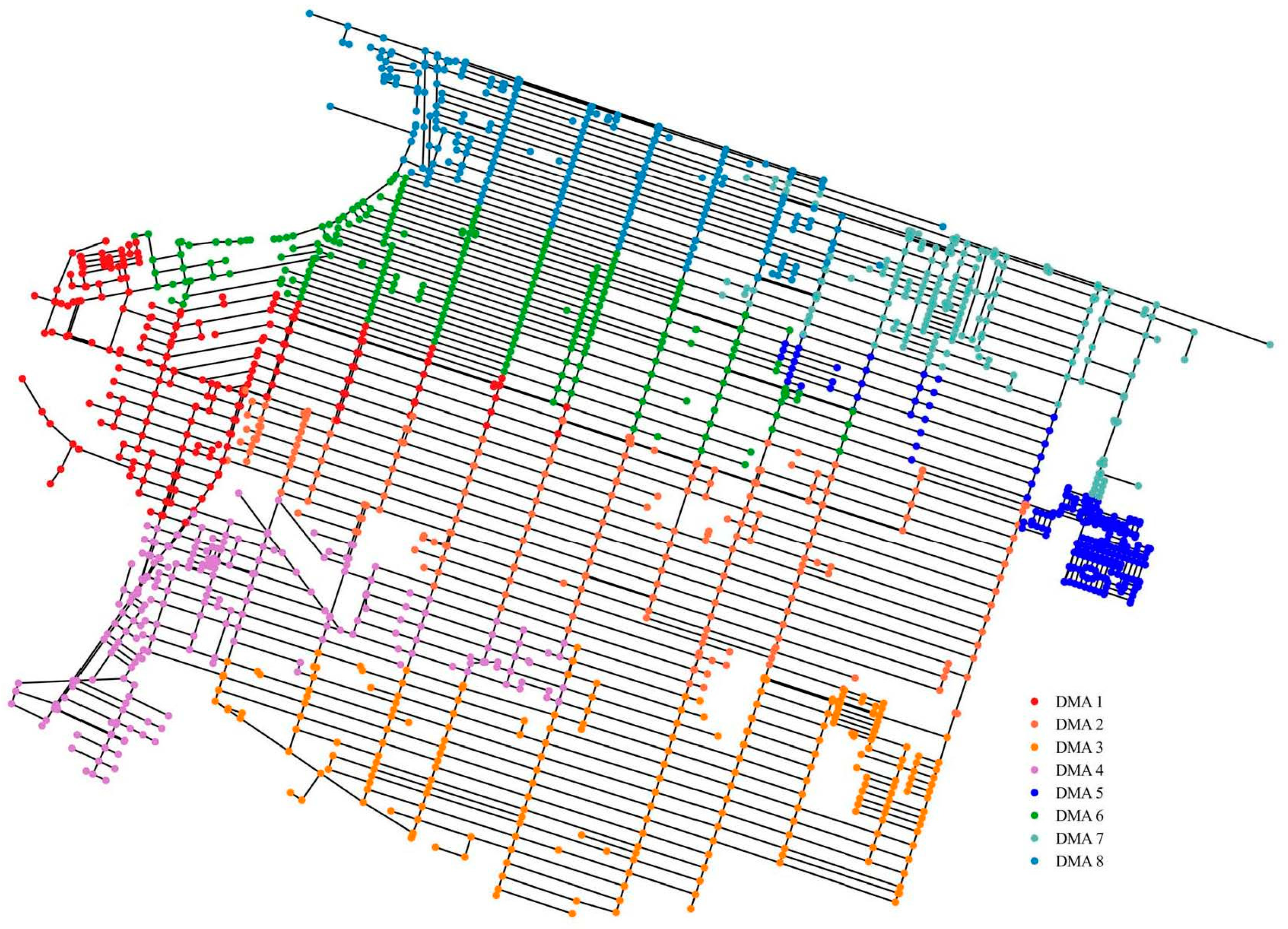
3.3. Assessment Results of Hydraulic and Topological Performance Indices

In

Table 5. Hydraulic and topological performance indices.

k [-]	hmean [m]	hmin [m]	Ir [-]	Ird [%]	Ef [W]	λ2 [-]	mα [-]	SDnc [-]	SDl [-]
1	26.63	16.31	0.803	0.00	0.0520	0.0009	1	-	-
2	26.63	13.42	0.710	11.58	0.0366	0.0000	2	1.43	0.16
3	25.58	13.92	0.722	10.09	0.0343	0.0000	3	0.72	2.11
4	25.93	15.26	0.750	6.60	0.0458	0.0004	1	6.31	6.25
5	26.10	15.15	0.763	4.98	0.0464	0.0003	1	0.45	1.15
6	25.69	12.96	0.690	14.07	0.0330	0.0000	2	6.75	5.93
7	26.07	14.93	0.759	5.48	0.0383	0.0000	2	5.51	5.52
8	27.00	14.75	0.764	4.86	0.0457	0.0005	1	5.15	4.77
9	27.91	12.56	0.761	5.23	0.0384	0.0000	2	4.32	4.64
10	27.42	12.12	0.765	4.73	0.0348	0.0000	2	4.68	4.39
11	26.99	12.60	0.736	8.34	0.0440	0.0003	1	3.69	3.51
12	26.38	12.01	0.701	12.70	0.0425	0.0003	1	3.79	3.56
13	26.75	15.37	0.734	8.59	0.0443	0.0005	1	3.31	3.09
14	26.49	13.02	0.667	16.94	0.0444	0.0004	1	0.11	0.13
15	26.85	15.01	0.698	13.08	0.0431	0.0005	1	0.13	1.07

, the hydraulic and topological performance indices are reported, in order to evaluate the potential deterioration under partitioning for each WNP layout. This provides further decisional tools that take other important technical characteristics into account. The mean and minimum pressures of all WNP layouts are close to their original values, showing that the partitioning provides only a slight hydraulic deterioration (confirmed, also, by the small alteration of the resilience index, which attains its maximum deterioration value for k = 14 DMAs, with I_rd = 16.94%).

From the topological point of view, the efficiency E_f attains lower values for the WNP layouts which disconnect the network (with k = 2, 3, 6, 7, 9 and 10 DMAs), and so they have worse nodal “communications”. The minimum value E_f = 0.0330 corresponds to k = 6 DMAs. For the same WNP layouts, the algebraic connectivity λ₂ is zero. The lower λ₂ is, the more sensitive the network is to the efforts of cutting it into sub-graphs, and thus the lower its robustness. In this regard, the best WNP layouts are for k = 8, 13, 15 DMAs, with λ₂ = 0.0005. The multiplicity m_α (of the zero eigenvalue of the Laplacian matrix) is equal to the number of connected sub-graphs in a network [38]. As shown in the corresponding column of Table 5, only the WNP layouts with k = 4, 5, 8, 11, 12, 13, 14 and 15 DMAs conserve the network continuity after partitioning, consequently showing a significantly higher topological robustness. Finally, the SD_nc and SD_l values show that all the solutions provide very balanced layouts (in terms of number of nodes and total length of the clusters, with the minimum values SD_nc = 0.11 and SD_l = 0.13 corresponding to k = 14 DMAs).

In Figure 4 an example of DSS application is reported. Fixed maximum budget C’_tot,max = 250,000$ (horizontal dashed line) WNP layouts from k = 11 to k = 15 DMAs are economically incompatible with the maximum available investment. The choice is reduced to WNP layouts from k = 2 to k = 10 DMAs. To arrive at the best choice, this order can be followed: (a) layout without disconnection (with m_α = 1), so the choice is reduced to k = 4, 5 and 8 DMAs; and then (b) low alteration of energy resilience I_r or higher values of robustness or most balanced districts, according to the requirements of operators.

Finally, in Figure 5 the WNP with 8 DMAs is illustrated.

4. Conclusions

The problem of designing an optimal water network partitioning is very complex because the number of possible layouts is huge, and also because it involves hydraulic, topological, and economic aspects. The proposed methodology can be used as a possible way to overcome the traditional empirical approaches, providing a decision support system based on a heuristic optimization approach (joining the technical and economic aims of water utilities interested in applying WNP).

The proposed procedure permits optimal partitioning of water supply networks by employing SWANP 2.0 software (which integrates some innovative partitioning algorithms, heuristic optimization techniques, and hydraulic and robustness metrics with a novel multi-objective function based on hydraulics, investment and operational costs). The novelties of the procedure consist, essentially, in taking into account both investment and energy costs, and total node power, for the definition of the optimal device position. Furthermore, the procedure provides a useful tool for water utilities (tested on a real, large WDS) to choose the optimal water network partitioning, based on innovative performance indices (some of them borrowed from complex networks theory, which allow the possibility of taking into account specific WDS’ topological aspects). The simulation results for the large water network in Mexico showed good results obtained with the MOF, even with a space solution of k = 15 DMAs (so large that it required a heuristic optimization procedure, based on a genetic algorithm). Once the maximum number of DMAs, the minimum value of nodal pressure, and the investment budget are defined, the procedure provides a “user friendly” DSS diagram to choose the optimal layout of water network partitioning (in terms of cost and technical performance, using different priority criteria). The impact of the research outcome could be improved by testing the DSS on other case studies. Further works will be oriented to the implementation of other clustering and dividing algorithms also using other economical metrics.

References

1. Estrada, E. Network robustness to targeted attacks. The interplay of expansibility and degree distribution. Eur. Phys. J. B 2006, 52, 563–574. [Google Scholar] [CrossRef]
2. Morrison, J.; Tooms, S.; Rogers, D. District Metered Areas: Guidance notes. In IWA Water Loss Task Force; IWA Publishing: London, UK, 2007. [Google Scholar]
3. Gomes, R.; Marques, A.; Sousa, J. Decision support system to divide a large network into suitable District Metered Areas. Water Sci. Technol. 2012, 65, 1667–1675. [Google Scholar] [CrossRef] [PubMed]
4. Alvisi, S.; Franchini, M. A heuristic procedure for the automatic creation of district metered areas in water distribution systems. Urban Water 2014, 11, 137–159. [Google Scholar] [CrossRef]
5. Di Nardo, A.; Di Natale, M.; Santonastaso, G.F.; Tzatchkov, V.G.; Alcocer-Yamanaka, V.H. Divide and conquer partitioning techniques for smart water networks. Procedia Eng. 2014, 89, 1176–1183. [Google Scholar] [CrossRef]
6. Chambers, K.; Creasey, J.; Forbes, J. Design and operation of distribution networks. In Safe Piped Water: Managing Microbial Water Quality in Piped Distribution Systems; Ainsworth, R., Ed.; IWA Publishing: London, UK, 2004. [Google Scholar]
7. Kunkel, G. Committee report: Applying worldwide BMPs in water loss control. J. Am. Water Work. Assoc. 2003, 95, 65–79. [Google Scholar]
8. De Paola, F.; Fontana, N.; Galdiero, E.; Giugni, M.; Savic, D.; Sorgenti degli Uberti, G. Automatic multi-objective sectorization of a water distribution network. Procedia Eng. 2014, 89, 1200–1207. [Google Scholar] [CrossRef]
9. Galdiero, E.; De Paola, F.; Fontana, N.; Giugni, M.; Savic, D. Decision Support System for the optimal design of District Metered Areas. J. Hydroinform. 2015, 18, 49–61. [Google Scholar] [CrossRef]
10. Creaco, E.; Pezzinga, G. Multiobjective Optimization of Pipe Replacements and Control Valve Installations for Leakage Attenuation in Water Distribution Networks. J. Water Resour. Plan. Manag. 2014, 141, 04014059. [Google Scholar] [CrossRef]
11. Grayman, W.M.; Murray, R.; Savic, D. Effects of redesign of water systems for security and water quality factors. In Proceedings of the World Environmental and Water Resources Congress, Kansas City, MO, USA, 17–21 May 2009; pp. 1–11. [Google Scholar]
12. Di Nardo, A.; Di Natale, M.; Musmarra, D.; Santonastaso, G.F.; Tzatchkov, V.; Alcocer-Yamanaka, V.H. Dual-use value of network partitioning for water system management and protection from malicious contamination. J. Hydroinform. 2015, 17, 361–376. [Google Scholar] [CrossRef]
13. Ostfeld, A.; Salomons, E. Optimal early warning monitoring system layout for water networks security: Inclusion of sensors sensitivities and response delays. Civ. Eng. Environ. Syst. 2005, 22, 151–169. [Google Scholar] [CrossRef]
14. Pasha, M.F.K.; Lansey, K. Water quality parameter estimation for water distribution systems. Civ. Eng. Environ. Syst. 2009, 26, 231–248. [Google Scholar] [CrossRef]
15. Perelman, L.S.; Allen, M.; Preis, A.; Iqbal, M.; Whittle, A.J. Automated sub-zoning of water distribution systems. Environ. Model. Softw. 2015, 65, 1–14. [Google Scholar] [CrossRef]
16. Deuerlein, J.W. Decomposition model of a general water supply network graph. J. Hydraul. Eng. 2008, 134, 822–832. [Google Scholar] [CrossRef]
17. Perelman, L.; Ostfeld, A. Topological clustering for water distribution systems analysis. Environ. Model. Softw. 2011, 26, 969–972. [Google Scholar] [CrossRef]
18. Ferrari, G.; Savic, D.; Becciu, G. Graph-theoretic approach and sound engineering principles for design of district metered areas. J. Water Resour. Plann. Manag. 2014, 140, 04014036. [Google Scholar] [CrossRef]
19. Izquierdo, J.; Herrera, M.; Montalvo, I.; Perez-Garcia, R. Division of Water Distribution Systems into District Metered Areas Using a Multi-Agent Based Approach. Commun. Comput. Inf. Sci. 2011, 50, 167–180. [Google Scholar]
20. Diao, K.; Zhou, Y.; Rauch, W. Automated creation of district metered area boundaries in water distribution systems. J. Water Resour. Plan. Manag. 2013, 139, 184–190. [Google Scholar] [CrossRef]
21. Herrera, M.; Canu, S.; Karatzoglou, A.; Perez-Garcia, R.; Izquierdo, J. An Approach to Water Supply Clusters by Semi-Supervised Learning. In Proceedings of the International Environmental Modelling and Software Society (iEMSs), Ottawa, ON, Canada, 5–8 July 2011; Swayne, D.A., Yang, W., Voinov, A., Rizzoli, A., Filatova, T., Eds.; pp. 1925–1932. [Google Scholar]
22. Di Nardo, A.; Di Natale, M.; Giudicianni, C.; Greco, R.; Santonastaso, G.F. Water supply network partitioning based on weighted spectral clustering. In International Workshop on Complex Networks and their Applications; Springer International Publishing: Warsaw, Poland, 2016; Volume 693, pp. 797–807. [Google Scholar]
23. Alvisi, S. A New Procedure for Optimal Design of District Metered Areas Based on the Multilevel Balancing and Refinement Algorithm. Water Resour. Manag. 2015, 29, 4397–4409. [Google Scholar] [CrossRef]
24. Karypis, G.; Kumar, V. Multilevel k-way partitioning scheme for irregular graphs. J. Parallel Distrib. Comput. 1998, 48, 96–129. [Google Scholar] [CrossRef]
25. Di Nardo, A.; Di Natale, M.; Santonastaso, G.F.; Venticinque, S. An automated tool for smart water network partitioning. Water Resour. Manag. 2013, 27, 4493–4508. [Google Scholar] [CrossRef]
26. Campbell, E.; Izquierdo, J.; Montalvo, I.; Pérez-García, R. A Novel Water Supply Network Sectorization Methodology Based on a Complete Economic Analysis, Including Uncertainties. Water 2016, 8, 179. [Google Scholar] [CrossRef]
27. Watts, D.; Strogatz, S. Collective Dynamics of Small World Networks. Nature 1998, 393, 440–442. [Google Scholar] [CrossRef] [PubMed]
28. Barabasi, A.L.; Albert, R. The Emergence of Scaling in Random Networks. Science 1999, 286, 797–817. [Google Scholar]
29. Yazdani, A.; Jeffrey, P. Complex network analysis of water distribution systems. Chaos: Interdiscip. J. Nonlinear Sci. 2011, 21, 016111. [Google Scholar] [CrossRef] [PubMed]
30. Di Nardo, A.; Di Natale, M.; Giudicianni, C.; Musmarra, D.; Santonastaso, G.F.; Simone, A. Water distribution system clustering and partitioning based on social network algorithms. Procedia Eng. 2015, 119, 196–205. [Google Scholar] [CrossRef]
31. Fernández, A.M.H. Improving Water Network Management by Efficient Division into Supply Clusters. Ph.D. Thesis, Universitat Politécnica de Valencia, Valencia, Spain, 2011. [Google Scholar]
32. Rossman, L.A. EPANET2 Users Manual; US E.P.A.: Cincinnati, OH, USA, 2000. [Google Scholar]
33. Caramia, M.; Dell’Olmo, P. Multi-Objective Management in Freight Logistic; Springer: Berlin, Germany, 2008. [Google Scholar]
34. Todini, E. Looped water distribution networks design using a resilience index based heuristic approach. Urban Water 2000, 2, 115–122. [Google Scholar] [CrossRef]
35. Boccaletti, S.; Latora, V.; Moreno, Y.; Chavez, M.; Hwanga, D.U. Complex networks: Structure and dynamics. Phys. Rep. 2006, 424, 175–308. [Google Scholar] [CrossRef]
36. Tzatchkov, V.G.; Alcocer-Yamanaka, V.H.; Rodriguez-Varela, J.M. Water Distribution Network Sectorization Projects in Mexican Cities along the Border with USA. In Proceedings of the 3rd International Symposium on Transboundary Water Management, Ciudad Real, Spain, 30 May–2 June 2006; pp. 1–13. [Google Scholar]
37. Di Nardo, A.; Di Natale, M.; Santonastaso, G.F.; Tzatchkov, V.; Alcocer Yamanaka, V.H. Water Network Sectorization based on a genetic algorithm and minimum dissipated power paths. Water Sci. Technol. Water Supply 2014, 13, 951–957. [Google Scholar] [CrossRef]
38. Fiedler, M. Algebraic connectivity of graphs. Czech. Math. J. 1973, 23, 298. [Google Scholar]
Figure 1. Flow chart of the proposed methodology for Water Network Partitioning (WNP) design to obtain a Decision Support System (DSS) diagram.
Water 09 00463 g001
Figure 2. The San Luis Rio Colorado network model.
Water 09 00463 g002
Figure 3. Total cost of devices CTOT and the difference in energy cost CΔE trends for each DMAs design layout (for the San Luis Rio Colorado network).
Water 09 00463 g003
Figure 4. Total capitalized costs C’tot = C’fm+gv + CΔE for each WNP layout of the San Luis Rio Colorado network, and maximum available budget C’tot,max.
Water 09 00463 g004
Figure 5. Water Network Partitioning in 8 DMAs for the San Luis Rio Colorado network.
Water 09 00463 g005