Runoff Responses to Climate and Land Use/Cover Changes under Future Scenarios
by
 , and
, and
Sihui Pan
1, 
Dedi Liu
1,*,
Zhaoli Wang
2,
Qin Zhao
1,
Hui Zou
1,
Yukun Hou
1,
Pan Liu
1 and
Lihua Xiong
1 1
State Key Laboratory of Water Resources and Hydropower Engineering Science, Wuhan University, Wuhan 430072, China
2
The State Key Laboratory of Subtropical Building Science, South China University of Technology, Guangzhou 510630, China
*
Author to whom correspondence should be addressed.
Water 2017, 9(7), 475; https://doi.org/10.3390/w9070475
Submission received: 5 April 2017
/
Revised: 24 June 2017
/
Accepted: 26 June 2017
/
Published: 29 June 2017
Abstract
:Climate and land use/cover (LUC) are the two most significant factors that directly affect the runoff process. However, most research on runoff response has focused mainly on projected climate variation, while future LUC variability has been neglected. Therefore, the objective of this study is to examine the impacts of projected climate and LUC changes on runoff. Future climate scenarios are projected using the Quantile Mapping (QM) method, and future LUC scenarios are predicted with the Cellular Automaton-Markov (CA-Markov) model. Three different scenarios are simulated and compared to evaluate their impacts: Scenario 1 (LUC of 2010 and climate during the 2011–2050 period, abbreviated S1), Scenario 2 (LUC of 2010, 2020, 2030, 2040 and 2050 and climate of the historical wet year, normal year and dry year, abbreviated S2) and Scenario 3 (LUC of 2010, 2020, 2030, 2040 and 2050 and corresponding climate projections of 2011–2020, 2021–2030, 2031–2040 and 2041–2050 period, abbreviated S3). These three scenarios are then input into the Soil and Water Assessment Tool (SWAT) model to assess runoff responses. Beijiang River Basin, located in southern China, is used in this case study. The results obtained from S1, S2 and S3 show that runoff change in this basin is mainly caused by climate change; warmer temperatures and greater precipitation increase runoff. LUC change has little influence on runoff at the whole-basin scale, but changes in runoff components are more notable in the urban area than in the natural region at the sub-watershed level. The impact of LUC change in urbanized region on runoff components differ obviously among the wet, normal and dry years, and surface runoff and groundwater are found to be more sensitive to urbanization. Runoff depth is predicted to increase in this basin under the impacts of both climate and LUC changes in the future. Climate change brings greater increase in water yield and surface runoff, whereas LUC change leads to changes in allocation between surface runoff and groundwater in the urban region.
1. Introduction
Changes in climate and land use/cover (LUC) play an important role in altering the runoff process. Climate variability influences runoff and the regional water balance by affecting precipitation and temperature [1,2]. Specifically, precipitation is critical in determining the amount of water for runoff, whereas temperature mainly affects evapotranspiration, which is regarded as a kind of loss for runoff formation. LUC change influences the runoff routing process [3]. For instance, forest removal can influence soil infiltration and further alter the runoff generation process [4]; increasing impervious surface areas due to urbanization can decrease the infiltration rate and concentration time and thus result in increased surface runoff [5]. Since the change in runoff will have significant implications on water resources [6,7], it is essential to study the responses of runoff to climate and LUC changes for local ecological preservation and sustainable utilization of water resources.
Assessing the impacts of climate and LUC changes on runoff process has been an important research focusing on hydrological studies [8,9,10,11]. Methods used to assess the impact of climate change on runoff can be classified into two categories [12]. The first one requires the establishment of different climate change scenarios based on historical observations and to input these scenarios into hydrological models for runoff simulation. The second approach is to combine a climate model and a hydrological model. Projected climate change is simulated using the climate model, such as a general circulation model (GCM), and the outputs of the climate model are input into the hydrological model for runoff simulation. Since GCMs have proven their capabilities for reproducing observed climatic changes [13], many studies have been conducted in recent decades to examine the response of runoff to climate change around the world by using combining GCMs and hydrological models. Most results of such studies have indicated that the impact of climate change on runoff is considerable, with varying characteristics across different regions. By using an ensemble of twenty GCMs and two hydrological models, Li et al. [14] found that the runoff was projected to increase in the southeastern Tibetan Plateau with greater precipitation and warmer temperatures. Gan et al. [15] reported that runoff was predicted to decrease with the lower precipitation and warmer temperatures projected in the Naryn River Basin in the future, based on an ensemble of five GCMs and a glacier-enhanced Soil and Water Assessment Tool (SWAT) model. Similar findings were reported by Dhar et al. [16] and Chen et al. [17].
Methods used to investigate the impact of LUC change on runoff include paired catchment studies and hydrological modelling. In a paired catchment experiment, land use is held constant in the control catchment and changed in the treatment catchment. Bosch and Hewlett [18] reviewed catchment experiments to assess the impact of vegetation change on water yield. Similar studies have been reported in the subsequent reviews by Hornbeck et al. [19] and Stednick [20]. However, the problem is that paired catchment studies are time-consuming and highly restricted in terms of size and the characteristics of the watershed [12,21]. Therefore, hydrological models, especially distributed models that relate spatial changes of LUC to runoff simulation, have been the most commonly used tool to assess the impact of LUC change on runoff. One of the earliest works was from Onstad and Jamieson [22], who assessed the impact of LUC modifications on runoff. Calder et al. [23] carried out a modelling study to investigate the impacts of LUC change from natural forest to agricultural land on a large-scale basin in Africa. Similar findings were discussed by Fohrer et al. [24], Li et al. [25] and Mwangi et al. [26].
Research has been conducted on runoff responses to the impacts of changes in climate and LUC in recent decades [9,27,28,29]. As an effective tool, the distributed hydrological model is widely used for these studies. Li et al. [30] found that the combined effects of land use change and climate variability decreased runoff, soil water contents and evapotranspiration in an agricultural catchment on the Loess Plateau of China using the SWAT model. Chawla and Mujumdar [10] reported that runoff was mainly influenced by climate change and was sensitive to change in urban areas in the upper Ganga Basin, based on the Variable Infiltration Capacity (VIC) model. Similar findings were reported by Cuo et al. [31] and Zhang et al. [32]. However, these previous studies on assessing future runoff response rarely considered the influence of future LUC change on runoff, as they were mainly based on historical LUC and climate data and/or climate projections. Without future LUC scenarios, the further rational assessment on the future runoff response is limited. Therefore, projected LUC scenarios must be established to investigate the impact of predicted LUC change on the runoff process to provide more rational long-term water resource prediction and planning. Thus, in this study, the distributed model is adopted to examine the impacts of projected climate and LUC changes on the runoff process in Beijiang River Basin in China. The primary objectives of this study are to: (i) project future climate scenarios and LUC scenarios; (ii) apply the distributed model to simulate runoff; and (iii) assess runoff responses under different climate and LUC scenarios.
2. Methodology
To investigate future runoff response to climate and LUC changes, projected scenarios of climate and LUC must first be established. The climate scenarios are downscaled using the Quantile Mapping (QM) method, and the future LUC scenarios are predicted using the Cellular Automaton-Markov (CA-Markov) model. The SWAT model is then employed to assess runoff responses under future scenarios of climate and LUC. The proposed methodology is shown in Figure 1.
2.1. Establishment of Future Climate Scenarios
Future climate scenarios are typically projected by downscaling gridded GCM outputs into site-specific series. However, as GCM is the tool primary for global-scale climate prediction [33,34], the resolution of GCM outputs is too coarse to be directly applied to hydrological modelling which is generally performed on a basin scale [33]. Therefore, downscaling techniques are used to produce high-resolution climate change projections in order to bridge this gap in coupling the GCM with the hydrological model. Statistical downscaling techniques are widely used because of the ease and rapidity of implementation [17]. As one of statistical downscaling methods, QM, Themeßl et al. [35,36] is used to correct the bias in the shape of the distribution of GCM outputs with reference to the observed distribution [37,38]. This method can not only correct the long-term climatological mean biases between GCM outputs and observations but also attempts to remove quantile-dependent biases [39]. To implement the QM method, 100 percentiles of daily precipitation (or temperature) for the observations and GCM time series for a specific month in the calibration period are calculated to establish a distribution mapping technique in order to determine the relationships between the observations and the GCM outputs [40]. The percentile ratios of precipitation (or differences for temperature) are then multiplied by the GCM precipitation (or the temperature differences are added to the GCM temperature) time series in the future period (Equation (1) for precipitation and Equation (2) for temperature) [33,41].
where the subscript Q refers to a percentile for a specific month, and the subscript j refers to a specific day in the future period; Pobs/Tobs is the historical precipitation/temperature data; Pcal,GCM/Tcal,GCM is the GCM-simulated precipitation/temperature in the calibration period; Pfut,GCM/Tfut,GCM is the GCM-simulated precipitation/temperature in the future period and Pfut,cor/Tfut,cor is the corresponding correction.
The performance of QM is assessed by comparing the differences between commonly-used statistics (i.e., mean, standard deviation, and the 95th and 75th percentiles of climate variables) obtained from the corrections and from the observations.
2.2. Establishment of Future LUC Scenarios
The future LUC scenarios are predicted with the CA-Markov model to investigate runoff response to LUC change. The CA-Markov model is a highly capable and widely-used tool for land use simulation [42,43], which combines the Markov chain process and the CA model. The Markov chain process controls temporal change among land use types based on a transition matrix, and the CA model controls spatial pattern change through suitability maps [44,45]. The CA-Markov model used in this study is embedded in the IDRISI Kilimanjaro software from Clark Labs. This model contains three stages [43,44,46]. (I) The LUC transition matrix is computed from the LUC map using the Markov model. (II) Suitability maps are produced based on the assessment indicators in the multi-criteria evaluation module. (III) The spatial distribution of LUC is simulated by the CA model based on the transition matrix and suitability maps.
The performance of the CA-Markov model is assessed using the Kappa coefficient [47] (shown in Equation (3)) which is commonly adopted to evaluate the agreement between an observed map and a simulated map:
where Po is the proportion of appropriately simulated cells; Pc is the expected proportion correction due to chance; and Pp is the ideal proportion with perfect matching between the observed map and the simulated map, which equals 1. If Kappa = 1, then the agreement between two maps is perfect; if 0.75 ≤ Kappa < 1, then the maps are in high level of agreement; if 0.5 ≤ Kappa ≤ 0.75, in medium level of agreement; and if Kappa ≤ 0.5, rare agreement.
2.3. SWAT Model
The SWAT model is a watershed-scale, distributed and physically-based hydrological model developed to simulate the effects of land management practices on water, sediment and agro-contaminants with heterogeneous soils and land use conditions [48]. It is one of the most widely-used distributed hydrological models, and many previous studies have proved its capability for investigating impacts of climate and LUC changes on runoff [49,50,51,52]. In the SWAT model, a watershed is delineated into sub-watersheds linked with each other by a stream network. Each sub-watershed is further divided into hydrological response units (HRUs) according to LUC type, soil and slope. Routing of water is simulated from the HRUs to the sub-watershed level, and then through the stream network to the basin outlet [53,54,55,56]. The hydrological process is based on the water balance equation (Equation (4)).
where SWt is the final soil water content (mm), SW is the initial soil water content (mm), t is time (days), and R, Qsurf, ET, P, and QR are the daily amounts of precipitation, runoff, evapotranspiration, percolation, and groundwater flow respectively, in units of mm. More detailed descriptions of the model are given by Arnold et al. [48].
The Nash-Suttcliffe coefficient (Ens) and the coefficient of correlation (R2) are chosen as goodness-of-fit indices to evaluate the performance of the SWAT model, as shown in Equations (5) and (6):
where Qoi and Qsi are the ith observed and simulated runoff at time i; and are the means of observed and simulated runoff, respectively; and n is the total number of observed data.
3. Study Area and Data
3.1. Study Area
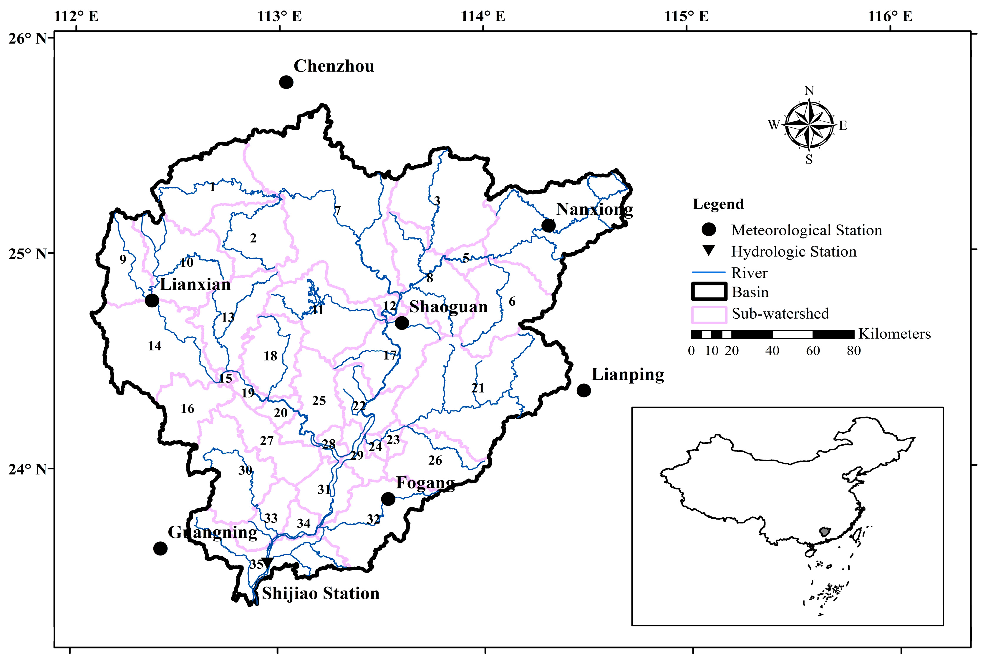
Beijiang River is the second largest tributary of Pearl River Basin and one of the most important water sources in Pearl River Delta, the third largest economic zone in China. Beijiang River Basin, located in the north of Pearl River Basin in southern China (Figure 2), drains a watershed area of 39,220 km2. The basin with complex topography is characterized by mountains and hills, with higher elevations in the north and lower elevations in the south. The region falls within the sub-tropical climate zone, with an average annual temperature of 20 °C and precipitation of 1685 mm, respectively, during the period of 1961–2010. More than 70% of annual precipitation occurs in the wet season (from April to September), while the remainder occurs in the dry season (from December to March). The predominant LUC type in 2010 was forest, followed by cropland, pasture, orchard (e.g., fruit trees and tea trees), construction land and water bodies.
3.2. Dataset
A digital elevation model (DEM) was used, and soil, LUC, meteorological, hydrological and future climate data were collected in this study. The DEM data obtained from the United States Geological Survey (USGS) were used to extract topographic parameters and to delineate the watershed into sub-watersheds. In addition, DEM was used to extract the slopes as a geographical data for LUC prediction. Soil properties were classified based on the Harmonized World Soil Database (HWSD), provided by the Food and Agriculture Organization (FAO). LUC maps from 1990, 2000 and 2010, as well as the other geographical data (roads, railways, cities and towns) used to predict future LUC scenarios were obtained from the Data Center for Resources and Environmental Sciences of Chinese Academy of Sciences. Meteorological data (including daily precipitation and temperature data from 1961 to 2010) were gathered from the Guangdong Meteorological Service. The observed monthly runoff data during 1961–2005 were collected from the Hydrology Bureau of Guangdong Province. Future climate data were obtained from the Norwegian Earth System Model (NorESM) which is a GCM in the Climate Model Intercomparison Project (CMIP5) of the Intergovernmental Panel on Climate Change (IPCC). The daily GCM outputs, which contain precipitation and temperature data for the twentieth and twenty-first centuries from the NorESM, were downloaded from the Lawrence Livermore National Laboratory. The Representative Concentration Pathway (RCP) 4.5 and RCP 8.5 are the two 21st-century scenarios for future greenhouse gas emissions, where RCP 8.5 is a higher emission pathway and RCP 4.5 assumes lower emissions [37].
4. Results and Discussion
4.1. Historical Climate, LUC and Runoff Changes
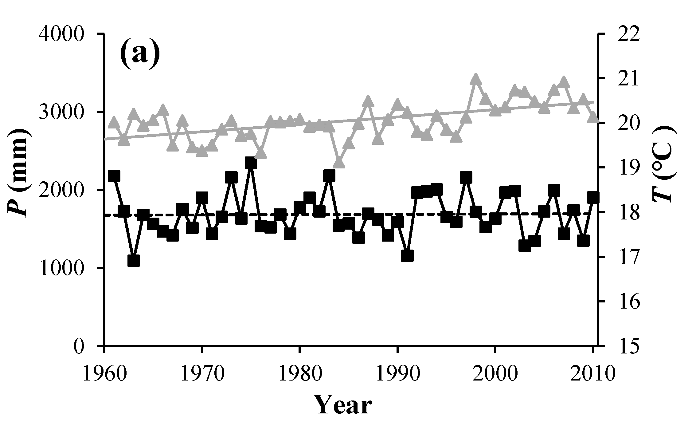
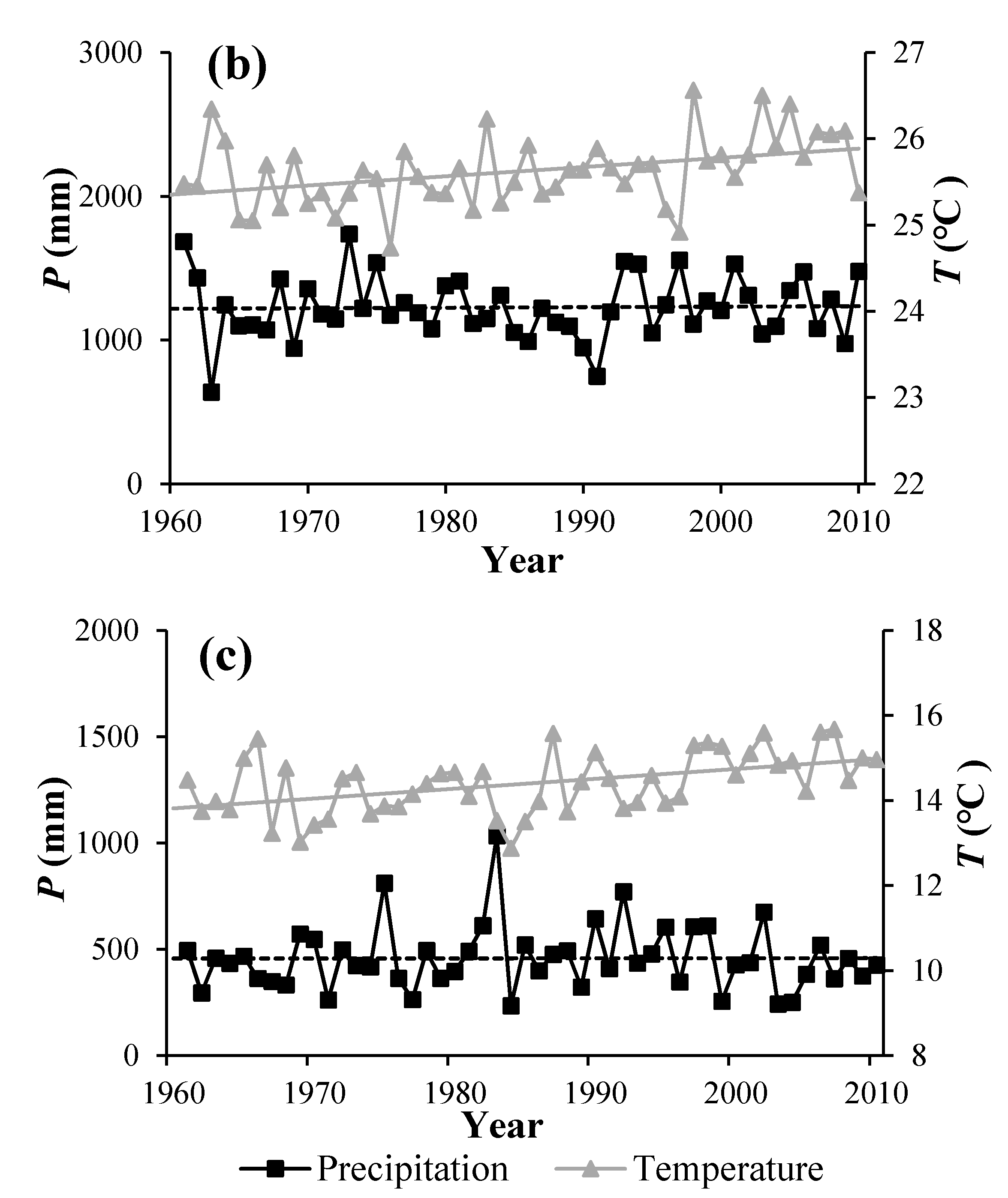
Historical climate change represented by precipitation and temperature from 1961 to 2010 in this case has been analyzed at annual and seasonal (wet and dry) scales. To identify climate change trends, the Mann-Kendall test is adopted and the confidence level is set to 95%. Results of the test show that the average annual precipitation from 1961 to 2010 was 1685 mm with no significant increasing trend (Figure 3). The average precipitation is 1228 mm in the wet season and 457 mm in the dry season. No significant increasing trend in the wet season or decreasing trend in the dry season is detected. The average annual temperature is 20.0 °C, with the presence of a significant increasing trend. The respective temperatures of the wet season and dry season are 25.6 °C and 14.4 °C, with significant increasing trends.
During the period of 1990–2010, Beijiang River Basin experienced considerable changes in its LUC (shown in Figure 4). The orchard area increased by 143% from 1990 to 2010 (Table 1). The area of construction land increased by 40% as a result of population growth and economic development, whereas the areas of pasture, cropland and forest decreased by 5%, 3% and 3%, respectively.
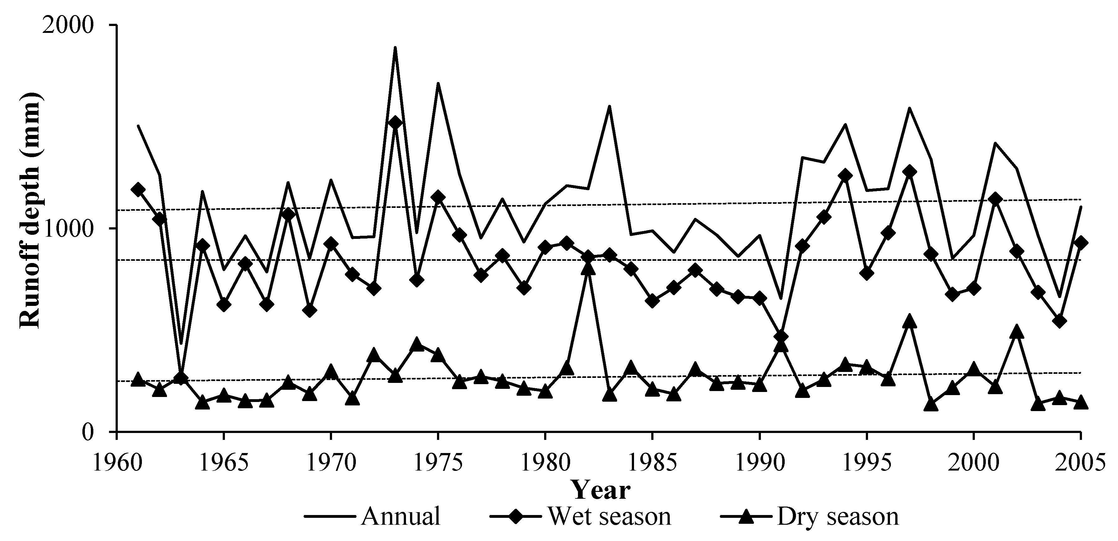
The average annual runoff depth was 1113 mm during 1961–2005, with a nonsignificant upward trend (Figure 5). The runoff depth in the wet season was 843 mm, whereas it was 270 mm in the dry season. The increasing trend in the wet season and the decreasing trend in the dry season were not significant.
4.2. Model Performance
4.2.1. Performance of QM
The performance of QM is assessed by comparing the differences between the statistics (i.e., mean, standard deviation, 95th and 75th percentiles) obtained from the corrections by QM and from observations. The values of these statistics are averaged from seven meteorological stations, and the period from 1961 to 2005 is divided into the calibration period (1961–1990) and the validation period (1991–2005).
The results of the performance assessment of QM are shown in Table 2, where the shaded values (the relative errors larger than 5% of the statistics between the corrections and observations) show a poorer relative performance compared to the unshaded ones. In the calibration period, QM has a good performance with respect to precipitation and temperature, since most of the relative errors of statistics between corrections and observations are less than 5%. However, in the validation period, the performance of QM is not as good as that in the calibration period. Results shows that QM has a poorer performance with respect to precipitation compared with temperature, and QM has a poorer performance in the dry season than in the wet season. The values of relative error during the validation period are found to be the highest for precipitation, and the highest among those (16%) occurs at the 75th percentile in the dry season. This is because the magnitude of precipitation in dry season is much smaller than in wet season, which means that a small bias can cause a large change in the relative error. Additionally, the deviation may be the result of abrupt changes in precipitation in Beijiang River Basin in the 1990s [57] during the validation period. Overall, the performance of QM is generally acceptable, although a certain number of biases still exist after bias correction with QM.
4.2.2. Performance of the CA-Markov Model
Data for LUC in 1990, 2000 and 2010 (LUC1990, LUC2000, LUC2010) in Beijiang River Basin were collected in this study. The observed LUC1990 and LUC2000 were used to facilitate the LUC2010 simulation with the CA-Markov model, and the observed LUC2010 was then compared with the simulated LUC2010 to evaluate the model performance. First, the transition matrix between LUC1990 and LUC2000 was determined using the Markov model. Secondly, the indicators, including elevation, slope, distance to traffic line, distance to the city and distance to the town, were selected to produce transition suitability maps of LUC. Finally, the basis map LUC2000, the transition matrix and the suitability maps were used to simulate LUC2010 with the Markov-CA model. Comparing the observed LUC2010 with the simulated LUC2010 (as shown in Figure 6), the Kappa coefficient is calculated as 0.90, which reveals a high-level agreement between the observed LUC2010 and the simulated one and indicates the CA-Markov model has a strong capacity to simulate LUC. Therefore, with significant effectiveness, the use of the CA-Markov model is acceptable for predicting future LUC in the study area.
4.2.3. Performance of the SWAT Model
After preparing the imported maps (DEM, land use, soil) and database files (e.g., climate, soil properties), the new SWAT project is built for Beijiang River Basin. Model calibration is carried out by adjusting the values of model parameters in the SWAT-CUP (Calibration and Uncertainty Programs for the SWAT model). The SWAT-CUP first identifies the five most sensitive parameters, which are Alpha_BF (baseflow alpha factor), CH_K2 (channel effective hydraulic conductivity), SOL_AWC (water capacity of soil layers), ESCO (soil evaporation compensation factor) and CH_N2 (Manning’s n value for the main channel). Then, model calibration and validation can be carried out.
As the hydrological model parameters may potentially change responding to time-variable precipitation, temperature and LUC [21,58,59,60,61], the time-variant hydrological model is adopted under the changing environment. However, most of the time-variant hydrological models are lumped hydrological models. Even the distributed models that relate spatial changes of LUC to runoff simulation that have been the most commonly used tool to assess the impact of LUC change on runoff, the distributed models with more calibrated parameters are difficult to be transformed into time-variant hydrological model due to limited data. Therefore, the parameters of the SWAT model are calibrated by historical data and are assumed to have extrapolative ability even under the future LUC scenarios in this study. The climate during the historical period (i.e., 1961–2005) and the LUC of early age (i.e., LUC1990) are used for calibration/validation [15,31,32]. The period of 1961–2005 is divided into the calibration period (1961–1990) and the validation period (1991–2005). The values of Ens and R2 during the calibration period are 0.85 and 0.92, and those in the validation are 0.86 and 0.93, respectively. These results show that the peaks and valleys of the simulation similarly correspond to the observations (Figure 7), and the performances of SWAT are satisfactory in the calibration period and the validation period.
4.3. Future Climate and LUC Scenarios
QM is used to correct bias under the RCP 4.5 and RCP 8.5 scenarios. Table 3 shows the percentages of seasonal change in precipitation and temperature between the future period (2011–2050) and the period from 1961 to 2010. Compared to the average annual precipitation in the period of 1961–2010, the one in the period of 2011–2050 increases by 3% under RCP 4.5 and by 8% under RCP 8.5. Precipitation increases by 6% under RCP 4.5 (13% under RCP 8.5) in the wet season and decreases by 1% under RCP 4.5 (3% under RCP 8.5) in the dry season. The average annual temperature in the future period increases by 0.5 °C under RCP 4.5 and by 1.8 °C under RCP 8.5. The temperature increases by 0.7 °C under RCP 4.5 (1.8 °C under RCP 8.5) in the wet season, and increases by 1.5 °C under RCP 4.5 (2.0 °C for RCP 8.5) in the dry season.
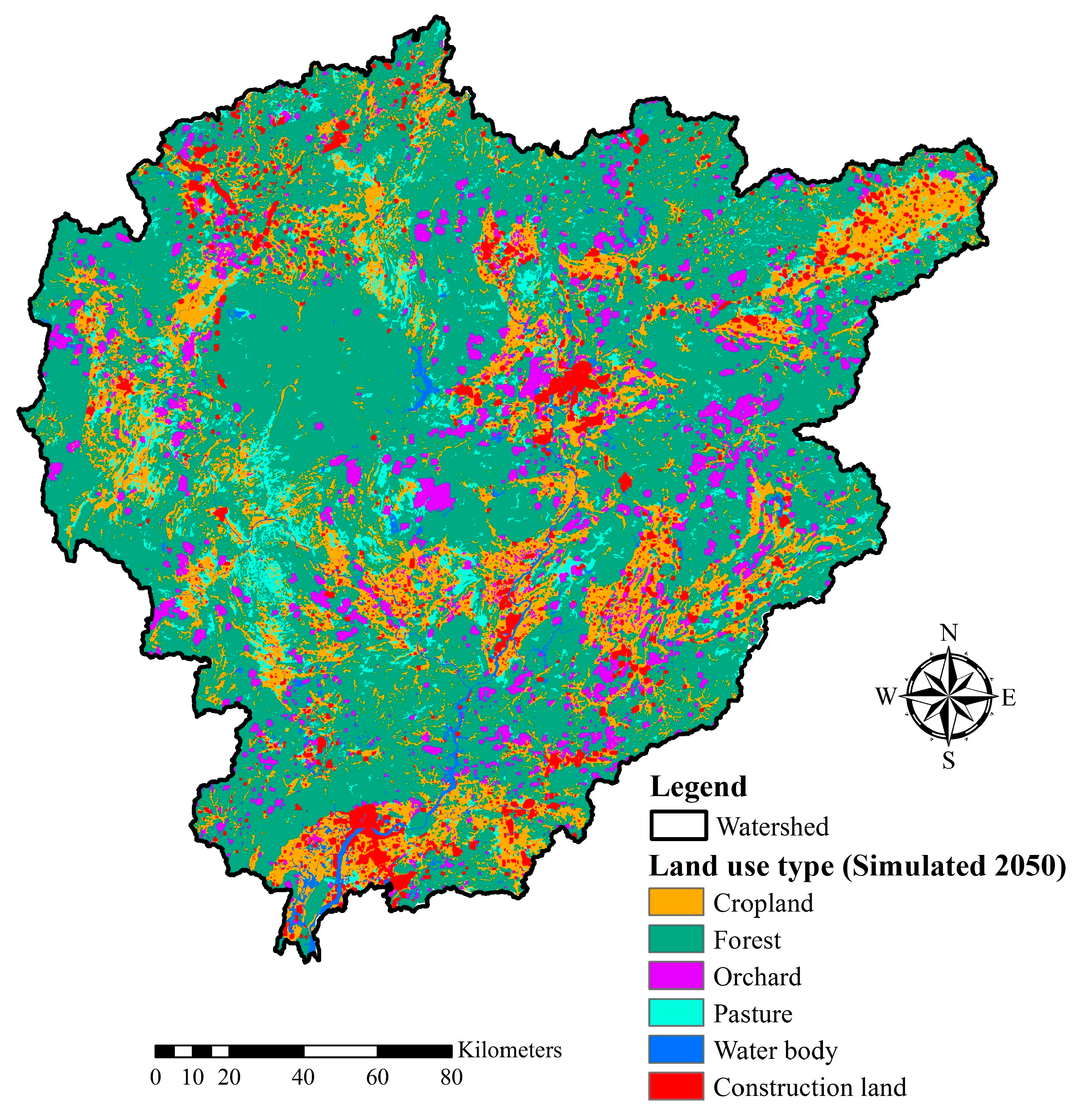
The CA-Markov model is employed to predict future LUC in Beijiang River Basin. Future LUC maps for 2020, 2030, 2040 and 2050 are predicted by the CA-Markov model based on the map LUC2010 (the basis map), the suitability maps and the transition matrix between LUC2000 and LUC2010. From 2010 to 2050, LUC shows the increases in the areas of orchard, construction land and water bodies, but reductions in forest, cropland and pastures (Table 1). In 2050, forest is projected to still be the main LUC type, followed by cropland, orchard, construction land, pasture and water bodies (shown in Figure 8). From 2010 to 2050, the most change occurs in construction land area, with an increase of 132%. The orchard area increases by 128%, whereas the areas of pasture, forest and cropland decrease by 14.3%, 8.6% and 5.7%, respectively.
4.4. Runoff Response to Climate and LUC Changes
To investigate the response of runoff to the projected climate and LUC changes, three types of scenarios (Scenario 1 (LUC of 2010 and climate during the 2011–2050 period, abbreviated S1), Scenario 2 (LUC of 2010, 2020, 2030, 2040 and 2050 and three historical climate conditions, abbreviated S2) and Scenario 3 (LUC of 2010, 2020, 2030, 2040 and 2050 and corresponding climate projections of 2011–2020, 2021–2030, 2031–2040 and 2041–2050 period, abbreviated S3)) are analyzed (Table 4). In S2, in order to reflect the historical climate condition (1961–2010) and simplify the analysis, three typical hydrological years based on the frequency analysis: 1994 (10%), 2000 (50%) and 1985 (90%) are chosen to respectively represent the wet year, normal year and dry year. The impact of climate change on runoff is investigated based on S1, while the impact of LUC change on runoff is studied based on S2. The impact of climate and LUC change simultaneously in the future on runoff is assessed based on S3.
4.4.1. Impact of Climate Change on Runoff Process
S1 is used to assess the impact of climate change on runoff. The results show that the average annual runoff depth in the future period (2011–2050) increases by 9% under RCP 4.5 and by 16% under RCP 8.5 compared to the simulated runoff depth during the period of 1961–2005 (Table 5). Runoff depth increases in both wet and dry seasons under both RCP 4.5 and RCP 8.5. There is an 8% (17%) increase in runoff depth under RCP 4.5 (RCP 8.5) in the wet season, and there is a 10% (12%) increase in runoff depth under RCP 4.5 (RCP 8.5) in the dry season, with a small decline in precipitation and warmer temperatures.
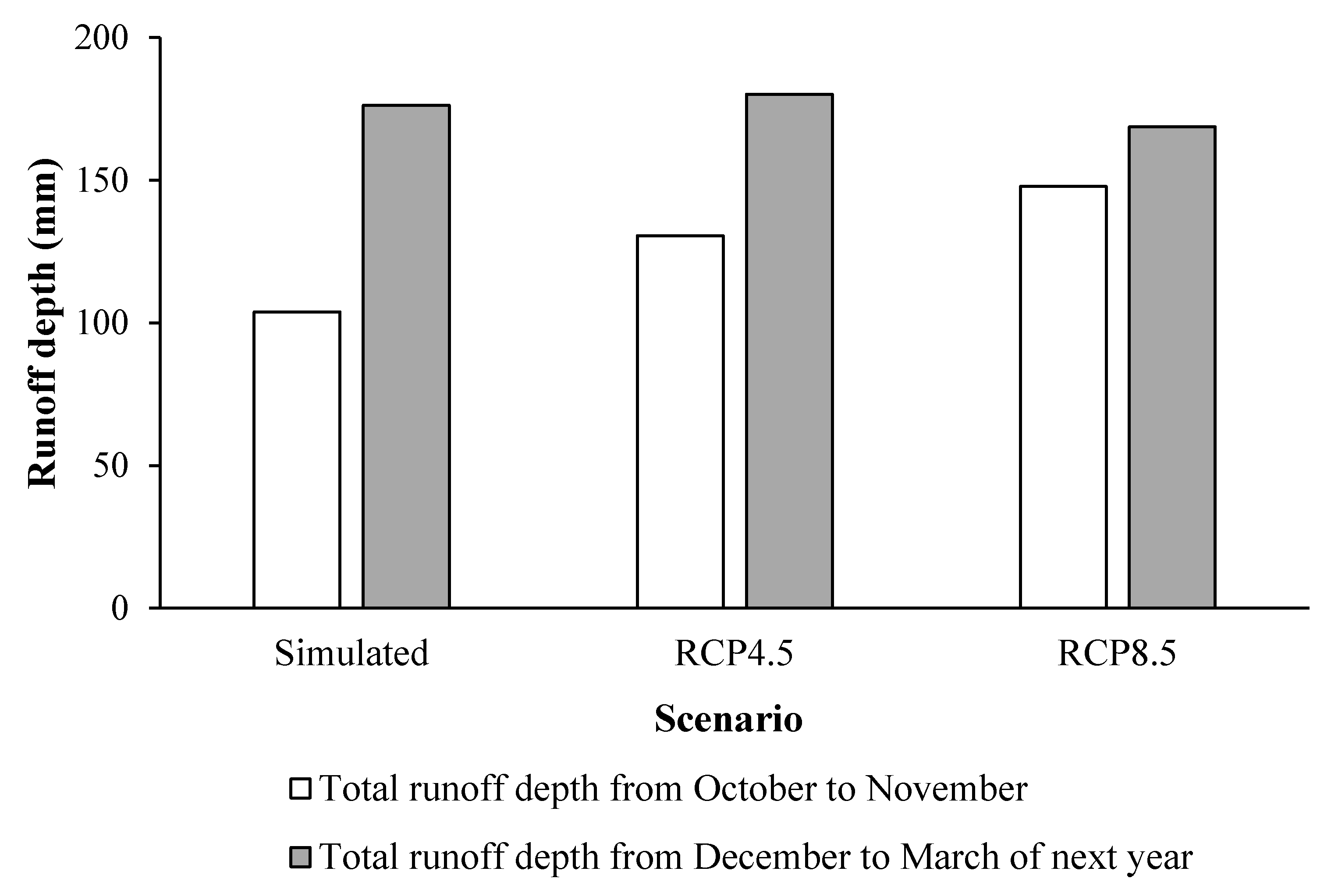
However, increasing runoff depth in the dry season mainly resulted from its increase in the first two months of the season (October and November). The mean value of simulated runoff depth during 1961–2005 is 103 mm from October to November. The simulated runoff depth is 176 mm in the other four months during the dry season (from December to March of the next year). It is clear that the increase in predicted runoff depth in the whole dry season is mostly caused by the increased runoff depth in October and November under RCP 4.5 and RCP 8.5 (Figure 9). The mean values of predicted runoff depth from October to November during 2011–2050 are 130 mm under RCP 4.5 and 148 mm under RCP 8.5, whereas the predicted runoff depths are 180 mm under RCP 4.5 and 168 mm under RCP 8.5 from December to March in the following year. The greater increase in runoff depth in the wet season results in the greater runoff depth in the first two months in the dry season (27 mm under RCP 4.5 and 45 mm under RCP 8.5), because those months are more strongly influenced by the recession flow of the wet season. In the last four months of the dry season, little variation is present between the predicted runoff depth under RCP 4.5 and the simulated runoff depth. However, under RCP 8.5, the predicted runoff depth is lower than the simulated runoff depth because of a slight reduction in precipitation and warmer temperatures from December to March in the following year.
4.4.2. Impact of LUC Change on Runoff Process
The response of runoff to LUC change is investigated with different LUC scenarios (LUC2010, LUC2020, LUC2030, LUC2040 and LUC2050) and three typical hydrological years (S2 as shown in Table 4). Results show a few differences in runoff at the outlet of the whole basin under the LUC2010, LUC2020, LUC2030, LUC2040 and LUC2050 scenarios for the wet, normal and dry years (shown in Figure 10). It can therefore be concluded that LUC change has little influence on the variation in runoff at the whole-basin level.
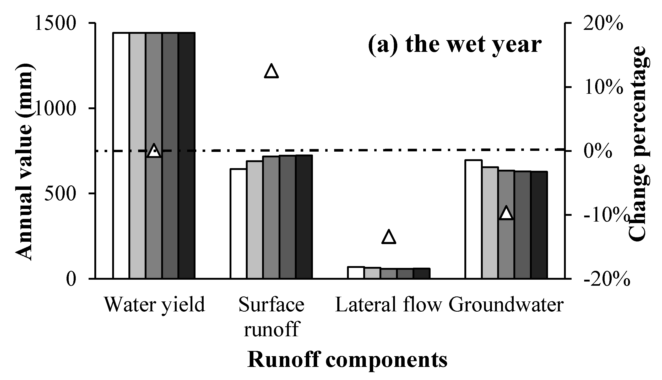
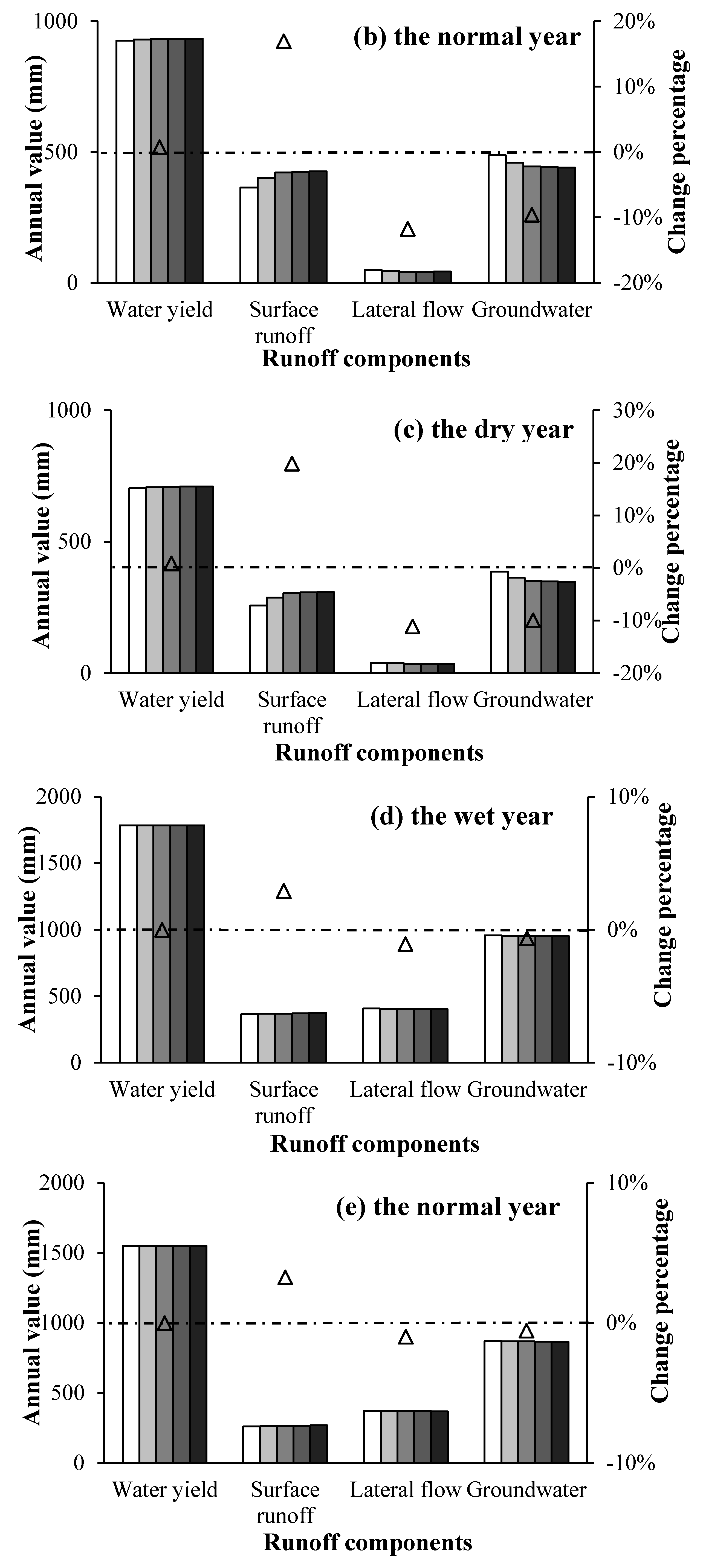
The impacts of spatial distribution of LUC on runoff at the sub-watershed level are assessed by analyzing the runoff components in the different hydrological years. According to the spatial analysis module in the SWAT model, the whole Beijiang River Basin is divided into 35 sub-watersheds (shown in Figure 2), where the two typical sub-watersheds with different special distributions of LUC (Sub12 and Sub31) are selected. Sub12 represents an urbanized area which is expected to undergo further drastic urbanization, from 22.5% in 2010 to 40.7% in 2050 (shown in Table 6). Sub31 is selected as a region where the natural conditions are maintained, with only 7% conversion from forest to orchard. Figure 11 shows the impact of LUC change on the runoff components of Sub12 and Sub31 in different hydrological years. In Sub12, the water yield and surface runoff increase due to rapid urbanization, whereas lateral flow and groundwater decrease. The LUC change from 2010 to 2050 has little impact on the annual water yield. There is almost no change in water yield for the wet year, but a slight increase occurs in the normal and dry years, as shown in Figure 11a–c. Surface runoff and groundwater are found to be more sensitive to LUC change than the lateral flow. The LUC change from 2010 to 2050 increases the surface runoff in the wet year by 81 mm (13%); in the normal year by 62 mm (17%), and in the dry year by 51 mm (19%). Urbanization decreases groundwater in the wet year by 67 mm (10%), in the normal year by 47 mm (10%), and in the dry year by 38 mm (10%). The changes in surface runoff and groundwater may be attributed to the expansion of impermeable land surface, which makes rainwater flow directly into the river and decreases soil infiltration. The increase of surface runoff and the decline of lateral flow and groundwater are much higher in the wet year than in the normal and dry years. Zhou et al. [56] reached similar results. However, the results concerning Sub31 with natural conditions show no change in annual water yield, surface runoff, lateral flow or groundwater, as shown in Figure 11d–f. For each different hydrological year, few significant differences in runoff components influenced by LUC change are detected in Sub31. Therefore, important significant changes will occur in the allocation between surface runoff and groundwater in urbanized region, but insignificant changes in runoff generation processes are anticipated under natural conditions.
4.4.3. Impact of Climate and LUC Changes on Runoff Process
Runoff prediction under S3 is proposed to represent the runoff response to climate and LUC change simultaneously during the future period of 2011–2050 (shown in Figure 12). The average annual runoff depth in the future period increases by 9% under RCP 4.5 and by 16% under RCP 8.5, compared to the simulated runoff depth during the historical period of 1961–2005. Runoff depths in the wet season rise by 8% under the RCP 4.5 scenario and by 16% under the RCP 8.5 scenario, whereas the runoff depth in the dry season increases by 14% under RCP 4.5 and by 16% under RCP 8.5. Overall, considering the whole basin, climate change plays a dominant role in altering runoff process, whereas LUC change has little influence on change in runoff.
The runoff process is influenced by both climate change and LUC change with intensive anthropogenic activities, especially in urbanized regions. In Sub12, a comparison between the results from S1 and S3 shows that the water yield and surface runoff increase under both RCP 4.5 and RCP 8.5 scenarios (shown in Figure 13). However, LUC change decreases lateral flow and groundwater during the period from 2011 to 2050. Surface runoff increases by 51 mm (11%), and groundwater decreases by 39 mm (8%) in S3 under RCP 4.5, whereas there is a 50 mm (10%) increase of surface runoff and a 38 mm (8%) decrease of groundwater under RCP 8.5. Changes in surface runoff and groundwater are therefore sensitive to LUC change in urbanized regions. Moreover, water yield and lateral flow slightly increase and decrease, respectively. Therefore, urbanization can influence the allocation between surface runoff and groundwater, as discussed in Section 4.4.2.
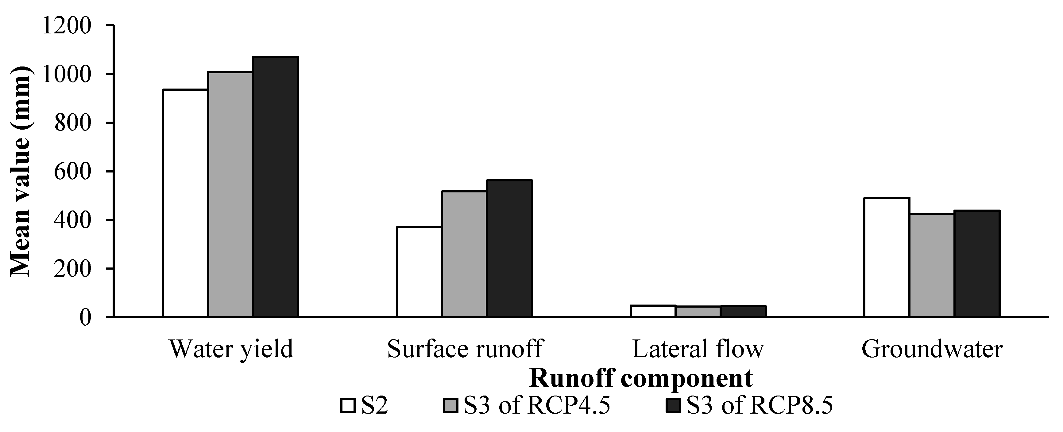
By comparing the results from S2 and S3, climate change will increase water yield and surface runoff, whereas it will decrease the groundwater component and have an insignificant influence on lateral flow, based on LUC2010 under S2 (Figure 14). In S3, the water yield increases by 73 mm (8%) under RCP 4.5 and by 135 mm (14%) under RCP 8.5, and surface runoff increases by 147 mm (40%) under RCP 4.5 and by 192 mm (51%) under RCP 8.5. Changes in runoff components and allocation between surface runoff and groundwater are therefore found to be more severe under RCP 8.5 than under RCP 4.5 in scenario S3.
5. Conclusions
The aim of this study is to examine future runoff response to climate and LUC changes in Beijiang River Basin in China. The climate scenarios are projected by downscaling GCM outputs using the QM method, and the future LUC scenarios are predicted with the CA-Markov model. The SWAT model is adopted to assess runoff responses of the study area by investigating and comparing the results of S1, S2 and S3. The following conclusions can be drawn:
- (1)
- The impact of climate change on runoff is significant. Runoff depth is projected to increase in both wet and dry seasons under future climate change for both RCP 4.5 and RCP 8.5.
- (2)
- LUC change has an insignificant influence on runoff at the basin level, since there are few differences in outlet runoff under different LUC scenarios. However, changes in runoff components are more important at the sub-watershed level. The impact of urbanization on runoff components can be better understood at the sub-watershed level, and urbanization has less impact on water yield than on surface runoff and groundwater. The impact of LUC change on runoff components differs obviously among the wet, normal and dry years in urbanized regions. The increase in surface runoff caused by urbanization is highest in the wet year.
- (3)
- With simultaneous changes in climate and LUC, runoff depth in the study area is predicted to increase in the future. Climate change brings increases in water yield and surface runoff, whereas LUC change leads to changes in the allocation of surface runoff and groundwater in urban areas.
In this research, the future climate scenarios are projected based on a GCM, and the future LUC scenarios are predicted based on a LUC simulated model. However, the changes in climate and LUC in the future period are uncertain not only for the scenarios but also for the calibrated parameter of the hydrological model. Therefore, in the future research, it is suggested to collect more GCMs and use different LUC simulated models to predict the future climate scenarios and LUC scenarios, respectively. It is also recommended to investigate the uncertainties of the two types of scenarios and the stationarity of the calibrated parameters of the models, as well as the future runoff response to the different combinations of climate and LUC scenarios.
Acknowledgments
The authors gratefully acknowledge financial support from the National Natural Science Foundation of China (No. 51379148, 51579183, 91647106 and 51525902) and the Science and Technology Program of Guangzhou City (No. 201707010072). Great thanks to Xi Xuan Yu from McGill University (Canada) to polish this manuscript.
Author Contributions
D.L., P.L. and L.X. proposed the methodology of this study; Z.W., Q.Z. and H.Z. collected the data; Y.H. and S.P. analyzed the data; S.P. wrote the paper; D.L., P.L. and L.X. revised the paper.
Conflicts of Interest
The authors declare no conflict of interest.
References
- Changnon, S.A.; Demissie, M. Detection of changes in streamflow and floods resulting from climate fluctuations and land use-drainage changes. Clim. Chang. 1996, 32, 411–421. [Google Scholar] [CrossRef]
- Jung, M.; Reichstein, M.; Ciais, P.; Seneviratne, S.I.; Sheffield, J.; Goulden, M.L.; Bonan, G.; Cescatti, A.; Chen, J.; Jeu, R.D.; et al. Recent decline in the global land evapotranspiration trend due to limited moisture supply. Nature 2010, 467, 951–954. [Google Scholar] [CrossRef] [PubMed]
- Costa, M.H.; Botta, A.; Cardille, J.A. Effects of large-scale changes in land cover on the discharge of the Tocantins River, Southeastern Amazonia. J. Hydrol. 2003, 283, 206–217. [Google Scholar] [CrossRef]
- Jones, J.A. Hydrologic processes and peak discharge response to forest removal, regrowth, and roads in 10 small experimental basins, western Cascades, Oregon. Water Resour. Res. 2000, 36, 2621–2642. [Google Scholar] [CrossRef]
- Mishra, S.K.; Singh, V.P. Soil conservation service curve number (SCS-CN) methodology. Water Sci. Technol. Libr. 2003, 22, 355–362. [Google Scholar]
- Tao, F.L.; Yokozawa, M.; Hayashi, Y.; Lin, E. Future climate change, the agricultural water cycle, and agricultural production in China. Agric. Ecosyst. Environ. 2003, 95, 203–215. [Google Scholar] [CrossRef]
- Yan, L.; Xiong, L.H.; Liu, D.D.; Hu, T.S.; Xu, C.Y. Frequency analysis of nonstationary annual maximum flood series using the time-varying two-component mixture distributions. Hydrol. Process. 2017, 31, 69–89. [Google Scholar] [CrossRef]
- Vörösmarty, C.J.; Green, P.; Salisbury, J.; Lammers, R.B. Global water resources: Vulnerability from climate change and population growth. Science 2000, 289, 284–288. [Google Scholar] [CrossRef] [PubMed]
- Ma, X.; Xu, J.C.; Noordwijk, M.V. Sensitivity of streamflow from a Himalayan catchment to plausible changes in land cover and climate. Hydrol. Process. 2010, 24, 1379–1390. [Google Scholar] [CrossRef]
- Chawla, I.; Mujumdar, P.P. Isolating the impacts of land use and climate change on streamflow. Hydrol. Earth Syst. Sci. 2015, 19, 3633–3651. [Google Scholar] [CrossRef]
- Tranga, N.T.T.; Shresthaa, S.; Shresthaa, M.; Dattab, A.; Kawasakic, A. Evaluating the impacts of climate and land-use change on the hydrology and nutrient yield in a transboundary river basin: A case study in the 3S River Basin (Sekong, Sesan, and Srepok). Sci. Total Environ. 2017, 576, 586–598. [Google Scholar] [CrossRef] [PubMed]
- Wang, S.F.; Kang, S.Z.; Zhang, L.; Li, F.S. Modelling hydrological response to different land-use and climate change scenarios in the Zamu River basin of northwest China. Hydrol. Process. 2008, 22, 2502–2510. [Google Scholar] [CrossRef]
- Goyal, M.K.; Burn, D.H.; Ojha, C.S.P. Statistical downscaling of temperatures under climate change scenarios for Thames river basin, Canada. Int. J. Glob. Warm. 2012, 4, 13–30. [Google Scholar] [CrossRef]
- Li, F.P.; Zhang, Y.Q.; Xu, Z.X.; Teng, J.; Liu, C.M.; Liu, W.F.; Mpelasoka, F. The impact of climate change on runoff in the southeastern Tibetan Plateau. J. Hydrol. 2013, 505, 188–201. [Google Scholar] [CrossRef]
- Gan, R.; Luo, Y.; Zuo, Q.T.; Sun, L. Effects of projected climate change on the glacier and runoff generation in the Naryn River Basin, Central Asia. J. Hydrol. 2015, 523, 240–251. [Google Scholar] [CrossRef]
- Dhar, S.; Mazumdar, A. Hydrological modelling of the Kangsabati river under changed climate scenario: Case study in India. Hydrol. Process. 2009, 23, 2394–2406. [Google Scholar] [CrossRef]
- Chen, H.; Xu, C.Y.; Guo, S.L. Comparison and evaluation of multiple GCMs, statistical downscaling and hydrological models in the study of climate change impacts on runoff. J. Hydrol. 2012, 434–435, 36–45. [Google Scholar] [CrossRef]
- Bosch, J.M.; Hewlett, J.D. A review of catchment experiments to determine the effect of vegetation changes on water yield and evapotranspiration. J. Hydrol. 1982, 55, 3–23. [Google Scholar] [CrossRef]
- Hornbeck, J.W.; Adams, M.B.; Corbett, E.S.; Verry, E.S.; Lynch, J.A. Long-term impacts of forest treatments on water yield: A summary for northeastern USA. J. Hydrol. 1993, 150, 323–344. [Google Scholar] [CrossRef]
- Stednick, J.D. Monitoring the effects of timber harvest on annual water yield. J. Hydrol. 1996, 176, 79–95. [Google Scholar] [CrossRef]
- Brown, A.E.; Zhang, L.; McMahon, T.A.; Western, A.W.; Vertessy, R.A. A review of paired catchment studies for determining changes in water yield resulting from alterations in vegetation. J. Hydrol. 2005, 310, 28–61. [Google Scholar] [CrossRef]
- Onstad, C.A.; Jamieson, D.G. Modelling the effect of land use modifications on runoff. Water Resour. Res. 1970, 6, 1287–1295. [Google Scholar] [CrossRef]
- Calder, I.R.; Hall, R.L.; Bastable, H.G.; Gunston, H.M.; Shela, O.; Chirwa, A.; Kafundu, R. The impact of land use change on water resources in sub-Saharan Africa: A modelling study of Lake Malawi. J. Hydrol. 1995, 170, 123–135. [Google Scholar] [CrossRef]
- Fohrer, N.; Haverkamp, S.; Frede, H.G. Assessment of the effects of land use patterns on hydrologic landscape functions: Development of sustainable land use concepts for low mountain range areas. Hydrol. Process. 2005, 19, 659–672. [Google Scholar] [CrossRef]
- Li, L.J.; Jiang, D.J.; Hou, X.Y.; Li, J.Y. Simulated runoff responses to land use in the middle and upstream reaches of Taoerhe River basin, Northeast China, in wet, average and dry years. Hydrol. Process. 2013, 27, 3484–3494. [Google Scholar] [CrossRef]
- Mwangi, H.M.; Julich, S.; Patil, S.D.; McDonald, M.A.; Feger, K.H. Modelling the impact of agroforestry on hydrology of MaraRiver Basin in East Africa. Hydrol. Process. 2016, 30, 3139–3155. [Google Scholar] [CrossRef]
- Li, F.P.; Zhang, G.X.; Xu, Y.J. separating the impacts of climate variation and human activities on runoff in the songhua river basin, northeast China. Water 2014, 6, 3320–3338. [Google Scholar] [CrossRef]
- Zhan, C.S.; Jiang, S.S.; Sun, F.B.; Jia, Y.W.; Niu, C.W.; Yue, W.F. Quantitative contribution of climate change and human activities to runoff changes in the Wei River basin, China. Hydrol. Earth Syst. Sci. 2014, 18, 3069–3077. [Google Scholar] [CrossRef]
- Zhang, X.P.; Zhang, L.; Zhao, J.; Rustomji, P; Hairsine, P. Responses of streamflow to changes in climate and land use/cover in the Loess Plateau, China. Water Resour. Res. 2008, 44, W00A07. [Google Scholar] [CrossRef]
- Li, Z.; Liu, W.Z.; Zhang, X.C.; Zheng, F.L. Impacts of land use change and climate variability on hydrology in an agricultural catchment on the Loess Plateau of China. J. Hydrol. 2009, 377, 35–42. [Google Scholar] [CrossRef]
- Cuo, L.; Zhang, Y.X.; Gao, Y.H.; Hao, Z.C.; Cairang, L. The impacts of climate change and land cover/use transition on the hydrology in the upper Yellow River Basin, China. J. Hydrol. 2013, 502, 37–52. [Google Scholar] [CrossRef]
- Zhang, L.; Karthikeyan, R.; Bai, Z.K.; Srinivasan, R. Analysis of streamflow responses to climate variability and land use change in the Loess Plateau region of China. Catena 2017, 154, 1–11. [Google Scholar] [CrossRef]
- Chen, J.; Brissette, F.P.; Chaumont, D.; Braun, M. Performance and uncertainty evaluation of empirical downscaling methods in quantifying the climate change impacts on hydrology over two North American river basins. J. Hydrol. 2013, 479, 200–214. [Google Scholar] [CrossRef]
- Mouria, G.; Nakanob, K.; Tsuyamac, I.; Tanakac, N. The effects of future nationwide forest transition to discharge in the 21st century with regard to general circulation model climate change scenarios. Environ. Res. 2016, 149, 288–296. [Google Scholar] [CrossRef] [PubMed]
- Themeßl, M.J.; Gobiet, A.; Leuprecht, A. Empirical-statistical downscaling and error correction of daily precipitation from regional climate models. Int. J. Climatol. 2011, 31, 1530–1544. [Google Scholar] [CrossRef]
- Themeßl, M.J.; Gobiet, A.; Heinrich, G. Empirical-statistical downscaling and error correction of regional climate models and its impact on the climate change signal. Clim. Chang. 2012, 112, 449–468. [Google Scholar] [CrossRef]
- Wang, L.; Chen, W. A CMIP5 multimodel projection of future temperature, precipitation, and climatological drought in China. Int. J. Climatol. 2014, 34, 2059–2078. [Google Scholar] [CrossRef]
- Ngai, S.T.; Tangang, F.; Juneng, L. Bias correction of global and regional simulated daily precipitation and surface mean temperature over Southeast Asia using quantile mapping method. Glob. Planet. Chang. 2017, 149, 79–90. [Google Scholar] [CrossRef]
- Maraun, D. Bias correction, quantile mapping, and downscaling: Revisiting the inflation issue. J. Clim. 2013, 26, 2137–2143. [Google Scholar] [CrossRef]
- Teutschbein, C.; Seibert, J. Bias correction of regional climate model simulations for hydrological climate-change impact studies: Review and evaluation of different methods. J. Hydrol. 2012, 456–457, 12–29. [Google Scholar] [CrossRef]
- Mpelasoka, F.S.; Chiew, F.H.S. Influence of rainfall scenario construction methods on runoff projections. J. Hydrometeorol. 2009, 10, 1168–1183. [Google Scholar] [CrossRef]
- Hyandye, C.; Martz, L.W. A Markovian and cellular automata land-use change predictive model of the Usangu Catchment. Int. J. Remote Sens. 2017, 38, 64–81. [Google Scholar] [CrossRef]
- Nouri, J.; Gharagozlou, A.; Arjmandi, R.; Faryadi, S.; Adl, M. Predicting urban land use changes using a CA-Markova model. Arab. J. Sci. Eng. 2014, 39, 5565–5573. [Google Scholar] [CrossRef]
- Halmy, M.W.A.; Gessler, P.E.; Hicke, J.A.; Salem, B.B. Land use/land cover change detection and prediction in the north-western coastal desert of Egypt using Markov-CA. Appl. Geogr. 2015, 63, 101–112. [Google Scholar] [CrossRef]
- Memarian, H.; Balasundram, S.K.; Talib, J.B.; Sung, C.T.B.; Sood, A.M.; Abbaspour, K. Validation of CA-Markov for simulation of land use and cover change in the langat basin, Malaysia. J. Geogr. Inf. Syst. 2012, 4, 542–554. [Google Scholar] [CrossRef]
- Guan, D.J.; Li, H.F.; Inohae, T.; Su, W.C.; Nagaie, T.; Hokao, K. Modeling urban land use change by the integration of cellular automaton and Markov model. Ecol. Model. 2011, 222, 3761–3772. [Google Scholar] [CrossRef]
- Scott, W.A. The reliability of content analysis: The case of nominal scale coding. Pub. Opin. Q. 1955, 19, 321–325. [Google Scholar] [CrossRef]
- Arnold, J.G.; Srinivasan, R.; Muttiah, R.S.; Williams, J.R. Large area hydrologic modeling and assessment. Part 1. Model development. J. Am. Water Resour. Assoc. 1998, 34, 1–17. [Google Scholar] [CrossRef]
- Mango, L.M.; Melesse, A.M.; McClain, M.E.; Gann, D.; Setegn, S.G. Land use and climate change impacts on the hydrology of the upper Mara River Basin, Kenya: Results of a modeling study to support better resource management. Hydrol. Earth Syst. Sci. 2011, 15, 2245–2258. [Google Scholar] [CrossRef]
- Wagner, P.D.; Kumar, S.; Schneider, K. An assessment of land use change impacts on the water resources of the Mula and Mutha Rivers catchment upstream of Pune, India. Hydrol. Earth Syst. Sci. 2013, 17, 2233–2246. [Google Scholar] [CrossRef]
- Mehdi, B.; Ludwig, R.; Lehner, B. Evaluating the impacts of climate change and crop land use change on streamflow, nitrates and phosphorus: A modeling study in Bavaria. J. Hydrol. Reg. Stud. 2015, 4, 60–90. [Google Scholar] [CrossRef]
- Zhang, L.; Nan, Z.T.; Yu, W.J.; Ge, Y.C. Hydrological responses to land-use change scenarios under constant and changed climatic conditions. Environ. Manag. 2016, 57, 412–431. [Google Scholar] [CrossRef] [PubMed]
- Eckhardt, K.; Ulbrich, U. Potential impacts of climate change on groundwater recharge and streamflow in a central European low mountain range. J. Hydrol. 2003, 284, 244–252. [Google Scholar] [CrossRef]
- Bouraoui, F.; Grizzetti, B.; Granlund, K.; Rekolainen, S.; Bidoglio, G. Impact of climate change on the water cycle and nutrient losses in a Finnish catchment. Clim. Chang. 2004, 66, 109–126. [Google Scholar] [CrossRef]
- Neitsch, S.L.; Arnold, J.R.; Williams, J.R. Soil and Water Assessment Tool Theoretical Documentation, Version 2009. Available online: http://swat.tamu.edu/documentation/ (accessed on 28 June 2017).
- Zhou, F.; Xu, Y.P.; Chen, Y.; Xu, C.Y.; Gao, Y.Q.; Du, J.K. Hydrological response to urbanization at different spatio-temporal scales simulated by coupling of CLUE-S and the SWAT model in the Yangtze River Delta region. J. Hydrol. 2013, 485, 113–125. [Google Scholar] [CrossRef]
- Li, Y.; Chen, X.H.; Wang, Z.L. A tentative discussion on the impact of human activities on the variability of runoff series of the Beijiang River basin. J. Nat. Resour. 2006, 21, 910–915. (In Chinese) [Google Scholar]
- Andréassian, V.; Parent, E.; Michel, C. A distribution-free test to detect gradual changes in 358 watershed behavior. Water Resour. Res. 2003, 39, 333–342. [Google Scholar] [CrossRef]
- Merz, R.; Parajka, J.; Blöschl, G. Time stability of catchment model parameters: Implications for climate impact analyses. Water Resour. Res. 2011, 47, 2144–2150. [Google Scholar] [CrossRef]
- Westra, S.; Thyer, M.; Leonard, M.; Kavetski, D.; Lambert, M. A strategy for diagnosing and interpreting hydrological model nonstationarity. Water Resour. Res. 2014, 50, 5090–5113. [Google Scholar] [CrossRef]
- Patil, S.D.; Stieglitz, M. Comparing spatial and temporal transferability of hydrological model parameters. J. Hydrol. 2015, 525, 409–417. [Google Scholar] [CrossRef]
Figure 1.
Overview of the proposed methodology.
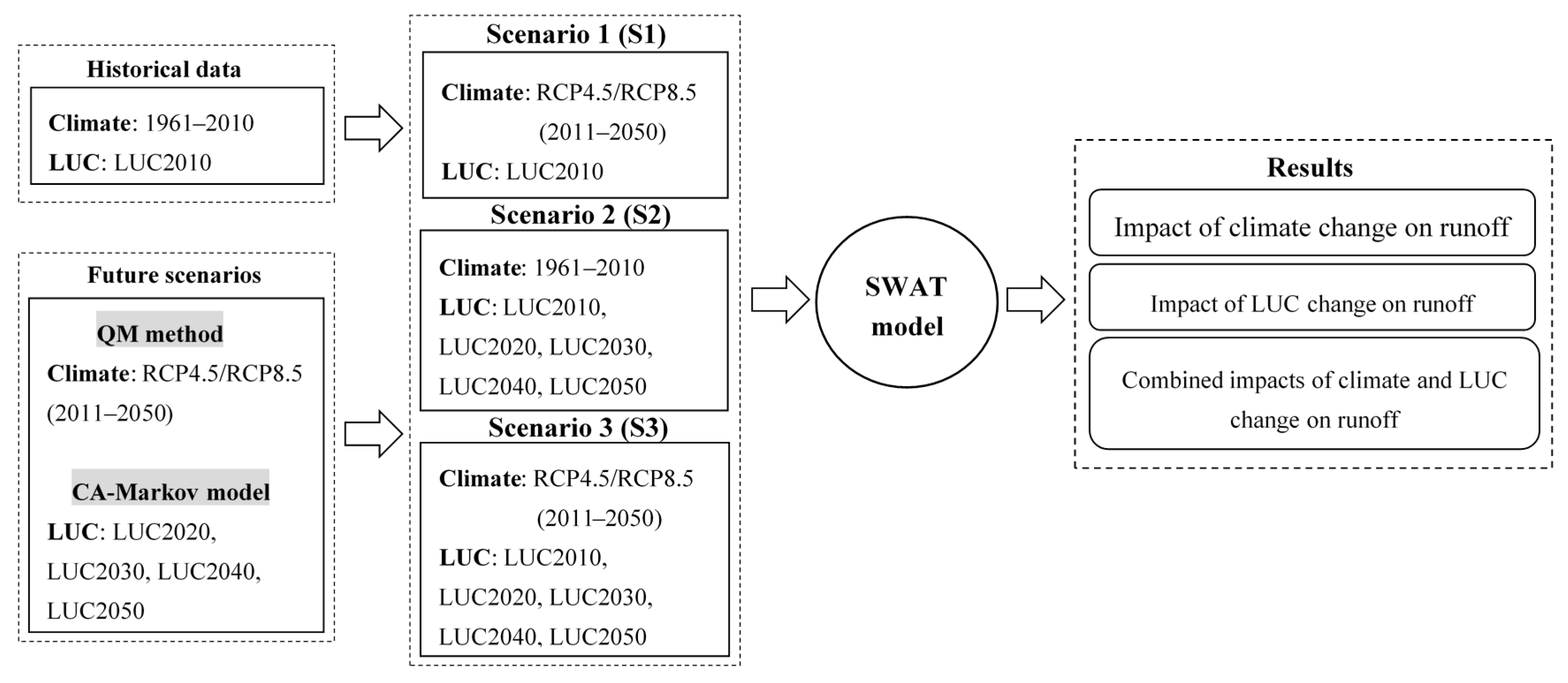
Figure 2.
Location and sub-watersheds delineation of the Beijiang River basin in China.

Figure 3.
Variations in average precipitation (P) and temperature (T) at annual (a) and seasonal (wet season (b) and dry season (c)) scales from 1961–2010. The solid linear line represents the significant increasing/decreasing trend at a 95% level, and the dashed line shows a nonsignificant trend.
Figure 3.
Variations in average precipitation (P) and temperature (T) at annual (a) and seasonal (wet season (b) and dry season (c)) scales from 1961–2010. The solid linear line represents the significant increasing/decreasing trend at a 95% level, and the dashed line shows a nonsignificant trend.


Figure 4.
LUC of Beijiang River Basin in 2010.
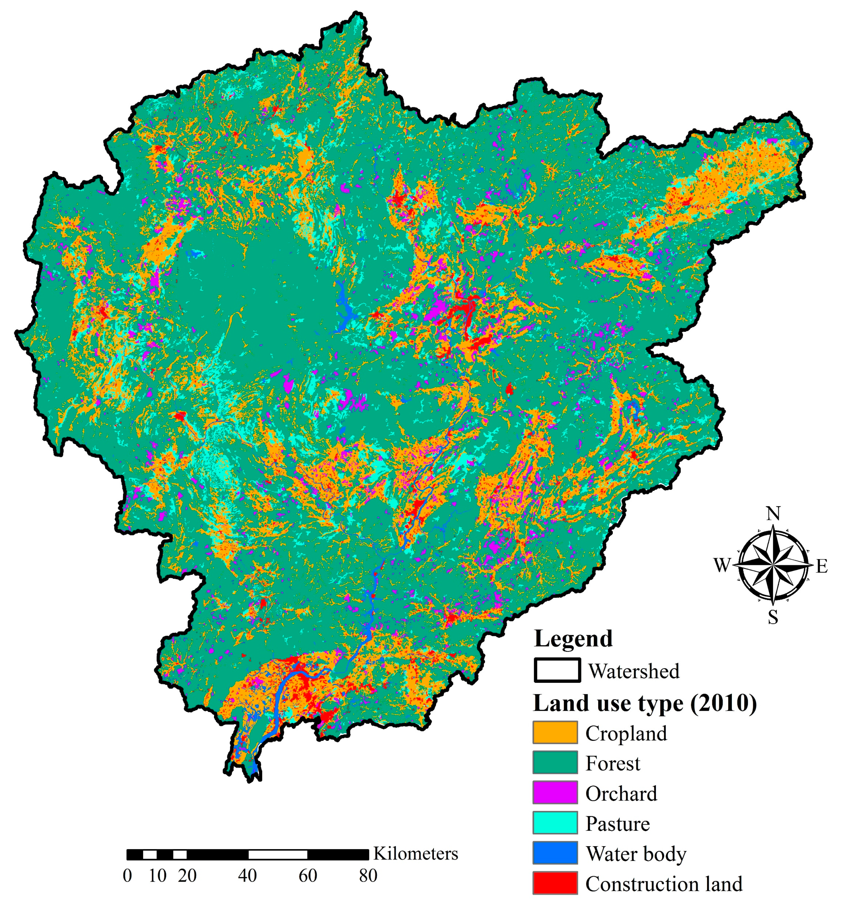
Figure 5.
Variation in runoff depth from 1961 to 2005. The dashed line shows a nonsignificant trend.
Figure 5.
Variation in runoff depth from 1961 to 2005. The dashed line shows a nonsignificant trend.

Figure 6.
Simulated LUC of Beijiang River Basin in 2010.
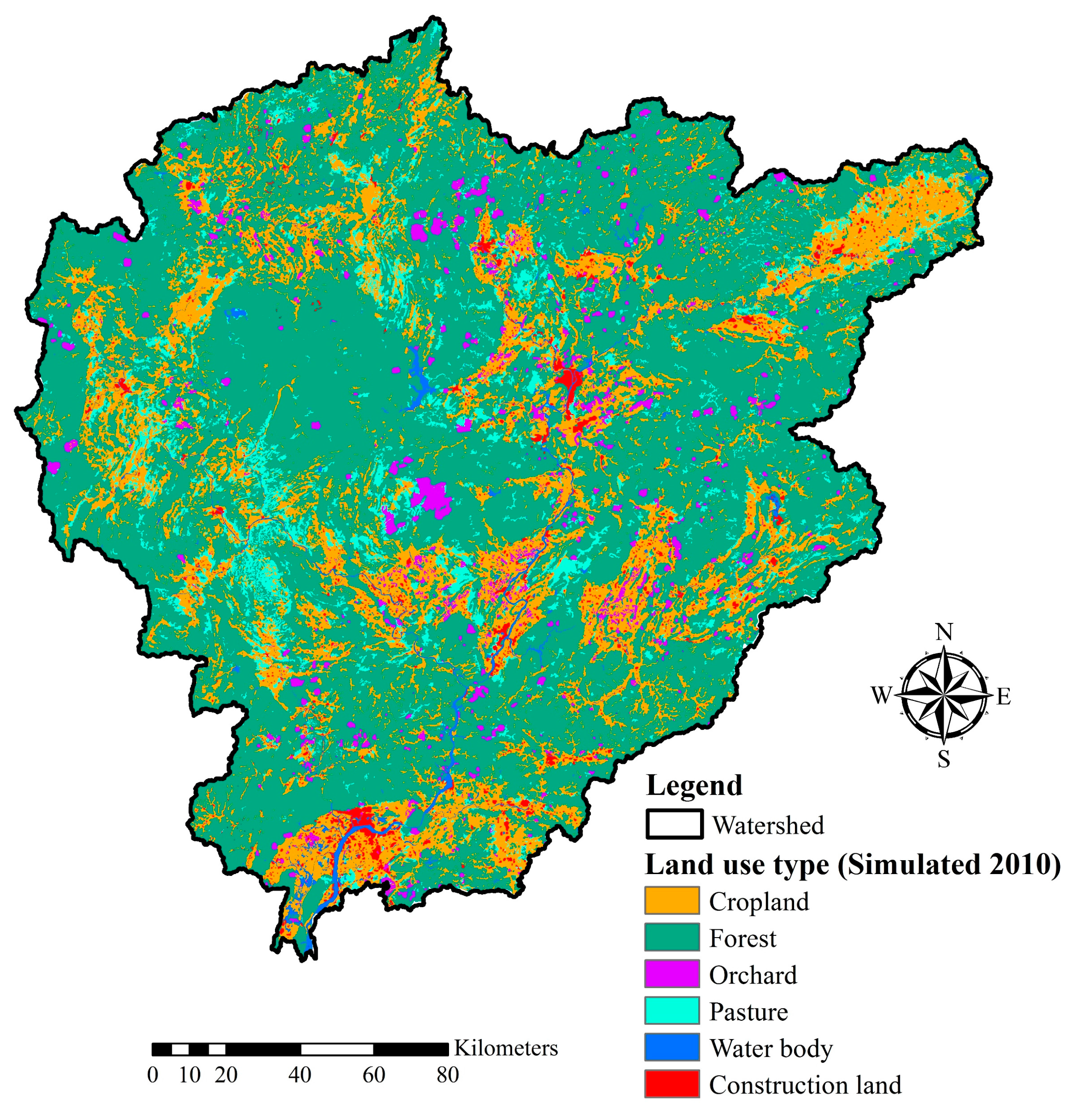
Figure 7.
Comparison of simulated and observed monthly runoff in the calibration period (1961–1990) and validation period (1991–2005).
Figure 7.
Comparison of simulated and observed monthly runoff in the calibration period (1961–1990) and validation period (1991–2005).
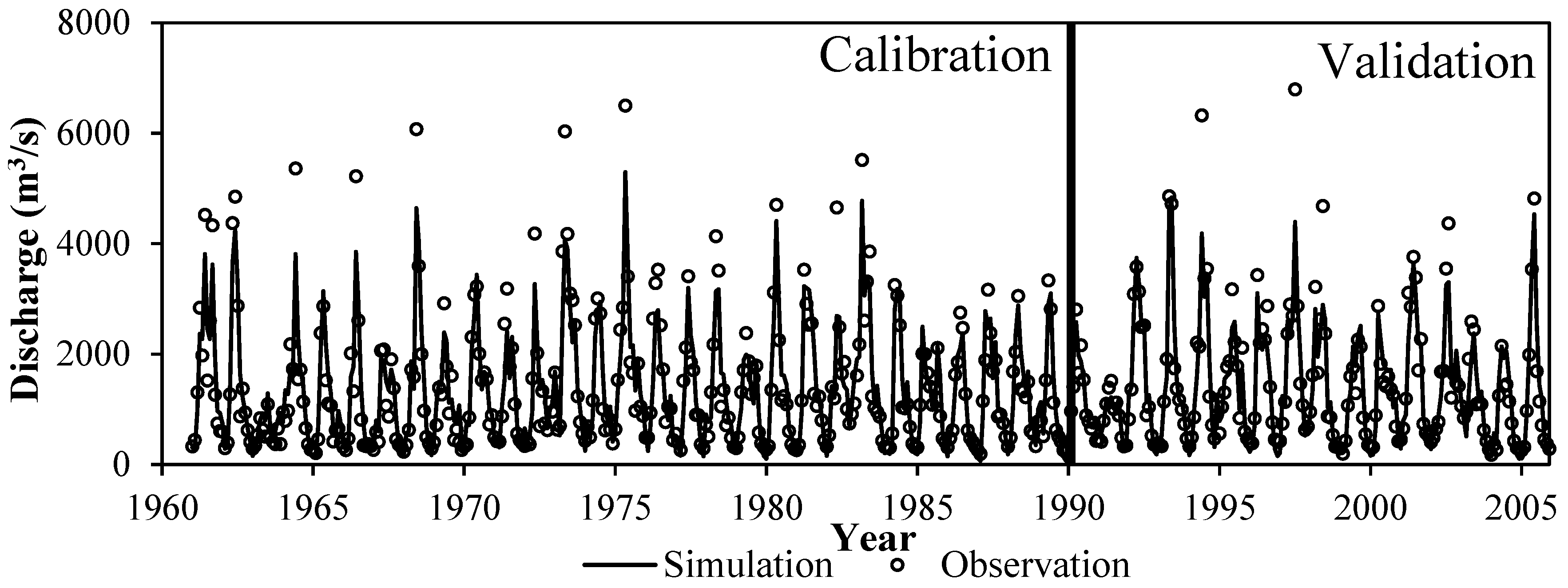
Figure 8.
Predicted LUC of Beijiang River basin in 2050.

Figure 9.
The runoff depth in different months of the dry season under different scenarios.

Figure 10.
Average interannual simulated runoff for the wet year (a), the normal year (b) and the dry year (c) under different LUC scenarios in S2.
Figure 10.
Average interannual simulated runoff for the wet year (a), the normal year (b) and the dry year (c) under different LUC scenarios in S2.
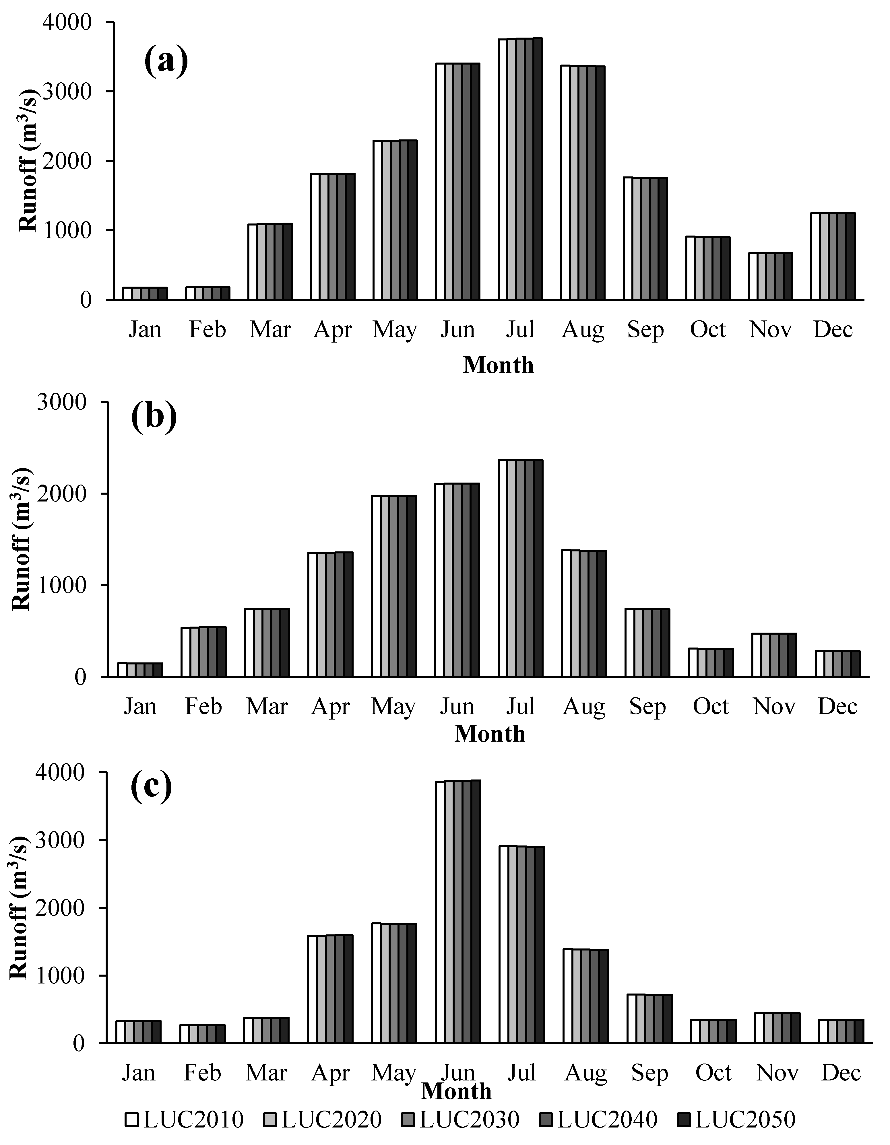
Figure 11.
Changes in runoff components under the different LUC scenarios from 2010 to 2050 in Sub12 (a–c) and Sub31 (d–f). Bar graph shows the annual values, and the triangles show the change percentages between runoff components of LUC2010 and LUC2050. The dash-dotted line shows the horizontal line of the change percentage equaling to 0%.


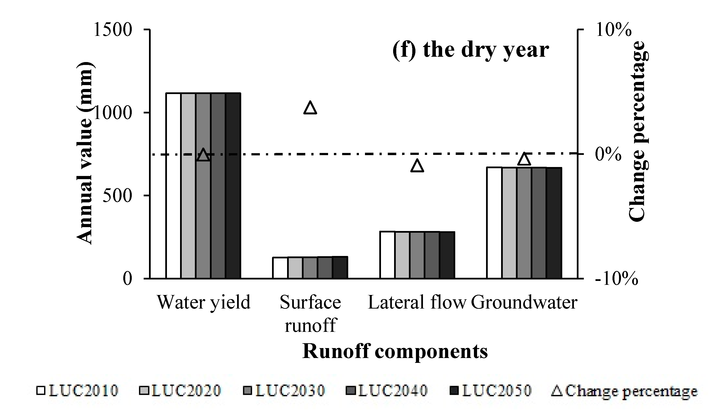
Figure 12.
Average runoff depth at annual (a), and seasonal (wet season (b) and dry season (c)) scales under S3 during 2011–2050.
Figure 12.
Average runoff depth at annual (a), and seasonal (wet season (b) and dry season (c)) scales under S3 during 2011–2050.
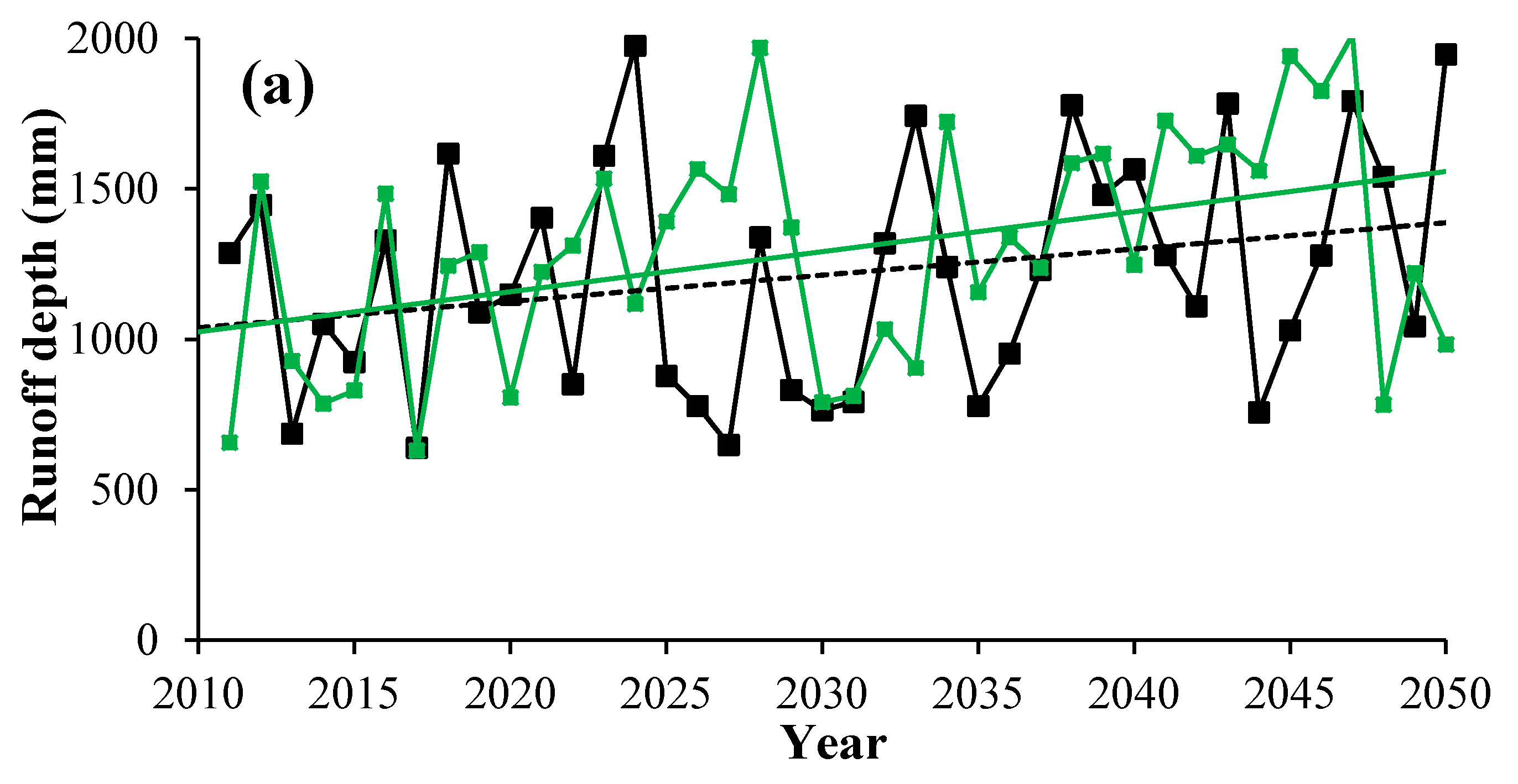

Figure 13.
Average annual runoff components based on S1 and S3 under RCP 4.5 and RCP 8.5 scenarios during the period of 2011–2050.
Figure 13.
Average annual runoff components based on S1 and S3 under RCP 4.5 and RCP 8.5 scenarios during the period of 2011–2050.

Figure 14.
Average annual runoff components based on S2 and S3 during the period of 1961–2010.

Table 1.
Percentages (%) of LUC type in Beijiang River basin.
| LUC Type | The Observed Map | The Predicted Map | |||||
|---|---|---|---|---|---|---|---|
| 1990 | 2000 | 2010 | 2020 | 2030 | 2040 | 2050 | |
| Cropland | 20.8 | 20.8 | 19.4 | 18.8 | 18.6 | 18.4 | 18.3 |
| Forest | 68.2 | 68.1 | 67.5 | 63.6 | 62.7 | 62.1 | 61.7 |
| Orchard | 1.4 | 1.5 | 3.5 | 7.0 | 7.6 | 7.9 | 8.0 |
| Pasture | 6.6 | 6.6 | 5.6 | 5.3 | 5.1 | 4.9 | 4.8 |
| Water body | 1.4 | 1.5 | 1.8 | 2.0 | 2.0 | 2.1 | 2.1 |
| Construction land | 1.6 | 1.6 | 2.2 | 3.3 | 3.9 | 4.5 | 5.1 |
Table 2.
Statistical values of corrections and observations in the calibration period (1961–1990) and validation period (1991–2005).
Table 2.
Statistical values of corrections and observations in the calibration period (1961–1990) and validation period (1991–2005).
| Statistics | Periods | Calibration | Validation | ||||||
|---|---|---|---|---|---|---|---|---|---|
| P (mm/d) | T (°C) | P (mm/d) | T (°C) | ||||||
| QM | Observed | QM | Observed | QM | Observed | QM | Observed | ||
| Mean | Annual | 4.58 | 4.60 | 19.83 | 19.84 | 4.63 | 4.68 | 20.00 | 20.33 |
| Wet | 6.62 | 6.67 | 25.48 | 25.48 | 6.85 | 6.86 | 25.71 | 25.76 | |
| Dry | 2.54 | 2.52 | 14.16 | 14.17 | 2.31 | 2.51 | 14.26 | 14.88 | |
| Standard deviation | Annual | 11.72 | 11.85 | 7.42 | 7.42 | 12.71 | 12.30 | 7.58 | 7.07 |
| Wet | 14.32 | 14.71 | 3.73 | 3.72 | 15.11 | 15.56 | 3.84 | 3.46 | |
| Dry | 7.76 | 7.36 | 5.66 | 5.66 | 7.41 | 7.56 | 5.89 | 5.37 | |
| 95th percentile | Annual | 26.04 | 25.98 | 29.36 | 29.36 | 25.63 | 26.51 | 29.71 | 29.49 |
| Wet | 35.08 | 35.04 | 29.93 | 29.93 | 33.70 | 35.62 | 30.22 | 30.08 | |
| Dry | 14.70 | 14.64 | 23.59 | 23.58 | 13.75 | 14.99 | 24.22 | 23.89 | |
| 75th percentile | Annual | 2.94 | 2.94 | 26.41 | 26.41 | 2.81 | 2.84 | 26.68 | 26.47 |
| Wet | 6.22 | 6.21 | 28.16 | 28.16 | 6.62 | 6.26 | 28.58 | 28.16 | |
| Dry | 1.00 | 1.01 | 18.52 | 18.51 | 0.77 | 0.92 | 19.02 | 18.95 | |
Note: The shaded values indicate that the relative error of statistics between corrections and observations is higher than 5%.
Table 3.
The seasonal change percentages of precipitation (P) and temperature (T) between the future period under RCP4.5 and RCP8.5 and the observations period of 1961–2010.
Table 3.
The seasonal change percentages of precipitation (P) and temperature (T) between the future period under RCP4.5 and RCP8.5 and the observations period of 1961–2010.
| Item | P | T | ||||
|---|---|---|---|---|---|---|
| Annual | Wet | Dry | Annual | Wet | Dry | |
| Change percentage of RCP4.5 | 3% | 6% | −1% | 0.5 °C | 0.7 °C | 1.5 °C |
| Change percentage of RCP8.5 | 8% | 13% | −3% | 1.8 °C | 1.8 °C | 2.0 °C |
Table 4.
Three scenarios for investigating the impacts of climate and LUC changes on the runoff.
| Scenario | Description |
|---|---|
| S1 | Only climate change scenario: RCP4.5 and RCP8.5 (2011–2050). LUC is LUC2010. |
| S2 | Only LUC change scenario: Changing LUC (LUC2010, LUC2020, LUC2030, LUC2040 and LUC2050) with three typical hydrological years. |
| S3 | Simultaneous climate and LUC change scenario in the future: RCP4.5/RCP8.5 (2011–2020) + LUC2020; RCP4.5/RCP8.5 (2021–2030) + LUC2030; RCP4.5/RCP8.5 (2031–2040) + LUC2040; RCP4.5/RCP8.5 (2041–2050) + LUC2050. |
Table 5.
The changes between the predicted runoff depth under RCP 4.5 and RCP 8.5 and the simulated runoff depth during the period of 1961~2005.
Table 5.
The changes between the predicted runoff depth under RCP 4.5 and RCP 8.5 and the simulated runoff depth during the period of 1961~2005.
| Season | Robs (mm) | Rsim (mm) | Prediction under RCP 4.5 | Prediction under RCP 8.5 | ||
|---|---|---|---|---|---|---|
| Change Amount (mm) | Change Percentage (%) | Change Amount (mm) | Change Percentage (%) | |||
| Annual | 1116 | 1118 | +98 | +9 | +178 | +16 |
| Wet | 844 | 836 | +70 | +8 | +144 | +17 |
| Dry | 272 | 282 | +28 | +10 | +34 | +12 |
Note: Robs is the mean value of observed runoff depth during 1961~2005, and Rsim is the mean value of simulated runoff depth based on LUC2010 during 1961~2005. The change amount and change percentage are calculated by comparing Rsim with the predicted runoff depths under RCP 4.5 and RCP 8.5.
Table 6.
Percentages of area (%) of each land use type in Sub12 and Sub31.
| Sub-Watershed | LUC Scenarios | Cropland | Forest | Orchard | Pasture | Water body | Construction Land |
|---|---|---|---|---|---|---|---|
| Sub12 | LUC2010 | 20.1 | 32.9 | 10.6 | 5.0 | 8.9 | 22.5 |
| LUC2020 | 16.2 | 22.8 | 12.5 | 4.6 | 10.3 | 33.6 | |
| LUC2030 | 15.1 | 17.8 | 12.6 | 4.3 | 10.6 | 39.6 | |
| LUC2040 | 15.1 | 17.3 | 12.6 | 4.0 | 10.6 | 40.4 | |
| LUC2050 | 15.2 | 17.0 | 12.1 | 3.9 | 11.1 | 40.7 | |
| Sub31 | LUC2010 | 13.0 | 73.7 | 3.7 | 1.0 | 7.4 | 1.1 |
| LUC2020 | 13.1 | 71.6 | 6.2 | 0 | 7.9 | 1.2 | |
| LUC2030 | 13.1 | 71.4 | 6.4 | 0 | 8.0 | 1.2 | |
| LUC2040 | 13.2 | 71.3 | 6.2 | 0 | 8.0 | 1.4 | |
| LUC2050 | 13.4 | 70.0 | 7.0 | 0 | 8.1 | 1.5 |
© 2017 by the authors. Licensee MDPI, Basel, Switzerland. This article is an open access article distributed under the terms and conditions of the Creative Commons Attribution (CC BY) license (http://creativecommons.org/licenses/by/4.0/).
Share and Cite
MDPI and ACS Style
Pan, S.; Liu, D.; Wang, Z.; Zhao, Q.; Zou, H.; Hou, Y.; Liu, P.; Xiong, L. Runoff Responses to Climate and Land Use/Cover Changes under Future Scenarios. Water 2017, 9, 475. https://doi.org/10.3390/w9070475
AMA Style
Pan S, Liu D, Wang Z, Zhao Q, Zou H, Hou Y, Liu P, Xiong L. Runoff Responses to Climate and Land Use/Cover Changes under Future Scenarios. Water. 2017; 9(7):475. https://doi.org/10.3390/w9070475
Chicago/Turabian StylePan, Sihui, Dedi Liu, Zhaoli Wang, Qin Zhao, Hui Zou, Yukun Hou, Pan Liu, and Lihua Xiong. 2017. "Runoff Responses to Climate and Land Use/Cover Changes under Future Scenarios" Water 9, no. 7: 475. https://doi.org/10.3390/w9070475
Note that from the first issue of 2016, this journal uses article numbers instead of page numbers. See further details here.