Factor Analysis and Estimation Model of Water Consumption of Government Institutions in Taiwan

Abstract

Models for adequately estimating water consumption in Taiwanese government institutions were developed to assist the government to more accurately predict and account for their water needs. A correlation coefficient matrix of associated factors was constructed based on records per unit of water consumption, describing the impact of various water consumption factors. To understand and quantify the effect of the impact factors, linear and nonlinear regression models, as well as an artificial neural network model were adopted. To account for data variability, the data used for modelling were either fully or partially adopted. For partial adoption, the quartile method was employed to remove any outliers. Analysis of the factors affecting water consumption revealed that the building floor area and number of personnel in an organization had the largest impact on estimated consumption, followed by the number of residential personnel. As the coefficient of variation for the green irrigated area and number of consulting personnel was low, the total area and the total number personnel of water consumption decreased the effectiveness of the model.

1. Introduction

The subtropical island nation of Taiwan is affected by monsoons, plum rains, and typhoons. In the northwest Pacific, which is where Taiwan is located, four typhoons occur on average per year. Annual precipitation in Taiwan ranges from 1600 to 3200 mm. Although it is reasonable to expect that Taiwan has abundant fresh water—considering its annual rainfall—70% of precipitation landing on the plains is runoff to the sea and lost to evaporation each year. Most precipitation occurs in summer and autumn, with 78% from plum rains and typhoons between May and October. Additionally, the average annual amount of rainfall per capita in Taiwan is only 4074 m³ as its population density is high at 647 per km², which is low at one-fifth the global rainfall average per capita. Furthermore, the average price of water is USD 0.36 per thousand liters, which is less than 0.1% of the nation’s per capita income. Consequently, the people of Taiwan may take water for granted and not value it as a natural resource [1,2,3] as water consumption per capita in Taipei reaches as high as 335 L per day.

Global warming and climate change are threatening water resources. Given that the volume of reservoirs is limited, much of Taiwan’s terrain is precipitous, and increasingly more areas are being designated as environmental protection areas; thus, balancing the supply of water with demand is becoming more difficult [4,5]. Due to water use in irrigation and filtration, domestic households do not consume the highest percentage of water in Taiwan, but there is still a water shortage crisis. Thus, the promotion of water conservation and the enhancement of water consumption efficiency are indispensable.

To ensure sustainable water consumption, the creation and comparison of different domestic water consumption models may provide a reference for decision-makers in charge of implementing water policy. Therefore, the urgency of a precise water consumption estimation model for government institutions in Taiwan is justified. Water consumption forecasts are affected by numerous factors such as geographical and meteorological phenomena, economic factors, and methods of water consumption. Forecasts simulated using traditional statistical methods may lack sufficient accuracy [6]; however, the water consumption data have a varying range of non-linearity. Therefore, a method or function that does not need specifically structured data is necessary.

The aim of this study was five-fold: (a) to examine the correlation between annual water consumption and the factors affecting water consumption at each government institution; (b) to identify factor differences between different estimation methods; (c) to establish different models suitable for different government institutions; (d) to analyze the accuracies of different water consumption estimation models; and (e) to develop a model that adequately estimates water consumption.

2. Materials and Methods

Related studies can be classified into three major categories: consideration of water consumption impact factors, regression model analyses, and artificial neural network (ANN) analyses.

2.1. Water Consumption Impact Factors

Several studies [6,7,8] have noted the significant impact of various water consumption factors including previous water demand, number of family members, age of family members, garden size, frequency of irrigation, and the water consumption of agriculture.

Previous water consumption data have been considered as the key to estimating future consumption in numerous studies. To manage water consumption effectively, the data of each institution’s water consumption must be collected [9,10]. Creating a suitable model for Taiwanese domestic water consumption requires identifying the major impact factors, thus step-by-step filtering was used in this study to select the major impact factors. Moreover, to avoid multicollinearity problems, all factors were considered in the regression models.

2.2. Regression Model

Numerous studies have employed linear and nonlinear regression to establish water consumption models. Some based on linear regression have included rainfall, air temperature, family income, and the cost of water as independent variables. Regression models have also been used to establish models for related topics such as the water utility market structure [11,12,13,14]. A typical linear regression model of water consumption is expressed as

$$y=c+w_1{x}_1+w_2{x}_2+\cdots +w_P{x}_P$$

(1)

where y is the unit water consumption; w_i is weights; x_i is an impact factor of water consumption; and c is constant. As the model is linear, it is easy to estimate its advantages and disadvantages; however, the true relationships between water consumption and impact factors are not linear, but more complex. Hence, a model using one dependent variable and multiple predictive variables does not yield accurate forecasts. Therefore, nonlinear regression can also be employed

$$y=c·x_1^{C_1}·x_2^{C_2}\cdots x_P^{C_P}$$

(2)

where c_i is the weight of regression. For rapid and convenient calculation, Equation (2) can be reformulated through logarithmic conversion

$$\left(y+\delta \right)=c·{\left(x_1+\delta \right)}^{c_1}·{\left(x_2+\delta \right)}^{c_2}·{\left(x_3+\delta \right)}^{c_3}$$

(3)

or

$$\left(y+\delta \right)=c^{\prime }+c_1·\log \left(x_1+\delta \right)+c_2·\log \left(v_2+\delta \right)+\cdots +c_P·\log \left(v_P+\delta \right)$$

(4)

where $c^{\prime }=\log \left(c\right)$.

2.3. Artificial Neural Networks (ANNs)

Errors are common when traditional forecast methods such as time extrapolation are used. Although widely used in the early 20th century, time extrapolation is rarely used in current studies. ANNs are fast and flexible methods for effectively forecasting domestic water demand [15].

ANNs have been used for estimation models and forecasting in numerous fields. An advantage of ANNs is that they can correlate large and complex datasets [16,17]. An ANN was previously used to develop and assess a drinking water quality model, and a multilayer perceptron ANN was required in the hydrological modelling [18].

2.4. Model of the Current Study

Over the past few decades, there has been a dramatic increase in the published research on sustainable water consumption, with most studies focusing on different industrial contexts. Few studies have discussed water consumption by individual government institutions. Despite the adoption of recent policies in Taiwan aimed at actively promoting water conservation, water demand has not substantially decreased as water consumption efficiency has not been enhanced (

Table 1. Average daily per capita domestic water consumption in Taiwan (2007–2016).

Year	2007	2008	2009	2010	2011	2012	2013	2014	2015	2016	Average in 10 Years
Per capita domestic water consumption (Liter/day)	265	261	258	259	258	257	259	264	263	265	260

Note: Constructed by the authors after review of data from the Water Resource Agency, Ministry of Economic Affairs, Taiwan, ROC.

).

This paper reports the results of a five-phase study that explored the theoretical basis for the estimation model, thus establishing a framework, collecting data, analyzing simulation results, and deriving conclusions. The subjects considered were government institutions located on Taiwan Island, the Penghu Islands, the Kinmen Islands, and the Matsu Islands, all of which have water supplied by faucet. Our data consisted of 2611 units taken from government institution-reported water consumption data since 2006. As there are numerous categories of government institutions in the original database, the categories were divided into 6 primary categories and 47 minor categories (

Table 2. Categories of government institutions.

Primary Categories		Minor Categories			Primary Categories			Minor Categories
No.	Subject	No.	Title	Data Amount	No.	Subject	No.	Title	Data Amount
1	Perform official institution	01	Executive branch	186	3	Investigate training institution	01	Research institution	4
		02	Local government	20			02	Training institution	2
		03	Institution belong local government	114			03	Vocational training center	7
2	Specialized government agencies	01	Tax administration institution	35			04	Other kinds of training center	4
		02	Engineering department	13	4	Medical treatment institution	01	Medical treatment department	39
		03	Court	11			02	Nursing house	18
		04	Security department	25	5	School	01	National school of technology	10
		05	Police office	52			02	National university	15
		06	Library	40			03	Armed and policed school	118
		07	Citizen delegate center	37			04	National senior high school	282
		08	District office	111			05	Public junior high school	933
		09	Household registration office	120			06	Public elementary school	5
		10	Hygiene institution	124			07	Preschool	38
		11	Land administration	48			08	Special education school	14
		12	Election committee	9	6	Other kinds	01	Retail market	16
		13	Weather bureau	9			02	Gymnasium	7
		14	Accident investigation committee	2			03	Prison	30
		15	Veterans service office	15			04	Agricultural institution	9
		16	Airport	9			05	Cleaning squad	20
		17	Funeral institution	2			06	Landfill	1
		18	Other kinds of specialized institution	13			07	Radio	3
		19	Fire bureau	11			08	Other kinds of management institution	10
		20	Police force	4			09	Preparatory office
		21	Cultural center	7					0
		22	Museum	9

). Twenty-two independent variables were adopted in this study (

Table 3. Independent variables adopted in this study.

Code	Independent Variable	Code	Independent Variable
v1	Major institution categories	v12	Usage of simple faucet water
v2	Minor institution categories	v13	Usage of groundwater
v3	Floor space	v14	Usage of rainwater
v4	Irrigate area	v15	Usage of reclaimed water
v5	Number of staff	v16	Usage of other kinds of water
v6	Number of visitor	v17	Unit of faucet water demand
v7	Number of accommodation	v18	Cost of faucet water
v8	With kitchen	v19	Simple faucet water demand
v9	With swimming pool	v20	Groundwater demand
v10	Number of water kinds	v21	Rainwater demand
v11	Usage of faucet water	v22	Reclaimed water demand

).

The original database was sufficiently large to guarantee the accuracy of outlier effect models and data analysis. The quartile outlier method was adopted in this study. Furthermore, linear regression, nonlinear regression, and ANN models were developed by outlier effect models. To accord and compare these models, stepwise regression was used to select an independent variable. Each variable was also chosen to carry out the regression with other variables one by one. The advantage of this approach was that it avoided the problem of multicollinearity in each independent variable, thus preventing unstable regression parameters.

The ANN used in this study was the backpropagation neural network (BPNN), which is the most classic and general training algorithm. It also effectively solves problems including multilayers, feed-forwards, and supervised learning functions for different industries [19]. A constructive algorithm was used to determine the number of neurons in the hidden layer, which was initially set to one and gradually incremented until the most suitable number was determined [20]. The output was then expressed as

$$Z_k=f\left(b_{0k}+{\displaystyle \sum }_{j=1}^J{b}_{jk}·f\left(a_{0j}+{\displaystyle \sum }_{i=1}^I{a}_{ij}·x_i\right)\right)$$

(5)

where $f(·)$ is a transfer function; $x_i$ is the input; $a_{ij}$ and $b_{jk}$ are the weights; and $a_{0j}$ and $b_{0k}$ are the bias. The function $f(·)$ is a mapping rule for converting input into output. The most commonly adopted nonlinear conversion function in BPNN studies is the binary logistic sigmoid

$$f\left(x\right)=\frac{1}{1+e^{-x}}$$

(6)

where $f\left(x\right)=\left[0,1\right]$. To obtain more optimal BPNN parameters, $Z_k$ (output value) and $t_k$ (target value) are adjusted through

$$E=\frac{1}{2}{\displaystyle \sum }_{k=1}^K{\left(Z_k-t_k\right)}^2$$

(7)

BPNN uses the method of gradient descent to train all the examples during each learning epoch and obtains the weights $a_{ij}$ and $b_{jk}$. The results obtained during the learning epoch are then fed back into the hidden layer to increase accuracy. Accordingly,

$$\frac{\partial E}{\partial b_{jk}}=\frac{\partial E}{\partial z_k}·\frac{\partial z_k}{\partial v_k}·\frac{\partial v_k}{\partial b_{jk}}$$

(8)

where $\partial E/\partial z_k=\left(z_k-t_k\right)$, $z_k=f\left(v_k\right)$. Thus, $\partial z_k/\partial v_k=f^{\prime }\left(v_k\right)$.

As $v_k=b_{0k}+{\sum }_{j=1}^J{b}_{jk}·y_j$, $\partial v_k/\partial b_{jk}=1\left(j=0\right)$ or $y_j\left(j=1,2,\cdots ,J\right)$, Equation (8) can be differentiated as

$$\frac{\partial E}{\partial a_{ij}}=\left({\displaystyle \sum }_{k=1}^K\frac{\partial E}{\partial z_k}\right)·\frac{\partial y_j}{\partial u_j}·\frac{\partial u_j}{\partial a_{ij}}$$

(9)

where $y_j=f\left(u_j\right)$; thus, $\partial y_j/\partial u_j=f^{\prime }\left(u_j\right)$. The weights can be determined using Equations (8) and (9). When gradient descent was used, a common problem was that convergence did not feedback to the whole network, but only a partial network. To increase learning rate and accuracy, a momentum term was added to avoid oscillation during convergence. The mth weight can be expressed as

$$\Delta w^m=-\eta ·\frac{\partial E}{\partial w^m}+\alpha ·\Delta w^{m-1}$$

(10)

where $\eta$ is the learning rate of the gradient descent method; and $\alpha$ is the momentum factor. To fit the range of the transport function, data were normalized using the max–min mapping method. For a minimum and maximum of the transport function $f_{min}$ and $f_{max}$, the minimum and maximum inputs in the database were $x_{min}$ and $x_{max}$, respectively

$$x^{\left(s\right)}=\zeta ·\left[f_{min}+\frac{x-x_{min}}{x_{max}-x_{min}} \left(f_{max}-f_{min}\right)\right]$$

(11)

where $\zeta$ is the normalized factor. Equation (11) can be reversed as

$$\widehat{x}=x_{min}+\frac{\left({\widehat{x}}^{\left(s\right)}/\zeta \right)-f_{min}}{f_{max}-f_{min}}\times \left(x_{max}-x_{min}\right)$$

(12)

where ${\widehat{x}}^{\left(s\right)}$ and $\widehat{x}$ are estimates of $x^{\left(s\right)}$ and x, respectively.

2.5. Model Efficiency Indexes

A comparison of three methods was adopted, where the R² of ANN was obviously the highest. However, judging which method was more suitable via R² was far from enough. Five model efficiency indices were employed to determine the suitability of each model: the mean absolute deviation (MAD), root mean squared error (RMSE), revised Teil inequality coefficient (RTIC), correlation coefficient (CC), and coefficient of efficiency (CE), defined as

$$MAD=\frac{1}{N}{\displaystyle \sum }_{i=1}^N\left|Q_i-{\widehat{Q}}_i\right|$$

(13)

where N is the total number of units; $Q_i$ is the real water consumption; and ${\widehat{Q}}_i$ is the estimated water consumption.

$$RMSE=\sqrt{\frac{{\sum }_{i=1}^N{\left(Q_i-\widehat{Q}\right)}^2}{N}}$$

(14)

$$RTIC=\sqrt{\frac{{\sum }_{i=1}^N{\left(Q_i-{\widehat{Q}}_i\right)}^2}{{\sum }_{i-1}^N{\left(Q_i\right)}^2}}$$

(15)

$$CC=\frac{{\sum }_{i=1}^N\left(Q_i-{\overline{Q}}_i\right)\left({\widehat{Q}}_i-\overline{{\widehat{Q}}_i}\right)}{\sqrt{{\sum }_{i=1}^N{\left(Q_i-{\overline{Q}}_i\right)}^2·{\sum }_{i=1}^N{\left({\widehat{Q}}_i-\overline{{\widehat{Q}}_i}\right)}^2}}$$

(16)

where ${\overline{Q}}_i$ is the mean of $Q_i$; and $\overline{{\widehat{Q}}_i}$ is the mean of ${\widehat{Q}}_i$.

$$CE=1-\frac{{\sum }_{i=1}^N{\left(Q_i-{\widehat{Q}}_i\right)}^2}{{\sum }_{i=1}^N{\left(Q_i-{\overline{Q}}_i\right)}^2}$$

(17)

Of the five efficiency indices, MAD, RMSE, and RTIC indicated higher efficiency as they approached zero. As CC approached one, the simulated and actual values became more closely correlated, whereas CE approaching one indicated higher precision.

3. Results

For multiple regression models, selecting suitable factors that were consistent and comparable was crucial; thus, each water consumption factor was tested against the water consumption data through a correlation analysis. The top six correlations between v17 and other water consumption factors were: v18, v05, v03, v07, v09, and v06. As v18 was converted from v17, it was not included in the analysis. Given that collinearity in the design matrix can result in inaccurate regression model estimates, v19 and v21 were excluded from the initial estimations due to the high collinearity between v19, v21, and v05. Usage of faucet water (v11) was one for all working databases; therefore, v11 was also eliminated.

Through step-by-step filtering, independent variables that failed a t test (i.e., t = 1.96) were eliminated one by one. The linear regression and nonlinear regression models developed in this study, which considered 2611 data inputs, are shown in Equations (18) and (19), respectively

$$v_{17}=c+c_3{v}_3+c_4{v}_4+c_5{v}_5+c_6{v}_6+c_7{v}_7+c_8{v}_8+c_9{v}_9+c_{13}{v}_{13}+c_{15}{v}_{15}$$

(18)

$$\left(v_{17}+\delta \right)=c·{\left(v_3+\delta \right)}^{c_3}·{\left(v_4+\delta \right)}^{c_4}·{\left(v_5+\delta \right)}^5·{\left(v_6+\delta \right)}^{c_6}·{\left(v_7+\delta \right)}^{c_7}·{\left(v_9+\delta \right)}^{c_9}·{\left(v_{13}+\delta \right)}^{c_{13}}·{\left(v_{15}+\delta \right)}^{c_{15}}$$

(19)

The R of these models was 0.665 and 0.692, respectively.

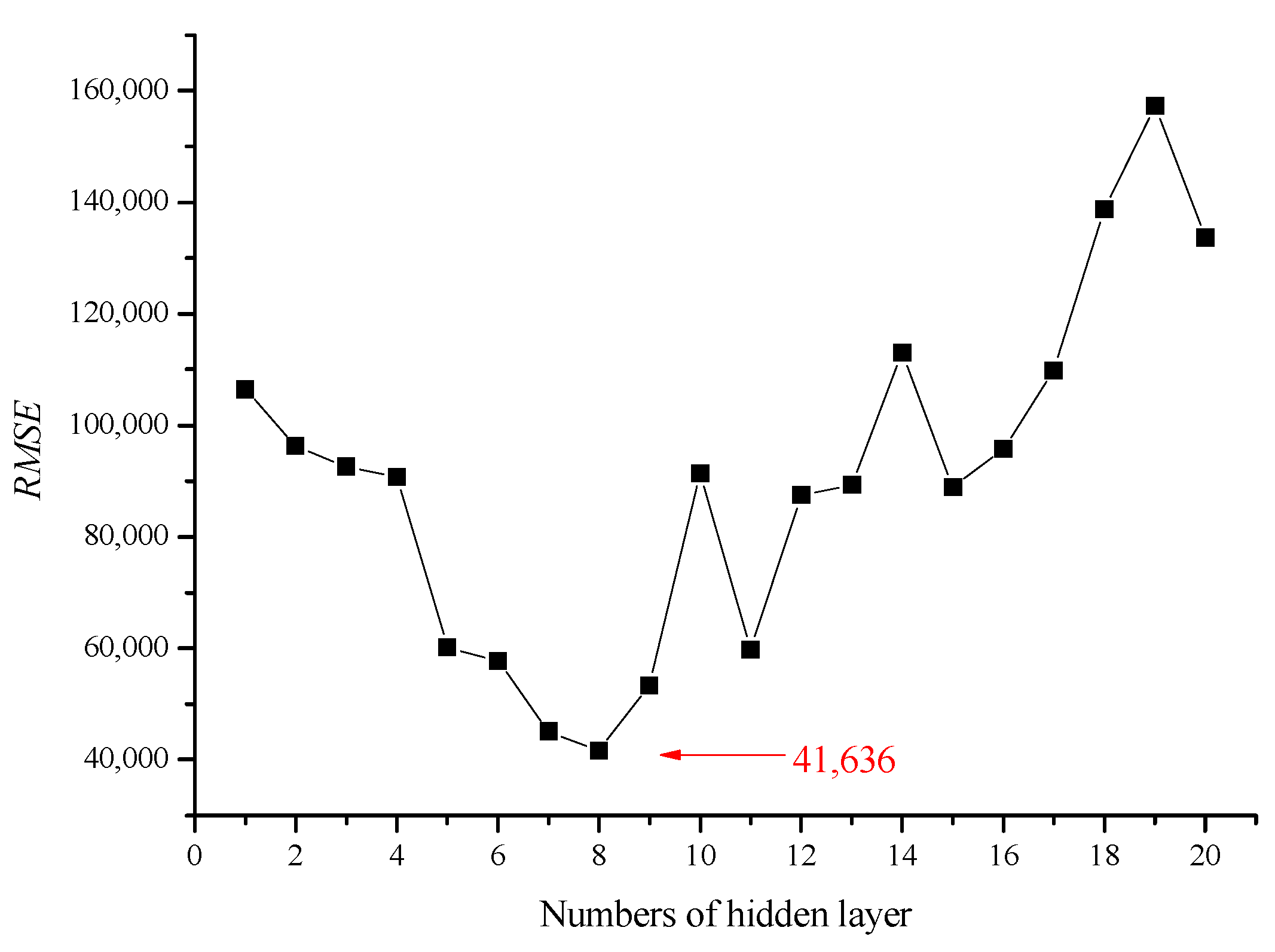
When the ANN was employed to simulate the models, 100 random data inputs were sampled to act as a verification sample. The number of hidden layers was determined through trial and error, with the minimum number from 1 to 20, which was calculated from [(input layer = 9) + (output layer = 1)] × 2. To determine the lowest RMSE and highest R, a constructive algorithm was used. Eight hidden layers were found to result in the lowest RMSE, as depicted in Figure 1. The R and RMSE in this model were 0.929 and 41,636, respectively.

Due to the possible typographical errors in the data used in this study, outliers for water demand per floor space unit (q_A), water demand per number of staff (q_N), and water demand per number of staff and per floor space (q_AN) were considered. The quartile outlier method was employed for q_A data, with the linear regression model

$$v_{17}=c+c_3{v}_3+c_4{v}_4+c_5{v}_5+c_6{v}_6+c_7{v}_7+c_9{v}_9+c_{13}{v}_{13}$$

(20)

The R of this linear regression model for deducting outliers under q_A was 0.710. Equation (20) was then modified to an improved nonlinear regression model

$$\log \left(v_{17}+\delta \right)=\acute{c}+c_3·\log \left(v_3+\delta \right)+c_4·\log \left(v_4+\delta \right)+c_5·\log \left(v_5+\delta \right)+c_6·\log \left(v_6+\delta \right)+c_7·\log \left(v_7+\delta \right)+c_9·\log \left(v_9+\delta \right)+c_{13}·\log \left(v_{13}+\delta \right)$$

(21)

The R of this nonlinear regression model for deducting outliers under q_A was 0.699. In the eight hidden layers of the ANN, the R was 0.904. Regarding the aforementioned quartile outlier method, the outliers under q_N were deducted. With this condition, the linear regression, nonlinear regression, and ANN models were obtained. The linear regression model for deducting outliers under q_N is shown in Equation (22), and the resultant R was 0.773

$$v_{17}=c+c_3{v}_3+c_4{v}_4+c_5{v}_5+c_6{v}_6+c_7{v}_7+c_{13}{v}_{13}$$

(22)

The nonlinear regression model for deducting outliers under q_N is shown in Equation (23), and the resultant R was 0.738

$$\log \left(v_{17}+\delta \right)=\acute{c}+c_3·\log \left(v_3+\delta \right)+c_4·\log \left(v_4+\delta \right)+c_5·\log \left(v_5+\delta \right)+c_6·\log \left(v_6+\delta \right)+c_7·\log \left(v_7+\delta \right)+c_{13}·\log \left(v_{13}+\delta \right)$$

(23)

Under this condition, with eight hidden ANN layers, the R was 0.953.

Furthermore, outliers under q_AN were considered. With the quartile outlier method, the linear regression model was found to be identical to Equation (22), with R = 0.688. Similarly, the nonlinear regression model was identical to Equation (23), with R = 0.720. Eight was again, the most suitable number of hidden layers, and R was 0.866.

As previously mentioned, full adoption and partial adoption models were estimated. Given that the quartile outlier method for partial adoption is similar to that used to estimate the energy usage index in Taiwan, the use of raw water demand data to establish a model of water consumption was found to be unsuitable. Therefore, the outliers determined in the water demand per floor space unit, water demand per number of staff, and water demand per number of staff and per floor space unit were ignored. This outlier removal method was expected to improve the accuracy of the established water consumption model.

Table 4. Performance comparison of each water demand model with full or partial adoption.

Data	Model	MAD	RMSE	RTIC	CC	CE
Full adoption	Linear regression	9,020.42	92,010.83	0.7153	0.6657	0.4431
	Non-linear regression	6,890.49	31,581.66	0.7058	0.6917	0.4580
	ANN	5,591.42	15,936.16	0.3561	0.9285	0.8620
Exclude outlier of qA	Linear regression	6,547.07	22,858.52	0.6693	0.7098	0.5037
	Non-linear regression	5,172.72	24,286.02	0.7111	0.6985	0.4398
	ANN	4,652.40	13,857.35	0.4057	0.9043	0.8176
Exclude outlier of qN	Linear regression	5,633.69	16,870.19	0.5967	0.7730	0.5973
	Non-linear regression	4,453.26	18,383.52	0.6503	0.7375	0.5219
	ANN	3,734.64	8,083.06	0.2859	0.9528	0.9076
Exclude outlier of qAN	Linear regression	9,033.15	31,288.56	0.6931	0.6879	0.4732
	Non-linear regression	7,013.14	31,088.85	0.6887	0.7201	0.4799
	ANN	6,867.00	21,605.54	0.4786	0.8662	0.7488

Notes: q_A = Total area of water consumption, q_N = Total number personnel of water consumption, q_AN = Water demand of per number of personnel times per floor space unit.

details the performance of each water demand model for full and partial adoptions, with the linear regression, nonlinear regression, and ANN models employed. Five efficiency indices were used to gauge model performance. The ANN model with outlier removal under water demand per number of staff was the most accurate model for estimating water consumption by government institutions in Taiwan, demonstrating the closest fit to the actual data. Considering all five model efficiency indices, the descending order of efficiency of these approaches was as follows: Excluding outliers under q_N > excluding outliers under q_A > excluding outliers under q_AN > full adoption. The total efficiency for q_AN was low due to a factor multiplication effect (vA = v03 + v04; vN = v05 + v06 + v07).

Considering the MAD index, all three models were more accurate when the quartile outlier method was implemented to remove outliers under q_N. The RMSE for the nonlinear regression model was higher than that for the linear regression model, which might be attributable to the nonlinear regression model being reversed and any deviation thus being increased. For the RTIC index, which indicates higher precision as it approaches 0, the ANN model was identified as the most efficient. The q_N ANN model was also the most precise model when the RTIC index was considered. The CC index of the q_N ANN model was 0.9528, which was the highest among all the models. Therefore, outlier removal under q_N using an ANN was the most suitable model for estimating water consumption.

4. Conclusions

The data employed in this study concerned the water consumption of all government institutions in Taiwan. Linear regression, nonlinear regression, and an ANN were adopted to establish a water consumption estimation model. The quartile outlier method was also used to determine the effect on prediction accuracy for full or partial adoption of data. The major factors influencing water consumption were divided into four categories: area of water demand (floor and irrigation areas); water demand population (number of staff, visitor, and accommodation); usage of equipment with high water consumption (kitchens and swimming pool); and usage of non-faucet water sources (i.e., groundwater). In each case, the removal of outliers under q_N with an ANN was the most accurate model. Furthermore, adopting the quartile outlier method maintained the median and effectively decreased data variability.

The school (education) category was identified as consuming the most water. The total number of school category was 1415, which accounted for most of the database in this study. Educational institutions were the best fit and the model used for other types of institutions, therefore, the model was most suitable when q_N outliers were identified because the q_N ANN model was the most suitable for fitting within the school category. An improved model that considered other categories could be established if more complete data on other institutions were available. A classic and general ANN model was employed in this study; thus, the activation function and number of hidden layers may also have affected its efficiency and precision.

The models established in this study could form the review process when each government institution imports their variable data in that year. Therefore, estimated water consumption can be calculated and used to judge whether the water consumption of government institutions is deemed reasonable. Hence, the established models could be the evaluation for saving water.

References

- Peng, T.R.; Lu, W.C.; Chen, K.Y.; Zhan, W.J.; Liu, T.K. Groundwater-recharge connectivity between a hills-and-plains’ area of western Taiwan using water isotopes and electrical conductivity. J. Hydrol. 2014, 517, 226–235. [Google Scholar] [CrossRef]
- Chen, Y.C.; Chang, K.T.; Lee, H.Y.; Chiang, S.H. Average landslide erosion rate at the watershed scale in southern Taiwan estimated from magnitude and frequency of rainfall. Geomorphology 2015, 228, 756–764. [Google Scholar] [CrossRef]
- Shiau, J.T.; Huang, W.H. Detecting distributional changes of annual rainfall indices in Taiwan using quantile regression. J. Hydro-Environ. Res. 2014, 9, 1053–1069. [Google Scholar] [CrossRef]
- Cheng, F.Y.; Jian, S.P.; Yang, Z.M.; Yen, M.C.; Tsuang, B.J. Influence of regional climate change on meteorological characteristics and their subsequent effect on ozone dispersion in Taiwan. Atmos. Environ. 2015, 103, 66–81. [Google Scholar] [CrossRef]
- Chou, K.T. The public perception of climate change in Taiwan and its paradigm shift. Energy Policy 2013, 61, 1252–1260. [Google Scholar] [CrossRef]
- Keshavarzi, A.R.; Sharifzadeh, M.; Kamgar Haghighi, A.A.; Amin, S.; Keshtkar, S.; Bamdad, A. Rural domestic water consumption behavior: A case study in Ramjerd area, Fars province, I.R. Iran. Water Res. 2006, 40, 1173–1178. [Google Scholar] [CrossRef] [PubMed]
- Romano, M.; Kapelan, Z. Adaptive water demand forecasting for near real-time management of smart water distribution systems. Environ. Model. Softw. 2014, 60, 265–276. [Google Scholar] [CrossRef]
- Thevs, N.; Nurtazin, S.; Beckmann, V.; Salmyrzauli, R.; Khalil, A. Water Consumption of Agriculture and Natural Ecosystems along the Ili River in China and Kazakhstan. Water 2017, 9, 207. [Google Scholar] [CrossRef]
- Angelakis, A. Evolution of rainwater harvesting and use in Crete, Hellas, through the millennia. Water Sci. Technol. 2016, 16, 1624–1638. [Google Scholar] [CrossRef]
- Shrestha, S.; Aihara, Y.; Bhattarai, A.P.; Bista, N.; Rajbhandari, S.; Kondo, N.; Kazama, F.; Nishida, K.; Shindo, J. Dynamics of Domestic Water Consumption in the Urban Area of the Kathmandu Valley: Situation Analysis Pre and Post 2015 Gorkha Earthquake. Water 2017, 9, 222. [Google Scholar] [CrossRef]
- Bakker, M.; van Duist, H.; van Schagen, K.; Vreeburg, J.; Rietveld, L. Improving the performance of water demand forecasting models by using weather input. Procedia Eng. 2014, 70, 93–102. [Google Scholar] [CrossRef]
- Chen, Z.; Ngo, H.H.; Guo, W.; Wang, X.C.; Miechel, C.; Corby, N.; Listowski, A.; O’Halloran, K. Analysis of social attitude to the new end use of recycled water for household laundry in Australia by the regression models. J. Environ. Manag. 2013, 126, 79–84. [Google Scholar] [CrossRef] [PubMed]
- Carvalho, P.; Marques, R.C.; Berg, S. A meta-regression analysis of benchmarking studies on water utilities market structure. Util. Policy 2012, 21, 40–49. [Google Scholar] [CrossRef]
- Candelieri, A. Clustering and Support Vector Regression for Water Demand Forecasting and Anomaly Detection. Water 2017, 9, 224. [Google Scholar] [CrossRef]
- Lin, Y.; Li, Q.; Li, X.; Ji, K.; Zhang, H.; Yu, Y.; Song, Y.; Fu, Y.; Sun, L. Pyrolysates distribution and kinetics of Shenmu long flame coal. Energy Convers. Manag. 2014, 86, 428–434. [Google Scholar] [CrossRef]
- Trichakis, I.C.; Nikolos, I.K.; Karatzas, G. Artificial neural network (ANN) based modeling for karstic groundwater level simulation. Water Resour. Manag. 2011, 25, 1143–1152. [Google Scholar] [CrossRef]
- Afan, H.A.; El-Shafie, A.; Yaseen, Z.M.; Hameed, M.M.; Mohtar, W.H.M.W.; Hussain, A. ANN based sediment prediction model utilizing different input scenarios. Water Resour. Manag. 2015, 29, 1231–1245. [Google Scholar] [CrossRef]
- Zangooei, H.; Delnavaz, M.; Asadollahfardi, G. Prediction of coagulation and flocculation processes using ANN models and fuzzy regression. Water Sci. Technol. 2016, 74, 1296–1311. [Google Scholar] [CrossRef] [PubMed]
- Huang, H.X.; Li, J.C.; Xiao, C.L. A proposed iteration optimization approach integrating backpropagation neural network with genetic algorithm. Expert Syst. Appl. 2015, 42, 146–155. [Google Scholar] [CrossRef]
- Lan, Y.; Soh, Y.C.; Huang, G.B. Constructive hidden nodes selection of extreme learning machine for regression. Neurocomputing 2010, 73, 3191–3199. [Google Scholar] [CrossRef]
Figure 1.
RMSE for various numbers of hidden layers.