Mapping Submerged Aquatic Vegetation Using RapidEye Satellite Data: The Example of Lake Kummerow (Germany)
by
 , , and
Christine Fritz
1,*, 
Katja Dörnhöfer
2,
Thomas Schneider
1,
Juergen Geist
1 and
Natascha Oppelt
2 1
Aquatic Systems Biology Unit, Limnological Research Station Iffeldorf, Department of Ecology and Ecosystem Management, Technical University of Munich, Hofmark 1–3, 82393 Iffeldorf, Germany
2
Earth Observation and Modelling, Department of Geography, Christian-Albrechts-Universität zu Kiel, Ludewig-Meyn-Str. 14, 24098 Kiel, Germany
*
Author to whom correspondence should be addressed.
Water 2017, 9(7), 510; https://doi.org/10.3390/w9070510
Submission received: 20 March 2017
/
Revised: 13 June 2017
/
Accepted: 5 July 2017
/
Published: 12 July 2017
(This article belongs to the Special Issue Water Quality Monitoring and Modeling in Lakes)
Abstract
:Submersed aquatic vegetation (SAV) is sensitive to changes in environmental conditions and plays an important role as a long-term indictor for the trophic state of freshwater lakes. Variations in water level height, nutrient condition, light availability and water temperature affect the growth and species composition of SAV. Detailed information about seasonal variations in littoral bottom coverage are still unknown, although these effects are expected to mask climate change-related long-term changes, as derived by snapshots of standard monitoring methods included in the European Water Framework Directive. Remote sensing offers concepts to map SAV quickly, within large areas, and at short intervals. This study analyses the potential of a semi-empirical method to map littoral bottom coverage by a multi-seasonal approach. Depth-invariant indices were calculated for four Atmospheric & Topographic Correction (ATCOR2) atmospheric corrected RapidEye data sets acquired at Lake Kummerow, Germany, between June and August 2015. RapidEye data evaluation was supported by in situ measurements of the diffuse attenuation coefficient of the water column and bottom reflectance. The processing chain was able to differentiate between SAV and sandy sediment. The successive increase of SAV coverage from June to August was correctly monitored. Comparisons with in situ and Google Earth imagery revealed medium accuracies (kappa coefficient = 0.61, overall accuracy = 72.2%). The analysed time series further revealed how water constituents and temporary surface phenomena such as sun glint or algal blooms influence the identification success of lake bottom substrates. An abundant algal bloom biased the interpretability of shallow water substrate such that a differentiation of sediments and SAV patches failed completely. Despite the documented limitations, mapping of SAV using RapidEye seems possible, even in eutrophic lakes.
1. Introduction
Monitoring submersed aquatic vegetation (SAV) is important, since occurrence and species composition are long-term indicators for the trophic state of freshwater ecosystems [1]. SAV is sensitive to nutrient conditions, water temperature, water level and transparency [2,3,4,5]. Changing water temperatures can induce changes in plant species composition, expansion, and date of vegetation emergence and senescence [6,7,8]. SAV is one of the biological quality elements (BQE) used in monitoring the ecological status of surface waters within the process recommended by the European Water Framework Directive (WFD). The present regulation requires mapping on a species level every third year, preferably by divers [9]. Global change affects ecological balance in freshwater lakes. To detect changes at an early stage, Palmer et al. [10] recommended more frequent observations of freshwater lakes. Remote sensing provides time- and cost-effective methods to observe seasonal and annual changes in water quality and macrophyte coverage [11,12,13,14,15,16,17,18,19]. Palmer et al. [10] concluded that changes in SAV covered areas can be detected by recently available remote sensing systems that are well suited to complement regular in situ sampling, as required by the WFD. The approach is expected to bridge observation gaps between snapshots of in situ mappings [10,20]. High revisiting time and broad coverage of shallow lakeshore areas of remote sensing data may compensate for the reduced information on species compared to mappings.
The information provided by remote sensing relies on the interpretability of spectral signatures delivered by the employed systems. The vegetation/sediment ratio controls the spectral response from the lake bottom. At the beginning of the growing season, sediment dominates the spectral response. During this period, the organic overlay on the sediment such as detritus or epiphytes modifies the spectral response of the pure sediment [6,15,21,22,23]. SAV displays a highly dynamic appearance within the short vegetation period, which lasts approximately from mid-June to mid-September. Along with SAV growth, the spectral signature of the SAV changes. Varying leaf size, leaf orientation, pigment content and ratio within the vegetation period influence signal intensity and shape [6,15,22]. After bottom coverage and biomass are at a maximum, the senescence phase begins. Pigment degradation and canopy structural changes characterize this stage [15], especially the degradation of chlorophyll a (Chl a) content in ageing leaves affects the spectral signature [24,25]. The results from Pinnel et al. [18] and Wolf et al. [15] indicated that the different developmental patterns of competing macrophyte species along the vegetation period may be the key for differentiation on a species level.
Hyperspectral imaging at close intervals along the vegetation period is best suited to provide necessary spectral information [18,19,26,27,28]. Nevertheless, operational monitoring as required by the WFD, needs high revisiting frequencies and large area coverage. Costs associated with hyperspectral imaging hinder such an approach. Palmer et al. [10], Roessler et al. [19] and Dekker et al. [26] suggested using multi-seasonal imaging by high spatial resolution multispectral satellite data in order to compensate for the reduced spectral information.
Multi-seasonal imaging is inevitably connected to the need to provide comparable data sets over time. This means that external factors influencing the spectral signal have to be corrected, i.e., changes in the atmosphere, water column and lake surface.
A freely available, sensor-generic atmospheric correction algorithm for freshwater body correction is presently not available. For freshwater, atmospheric algorithms of land applications therefore are a trade-off between availability and accuracy of results. A widely used software is Atmospheric & Topographic Correction (ATCOR2) [29], which proved to be helpful in the case of airborne hyperspectral data evaluations for water depth estimation [30], for water constituents and littoral bottom mapping [27], but also for mapping SAV [31] with RapidEye data [19].
Water constituents differ among water bodies and may change rapidly in concentration and composition within a water body. In combination with varying water depths, they strongly affect the signal. Different strategies exist to consider the attenuation by the water column, particularly bio-optical and semi-empirical modelling [28,32,33,34,35]. While bio-optical model inversion on the front end of water content and bottom type determination rely on sample spectra, semi-empirical modelling may be operated without such ‘a-priori’ information. Previous studies revealed that depth-invariant indices provide a possibility for the detection and distinguishing of bottom coverage of lakes and shorelines. Armstrong [23] mapped seagrass and estimated its biomass at the shallow water areas in the Bahamas using Landsat Thematic Mapper in combination with field surveys and plant collection. Manessa et al. [36] analysed WorldView2 imagery to study the distribution of seagrass and corals of shallow water coral reefs in Indonesia. Ciraolo et al. [37] used the airborne Multispectral Infrared Visible Imaging Sensor (MIVIS) to detect the distribution of seagrass (Posidonia oceanica) in a coastal lagoon in Italy. To assess the littoral bottom coverage of inland waters, Brooks et al. [38] and Shuchman et al. [39] investigated SAV (notably Cladophora spec.) at the Laurentian Great Lakes. They used a depth-invariant SAV mapping algorithm [39] using Landsat Thematic Mapper and Multispectral Scanner Imagery time series from the mid-1970s to 2012. Roessler et al. [19] applied depth-invariant indices to detect and distinguish SAV (Elodea nuttallii and Najas marina) at Lake Starnberg (Germany) using a time series of multispectral RapidEye data.
Varying expansion behaviour in successive years due to shifts in vegetation periods, different water clarity, nutrient loading and lake substrate remobilization processes [26] may influence detectability of SAV, all of which are unpredictable factors exacerbated by global warming. RapidEye data time series seem well appropriated for seasonal SAV mapping. The five-identical-system-constellation promises frequent observation opportunities, a prerequisite for phenologic change observations within the vegetation period.
The present study had the core objective of testing the applicability of RapidEye satellite systems with their high spatial and low spectral resolution, to map SAV in shallow areas of freshwater lakes in a multi-seasonal approach. While in previous studies, oligotrophic lakes were investigated [18,19,28] in this case study, Lake Kummerow, a eutrophic lake in Mecklenburg-Western Pomerania (MV), North-East Germany, was chosen. A semi-empirical method by Lyzenga [33,35] was used to correct the influence of the water column in the RapidEye time series during the vegetation period from June to August 2015.
2. Materials and Methods
2.1. Study Site
Lake Kummerow (53.808° N, 12.856° E) is a eutrophic lake, which developed as a proglacial lake in Germany’s Northern Lowland during the last ice age. Its wind-exposed location and relatively shallow depth (average depth: 8.1 m, maximum depth: 23.3 m) determine its polymictic mixing character [40]. Sandy or muddy sediments dominate the substrate. Wöbbecke et al. [40] described that macrophytes had disappeared in the 1960s. Detailed mappings of lakeshore vegetation and submersed macrophytes were lacking until the 2000s. With the implementation of WFD, in situ mappings along transects were conducted in the years 2003, 2007, 2008, 2009, 2011 and 2013. These inventories revealed the existence of different macrophyte populations in Lake Kummerow. In 2013, the growth limit was, on average, down to a depth of 2.5 ± 0.4 m from the surface at the 15 transects mapped ([41], Figure 1). Potamogeton pectinatus predominates macrophyte coverage in the northern part of the lake. The southern part shows a wider variety of pondweeds such as Potamogeton pectinatus, Potamogeton perfoliatus, Ceratophyllum demersum, Myriophyllum spicatum, and singularly occurring species (Elodea canadensis, Myriophyllum alterniflorum, Myriophyllum spicatum, Potamogeton obtusifolius und Potamogeton friesii). The overall evaluation of Lake Kummerow’s ecological status, performed with the software PHYLIB (version 4.1) [42] based on the BQE macrophytes, revealed a ‘poor ecological status’ for the year 2013 [41].
2.2. Data Collection and Processing
Between June and August, we conducted several measurement campaigns at Lake Kummerow aiming to validate water quality from RapidEye satellite imagery. In situ measurements included water sample analyses and radiometric measurements with two submersible RAMSES spectroradiometers [43] at three to five sites in optically deep water, i.e., where the bottom was not visible (Figure 1). A Trimble Juno SB GPS device (2–5 m positional accuracy, [44]) tracked global positioning system (GPS) coordinates of measurement sites during data acquisition. The measurement setup consisted of a floating frame in which both sensors were mounted on a depth adjustable bar so that the detectors were always at the same water depth (). One sensor (ARC-VIS) measured upwelling radiance, [W m−2 nm−1 sr−1], while the other sensor (ACC-VIS) measured downwelling hemispherical irradiance [W m−2 nm−1], at two depths below water, i.e., −0.21 m () and −0.67 m (). At each measurement point, the ACC-VIS sensor was lifted above the water surface for one additional measurement of . The sensors collected radiometric data between 325 nm and 900 nm in 3.3 nm intervals. Single measurements were linearly interpolated to 1 nm intervals. Remote sensing reflectance [sr−1] was calculated according to Equation (1) [45].
For determining the water-leaving radiance, , measurements from the two depths were linearly extrapolated to just beneath the water surface using the attenuation coefficient of upwelling radiance () [m−1] and corrected for air-water interface [45]; =constant = 0.54, = refractive index of water, t = Fresnel reflectance of air-water interface; Equation (2).
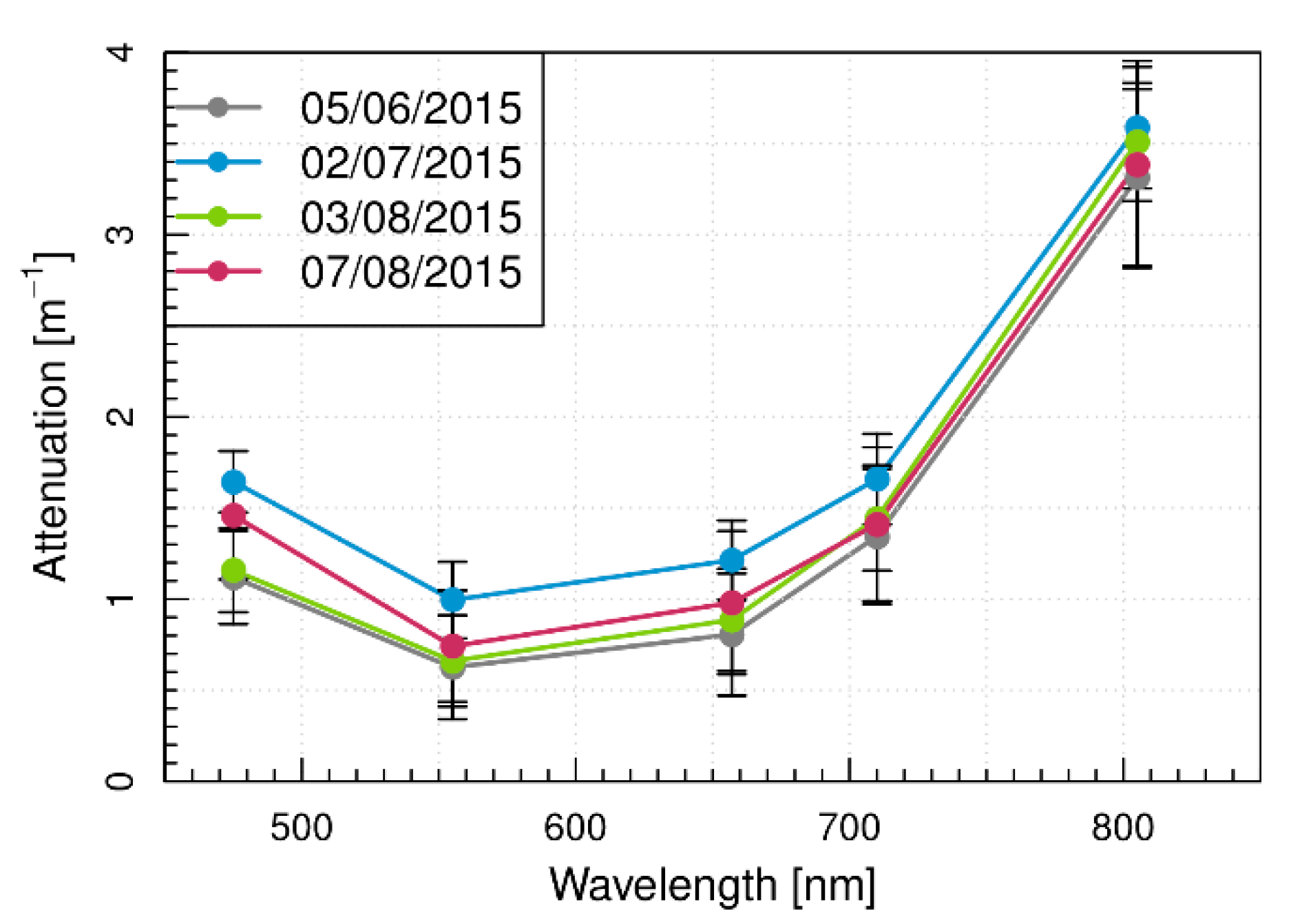
Median, 25% and 75% quartiles of were resampled to the RapidEye spectral response curves and used for the validation of ATCOR2 atmospheric correction. The vertical attenuation coefficient of , [m−1] was calculated using the equation by Maritorena [46] [Equation (3)].
(λ) and (λ) in Equation (3) were the median spectra of around 30 measurements. Retrieved spectra were resampled to the RapidEye spectral response curves and averaged from all measurement sites for each measurement day. Additional irradiance reflectance spectra ( [-]) of bare sediment and vegetation (Potamogeton pectinatus) were collected ex situ with an ASD LabSpec4515 (Analytical Spectral Devices Inc.; range: 350 nm to 2500 nm; interval: 1 nm). Following the method of Giardino et al. [27] SAV was harvested and its spectral response was then being measured at the beach (ex situ). Mean and standard deviations of single measurements were computed and resampled to RapidEye spectral response curves.
2.3. RapidEye Data and Processing
RapidEye Science Archive (RESA) provided multispectral L3A RapidEye data (included bands: blue 440–510 nm, green 520–590 nm, red 630–690 nm, red-edge 690–730 nm and near-infrared 760–880 nm) acquired at Lake Kummerow on 12 June, 1 July, 1 August and 7 August 2015. L3A products included a standard geometric correction resampled to a 5 × 5 m2 pixel size (coordinate system: WGS 1984, UTM Zone 33 N); units were at-sensor radiances [W m–2 nm−1]. Atmospheric correction (including atmospheric absorption and scattering, sensor and solar geometry) from at-sensor radiances to bottom of atmosphere irradiance reflectance [-] was conducted using ATCOR2 [29,47] for each date. ATCOR2 irradiance reflectance was converted to field measurement-comparable , followed a division by pi [48]. ATCOR2 automatically adapted visibility and corrected for adjacency effects with an adjacency range of 1 km. This effect was particularly strong at boundaries of surfaces with contrasting irradiance reflectance intensities, such as land and water above 700 nm wavelength. The aerosol model chosen was maritime mid-latitude summer, since north-easterly or north-western wind directions predominated during image acquisition. Thus, maritime aerosols from the Baltic Sea strongly influenced the study area. ATCOR2 estimated aerosol optical thickness at 550 nm (AOT 550 nm) on a per pixel basis applying the dense dark vegetation approach [49]. Moderate-resolution Imaging Spectroradiometer (MODIS) products served as a basis for evaluating the ATCOR2 results. Specifically, calculated AOT values were compared with MODIS AOT [50,51] acquired close to RapidEye image acquisition time. Specific settings of atmospheric correction and weather conditions close to image acquisition were summarized (Table 1).
To evaluate the performance of atmospheric correction, atmospherically corrected RapidEye data were also compared with in situ measured spectra. Arithmetic means and standard deviations were calculated from atmospherically corrected RapidEye data () based on a 5×5 pixel window surrounding the pixel which corresponded to the GPS coordinate of the respective measurement site. Accuracy indicators were calculated for bands 1 to 4, including root-mean-squared error (RMSE), Pearson’s correlation coefficient (r), and percentage bias (pbias) using the R package hydroGOF [52]. RMSE gives an indication of the absolute difference between in situ and atmospherically corrected spectra, r assesses accordance in shape, and pbias provides a relative statement.
Distinguishing water and land area was conducted by thresholding RapidEye near the infrared band (RapidEye band 5; central wavelength 805 nm). Pixels with values higher than 0.16 sr−1 were classified as land, masked and not further analysed. Water pixels were further processed by applying the deep water corrected Red Index () [53] [Equation (4)]. The value separates shallow water areas from optically deep water.
with representing remote sensing the reflectance value of each pixel in the red, and
representing red remote sensing reflectance over optically deep water.
depends on the water constituents and was empirically defined for Lake Kummerow with a threshold at 0.43. For this, water pixels with a higher than 0.43 were defined as shallow water and included in the further analysis.
Varying water constituent concentrations and water depths influence the signal received by sensors. To retrieve information about littoral bottom types, the influence of the water column at different water depths had to be considered. Absorption by water and its constituents reduce the availability of radiation with increasing depth, and the fraction of scattered radiation superimposes the radiation reflected by the lake bottom surface type. Depth-invariant indices () calculated from two spectral bands and are an option to reduce the influence of water constituents, and to investigate different littoral bottom types. To reduce the influence of the water column in satellite data, we applied the method of Lyzenga [35] considering that the attenuation coefficients and accounted for the present water constituent conditions in the water column and the absorption of the water column itself. Thus, the spectral features of the littoral bottom became visible. was linearized for each band using the natural logarithm of each spectral band [Equation (5)]. The logarithm was calculated for shallow water remote sensing reflectance [;] from which deep water remote sensing reflectance [] was subtracted. Lyzenga’s equation [Equation (5)] was applied to each RapidEye scene and to ex situ measurements of sediment and aquatic vegetation.
: RapidEye band ,
: RapidEye band , where ,
; : Diffuse attenuation coefficients of at band and ,
: Remote sensing reflectance at band and of each pixel,
: Deep-water remote sensing reflectance at band and .
2.4. Evaluation of SAV Mapping
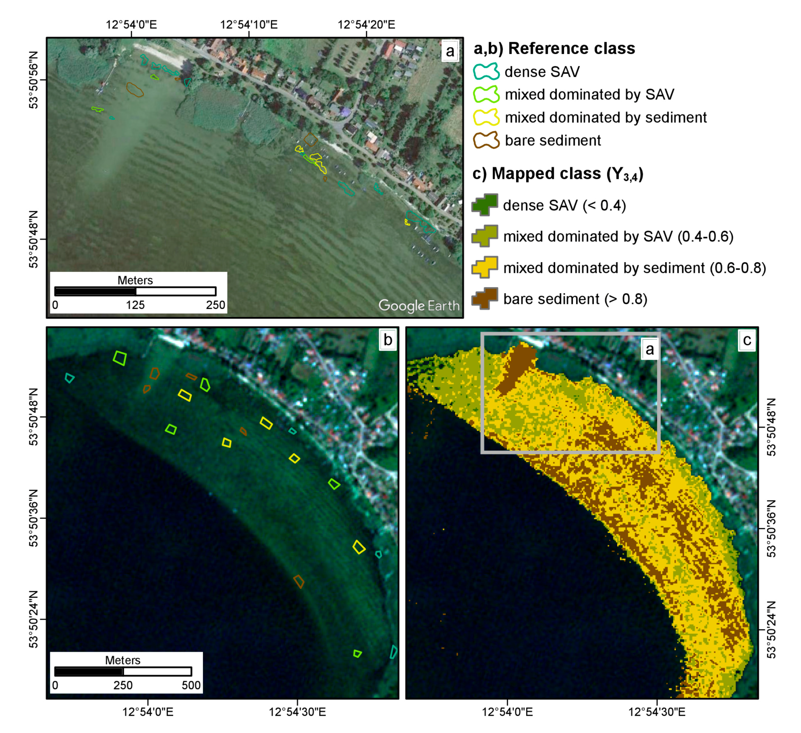
To obtain in situ data on macrophyte distribution at the northern end of the lake, we conducted lake substrate mappings in shallow water (<0.8 m water depth) close to the shoreline during the summer of 2015. These mappings served to evaluate the calculated index values, the size, position, and type of the lake bottom substrate. We mapped 21 easily accessible patches close to the shoreline with homogenous substrate or SAV coverage using a Trimble Juno SB GPS device [44]. Mapping homogeneous patches in situ at least three times larger than the pixel size as suggested by Dekker et al. [26] was limited to a small extent, particularly for SAV covered areas. Google Earth imagery (acquisition date: 9 August 2015) therefore served as a further evaluation basis. By visually comparing the mapped areas with patterns in Google Earth imagery, we could digitise larger patches (dense SAV coverage, mixed coverage SAV dominated, mixed coverage sediment dominated, pure sediment) better suited for a comparison with RapidEye results. We randomly chose five clearly identifiable patches per coverage class. The patches of dense SAV/pure sediment were chosen to be smaller (patch size ~500 m2) than patches of mixed classes (patch size ~800 m2) to avoid mixing. We calculated an error matrix as cross-tabulations between validation data and categorised depth-invariant index pixels. Cohen’s kappa and overall accuracy were calculated to assess the accuracy of the entire map as well as class specific accuracy measures (producer’s and user’s accuracy) [54,55].
3. Results
The spectral signatures of SAV and sediment revealed clear differences of irradiance reflectance for each wavelength region. For each acquisition date, several combinations of depth-invariant indices indicated a distinct discrimination between the two considered littoral bottom substrates. The results further demonstrated that Rapid Eye was able to map seasonal changes in SAV coverage.
3.1. Differentiation of Littoral Bottom Coverage
Mean for each measurement date, resampled to RapidEye, corresponded well in shape and intensity (Figure 2). Water constituents derived from in situ taken samples [suspended particulate material (SPM), Chl a, absorption by coloured dissolved organic matter (cDOM)] and Secchi depths varied for acquisition dates. Between 1 July and 7 August, Chl a concentration increased, while Secchi depth and SPM concentration decreased (Table 2).
Mean ex situ irradiance reflectance spectra of bare sediment and dense SAV were resampled to RapidEye bands (Figure 3a). The spectra clearly differed in intensity and shape. Calculating depth-invariant indices revealed a good discrimination between dense SAV and bare sediment for several combinations (, , , ) (Figure 3b). For each acquisition date, distinct thresholds for bare sediment and dense SAV were calculated. Depth-invariant indices and revealed a clear differentiation, but these band combinations were omitted due to the influence of cDOM. Even though the difference between dense SAV and the bare sediment of index was higher, index between RapidEye band 3 (657 nm) and band 4 (710 nm) was chosen for mapping SAV coverage. The influence of the atmosphere in the adjacent red (band 3) and red edge (band 4) region of the spectra was less than between green (band 2) and red edge bands. In particular, covered a characteristic vegetation feature, the red edge, i.e., the passage where reflectance strongly increases between visible red and near infrared wavelengths. Due to strong attenuation of water in near-infrared wavelengths (Figure 2) this feature is normally superimposed by water absorption [23]. To minimize the influence of water absorption, was included in the index calculation. Thus, the influence of the exponential decline of radiation with increasing water depth can be omitted [56]. Depth-invariant index revealed clearly different index values for the two substrate types. Based on ex-situ measured spectra, values around 0 indicated dense coverage with SAV and values above 0.8 indicated bare sediment (Figure 3b). Values in between these thresholds referred to pixels with a mixed coverage of SAV and sediment.
3.2. Seasonal Changes of Littoral Bottom Coverage
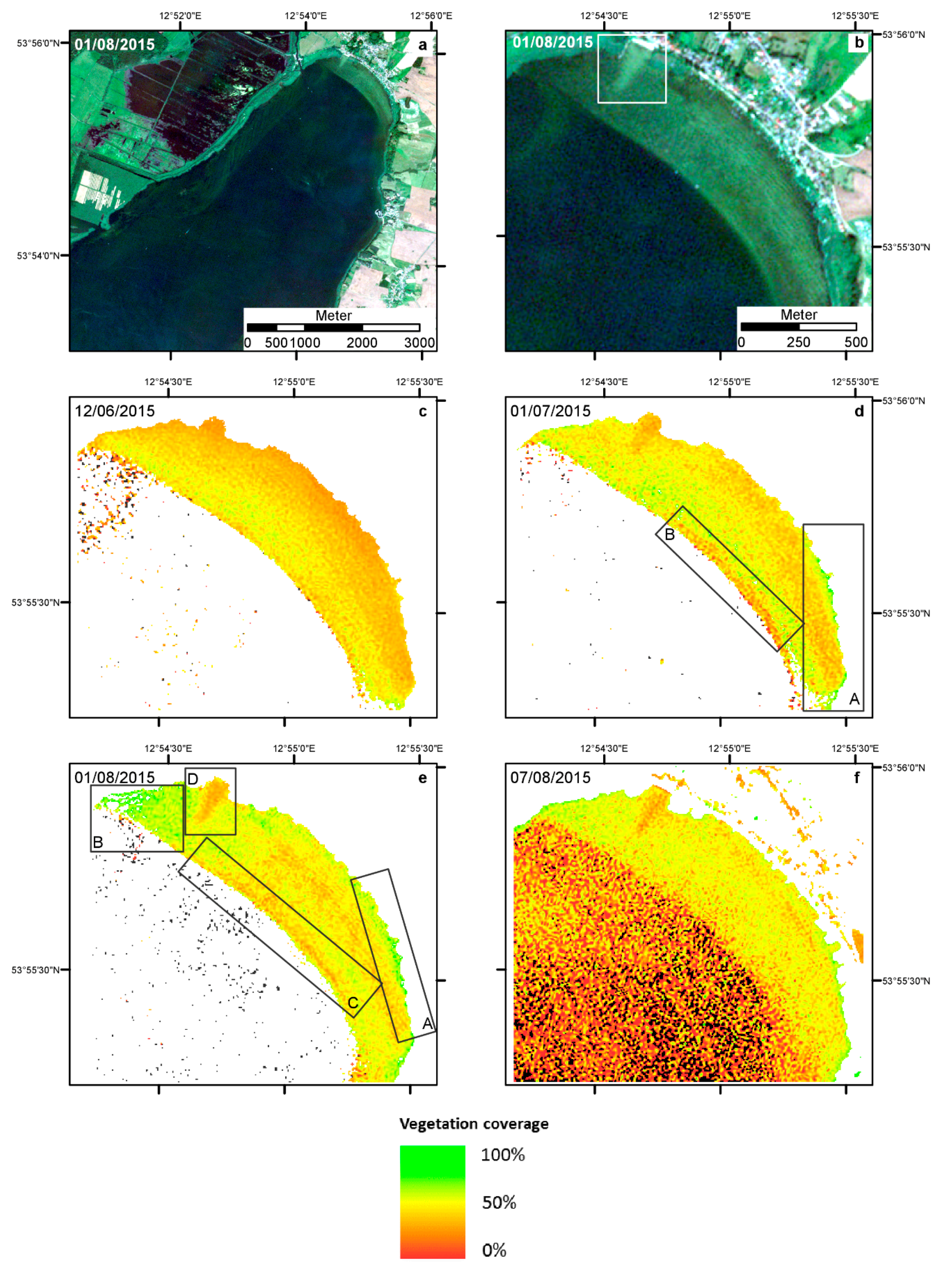
Due to its extensive shallow water area, the northern part (Figure 4b) of Lake Kummerow seemed most suitable for analysing bottom substrate (Figure 4a). Different bottom colours (bright and dark) and structures (e.g., bright triangle, Figure 4b, white box) were visible in the true-colour composite and indicated varying bottom coverage. The depth-invariant index (Figure 4c–f) illustrated changes in SAV coverage at the northern littoral. The SAV coverage was scaled between 0% (equivalent to bare sediment, red) and 100% (equivalent to complete macrophyte cover, green). Invalid pixels (black) were those upon which the depth-invariant index could not be executed.
In the RapidEye data set from 5th June (Figure 4c), most parts of the shallow area were classified as sediment. A few areas displayed mixed pixels with values between the thresholds of bare sediment and dense SAV. First, distinct SAV patches appeared in the data set from 1st July (Figure 4d) close to the shoreline (Figure 4, box A). A small strip of bare sediment was present at the transition to the deep water region (Figure 4d, box B). On 1st August, SAV patches spread and formed large SAV-covered areas (Figure 4e, box A and B); most of the former bare sediment areas changed their index value indicating mixed pixels now. Patches predominated by sediment, such as the linear structure near deep water (Figure 4d, box C), expanded as well. In the northern part, a triangular sediment structure (Figure 4d, box D) became apparent. On 7 August (Figure 4f), a separation between deep and shallow water failed. The index classified most deep water pixels as sediment. The actual shallow water appeared as a heterogeneously mixed area except for the sediment triangle in the north and dense SAV patches near the shoreline.
3.3. Evaluation of SAV Mapping
To evaluate the depth-invariant index classification, local scale in situ mappings covering diverse structures of littoral bottom and Google Earth imagery (acquisition date: 9 August) served as a basis (Figure 5a). Mapping during summer months revealed that SAV started to grow sparsely at the beginning of June. In accordance with the official WFD monitoring (conducted in 2013, Figure 1a), Potamogeton pectinatus was the predominating patch-forming species. Patches mapped as pure sediment corresponded to bright areas visible in the Google Earth image. Patches mapped as pure SAV coverage (Potamogeton pectinatus) mainly matched with dark areas. In particular, at small patches, problems associated with GPS positional accuracy became apparent. Mixed coverages with dominating sediment showed patterns similar to ripple marks, i.e., an approximately 10 m wide sediment strip followed an approximately 5 m wide SAV strip (Figure 5a). The validation areas were digitised referring to the following categories: dense SAV, mixed coverage dominated by SAV, mixed coverage dominated by sediment and pure sediment (Figure 5b). Figure 5c displays the categorized depth-invariant index of 1 August. We determined thresholds between classes based on ex situ measured spectra and in situ mapped patches similar to Brooks et al. [38]. Table 3 lists the tabulated error matrix and accuracy measures. SAV mapping in the northern part of the lake revealed an overall accuracy of 72.2% and a kappa coefficient of 0.61.
3.4. Atmospheric Correction
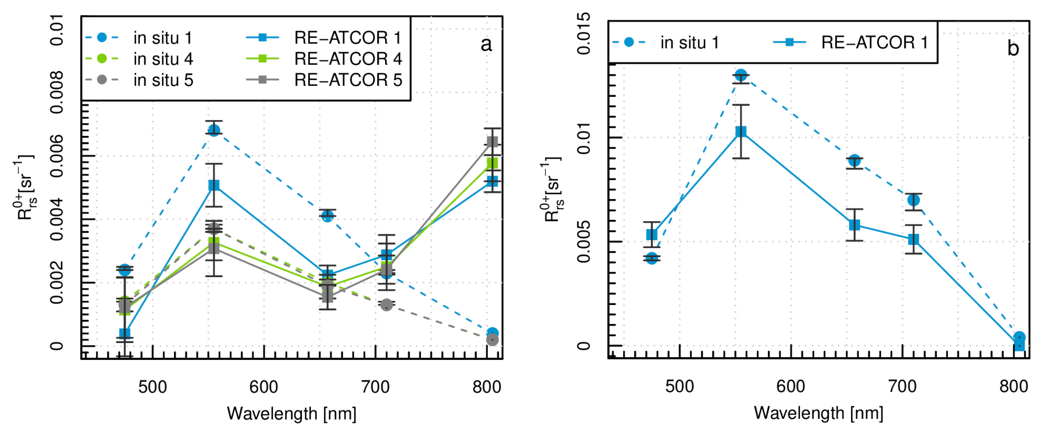
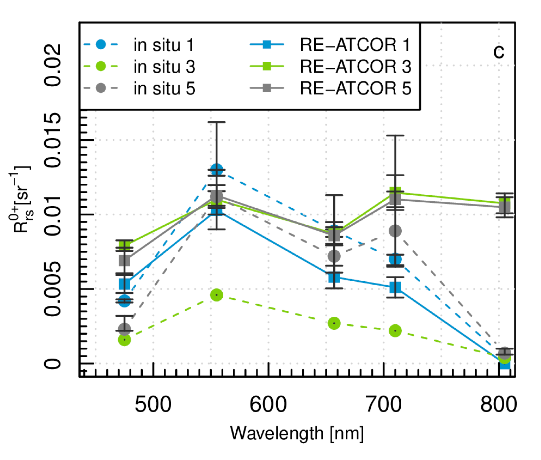
Between the three evaluation dates, comparing in situ and RapidEye spectra revealed differences in both shape and intensity (Figure 6). Largest discrepancies occurred in band 5, which consistently showed higher RapidEye than in-situ values. For most measurement sites, in-situ and RapidEye spectra correlated reasonably in shape between band 1 and 4 (r > 0.6). ATCOR2 overestimated absolute values except for 1 August and 2 July (measurement site 1). On 2 July, calculated RMSE and percentage bias were low for sites 3–5 on this date, indicating a good correspondence in intensities between atmospherically corrected and in situ measured data (Table 4). On 1 August, in situ measurements were available from one site only, over bare sediment in optically shallow water (around 1.5 m water depth). On this day, atmospherically corrected RapidEye spectra showed lower values compared to the in situ data, but corresponded well in shape (Figure 6b). On 7 August, ATCOR2 corrected RapidEye spectra were significantly higher than in situ data and showed the highest pbias and RMSE (Table 4). Evaluation of this date indicated an erroneous atmospheric correction; only measurement site 5, located close to shallow water, showed acceptable correspondence in shape and intensity (Figure 6c). The second indicator of atmospheric performance was ATCOR2-calculated AOT (550 nm) in comparison to the MODIS AOT product. During the investigation period, AOT (550 nm) was highest on 7 August; lowest values occurred on 1 August. AOT (550 nm) values from MODIS products showed the same tendency between acquisition dates (Table 5). Retrieved values slightly differed between MODIS product and ATCOR2-RapidEye.
4. Discussion
The present study tests the applicability of RapidEye satellite data with its high spatial resolution and its high revisiting frequency to map SAV in shallow areas of eutrophic freshwater lakes. The identification of SAV patches and the monitoring of the phenologic development of SAV was successful, even though the atmospheric correction of RapidEye satellite data was conducted using ATCOR2.
4.1. Differentiation and Seasonal Changes of Littoral Bottom Coverage
The results indicated that multi-seasonal RapidEye data are suitable for monitoring changes in littoral bottom coverage as previously proposed by several authors [15,19,27,38,39]. Our approach follows several studies which successfully applied depth-invariant indices to discriminate between SAV and sediment [19,38,39]. In our study, the depth-invariant index , combining RapidEye band 3 and 4, performed well in mapping the general trend of SAV expansion within the observation period (Figure 4c–f). In the shallow water zone, SAV favour calm regions near the shoreline resulting in dense patches while sediment dominates in areas with high disturbance due to wind [57], waves, and human activities.
High wind and wave activities influenced the expansion of macrophytes at the beginning of the vegetation period. On 12th June, sediment covered most of the lake bottom. Vegetation was sparsely distributed; field observation confirmed the growth of SAV at the beginning of June. Moreover, detritus, plant residuals, epiphytes, or sparsely growing SAV influenced the spectral signal, resulting in an index value of mixed coverage [6,15,21,22,23].
From 1st July to 1st August, the SAV covered area increased, especially at calm regions near the shoreline (Figure 4d, box A; Figure 4e, box A and B), where the spectral signature showed a vegetation dominated signal. Sediment dominated highly disturbed areas such as the beach (Figure 4e, box D). The linear sediment zone near the deep water border (Figure 4d, box B; Figure 4e, box C) may be attributed to wave pounding.
Limitations of the index method appeared to be related mainly to the concentration of optically active water constituents and the measurement. Within one week (1st August–7th August), SPM and Chl-a concentrations in the water column increased strongly; the water transparency decreased accordingly (Table 2). Low Secchi depths indicated high light attenuation in the water column. An algal bloom, as imaged on 7th August 2015 (Figure 4f and [58]) hampered a successful discrimination between deep and shallow water; failed to separate shallow and deep water. Therefore, the depth-invariant index was calculated for the entire water body. During the algal bloom, surface-floating algae increased RapidEye values over the entire lake. In situ measurements (Figure 2), however, remained at a similar intensity. Water samples and measurement setup may have caused this discrepancy: water samples were collected close to the water surface. Floating algae therefore may have influenced the water samples and satellite signals. For measurements the sensors were installed on a floating device which may have partially removed the algae carpet. The resulting values would therefore have failed to represent actual water conditions. Non-representative values resulted in high RapidEye values, which in turn indicated high sediment coverage (Figure 4f). Consequently, extreme events such as algal blooms have to be considered, and data collected during such events have to be carefully checked for such a bias.
4.2. Evaluation of SAV Mapping
Validating SAV distribution and coverage is a challenging task. The littoral bottom coverage is often difficult to access. In situ observations therefore are conducted on selective transects by divers or from boat and therefore cover only small areas hardly transferable to the satellite level. GPS inaccuracies and a system that is in motion introduce positional errors to the observation. Several studies therefore evaluate mappings qualitatively [16,19,27,59]. Studies which determined discrete classes (e.g., less dense SAV, bare substrate, submerged, floating vegetation) collected field data by boat or ancillary maps to tabulate error matrices and associated accuracy measures [38,39,60,61,62]. Dekker et al. [26] recommend a minimum patch size of at least three times the pixel size covering homogenous coverage. The limited overview during in situ mapping, however, hampers identifying homogenous patches of at least 75 m2. We therefore followed an approach which recently proved valuable in remote sensing studies on land use/cover [63,64,65], i.e., a comparison with Google Earth imagery. We verified the visual interpretation of Google Earth imagery with in situ mapped patches. The spatial resolution of Google Earth images is higher than RapidEye, the information (e.g., species, bottom type) is less detailed than in situ mappings, but grants a spatial overview. Upscaling the extent of in situ data by means of very high spatial resolution aerial or Google Earth imagery may help to overcome the limitation associated with comparing limited in situ and satellite data.
Other studies conducting accuracy assessments [31,38,39,60,61,62] show kappa coefficients ranging between 0.57 and 0.92. The result of our study is at the lower end of the scale (kappa = 0.61). Producer’s and user’s accuracies highlight varying performance of the different classes. Bare sediment is easy to detect and performs best (Table 3). Reference patches of dense SAV often include land-masked pixels; dense SAV that grew up to the water surface developing surface floating leaves may have led to erroneous land masking. Mixed coverage dominated by SAV partially mixes up with mixed coverage dominated by sediment. A clear differentiation between both classes is difficult for both Google Earth digitisation and Y3,4. The spatial resolution of RapidEye misses the structures similar to ripple waves, which are clearly apparent in the Google Earth imagery (Figure 5).
Bridging the gap between in situ and satellite mapping via Google Earth is only possible when near-term imagery is available as for the RapidEye data set from 1 August 2015. The evaluation of at least one data set offers a first impression of the applied method’s accuracy. To evaluate growth patterns, mapping of pilot sites is necessary close to satellite acquisitions. Assessing the plausibility of growth patterns or recurring uniform patches (e.g., triangular structure of sediment) may be a further option for a qualitative evaluation.
4.3. Atmospheric Correction
To adjust and evaluate the atmospheric correction process of the RapidEye data with ATCOR2, two different approaches were employed, i.e., the comparison with in situ submersible spectroradiometer data and the MODIS products as delivered by the NASA standard processing chain. Both methods are prone to errors and contain uncertainties; nevertheless, they allowed for a complementary evaluation of results.
Simultaneously taken in situ and remote sensing data sets are considered the most reliable proof for a successful atmospheric correction. The empirical line approach [66], for instance, is based on this assumption. The policy of the RapidEye company (later BlackBridge, now Planet Labs) gave priority to commercial orders and, prohibited a precise acquisition planning and field data collection. For this reason, evaluation of atmospheric correction was only possible based on a relatively small in situ data set. Simultaneous in situ and satellite measurements were available solely on 1st and 7th August; on 1 July a time gap of one day existed.
In situ data included measurements of upwelling radiance below water surface, which are then extrapolated to above water surface reflectance (. Water surface effects, such as sun and sky glint, therefore remained unaddressed in the resulting in situ spectra. Contrarily, two overlaying phenomena probably contaminated the ATCOR2 atmospherically corrected spectra: sky/sun glint and insufficiently addressable adjacency effects. The latter, in particular, affects bands in wavelength regions above 700 nm [67,68,69]. The spectral signature of water is influenced by additional radiation from neighbouring, vegetated land surfaces with much higher reflectance in these wavelengths. This effect may contribute to water pixels up to 5 km away from the shoreline [67,68], Figure 6a,c, i.e., bands 3–5). On 1st August, only one in situ data set existed; in this case, however, an almost perfect match in shape indicated a good performance of atmospheric correction at least at this site in optically shallow water.
During the algal bloom (7 August), below-water surface in situ radiometric measurements may not have captured the actual conditions at the water surface; surface cum algae, however, seem to dominate the RapidEye signal leading to be observed differences between in situ and RapidEye spectra.
Due to the limited match with in situ measurements, MODIS AOT products served as a second indicator for evaluating the atmospheric correction. Overall, ATCOR2 AOT of RapidEye data was slightly lower compared to MODIS (pbias = − 13.5%) but are highly comparable (r = 0.94). Low AOT (550 nm) values (Table 4) indicated clear atmospheric conditions. On these days, RapidEye data matched fairly well with in situ spectra. On 7 August (Figure 6c), AOT values at 550 nm were relatively high, i.e., 0.301 for corrected ATCOR2-RapidEye data and 0.390 for the MODIS product; both values indicated a hazy, dense atmosphere and a consequently difficult correction of atmospheric effects (e.g., absorption and scattering).
The differences between in situ and atmospherically corrected spectra reflected the challenges for this correction procedure, which were further aggravated by an algae bloom. The successful differentiation of optically deep and shallow water and subsequent delineation of macrophytes/sediment coverage, however, depended on the performance of atmospheric correction. Further improvements of strategies and sensor-generic software packages for freshwater lake atmospheric correction, therefore, are necessary when envisaging a systematic SAV monitoring. Until such algorithms are available comparisons with in situ measurements help to consider issues related to atmospheric correction when interpreting SAV mapping.
5. Conclusions
This study used four ATCOR2 corrected RapidEye data sets (June to August 2015) to map SAV in the shallow water areas of the eutrophic Lake Kummerow (North-Eastern Germany). Radiometric field measurements supported parameterising a depth-invariant index, which reduced the influence of the overlaying water on the bottom signal. The index enabled mapping the growth and spatial distribution of SAV. Growth patterns showed the expected spatio-temporal development of SAV. The index, however, failed during a surface scum forming algal bloom. Gathering reference data for quantitative evaluations is a challenge; comparisons with field mappings and Google Earth imagery revealed realistic and sufficient accuracies (kappa coefficient = 0.61, overall accuracy = 72.2%) in comparison to other studies. The spectral resolution of RapidEye may be insufficient to gain information on species level especially for mono-temporal data investigations. Implementing ecologic and physiological characteristics, such as phenologic or structural changes of SAV and information on species-specific canopy height, may help to identify species. In view of global warming, multi-year time-series may obtain information about trends in SAV coverage. Recent data may help to detect areas, which undergo changes; targeted diver mappings may reveal specific details. Thus, satellite systems with high spatial resolution and revisiting frequency offer the potential to support in situ macrophyte surveys as conducted within the WFD.
Acknowledgments
This research was founded by the Federal Ministry for Economic Affairs and Energy (BMWi) under the grant numbers 50EE1336 and 50EE1340 within the project LAKESAT. We thank Planet Labs for providing us with RapidEye satellite data within RapidEye Research Archive (RESA) project No. 194. Thanks to all colleagues from the Limnological Research Station Iffeldorf and from CAU Kiel for assistance in fieldwork and laboratory analyses. We thank three anonymous reviewers for their effort and helpful comments.
Author Contributions
Christine Fritz, Katja Dörnhöfer, Thomas Schneider, Jürgen Geist and Natascha Oppelt conceived and designed the study. Christine Fritz wrote the majority of the paper and analysed image data. Katja Dörnhöfer conducted atmospheric correction and SAV evaluation. All authors contributed equally in reviewing and finalizing the manuscript.
Conflicts of Interest
The authors declare no conflict of interest.
References
- Melzer, A. Aquatic macrophytes as tools for lake management. Hydrobiologia 1999, 395, 181–190. [Google Scholar] [CrossRef]
- Penning, W.E.; Dudley, B.; Mjelde, M.; Hellsten, S.; Hanganu, J.; Kolada, A.; van den Berg, M.; Poikane, S.; Phillips, G.; Willby, N.; et al. Using aquatic macrophyte community indices to define the ecological status of European lakes. Aquat. Ecol. 2008, 42, 253–264. [Google Scholar] [CrossRef]
- Skubinna, J.P.; Coon, T.G.; Batterson, T.R. Increased abundance and depth of submersed macrophytes in response to decreased turbidity in Saginaw Bay, Lake Huron. J. Great Lakes Res. 1995, 21, 476–488. [Google Scholar] [CrossRef]
- Søndergaard, M.; Johansson, L.S.; Lauridsen, T.L.; Jørgensen, T.B.; Liboriussen, L.; Jeppesen, E. Submerged macrophytes as indicators of the ecological quality of lakes. Freshw. Biol. 2010, 55, 893–908. [Google Scholar] [CrossRef]
- Poikane, S.; Birk, S.; Böhmer, J.; Carvalho, L.; de Hoyos, C.; Gassner, H.; Hellsten, S.; Kelly, M.; Lyche Solheim, A.; Olin, M.; et al. A hitchhiker’s guide to European lake ecological assessment and intercalibration. Ecol. Indic. 2015, 52, 533–544. [Google Scholar] [CrossRef]
- Silva, T.S.F.; Costa, M.P.F.; Melack, J.M.; Novo, E.M.L.M. Remote sensing of aquatic vegetation: Theory and applications. Environ. Monit. Assess. 2008, 140, 131–145. [Google Scholar] [CrossRef] [PubMed]
- Short, F.T.; Neckles, H.A. The effects of global climate change on seagrasses. Aquat. Bot. 1999, 63, 169–196. [Google Scholar] [CrossRef]
- Rooney, N.; Kalff, J. Inter-annual variation in submerged macrophyte community biomass and distribution: The influence of temperature and lake morphometry. Aquat. Bot. 2000, 68, 321–335. [Google Scholar] [CrossRef]
- European Commission. The water framework directive (directive 2000/60/EC of the European Parliament and of the Council of 23 October 2000 establishing a framework for Community action in the field of water policy). Off. J. Eur. Commun. Bruss. Belg. 2000, 22, 1–72. [Google Scholar]
- Palmer, S.C.J.; Kutser, T.; Hunter, P.D. Remote sensing of inland waters: Challenges, progress and future directions. Remote Sens. Environ. 2015, 157, 1–8. [Google Scholar] [CrossRef]
- Dörnhöfer, K.; Oppelt, N. Remote sensing for lake research and monitoring-recent advances. Ecol. Indic. 2016, 64, 105–122. [Google Scholar] [CrossRef]
- George, D.G. The airborne remote sensing of phytoplankton chlorophyll in the lakes and tarns of the English Lake District. Int. J. Remote Sens. 1997, 18, 1961–1975. [Google Scholar] [CrossRef]
- Dekker, A.G.; Vos, R.J.; Peters, S.W.M. Analytical algorithms for lake water TSM estimation for retrospective analyses of TM and SPOT sensor data. Int. J. Remote Sens. 2002, 23, 15–35. [Google Scholar] [CrossRef]
- Malthus, T.J.; George, D.G. Airborne remote sensing of macrophytes in Cefni Reservoir, Anglesey, UK. Aquat. Bot. 1997, 58, 317–332. [Google Scholar] [CrossRef]
- Wolf, P.; Rößler, S.; Schneider, T.; Melzer, A. Collecting in situ remote sensing reflectances of submersed macrophytes to build up a spectral library for lake monitoring. Eur. J. Remote Sens. 2013, 46, 401–416. [Google Scholar] [CrossRef]
- Giardino, C.; Bartoli, M.; Candiani, G.; Bresciani, M.; Pellegrini, L. Recent changes in macrophyte colonisation patterns: An imaging spectrometry-based evaluation of southern Lake Garda (northern Italy). J. Appl. Remote Sens. 2007, 1, 011509–011517. [Google Scholar]
- Yuan, L.; Zhang, L.-Q. Mapping large-scale distribution of submerged aquatic vegetation coverage using remote sensing. Ecol. Inform. 2008, 3, 245–251. [Google Scholar] [CrossRef]
- Pinnel, N.; Heege, T.; Zimmermann, S. Spectral discrimination of submerged macrophytes in lakes using hyperspectral remote sensing data. SPIE Proc. Ocean Optics XVII 2004, 1, 1–16. [Google Scholar]
- Roessler, S.; Wolf, P.; Schneider, T.; Melzer, A. Multispectral remote sensing of invasive aquatic plants using RapidEye. In Earth Observation of Global Changes (EOGC); Krisp, J.M., Meng, L., Pail, R., Stilla, U., Eds.; Springer: Berlin/Heidelberg, Germany, 2013; pp. 109–123. [Google Scholar]
- Malthus, T.J.; Karpouzli, E. Integrating field and high spatial resolution satellite-based methods for monitoring shallow submersed aquatic habitats in the Sound of Eriskay, Scotland, UK. Int. J. Remote Sens. 2003, 24, 2585–2593. [Google Scholar] [CrossRef]
- Williams, D.J.; Rybicki, N.B.; Lombana, A.V.; O’Brien, T.M.; Gomez, R.B. Preliminary investigation of submerged aquatic vegetation mapping using hyperspectral remote sensing. Environ. Monit. Assess. 2003, 81, 383–392. [Google Scholar] [CrossRef]
- Fyfe, S. Spatial and temporal variation in spectral reflectance: Are seagrass species spectrally distinct? Limnol. Oceanogr. 2003, 48, 464–479. [Google Scholar] [CrossRef]
- Armstrong, R.A. Remote sensing of submerged vegetation canopies for biomass estimation. Int. J. Remote Sens. 1993, 14, 621–627. [Google Scholar] [CrossRef]
- Gausman, H.W. Evaluation of factors causing reflectance differences between sun and shade leaves. Remote Sens. Environ. 1984, 15, 177–181. [Google Scholar] [CrossRef]
- Gitelson, A.A.; Zur, Y.; Chivkunova, O.B.; Merzlyak, M.N. Assessing carotenoid content in plant leaves with reflectance spectroscopy. Photochem. Photobiol. 2002, 75, 272–281. [Google Scholar] [CrossRef]
- Dekker, A.G.; Phinn, S.R.; Anstee, J.; Bissett, P.; Brando, V.E.; Casey, B.; Fearns, P.; Hedley, J.; Klonowski, W.; Lee, Z.P. Intercomparison of shallow water bathymetry, hydro-optics, and benthos mapping techniques in Australian and Caribbean coastal environments. Limnol. Oceanogr. Methods 2011, 9, 396–425. [Google Scholar] [CrossRef]
- Giardino, C.; Bresciani, M.; Valentini, E.; Gasperini, L.; Bolpagni, R.; Brando, V.E. Airborne hyperspectral data to assess suspended particulate matter and aquatic vegetation in a shallow and turbid lake. Remote Sens. Environ. 2015, 157, 48–57. [Google Scholar] [CrossRef]
- Heege, T.; Bogner, A.; Pinnel, N. Mapping of Submerged Aquatic Vegetation with a Physically Based Processing Chain; Kramer, E., Ed.; SPIE-The International Society for Optical Engineering: Barcelona, Spain, 2003; pp. 43–50. [Google Scholar]
- Richter, R.; Schläpfer, D. Atmospheric/Topographic Correction for Satellite Imagery: Atcor-2/3 User Guide, Version 9.1.0, dlr/rese, wessling, dlr-ib 565-01/16. October 2016. Available online: http://www.Rese-apps.Com/pdf/atcor3_manual.pdf (accessed on 30 November 2016).
- Gege, P. A case study at starnberger see for hyperspectral bathymetry mapping using inverse modeling. In Proceedings of the WHISPERS 2014, Lausanne, Switzerland, 25–27 July 2014; pp. 1–4. [Google Scholar]
- Villa, P.; Bresciani, M.; Bolpagni, R.; Pinardi, M.; Giardino, C. A rule-based approach for mapping macrophyte communities using multi-temporal aquatic vegetation indices. Remote Sens. Environ. 2015, 171, 218–233. [Google Scholar] [CrossRef]
- Giardino, C.; Candiani, G.; Bresciani, M.; Lee, Z.; Gagliano, S.; Pepe, M. Bomber: A tool for estimating water quality and bottom properties from remote sensing images. Comput. Geosci. 2012, 45, 313–318. [Google Scholar] [CrossRef]
- Lyzenga, D.R. Passive remote sensing techniques for mapping water depth and bottom features. Appl. Opt. 1978, 17, 379–383. [Google Scholar] [CrossRef] [PubMed]
- Gege, P. WASI-2D: A software tool for regionally optimized analysis of imaging spectrometer data from deep and shallow waters. Comput. Geosci. 2013, 62, 208–215. [Google Scholar] [CrossRef]
- Lyzenga, D.R. Remote sensing of bottom reflectance and water attenuation parameters in shallow water using aircraft and Landsat data. Int. J. Remote Sens. 1981, 2, 71–82. [Google Scholar] [CrossRef]
- Manessa, M.D.M.; Kanno, A.; Sekine, M.; Ampou, E.E.; Widagti, N.; As-syakur, A.R. Shallow-water benthic identification using multispectral satellite imagery: Investigation on the effects of improving noise correction method and spectral cover. Rem. Sens. 2014, 6, 4454–4472. [Google Scholar] [CrossRef]
- Ciraolo, G.; Cox, E.; La Loggia, G.; Maltese, A. The classification of submerged vegetation using hyperspectral MIVIS data. Ann. Geophys. 2006, 49, 287–294. [Google Scholar]
- Brooks, C.; Grimm, A.; Shuchman, R.; Sayers, M.; Jessee, N. A satellite-based multi-temporal assessment of the extent of nuisance Cladophora and related submerged aquatic vegetation for the Laurentian Great Lakes. Remote Sens. Environ. 2015, 157, 58–71. [Google Scholar] [CrossRef]
- Shuchman, R.A.; Sayers, M.J.; Brooks, C.N. Mapping and monitoring the extent of submerged aquatic vegetation in the Laurentian Great Lakes with multi-scale satellite remote sensing. J. Great Lakes Res. 2013, 39, 78–89. [Google Scholar] [CrossRef]
- Wöbbecke, K.; Klett, G.; Rechenberg, B. Wasserbeschaffenheit der Wichtigsten seen in der Bundesrepublik Deutschland: Datensammlung 1981–2000; Umweltbundesamt: Dessau-Roßlau, Germany, 2003. [Google Scholar]
- LU-MV. Investigation of Macrophytes in Selected Lakes Mecklenburg-Western Pomerania in the Year 2013 (Data Set). Lake Kummerow (200010). MLUV-MV 2015. Data Set Request at MLUV-MV. Available online: http://www.regierung-mv.de/Landesregierung/lm/Umwelt/Wasser/ (accessed on 11 July 2017).
- Schaumburg, J.; Schranz, C.; Stelzer, D. Bewertung von Seen mit Makrophyten & Phytobenthos gemäß EG-WRRL–Anpassung des Verfahrens für Natürliche und Künstliche Gewässer sowie Unterstützung der Interkalibrierung; Bayerisches Landesamt für Umwelt: Augsburg/Wielenbach, Germany, 2011. [Google Scholar]
- TriOS. Ramses Radiometer. Available online: http://www.Trios.De/en/products/sensors/ramses.Html (accessed on 29 November 2016).
- Trimble. Datasheet. Trimble Juno SD Handheld GPS Device. Available online: http://trl.Trimble.Com/docushare/dsweb/get/document-504948/022501-244b_juno%20sd_ds_0712_mgis_hr_nc.Pdf (accessed on 30 November 2016).
- Mobley, C.D. Estimation of the remote-sensing reflectance from above-surface measurements. Appl. Opt. 1999, 38, 7442–7455. [Google Scholar] [CrossRef] [PubMed]
- Maritorena, S. Remote sensing of the water attenuation in coral reefs: A case study in French Polynesia. Int. J. Remote Sens. 1996, 17, 155–166. [Google Scholar] [CrossRef]
- Richter, R. Correction of atmospheric and topographic effects for high spatial resolution satellite imagery. Int. J. Remote Sens. 1997, 18, 1099–1111. [Google Scholar] [CrossRef]
- Mobley, C.D.; Boss, E.; Roesler, C. Ocean Optics Web Book. 2015. Available online: http://www.oceanopticsbook.info/ (accessed on 10 July 2017).
- Kaufman, Y.; Tanré, D.; Gordon, H.; Nakajima, T.; Lenoble, J.; Frouin, R.; Grassl, H.; Herman, B.; King, M.; Teillet, P. Passive remote sensing of tropospheric aerosol and atmospheric correction for the aerosol effect. J. Geophysis. Res-Atmos. 1997, 102, 16815–16830. [Google Scholar] [CrossRef]
- Levy, R.; Hsu, C. MODIS Atmosphere L2 Aerosol Product (MYD04_L2). NASA MODIS Adaptive Processing System, Goddard Space Flight Center, USA. 2015a. Available online: http://dx.doi.org/10.5067/MODIS/MYD04_L2.006 (accessed on 10 July 2017).
- Levy, R.; Hsu, C. MODIS Atmosphere L2 Aerosol Product (MOD04_L2). NASA MODIS Adaptive Processing System, Goddard Space Flight Center, USA. 2015b. Available online: http://dx.doi.org/10.5067/MODIS/MOD04_L2.006 (accessed on 10 July 2017).
- Zambrano-Bigiarini, M. Hydrogof: Goodness-of-fit Functions for Comparison of Simulated and Observed Hydrological: R Package Version 0.3-8. Available online: https://cran.r-project.org/web/packages/hydroGOF/index.html (accessed on 10 July 2017).
- Spitzer, D.; Dirks, R.W.J. Bottom influence on the reflectance of the sea. Int. J. Remote Sens. 1987, 8, 279–308. [Google Scholar] [CrossRef]
- Foody, G.M. Status of land cover classification accuracy assessment. Remote Sens. Environ. 2002, 80, 185–201. [Google Scholar] [CrossRef]
- Congalton, R.G. A review of assessing the accuracy of classifications of remotely sensed data. Remote Sens. Environ. 1991, 37, 35–46. [Google Scholar] [CrossRef]
- Kirk, J.T. Light and Photosynthesis in Aquatic Ecosystems; Cambridge University Press: Cambridge, UK, 1994. [Google Scholar]
- Koch, E.W. Beyond light: Physical, geological, and geochemical parameters as possible submersed aquatic vegetation habitat requirements. Estuaries 2001, 24, 1–17. [Google Scholar] [CrossRef]
- Dörnhöfer, K.; Klinger, P.; Heege, T.; Oppelt, N. Multi-sensor satellite and in situ monitoring of phytoplankton development in a eutrophic-mesotrophic lake. Sci. Total Environ. In review.
- Heblinski, J.; Schmieder, K.; Heege, T.; Agyemang, T.K.; Sayadyan, H.; Vardanyan, L. High-resolution satellite remote sensing of littoral vegetation of Lake Sevan (Armenia) as a basis for monitoring and assessment. Hydrobiologia 2011, 661, 97–111. [Google Scholar] [CrossRef]
- Hunter, P.D.; Gilvear, D.J.; Tyler, A.N.; Willby, N.J.; Kelly, A. Mapping macrophytic vegetation in shallow lakes using the Compact Airborne Spectrographic Imager (CASI). Aquat. Conserv. Mar. Freshw. Ecosyst. 2010, 20, 717–727. [Google Scholar] [CrossRef]
- Dogan, O.K.; Akyurek, Z.; Beklioglu, M. Identification and mapping of submerged plants in a shallow lake using quickbird satellite data. J. Environ. Manag. 2009, 90, 2138–2143. [Google Scholar] [CrossRef] [PubMed]
- Bolpagni, R.; Bresciani, M.; Laini, A.; Pinardi, M.; Matta, E.; Ampe, E.M.; Giardino, C.; Viaroli, P.; Bartoli, M. Remote sensing of phytoplankton-macrophyte coexistence in shallow hypereutrophic fluvial lakes. Hydrobiologia 2014, 737, 67–76. [Google Scholar] [CrossRef]
- Wang, P.; Huang, C.; Brown de Colstoun, E.C. Mapping 2000–2010 impervious surface change in India using global land survey landsat data. Remote Sens. 2017, 9, 366. [Google Scholar] [CrossRef]
- Manakos, I.; Karakizi, C.; Gkinis, I.; Karantzalos, K. Validation and inter-comparison of spaceborne derived global and continental land cover products for the Mediterranean region: The case of Thessaly. Land 2017, 6, 34. [Google Scholar] [CrossRef]
- Bey, A.; Sánchez-Paus Díaz, A.; Maniatis, D.; Marchi, G.; Mollicone, D.; Ricci, S.; Bastin, J.-F.; Moore, R.; Federici, S.; Rezende, M. Collect earth: Land use and land cover assessment through augmented visual interpretation. Remote Sens. 2016, 8, 807. [Google Scholar] [CrossRef]
- Smith, G.M.; Milton, E.J. The use of the empirical line method to calibrate remotely sensed data to reflectance. Int. J. Remote Sens. 1999, 20, 2653–2662. [Google Scholar] [CrossRef]
- Sterckx, S.; Knaeps, E.; Ruddick, K. Detection and correction of adjacency effects in hyperspectral airborne data of coastal and inland waters: The use of the near infrared similarity spectrum. Int. J. Remote Sens. 2011, 32, 6479–6505. [Google Scholar] [CrossRef]
- Santer, R.; Schmechtig, C. Adjacency effects on water surfaces: Primary scattering approximation and sensitivity study. Appl. Opt. 2000, 39, 361–375. [Google Scholar] [CrossRef] [PubMed]
- Kay, S.; Hedley, J.D.; Lavender, S. Sun glint correction of high and low spatial resolution images of aquatic scenes: A review of methods for visible and near-infrared wavelengths. Remote Sens. 2009, 1, 697–730. [Google Scholar] [CrossRef]
Figure 1.
The study area Lake Kummerow. (a) Share of macrophyte species used in ecological status assessment at each transect. The size of circles indicates the number of macrophytes found within each transect; (b) Length and ecological status of transects according to PHYLIB; (c) Date and position of the in situ measurement sites. Background shows a RapidEye true-colour-composite (1 August 2015). Contains material © (2015) Planet Labs. All rights reserved.
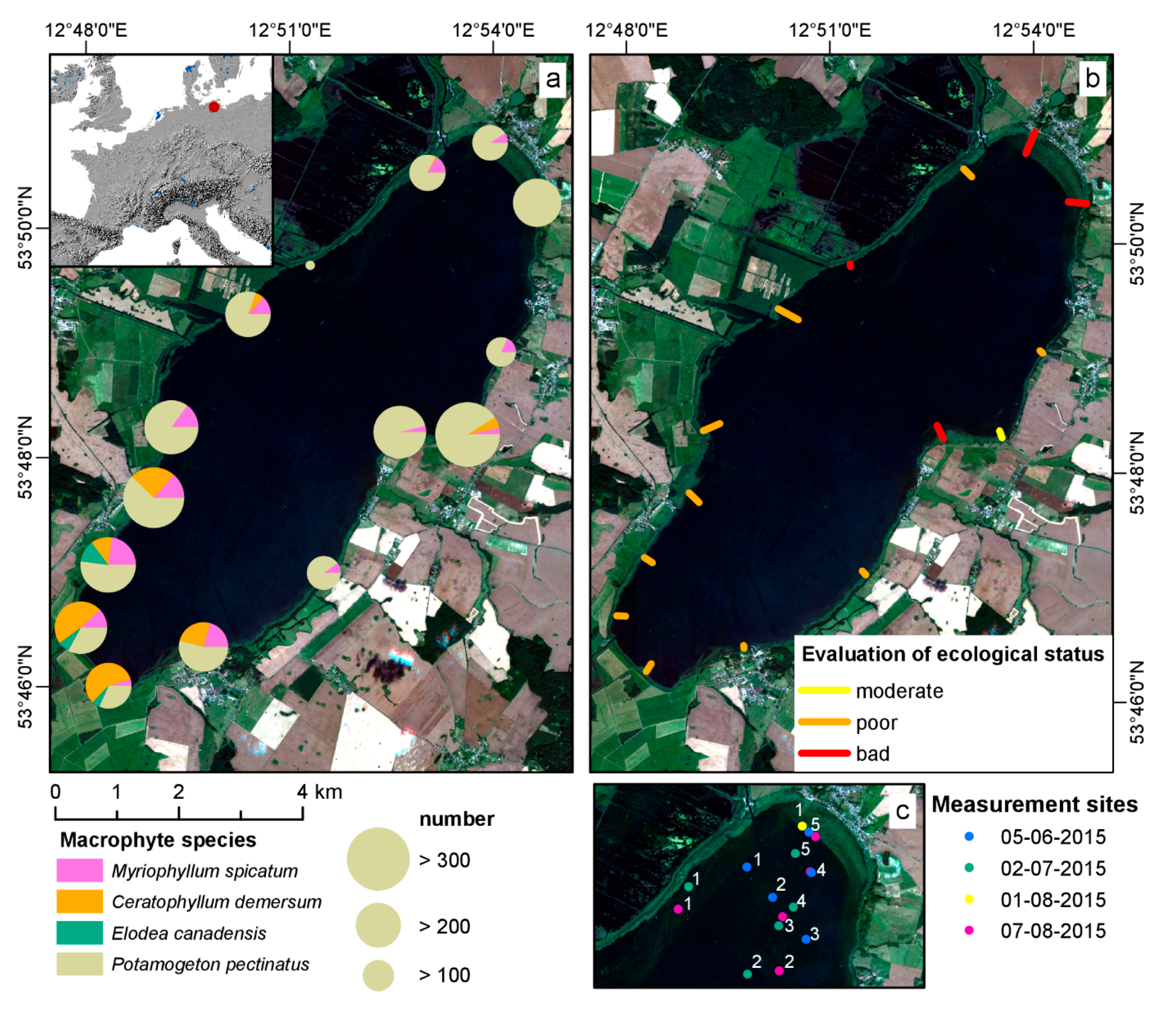
Figure 2.
Mean , retrieved from in situ measurements of Lake Kummerow for four RapidEye scenes. Error bars indicate standard deviation.
Figure 2.
Mean , retrieved from in situ measurements of Lake Kummerow for four RapidEye scenes. Error bars indicate standard deviation.

Figure 3.
(a) Irradiance reflectance of submerse aquatic vegetation (SAV) and bare sediment, measured ex situ and resampled to RapidEye. Error bars indicate standard deviation; (b) Depth-invariant indices for sediment and SAV for the different days, calculated according to the equation of Lyzenga [35] (Equation (5)).
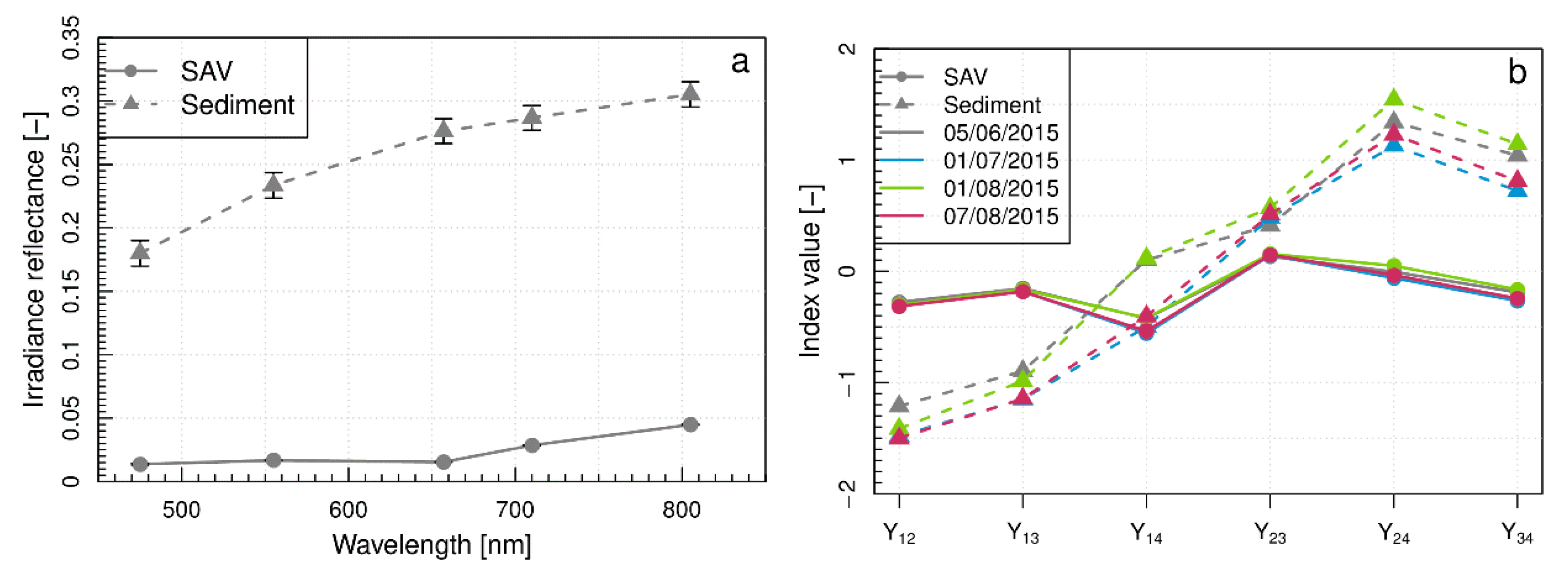
Figure 4.
Seasonal changes in littoral bottom coverage of Lake Kummerow (a) northern littoral; (b) illustrated by the depth-invariant index Y3,4; (c) 12 June 2015; (d) 1 July 2015; (e) 1 August 2015; (f) 7 August 2015. Bare sediment covered areas are displayed in red, dense SAV in green, mixed areas in yellow. Land and deep water areas are masked (except for 7 August 2015 where only land areas have been masked successfully), invalid pixels are displayed black. Contains material © (2015) Planet Labs. All rights reserved.

Figure 5.
Evaluation of SAV mapping with (a) In situ observed littoral bottom coverage highlighted in Google Earth imagery (acquisition date: 9 August, Image © 2017 TerraMetrics); (b) Reference areas based on Google Earth imagery and transferred to RapidEye (acquisition date: 1 August); (c) Categorised depth-invariant index Y3,4 of RapidEye data. Contains material © (2015) Planet Labs. All rights reserved.

Figure 6.
Comparison between resampled in situ measured median spectra and RapidEye 5 × 5 pixel environment mean spectra. Error bars indicate standard deviation (RapidEye) and 25% resp. 75% percentile (in-situ). (a) In situ data acquisition on 2 July and RapidEye acquisition on 1 July; (b) 1 August; (c) 7 August.


Table 1.
Settings of atmospheric correction, solar and sensor geometry and weather conditions close to image acquisition (±1 h).
Table 1.
Settings of atmospheric correction, solar and sensor geometry and weather conditions close to image acquisition (±1 h).
| Acquisition Date | Acquisition Time (UTC) | Satellite | Wind Direction [°] | Wind Speed [m s−1] | Solar Zenith [°] | Viewing Angle [°] | Aerosol Model | Calculated visibility [km] | In situ Data |
|---|---|---|---|---|---|---|---|---|---|
| 12 June 2015 | 10:53 | RE-3 | 50–80 | 2–3 | 30.6 | 12.9 | Maritime mid-latitude summer | 45.6 | −7 days |
| 1 July 2015 | 10:52 | RE-3 | 40–70 | 2–3 | 30.7 | 14.8 | Maritime mid-latitude summer | 111.7 | +1 day |
| 1 August 2015 | 11:03 | RE-5 | 60 | 2–5 | 35.7 | 2.9 | Maritime mid-latitude summer | 88.9 | +3 h |
| 7 August 2015 | 11:11 | RE-1 | 290–350 | 1–6 | 37.2 | 6.7 | Maritime mid-latitude summer | 25.1 | ±2 h |
Table 2.
Average water constituent concentrations and number of measurement points at in situ campaigns close or concurrently to RapidEye data acquisition.
Table 2.
Average water constituent concentrations and number of measurement points at in situ campaigns close or concurrently to RapidEye data acquisition.
| RapidEye Acquisition Date | In situ Data Collection | RAMSES Measurement Points | Secchi Depth [m] | SPM [g·m−3] | Chl-a [mg·m−3] | acDOM(440) [m−1] |
|---|---|---|---|---|---|---|
| 12 June 2015 | 5 June 2015 | 3 | 3.8 ± 0.3 | 0.7 ± 0.6 | 1.4 ± 0.3 | 1.38 ± 0.05 |
| 1 July 2015 | 2 July 2015 | 5 | 2.3 ± 0.7 | 1.3 ± 1.2 | 11.6 ± 4.1 | 1.28 ± 0.06 |
| 1 August 2015 | 1 August 2015 | 1 | No measurement | 0.7 ± 0.3 | 1.7 ± 1.8 | 1.28 ± 0.00 |
| 7 August 2015 | 7 August 2015 | 4 | 1.8 ± 0.5 | 3.6 ± 0.5 | 16.7 ± 2.9 | 1.27 ± 0.11 |
Table 3.
Error matrix and class accuracy measures of categorized Y3,4 (1 August) based on Google Earth imagery (9 August) reference data. The number of reference pixels is about 2.5% of the investigated area.
Table 3.
Error matrix and class accuracy measures of categorized Y3,4 (1 August) based on Google Earth imagery (9 August) reference data. The number of reference pixels is about 2.5% of the investigated area.
| Class | Reference Data (Number of Pixels) | User’s Accuracy [%] | |||||
|---|---|---|---|---|---|---|---|
| Dense SAV | Mixed SAV Dominated | Mixed Sediment Dominated | Pure Sediment | Sum | |||
| Depth-invariant index data [number of pixels] | dense SAV | 26 | 9 | 0 | 0 | 35 | 74.3 |
| mixed SAV dominated | 19 | 106 | 19 | 1 | 145 | 73.1 | |
| mixed Sediment dominated | 3 | 48 | 113 | 8 | 172 | 65.7 | |
| pure sediment | 0 | 1 | 25 | 101 | 127 | 79.5 | |
| Sum | 48 | 164 | 157 | 110 | 479 | ||
| Producer’s accuracy [%] | 54.2 | 64.6 | 72.0 | 91.8 | |||
| masked | 43 | 4 | 0 | 0 | 47 | ||
Table 4.
Accuracy measures of each measurement site calculated between corresponding RapidEye 5 × 5 pixel environment mean and resampled in situ measured median spectra (bands 1–4).
Table 4.
Accuracy measures of each measurement site calculated between corresponding RapidEye 5 × 5 pixel environment mean and resampled in situ measured median spectra (bands 1–4).
| RapidEye Acquisition Date | In situ Data Acquisition Date | Measurement Site | RMSE [sr−1] | r [-] | Percentage Bias [%] |
|---|---|---|---|---|---|
| 1 July 2015 | 2 July 2015 | 1 | 0.0017 | 0.82 | −32.2 |
| 1 July 2015 | 2 July 2015 | 2 | 0.0013 | 0.64 | 59.4 |
| 1 July 2015 | 2 July 2015 | 3 | 0.0006 | 0.81 | 3.8 |
| 1 July 2015 | 2 July 2015 | 4 | 0.0007 | 0.74 | 4.6 |
| 1 July 2015 | 2 July 2015 | 5 | 0.0007 | 0.74 | 0.6 |
| 1 August 2015 | 1 August 2015 | 1 | 0.0023 | 0.88 | −19.8 |
| 7 August 2015 | 7 August 2015 | 1 | 0.0067 | 0.68 | 281.1 |
| 7 August 2015 | 7 August 2015 | 2 | 0.0050 | 0.58 | 87.7 |
| 7 August 2015 | 7 August 2015 | 3 | 0.0071 | 0.52 | 252.2 |
| 7 August 2015 | 7 August 2015 | 4 | 0.0058 | 0.71 | 187.3 |
| 7 August 2015 | 7 August 2015 | 5 | 0.0026 | 0.95 | 27.7 |
Table 5.
Mean and standard deviation of AOT at 550 nm values retrieved from RapidEye data during ATCOR2 atmospheric correction in comparison to MODIS product AOT at 550 nm values [50,51] in a 3 × 3 (30 × 30 km2) pixel environment covering the study area.
| Date | MODIS Acquisition Time (UTC) | AOT MODIS | RapidEye Acquisition Time (UTC) | AOT ATCOR2 | RMSE [-] | Percentage Bias [%] | r [-] |
|---|---|---|---|---|---|---|---|
| 12 June 2015 | TE 10:25 | 0.119 ± 0.037 | 10:53 | 0.181 ± 0.005 | 0.072 | −13.5 | 0.94 |
| 12 June 2015 | AQ 12:10 | 0.174 ± 0.043 | 10:53 | 0.181 ± 0.005 | |||
| 1 July 2015 | TE 9:15 | 0.127 ± 0.019 | 10:52 | 0.116 ± 0.009 | |||
| 1 August 2015 | AQ 12:00 | 0.119 ± 0.048 | 11:03 | 0.102 ± 0.002 | |||
| 7 August 2015 | TE 11:15 | 0.390 ± 0.017 | 11:11 | 0.301 ± 0.003 | |||
| 7 August 2015 | AQ 13:00 | 0.437 ± 0.045 | 11:11 | 0.301 ± 0.003 |
© 2017 by the authors. Licensee MDPI, Basel, Switzerland. This article is an open access article distributed under the terms and conditions of the Creative Commons Attribution (CC BY) license (http://creativecommons.org/licenses/by/4.0/).
Share and Cite
MDPI and ACS Style
Fritz, C.; Dörnhöfer, K.; Schneider, T.; Geist, J.; Oppelt, N. Mapping Submerged Aquatic Vegetation Using RapidEye Satellite Data: The Example of Lake Kummerow (Germany). Water 2017, 9, 510. https://doi.org/10.3390/w9070510
AMA Style
Fritz C, Dörnhöfer K, Schneider T, Geist J, Oppelt N. Mapping Submerged Aquatic Vegetation Using RapidEye Satellite Data: The Example of Lake Kummerow (Germany). Water. 2017; 9(7):510. https://doi.org/10.3390/w9070510
Chicago/Turabian StyleFritz, Christine, Katja Dörnhöfer, Thomas Schneider, Juergen Geist, and Natascha Oppelt. 2017. "Mapping Submerged Aquatic Vegetation Using RapidEye Satellite Data: The Example of Lake Kummerow (Germany)" Water 9, no. 7: 510. https://doi.org/10.3390/w9070510
Note that from the first issue of 2016, this journal uses article numbers instead of page numbers. See further details here.