Article

Food Web Responses to Artificial Mixing in a Small Boreal Lake

1
Lammi Biological Station, University of Helsinki, FI-16900 Lammi, Finland
2
Natural Resources Institute Finland (Luke), FI-40500 Jyväskylä, Finland
3
Finnish Environment Institute (SYKE), FI-00250 Helsinki, FInland
4
Norwegian Water Resources and Energy Directorate (NVE), N-0368 Oslo, Norway
*
Author to whom correspondence should be addressed.
Water 2017, 9(7), 515; https://doi.org/10.3390/w9070515
Submission received: 27 April 2017 / Revised: 27 June 2017 / Accepted: 1 July 2017 / Published: 12 July 2017
(This article belongs to the Special Issue Ecological Responses of Lakes to Climate Change)

Abstract

:
In order to simulate food web responses of small boreal lakes to changes in thermal stratification due to global warming, a 4 year whole-lake manipulation experiment was performed. Within that time, period lake mixing was intensified artificially during two successive summers. Complementary data from a nearby lake of similar size and basic water chemistry were used as a reference. Phytoplankton biomass and chlorophyll a did not respond to the greater mixing depth but an increase was observed in the proportional abundance of diatoms, and the proportional abundance of cryptophytes also increased immediately after the onset of mixing. Obligate anoxic green sulphur bacteria vanished at the onset of mixing but gradually recovered after re-establishment of hypolimnetic anoxic conditions. No major effect on crustacean zooplankton was found, but their diversity increased in the metalimnion. During the mixing, the density of rotifers declined but protozoan density increased in the hypolimnion. Littoral benthic invertebrate density increased during the mixing due to Ephemeroptera, Asellus aquaticus and Chironomidae, whereas the density of Chaoborus larvae declined during mixing and lower densities were still recorded one year after the treatment. No structural changes in fish community were found although gillnet catches increased after the onset of the study. The early growth of perch (Perca fluviatilis) increased compared to the years before the mixing and in comparison to the reference lake, suggesting improved food availability in the experimental lake. Although several food web responses to the greater mixing depth were found, their persistence and ecological significance were strongly dependent on the extent of the disturbance. To better understand the impacts of wind stress on small lakes, long term whole-lake experiments are needed.

1. Introduction

The thermal conditions of lakes are determined mostly by meteorological forcing at the air-water interface [1,2]. Air temperature and wind velocity are the most important meteorological variables determining the heat balance in lakes. Seasonal and inter-annual changes in the weather therefore have a major impact on the thermal characteristics of lakes. However, lakes with contrasting morphometry may respond differently to changes in weather [3,4]. For example, deep lakes with large water volume integrate the effects of meteorological forcing over longer time periods than shallow lakes. Other important factors that influence the thermal characteristics of lakes include water residence time, optical properties and landscape setting [3,5,6]. These factors also regulate patterns of spatial coherence in the thermal conditions of lakes [7].
Small lakes are numerous in the northern hemisphere, and particularly in the taiga and tundra areas [8], where their role in the global carbon cycle has been proven to be much bigger than was earlier expected [9]. These northern areas are also expected to face rapid warming due to global climate change, a major driver which already influences water bodies and their thermal characteristics at a multicontinental scale [10]. However, relatively little information is available on boreal lakes and their ecosystem responses to warmer climatic conditions, such as changes in water-column stability and stratification. The main body of information regarding ecosystem responses is based on empirical long-term studies [11,12,13,14,15], while up to now there have been only a few experimental and modelling studies on the topic [16,17,18,19].
Lakes in northern Europe and other temperate and boreal regions of the world are predominantly dimictic, meaning that annually the lakes have two circulation periods (spring and autumn) and two stratification periods (summer and winter). In summer, when the lakes are free of ice, even minor changes in wind velocity and temperature regimes may affect their thermal stratification. A change in the thermal regime of a lake can affect ecosystem function and structure at different trophic levels [11,12,17,19]. For northern Europe, recent climate change scenarios predict increases in precipitation and air temperature [20], both in winter and in summer. In addition, there are indications that storminess has increased over the past century in northern and north-western Europe (European Environment Agency), which will increase extreme wind velocities as well as mean geostrophic wind in the north. These changes can be expected to result in an increase in the mixing energy in lakes. Hence we conducted a 4 year whole-lake manipulation experiment in Lake Halsjärvi, in southern Finland [21,22,23]. The experiment was carried out in collaboration with the EU project “Integrated Project to evaluate the Impacts of Global Change on European Freshwater Ecosystems”. The rationale was to manipulate the thermal stratification patterns and heat balance artificially by increasing the input of mixing energy to the lake [21]. The manipulation experiment was expected to provide valuable information on the effects of wind mixing on small boreal lake ecosystems in particular. Our thermocline manipulation followed the same experimental design (THERMOS) as was earlier applied in Norway [17].
Our primary aim was to study how the ecosystem of a small boreal lake responds to artificial mixing and subsequent change in the thermal and chemical stratification patterns. The ecological responses and possible consequences for ecosystem services were illustrated by measuring ecosystem metabolic processes and the food web structure related to changes in the physical and chemical conditions. We focused on the following questions. Firstly, does the greater mixing depth affect the community structure of phytoplankton and zooplankton, and the metabolism of phytoplankton and bacterioplankton. Secondly, if better oxygen conditions prevail in the lake, does the abundance of benthic invertebrates increase and community structure change? Thirdly, how may photosynthetic green sulphur bacteria (obligate anoxic organisms) respond to the mixing when in similar small humic lakes they occur close to the boundary layer between the metalimnion and hypolimnion [24]. Fourthly, are cascading effects apparent at the top of the food chain such as the growth of fish and their methyl-Hg concentrations [25].
We also compare our results with those from the THERMOS experiment in Norway [17] and the TIMEX experiment in Canada [19,25,26,27]. In the context of climate change impacts on lake ecosystems, whole-lake manipulation experiments provide unique material for upscaling ecosystem responses to thermocline deepening by combining abiotic and biotic processes and their interactions at varying temporal and spatial scales. When all lakes have their own specific characteristics, depending, for example, on their morphometry and geographical location, and landscape position, results from various ecosystems and processes are needed for more comprehensive understanding of lake responses to changes in climatic conditions, including wind stress.

2. Materials and Methods

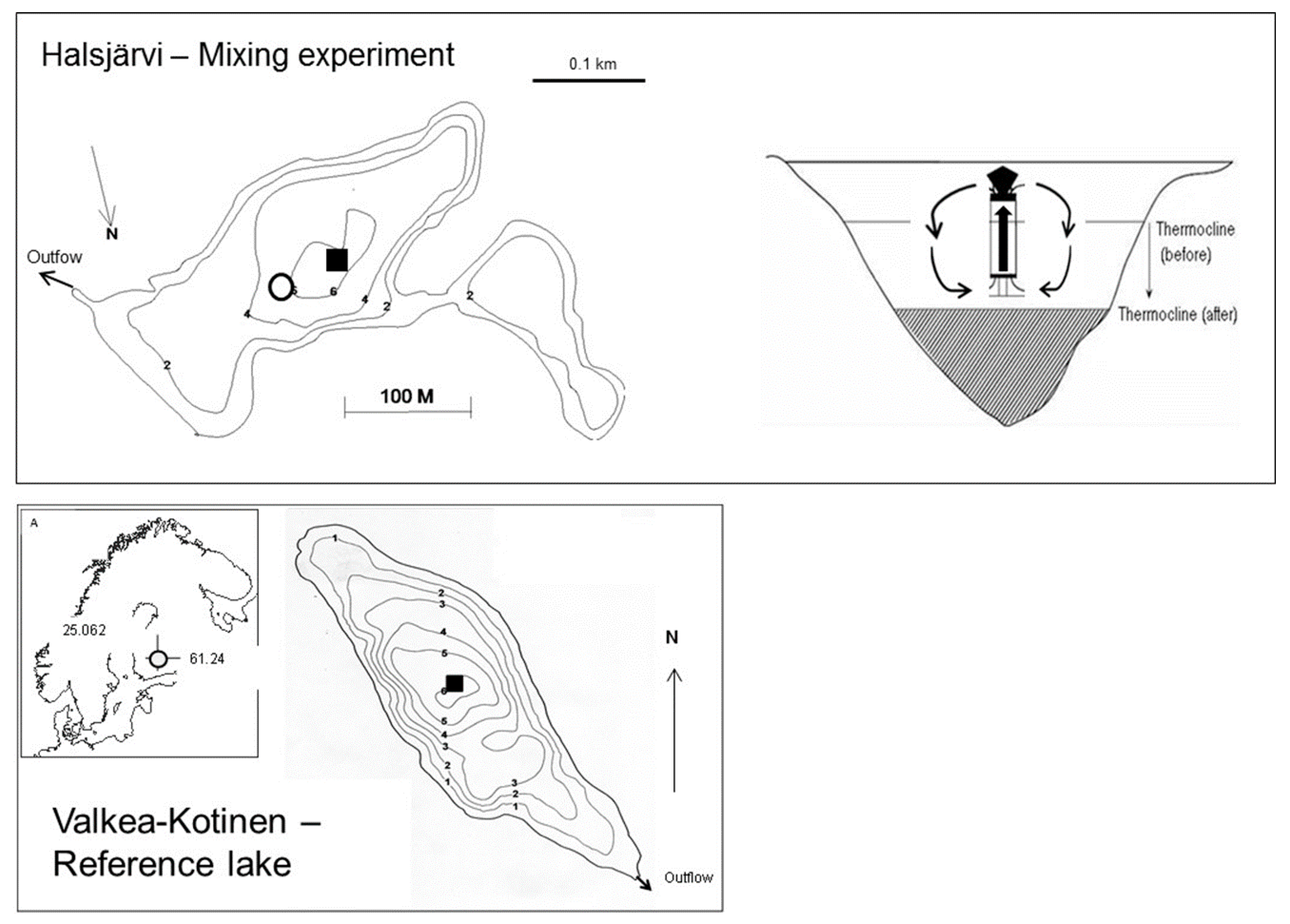
2.1. Lake Characteristics and Experimental Design

The results of this study are based on a whole-lake experiment which was carried out in Halsjärvi, a small humic lake in southern Finland (Figure 1), in 2004–2007. The mixing manipulation was performed in 2005–2006, so besides after the manipulation period, data are also available from one antecedent and subsequent summer seasons. In addition, we gathered similar physical, chemical and biological data from a nearby lake (Valkea-Kotinen). This information is used as a reference for considering the ecosystem responses to the artificial mixing. Basic information about both the study lake and the reference is provided in Table 1.
Many results from our experiment have already been published, including a thermodynamic model [MyLake] application for ecological forecasting [18], physical and chemical responses to the manipulation [21], effects on mercury methylation [23] and methyl mercury concentrations in fish [22]. In this paper, we focus on the metabolic and food web responses of the manipulation. More information about the physical, chemical and biological characteristics of the reference lake, Valkea-Kotinen (Table 1 and Figure 1), including biogeochemical processes and long-term changes, are given in the following publications [28,29,30,31]. Both lakes have high dissolved organic carbon content due to high load of allochthonous humic substances, a characteristic feature for small lakes in the region [4,7,32]. Both lakes are influenced by similar meteorological drivers, because they are close to each other (distance is 4.5 km; for more information on the climate and deposition of the area) [33,34].
The mixing was achieved by using a modified commercial aeration equipment (MIXOX, Water-Eco Ltd., Kuopio, Finland) by means of an electrically-driven propeller positioned at 1.5 m depth below a raft anchored at the deepest point of the lake, and by pumping water from the metalimnion into the epilimnion (for more details of the experimental design and technical issues, see [18,21]). The artificial mixing started in the lake at the end of May 2005 and in that year mixing finished at the beginning of September, when autumnal turn-over usually starts. In 2006, mixing started at the beginning of June and finished at the beginning of September. Artificial mixing was intended to increase the depth of thermocline by 1 to 1.5 m (Figure 2 and Figure 3), a change which was selected to correspond to the projected increase in the mean temperature of the lake at the end of the 21st century due to climate warming.

2.2. General Aspects of Sampling

The study lakes were sampled weekly in 2004–2006 and every two weeks in 2007. Samples for water chemistry and plankton biology were taken from the deepest point of each lake which is almost in the middle of both water bodies (Figure 1). Measurements from entire water columns for in situ profiles of water temperature (Tw) and dissolved oxygen (DO) concentrations were taken from the middle of the lakes by YSI 55 combined temperature-oxygen meter (Yellow Springs Instruments Inc., Yellow Springs, OH, USA). In both lakes a thermistor chain (Minilog data loggers) was also placed at the deepest point. The epilimnion, metalimnion and hypolimnion sampling depths were chosen each time based on Tw and DO profile measurements. Samples were collected with 0.3 m long (volume 2.4 L) Limnos tube samplers (except for zooplankton, see below), depending on the stratification and purpose of the samples (water chemistry vs. metabolic measurements). Each water layer was sampled from top to bottom, thus producing a composite sample. As a result, the collected water volumes varied a lot between different layers and sampling times, although the final subsamples for water chemistry (pH, alkalinity, conductivity, colour, TOC/DOC, TP, TN, PO4-P, NO3-N, NH4-N, cations, and chlorophyll a and d) and biological measurements (densities and biomasses of organisms as well as primary production and respiration of plankton) were the same. During the homothermal periods an integrated sample from the whole water column was also taken for chemistry. In the reference lake samples for water chemistry and biology were taken from the entire water column [for zooplankton] or from different depths as a one meter composite samples, except that samples for metabolic measurements were taken from several narrow water layers from the surface down to the metalimnion or hypolimnion. However, in this article only the epilimnetic samples from the reference lake were analyzed for comparison purposes except in the case of zooplankton. It should be noted that the water-column of the reference lake is even more steeply stratified than in the experimental lake, and thus the depth of the photic zone is only approximately 1 m and below that depth anoxia commonly prevails in summer [28,31].
At the very beginning of the mixing treatment in 2005 the water column was completely overturned due to too high pumping power. Although the power was almost immediately reduced by changing the pumping direction from top down to bottom up, it took some weeks for thermal and chemical stratifications to re-form (for more details on the thermal chemical conditions, see [21]). Although artificial mixing induced some chemical responses in the lake [21], only the key results necessary for interpreting the food web responses are briefly mentioned in this context.
However, before any chemical responses caused by the mixing manipulation, we need to look at the chemical changes which originated already in 2004 due to the exceptionally wet summer season. During a period of seven weeks from 12 June precipitation was nearly 350 mm, which is the highest ever measured summer precipitation in 1963 when the measurements started in the area. As a consequence, surface and subsurface runoff dramatically increased and the groundwater table also reached its maximum level [35]. Because of increased runoff the lakes received high load of inorganic nutrients and organic matter from their catchment areas [28,31]. Therefore, epilimnetic DOC, colour, TP, TN, NO3, NH4 and Fe concentrations increased 2- to 4-fold until the middle of August compared to the early June [21]. As a result of the increase in colour and DOC, light penetration into the lake radically diminished. The following year when the artificial mixing enhanced the depth of the epilimnion, high colour and DOC concentrations were found in the lake. As a result of the greater mixing depth and enhanced light attenuation the euphotic zone then represented only 50% of the epilimnion. When colour values gradually decreased in the course of the two summer seasons with artificial mixing, light conditions simultaneously improved. However, a major change in photic conditions only appeared in 2007 after the mixing treatment was finished.

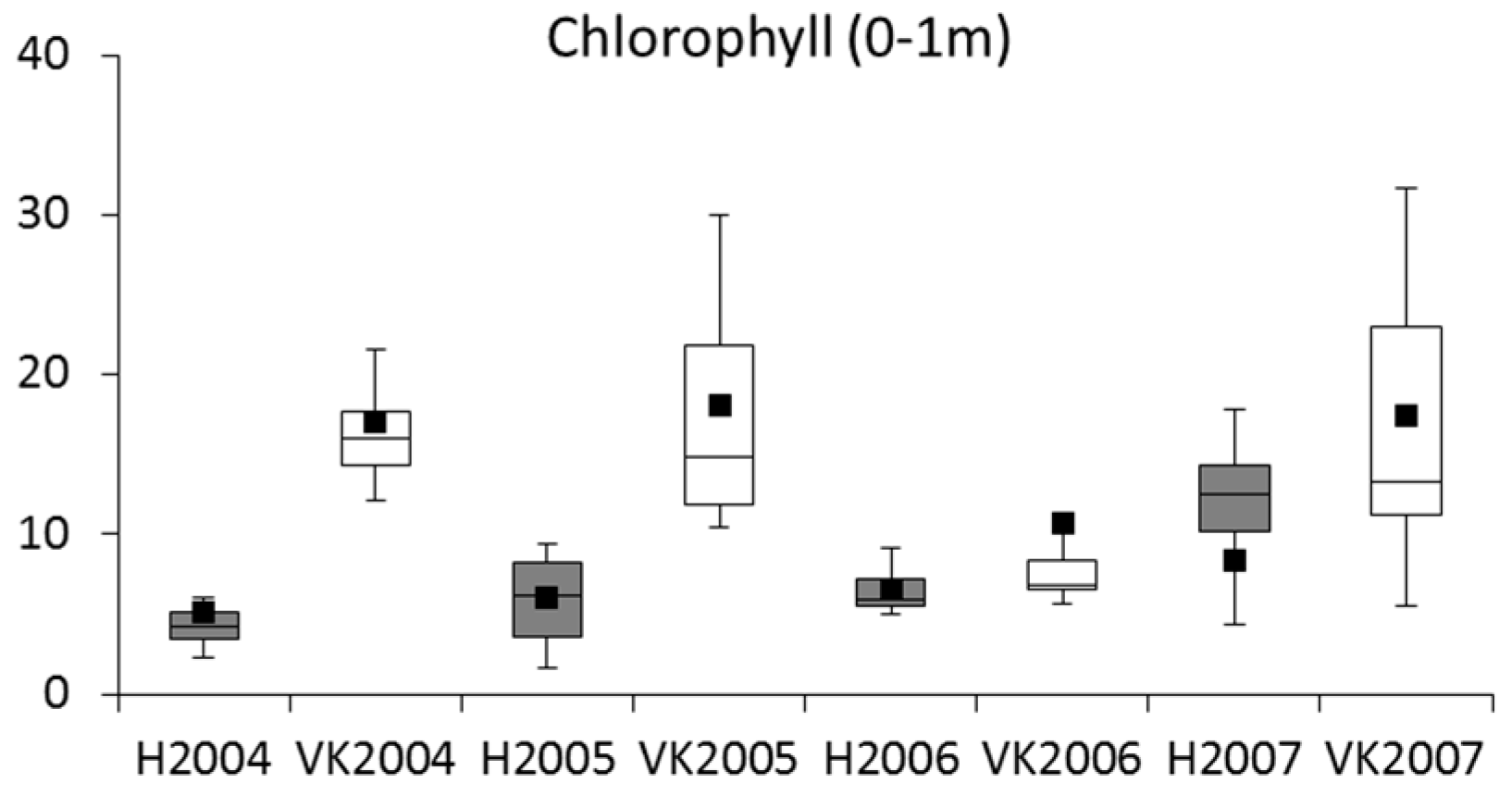
2.3. Chlorophyll Analyses

Analysis of chlorophyll a and bacteriochlorophyll d, indicators of phytoplankton and green sulphur bacteria were made by hot ethanol extraction and the role of different pigments was estimated based on the absorbance ratio method [24]. All chemical analyses were made according to the standard methods [28,31] at the laboratory of the Lammi Biological Station, University of Helsinki. Phytoplankton samples were preserved by acid Lugol’s solution and later counted by inverted microscope with 300× and 600× of magnification [36].

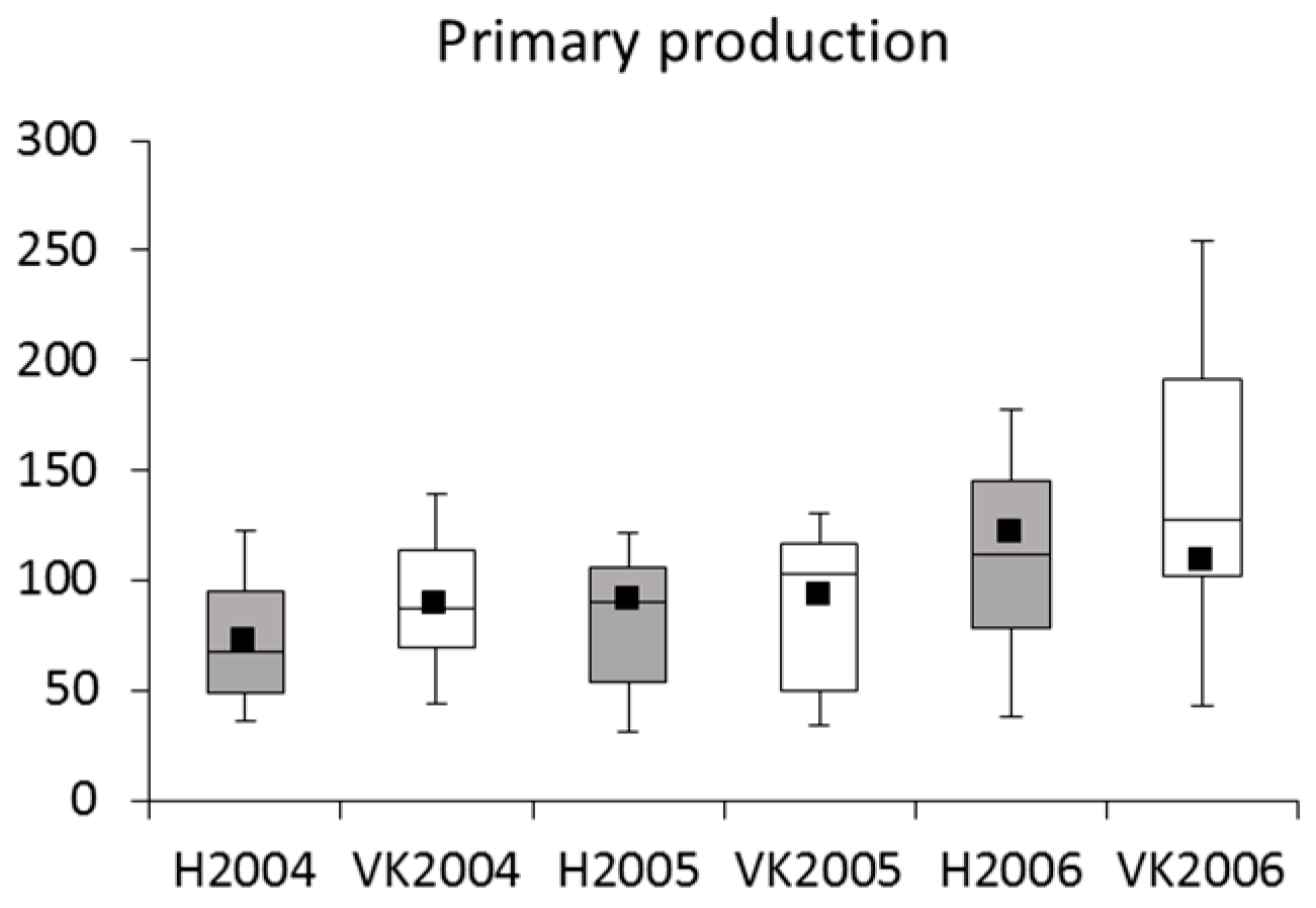
2.4. Primary Production

Primary production was determined using an acidification and bubbling modification of the 14C-method with a 24 h in situ incubation in light bottles [28]. Respiration of plankton was determined as the increase in dissolved inorganic carbon (DIC) in dark bottles during 24 h in situ incubation. DIC was determined with the acidification and bubbling method [37].

2.5. Zooplankton

Zooplankton samples were taken with a 1-m-long 6.5 L tube sampler from the surface down to 5 m depth at 1 m intervals. Sample water was sieved through a 50 µm mesh plankton net before preservation of the zooplankton samples by formaldehyde solution (final concentration 10%). Zooplankton were counted and results calculated as densities (ind.·L−1) [29,38].

2.6. Benthic Macroinvertebrates

The benthic macroinvertebrate samples were taken with a tube sampler of 64 cm2 from three littoral (0–1 m) sampling points and by a tube sampler of 54 cm2 from three profundal (6 m) sampling points. In both lakes the samples were taken in September 2004–2007. Five lifts per sampling point were pooled to make a single sample. The area of one sample was considered to be 318 cm2 in the littoral and 270 cm2 in the profundal zone. The samples were sieved through a 0.5 mm mesh net, animals were picked out and identified to major taxonomic groups and densities (ind.·m−2) and biomasses (g·m−2, ww) were calculated [38].

2.7. Fish

Fish community structure was examined during 2004–2008 in both lakes using Nordic multi-mesh survey nets [39,40] with an effort of eight nets in both lakes each year. To examine possible responses of fish growth to the thermocline manipulation, the age of perch was determined and 1st and 2nd year growth back-calculated for the years 2002–2007 from opercular bones according to Monastyrsky’s procedure [41,42].

2.8. Statistical Analyses

Randomized Intervention Analysis (RIA), Ref. [43,44] was used to test for statistical significance of changes that can be ascribed to the manipulation. The RIA method is designed specifically for paired-ecosystem experiments, in which one ecosystem is manipulated while the other serves as a reference. The method does not assume that the two lakes are identical, but rather that both lakes respond similarly to natural fluctuations. The method requires a pre-treatment monitoring period during which the inherent difference between the lakes is determined, and then a treatment monitoring period. The method tests the hypothesis that the difference between the lakes changed when the treatment was initiated. In this study, RIA was used to compare paired, chronologically-ordered samples for the four-year data record of phytoplankton and zooplankton (one year pre-treatment, two years treatment, one year post-treatment) from the manipulated (Halsjärvi) and reference (Valkea-Kotinen) lakes. The RIA was done separately for the pre- and post-treatment periods. For the pre-treatment period only values for the year 2004 were used. Calculations of RIA were conducted in SAS 9.4 (SAS Institute, Cary, NC, USA). For other statistical tests, parametric and nonparametric according to the data properties, and for production of graphs, SigmaStat12.5, SPSS, SYSTAT 13 and Real Statistic soft-wares were used.

2.9. Supplementary Materials

Supplementary data are given in Tables S1–S7.

3. Results

3.1. Photosynthetic Bacteria

In summer 2005 bacteriochlorophyll d (BChl d) concentration, an indicator of green sulphur bacteria (GSB), collapsed in the hypolimnion of the study lake immediately after the onset of the mixing, and the concentration stayed low (<9.5 mg·m−3) in comparison to the other summer seasons (>25 mg·m−3, Figure 4). In 2006 the concentration was at the same level as that before and after the mixing experiment. The occurrence of GSB correlated negatively with hypolimnetic DO and SO4 concentrations.
In the hypolimnion of the reference lake, no equivalent decline in BChl d concentration and absorbance ratio (665:654 nm) took place in summer 2005. According to RIA analyses, the mixing induced changes in BChl d concentrations were significant (p < 0.01) when the entire water column in the study lake was considered (Table 2).

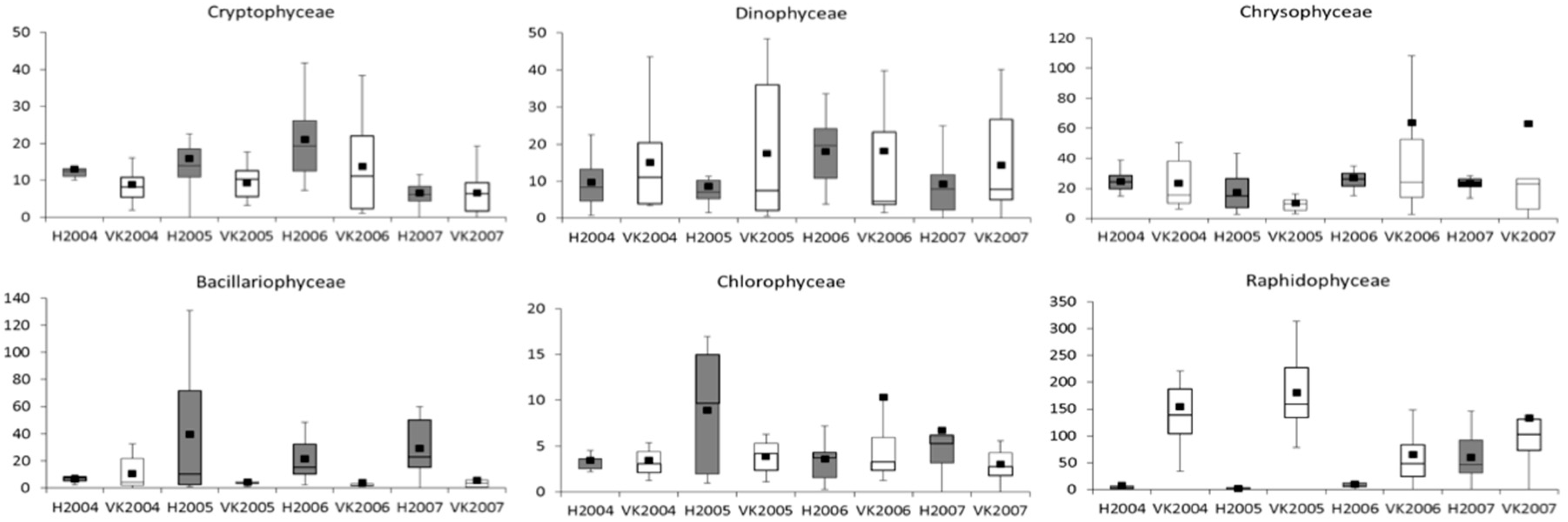
3.2. Phytoplankton and Metabolic Processes
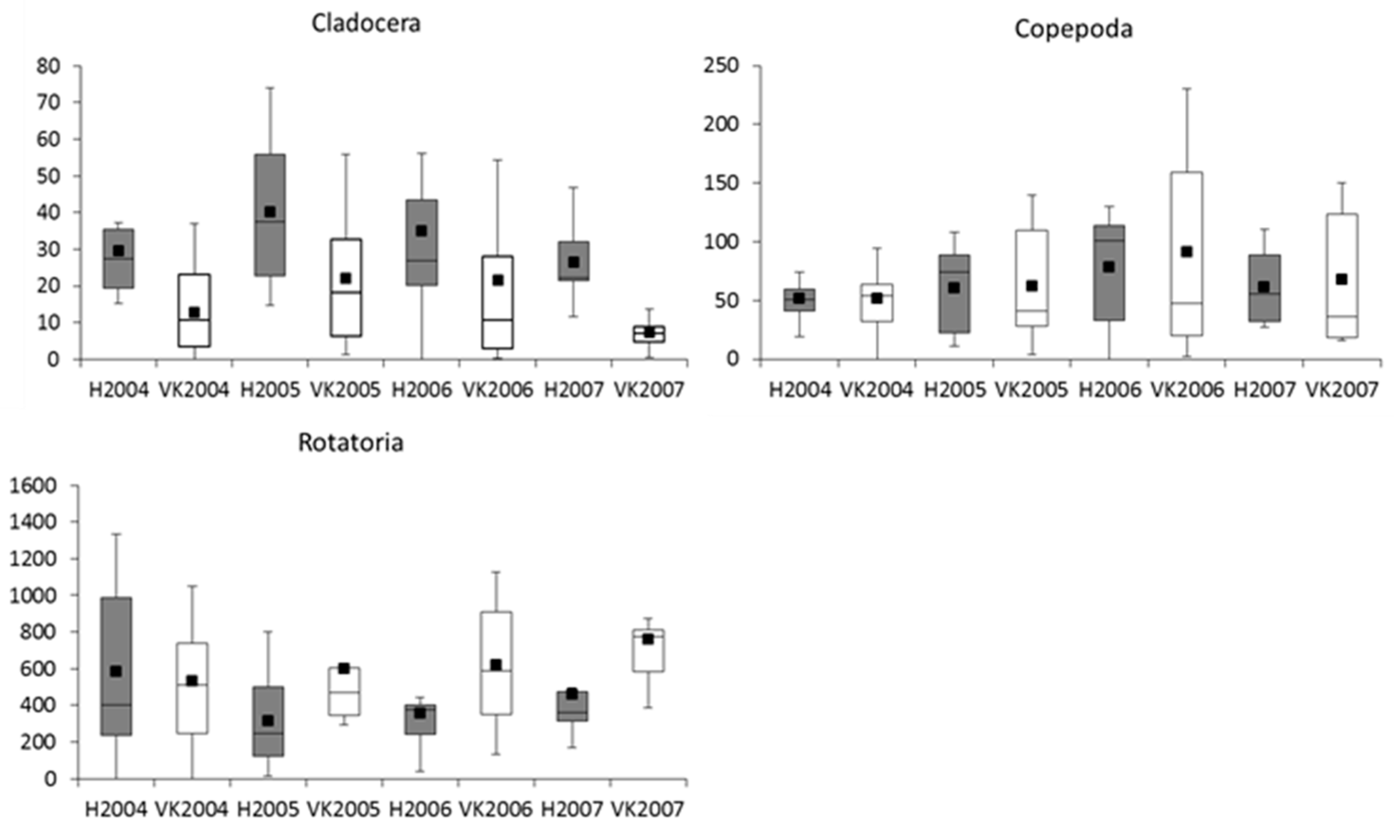
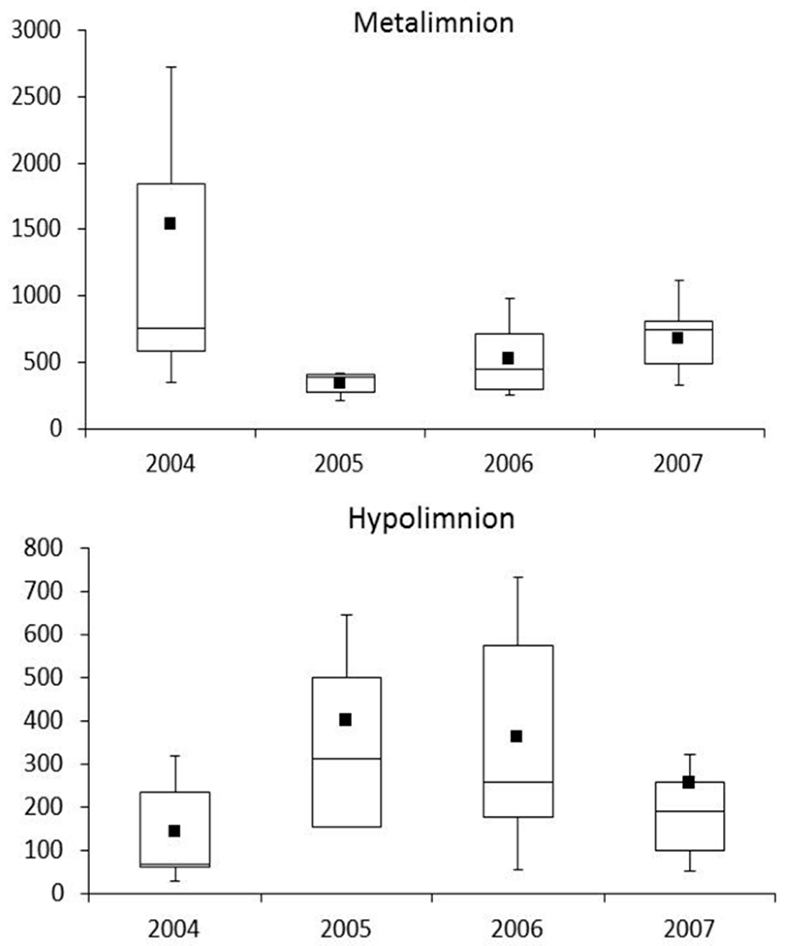
In the study lake, in summer 2005 the biomass of diatoms contributed 27% of the phytoplankton biomass, which was twice that in 2004, and in July–August, in particular, clearly higher than in the post-treatment year (2.4-times higher) and in the reference lake (see also Figure 5 with data for June–September). According to RIA analyses, the response was significant (p < 0.01) when the pre-treatment year was considered (Table 2). The biomass of Asterionella ralfsii, Fragilaria sp. and Aulacoseira distans in particular increased. The biomass of non-flagellated green algae (data not shown) increased in synchrony with diatoms and in 2006 the biomass of both groups was still above that in the period before mixing. Monoraphidium dybowskii, a common non-flagellate green alga, had clearly higher biomass during the artificial mixing than before or after the treatment. Along with Diatomophyceae, the response of Cryptophyceae to mixing was statistically significant (RIA, p < 0.05). In 2004–2007 Gonyostomum semen (Raphidophyceae) constituted, on average, 17% of phytoplankton biomass while during the manipulation experiment its share dropped down to 4% in 2005 and to 9% in 2006. In the reference lake its contribution was higher, and was highest (on average 74%) in summer 2005. In the metalimnion and hypolimnion phytoplankton biomasses showed no response to the mixing.
Despite these changes in the share of different taxonomic groups of algae to the total phytoplankton biomass, no major changes in chlorophyll a concentrations (Figure 6) could be found (RIA for epilimnion of Halsjärvi and 0–1 m depth of Valkea-Kotinen, Table 2). The only indication that mixing influenced phytoplankton biomass in the study lake was the slightly increasing trend of chlorophyll a since 2004.
The differences in primary production among the years were significant (Kruskal-Wallis test, p < 0.05) only at the 0.5 m and 1 m depths. In the reference lake PP remained at the same level with no significant differences between the three summer seasons. During the summer seasons (June tomid September) the mean PP varied in Halsjärvi varied between 72–122 mg·C·m−2·d−1 and in Valkea-Kotinen between 83–94 mg·C·m−2·d−1 (Figure 7).
In Halsjärvi summer respiration of plankton (June to mid September) varied between 268 and 334 mg·C·m−2·d−1, but the differences between the seasons were not significant. In the reference lake respiration was lower varying between 117 and 202 mg·C·m−2·d−1, and in 2005 it was significantly lower (t-test, p < 0.05) than in 2004 and 2006.

3.3. Zooplankton

For the two major taxonomic groups of zooplankton, rotifers and crustaceans, slight responses to the artificial mixing were recorded in the average densities in the entire water column. Rotifer densities were lower in 2005 and 2006 than before the treatment indicating a statistically significant response to the mixing (RIA, p < 0.05, Table 2, Figure 8 and Figure 9). No significant responses were detected in the main groups of crustaceans (Table 2). Cladoceran densities were somewhat higher during the mixing of the study lake (Figure 8) but due to wide within-year variation the differences were not significant. Among the cladocerans, non-significant responses were detected as the densities of Bosmina sp. and Daphnia sp. slightly decreased whereas the density of Ceriodaphnia sp. increased. Differences in copepods were also small between lakes as well as between years when mean densities of the whole water column were considered (Figure 8). However, in the hypolimnion of Halsjärvi the densities of cladocerans and calanoid copepods were distinctly (t-test, p < 0.05) higher especially during the first mixing summer season than during the summer before and after the treatment.
The summer average number of cladoceran taxa varied in the epilimnion between 5.6 and 6.8, being highest in 2007 and lowest in 2004, and that of rotifers varied between 16 and 20, being lowest in 2005 and highest in 2007. The lowest species richness was always found in the hypolimnion. In all three water layers the number of rotifer taxa gradually increased from 2005.
During the mixing in 2005 and 2006 the density of protozoans increased significantly in the hypolimnion (Figure 10), and to some extent also in the metalimnion and epilimnion, which might be connected to the decrease in Chaoborus larvae in the water column (Figure 10).

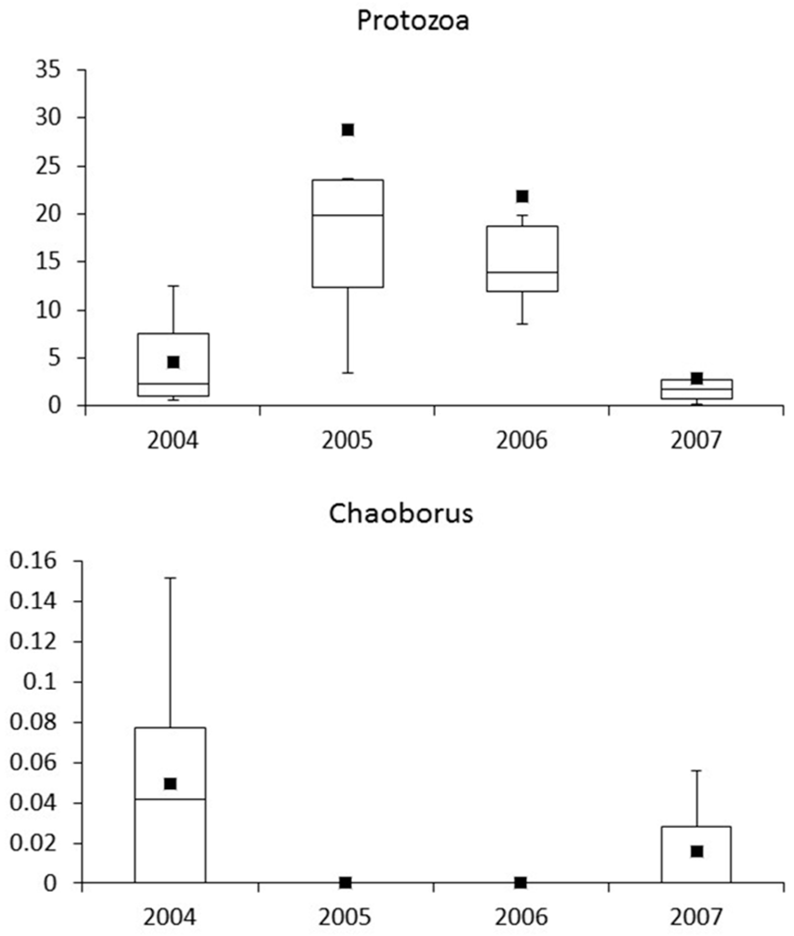
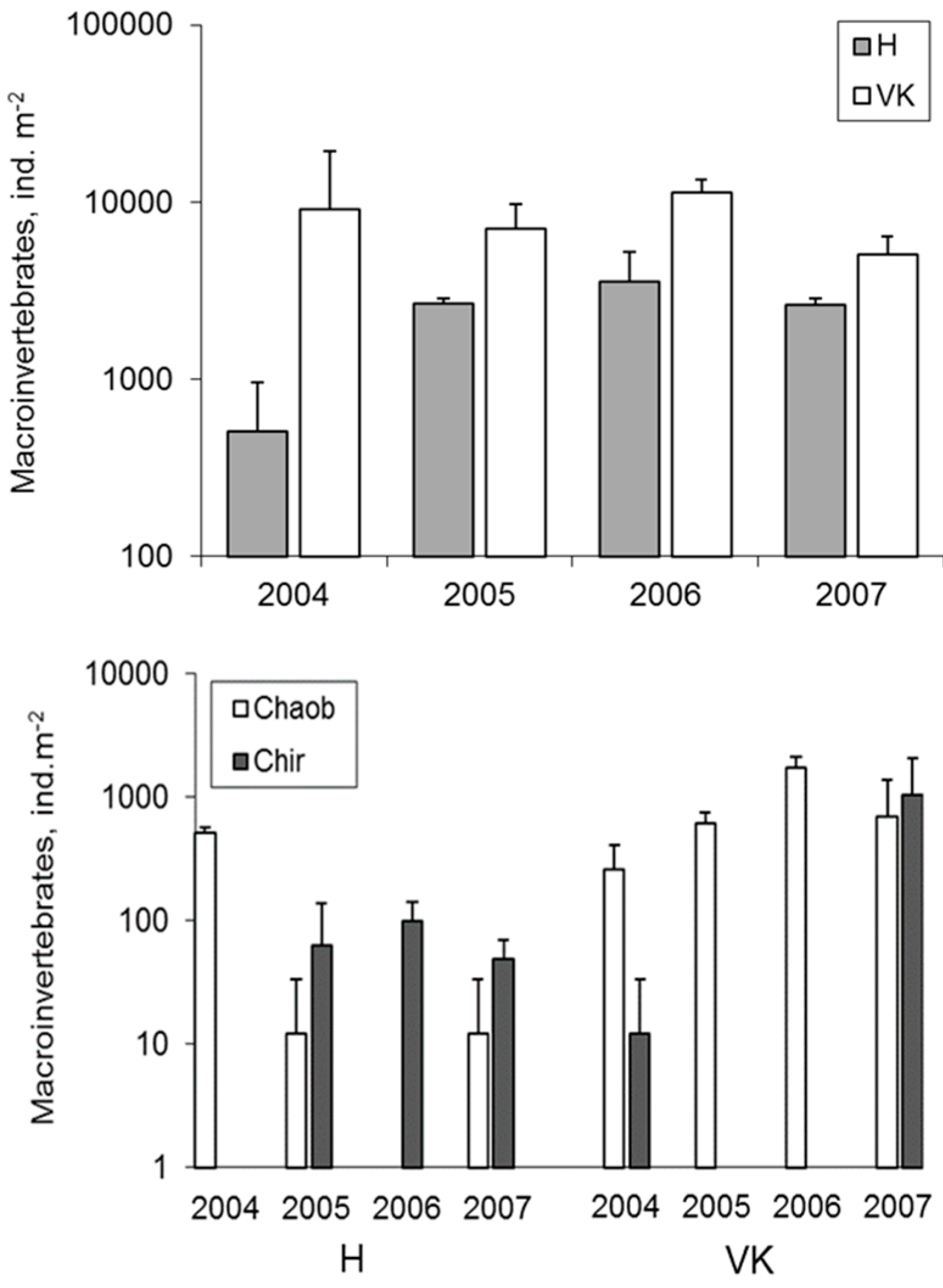
3.4. Macroinvertebrates
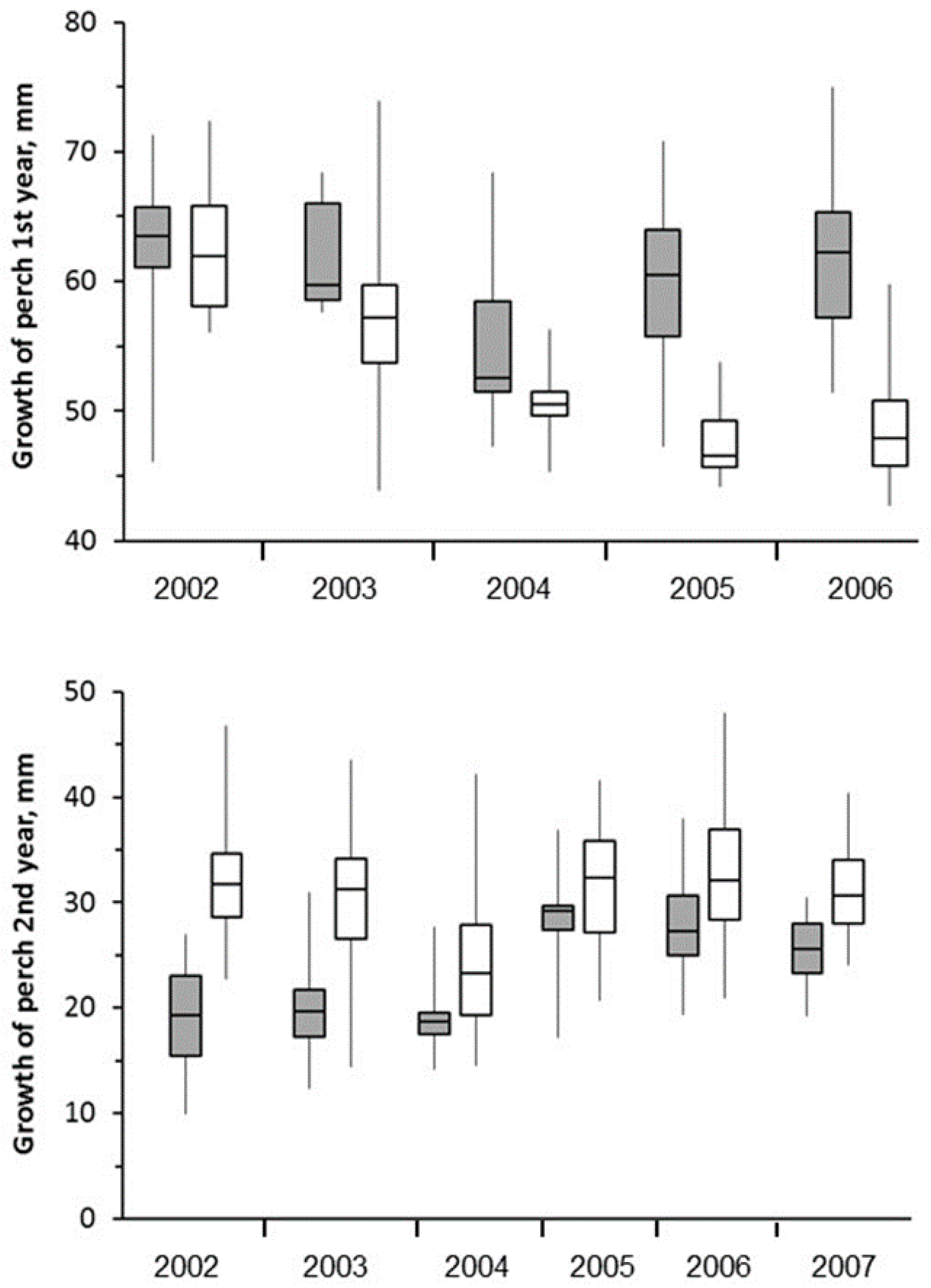
Among the littoral macroinvertebrates, Ephemeroptera, Chironomidae and Asellus aquaticus were numerically the most abundant taxonomic groups (Table 3). On average, the annual mean total densities of macroinvertebrates were distinctly lower in the study lake (500–3600 ind.·m−2) than in the reference lake (5100–11,300 ind.·m−2), mainly due to almost an order of magnitude higher densities of chironomid larvae in the reference lake (Table 3). The annual mean biomasses varied between 5.9–8.2 g·m−2 (ww) and 9.1–15.9 g·m−2 (ww), respectively.
During the artificial mixing in 2005–2006, the total density of littoral macroinvertebrates (Figure 11) of Halsjärvi was significantly higher than in the year before the mixing (Table 3). Only a few significant differences were recorded among taxonomic groups, (Ephemeroptera and Trichoptera). In some cases the lack of significance was at least partly because of wide within and between year variation. The highest littoral macroinvertebrate density in the reference lake occurred in 2006 and no significant between-year differences were found, except for chironomid larvae (Table 3). Total biomass of littoral macroinvertebrates did not show any response to the mixing, mainly due to the irregular occurrence of large Odonata nymphs.
In the profundal of the study lake, the mean total density of macroinvertebrates varied between 100–500 ind.·m−2 and in the reference lake between 360–3100 ind.·m−2. The mean biomasses were 0.3–1.5 g·m−2 (ww) and 0.7–8.2 g·m−2 (ww), respectively. Chaoboridae larvae were dominant in both lakes but in the study lake their density decreased sharply in 2005 and 2006 both in the water column (Figure 10) and at the bottom (Figure 11). In contrast, Chironomidae larvae appeared in the profundal samples in autumn 2005, after the first summer of mixing, and were present to the end of the study although in low numbers (Figure 11). Chironomids were also found occasionally in the profundal of the reference lake, and in 2007 their mean density reached a level of 1100 ind.·m−2, probably due to complete mixing of water column in spring 2007 (Figure 3).

3.5. Fish

The fish community in the study lake consisted of European perch (Perca fluviatilis), ruffe, (Gymnocephalus cernuus), northern pike (Esox lucius), roach (Rutilus rutilus), bleak (Alburnus alburnus) and bream (Abramis brama) while in the reference lake only perch and pike were present. The mean annual gillnet catches from both lakes varied between 6–36 fish individuals and 200–600 g of fish per net with an increasing but not significant trend (Figure 12).
Roach was the dominant species in the study lake making up 66–79% of the numerical catch and 48–59% of the biomass catch of gillnets. The corresponding proportions for perch were 19–30% and 8–32%. Ruffe appeared in the catches of the manipulated lake during the second year of mixing in 2006. Perch dominated the gillnet catches of the reference lake.
The back-calculated length at age 1 values for perch prior to the mixing in 2002–2004 decreased from levels of 60–65 mm to 50–55 mm in both lakes with no statistically significant difference between the lakes (Figure 13). During the mixing in 2005 and in 2006, the first year growth of perch returned to 60–65 mm in the study lake but not in the control lake. The second year growth of perch was significantly higher in the control lake than in the study lake before the mixing (Figure 13). Since the mixing was started the second year growth in the study lake increased but still remained lower than in the control lake.

4. Discussion

In our study, lake the food web responses to thermocline manipulation were complicated and extended to all trophic levels from bacteria to fish (Table 4), implying that a permanent change in the mixing efficiency and in the thermal stratification can cause major and irreversible changes in the entire food web. In small humic lakes, such as in Halsjärvi and Valkea-Kotinen, the thermocline determines the depth of the chemocline and the upper level of the anoxic water layer. In such lakes decomposition typically exceeds primary production of plankton [28,45,46], and may result in an extremely shallow (<1–2 m) oxic water layer in lakes smaller than just a few hectares in size. However, during the autumnal and vernal mixing periods, and occasionally during heavy storms in summer, the physical and chemical gradients may break down, so organisms inhabiting these ecosystems have to tolerate rapid changes in stratification. In summer, predators and prey are spatially very close to each other in such lakes [47,48,49,50,51,52], and also dependent on the boundaries between the different water layers.
In Lake Breisjøen, a deep oligotrophic clear water lake in Norway subjected to an almost identical experimental approach as in Lake Halsjärvi, a 3-year artificial thermocline deepening did not cause any major changes in water chemistry, phytoplankton, macrophyte and zooplankton communities, or fish populations [17], indicating that responses to thermocline manipulation depends on lake type.
The TIMEX manipulation in Canada, in turn, promoted top-down (predation) effects that increased over the 2 years of the experiment. Due to mixing there was a loss of hypolimnetic refuge for zooplankton, which in turn accentuated stronger predation by fish on larger cladocerans, and subsequent changes (decline) in mean community body size of zooplankton, and an increase in zooplankton biomass [19].

4.1. Responses of GSB

The boundary layers can be important microhabitats, which support phototrophic green sulphur bacteria (GSB) [24,49], methanotrophic bacteria [53], several protozoan species [54], and processes such as mercury methylation [23]. Besides anoxic conditions, other necessary requirements for GSB include hydrogen sulphide and solar energy which they need for photosynthesis. If any of those is missing, the conditions are not favourable for GSB [24]. Therefore, the unintended overturn just at the beginning of the manipulation experiment in 2005 explained their disappearance in that summer season. Although the mixing did not continue more than a couple of days, seemingly that was long enough for the community to die. In 2005, light availability was also rather poor because of high allochthonous organic matter load in 2004, and a consequent increase in light attenuation.
A similar recovery of the GSB community may take place each year because of the autumnal collapse of the community due to the overturn [24]. It seemed that the pigment concentration of the community could double in one week, which suggests that the peak concentration (~70 mg BChl d L−1) can be reached within a few weeks after ice-out. In comparison to many other lakes in the region, BChl concentration in Halsjärvi was rather low [24]. Potential grazers of GSB and methane-oxidizing bacteria [54,55] include, in particular, ciliates and other organisms capable of living in poor oxygen conditions such as Chaoborus larvae, and to some extent also Cladocerans [47]. In the reference lake, GSB were also present and as in Halsjärvi, the water column was completely mixed in autumn and in spring 2007.

4.2. Phytoplankton and Metabolic Processes

Among the phytoplankton, diatoms responded distinctly to artificial mixing and can be seen as the winners, which was not a big surprise. They are not common in sharply stratified humic lakes [56] but diatoms can be abundant in larger humic lakes if the thermocline lies deeper in the water column [50,57]. Thus, the results were in good agreement with previous observations and experiments showing that turbulence and strong enough mixing may allow high diatom cell density [58].
In turbulent conditions some flagellate algae may suffer due to several reasons. For instance, they may not be able to optimize their position in the water column relative to light [59] and nutrients as they can do in more stable conditions [60], and because of that their growth rate may decrease with further implications for their contribution to phytoplankton biomass. One such species was Gonyostomum semen, a large flagellate alga which has the capacity to exploit the whole water column in shallow humic lakes [60]. It seems that the shift in mixing condition somehow hampered this species. The share of Gonyostomum in the phytoplankton biomass was clearly higher in the reference lake [28] than in the study lake.
Another algal genus, Cryptomonas, which is commonly found in small humic lakes and exhibits distinct diurnal migration patterns [60,61], also responded to the mixing. The biomass increase during the experiment was not surprising, because cryptophytes are abundant in a wide range of aquatic environments [50], including small and large humic lakes with shallow and deep thermoclines. They are also known to be mixotrophs and some species heterotrophs, properties which support their survival in harsh and unpredictable conditions. Cryptophytes provide high quality food for zooplankton [62]. However, the observed changes in the phytoplankton community composition did not indicate any major changes in the metabolic traits between autotrophy and heterotrophy.
Primary production did not markedly respond to the mixing, which was in agreement with the observation that only minor changes in nutrient concentrations took place in 2005 and 2006 relative to the pre- and post-treatment years [21]. Either no response to lower PAR level in 2005 was found.

4.3. Zooplankton

The increase in protozoan density was among the major food web impacts of mixing. The clearest change took place in the hypolimnion where their density substantially increased during the manipulation. That was in line with our earlier observations that many protists occur close to the boundary layer between the epilimnion and hypolimnion [54]. When the upper layer of the hypolimnion was mixed with the rest of the lake, protozoans also drifted to the upper water column and produced there a slightly higher density than before the treatment. At the same time, the density of Chaoborus larvae declined in the entire water column to around zero, which reduced the predation pressure on protozoans and larger zooplankton.
Due to stronger water circulation, grazing by larger zooplankton might not be as efficient in controlling ciliates as before and after the treatment. We have earlier shown that when crustacean zooplankton was removed from a humic lake, ciliate numbers rapidly increased in the epilimnion [63]. The changes in the species relations of dominant cladocerans were comparable to those detected in the TIMEX experiment [19].

4.4. Macroinvertebrates

The increase in the density of littoral zoobenthos, especially Asellus aquaticus, Ephemeroptera, Trichoptera and Chironomidae, suggests improved conditions for benthic fauna after the mixing was started. The decreased occurrence of Chaoborus larvae in the years of mixing may be a consequence of increased fish predation due to improved oxygen conditions. The appearance of chironomid larvae in the profundal of the study lake in 2005 was also an indication of improved DO conditions. The higher density of Chironomids in 2005 clearly indicated improved redox conditions in the upper sediment core relative to 2004, when Chironomids were absent.
Although the animal numbers were low, this was a remarkable change in the ecosystem which could have major impacts on the food web in long-term. These include, for example, the exploitation of methane-oxidizing bacteria (MOB) as an alternative carbon source for zooplankton and zoobenthos [64], and which may extend the food resources of fish [65,66].

4.5. Fish

As expected, no clear responses to thermocline manipulation were recorded in species relations or relative abundances of the fish community in Halsjärvi. The thermocline manipulation simply may not cause any fish community responses, or possible the study period was too short to detect any such responses in longer-lived organisms. Furthermore, most fish species in Halsjärvi (perch, ruffe, pike and roach) are core species of Finnish lakes characterized by wide environmental tolerances and wide distribution in all kind of lakes [67,68]. On the other hand, the appearance of ruffe in the gillnet catches in 2006 may be a consequence of mixing that resulted in increased oxygenated benthic habitat suitable for ruffe [69]. In addition, the observed increase in the early growth of perch might be one of the best indications that water column manipulation influenced the entire food web and the responses were cascading to the upper trophic levels. It must be underlined that the significant difference in the first year growth of perch between the two lakes was mainly due to the decreased early growth in the reference lake [30,70] rather than to increased growth in the experimental study lake. The slower second year growth of perch in the study lake before the manipulation compared to the control lake may be due to the food competition with roach [71,72]. The increase in second year growth of perch during the mixing suggests enhanced food availability and is comparable to other observations of positive second year growth responses of perch to environmental changes [73,74]. Increasing growth of fish may also contribute positively to the ecosystem services of lakes.
Another example of cascading effects from the microbial community up to fish was the decrease of mercury [Hg] concentration in perch [22] which was related to the mixing-induced responses both in the mercury methylation due to sulphate reducing bacteria [23] and in increased contribution of methane derived carbon in the food web due to enhanced activity of methane-oxidizing bacteria (MOB). The role of MOB was seen as more negative δ13C‰ values of perch in Halsjärvi during the mixing as compared to the years before and after, when no similar response was detected in the control lake [22].
Methyl-Hg (MeHg) production was determined (indirectly) by DO concentration at the layers with intense sulphate reduction [23], indicating that water column stratification is a prerequisite for MeHg production. Mixing caused a decline in net methylation, which resulted in an immediate decrease in Hg concentration in small perch [22]. Thus, our experiment demonstrated that in small lakes with an anoxic hypolimnion, MeHg production and bioaccumulation in the food web can be manipulated [22,23]. Correspondingly, climate induced changes in DO and heat content may affect MeHg production in lakes. Our results were in line with the TIMEX results [25], where oxycline depth significantly influenced hypolimnetic MeHg concentrations. However, according to that experiment thermocline depth, anoxic water volume, interface area of oxic-anoxic water, and sediment area in contact with anoxic water did not have a significant effect on MeHg concentrations. According to the authors [25] increased pelagic primary and secondary production might cause zooplankton and fish MeHg decreases via algal and growth dilution, which is a different interpretation than we have offered in our study. Irrespective of the mechanism, decreasing fish MeHg will improve the ecosystem services of small boreal lakes.

5. Conclusions

This experiment proved that the position of the thermocline can be manipulated in a precise and predetermined way, and that a deeper thermal and chemical stratification may produce a substantial decrease in the bioaccumulation of MeHg into fish, an important result regarding management of small lakes and their ecosystem services. The change in bioaccumulation was evidently caused by a change in microbial communities, which are responsible for the methylation and accumulation processes within the food web. The results also showed that mixing depth affected community structure of phytoplankton and zooplankton, and to some extent primary production. Enhanced DO conditions in deeper water layers promoted benthic invertebrates and growth of perch, but depressed GSB and Chaoborus larvae. Thus, major changes in the food web functioning of small humic lakes can be expected in the course of climate change especially when the oxycline will deepen simultaneously with the thermocline.

Supplementary Materials

The following are available online at www.mdpi.com/2073-4441/9/7/515/s1, in an excel workbook titled “Supplementary_data_Arvola_etal_260417”: Table S1: Phytoplankton, Table S2: Chlorophyll, Table S3: Primary production, Table S4: Respiration, Table S5: Zooplankton, Table S6: Zoobenthos, Table S7: Fish.

Acknowledgments

This work was supported by the EU-project EUROLIMPACS [GOCE386 CT-2003-505540], the PRO-DOC project of the Academy of Finland [127922], Lammi Biological Station, University of Helsinki and Finnish Game and Fisheries Research Institute. We thank Erkki Saarijärvi for the mixing equipment, Roger I. Jones for the English corrections, and Riitta Ilola and Jaakko Vainionpää for the chemical analyses.

Author Contributions

Lauri Arvola (L.A.), Martti Rask (M.R.), Martin Forsius, Matti Verta and Tuomo Saloranta designed the experiment. L.A. and M.R. prepared and analyzed the data sets, and wrote the first version of the manuscript, which the rest of the authors commented, corrected and accepted. Jorma Keskitalo counted phytoplankton samples and Anja Lehtovaara zooplankton samples, Pasi Ala-Opas (P.A.-O.), Samuli Sairanen (fish growth determinations), Katja Kulo (K.K., zoobenthos analyses) and Sami Vesala (fishing samplings) collected the samples, and P.A.-O. and K.K. took the in situ field measurements. P.A.-O. did the isotope determinations in the laboratory. L.A., M.R., Simo Salo and Mika Kurkilahti carried out the statistical analyses.

Conflicts of Interest

The authors confirm that there are no conflicts of interest.

References

  1. Edinger, J.E.; Duttweiler, D.W.; Geyer, J.C. The response of water temperatures to meteorological conditions. Water Res. Res. 1968, 4, 137–1143. [Google Scholar] [CrossRef]
  2. Sweers, H.E. A nomogram to estimate the heat-exchange at the air-water interface as a function of wind speed and temperature; A critical survey of some literature. J. Hydrol. 1976, 30, 375–401. [Google Scholar] [CrossRef]
  3. Fee, E.J.; Hecky, R.E.; Kasian, S.E.M.; Cruikshank, D.R. Effects of lake size, water clarity, and climatic variability on mixing depths in Canadian Shield lakes. Limnol. Oceanogr. 1996, 41, 912–920. [Google Scholar] [CrossRef]
  4. Arvola, L.; Rask, M.; Ruuhijärvi, J.; Tulonen, T.; Vuorenmaa, J.; Ruoho-Airola, T.; Tulonen, J. Long-term patterns in pH and colour in small acidic boreal lakes of varying hydrological and landscape settings. Biogeochemistry 2010, 101, 269–279. [Google Scholar] [CrossRef]
  5. Jones, R.I.; Arvola, L. Light penetration and some related characteristics in small forest lakes in southern Finland. Verh. Internat. Verein. Limnol. 1984, 22, 811–816. [Google Scholar]
  6. Salonen, K.; Arvola, L.; Rask, M. Autumnal and vernal circulation of small forest lakes in southern Finland. Verh. Internat. Verein. Limnol. 1984, 22, 103–107. [Google Scholar]
  7. Järvinen, M.; Rask, M.; Ruuhijärvi, J.; Arvola, L. Temporal coherence in water temperature and chemistry under the ice of boreal lakes (Finland). Water Res. 2002, 36, 3949–3956. [Google Scholar] [CrossRef]
  8. Downing, J.A.; Prairie, Y.T.; Cole, J.J.; Duarte, C.M.; Tranvik, L.J.; Striegl, R.G.; McDowell, W.H.; Kortelainen, P.; Caraco, N.F.; Melack, J.M.; et al. The global abundance and size distribution of lakes, ponds, and impoundments. Limnol. Oceanogr. 2006, 51, 2388–2397. [Google Scholar] [CrossRef]
  9. Tranvik, L.J.; Downing, J.A.; Cotner, J.B.; Loiselle, S.A.; Striegl, R.G.; Ballatore, T.J.; Dillon, P.; Finlay, K.; Fortino, K.; Knoll, L.B.; et al. Lakes and reservoirs as regulators of carbon cycling and climate. Limnol. Oceanogr. 2009, 54, 2298–2314. [Google Scholar] [CrossRef]
  10. O'Reilly, C.M.; Sharma, S.; Gray, D.K.; Hampton, S.E.; Read, J.S.; Rowley, R.J.; Schneider, P.; Lenters, J.D.; McIntyre, P.B.; Kraemer, B.M.; et al. Rapid and highly variable warming of lake surface waters around the globe. Geophys. Res. Lett. 2015, 42, 10773–10781. [Google Scholar] [CrossRef]
  11. Schindler, D.W.; Beatty, K.G.; Fee, E.J.; Cruikshank, D.R.; DeBruyn, E.R.; Findlay, D.L.; Linsey, G.A.; Shearer, J.A.; Stainton, M.P.; Turner, M.A. Effects of climatic warming on lakes of the central boreal forest. Science 1990, 250, 967–970. [Google Scholar] [CrossRef] [PubMed]
  12. Schindler, D.W.; Bayley, S.E.; Parker, B.R.; Beaty, K.G.; Cruikshank, D.R.; Fee, E.J.; Schindler, E.U.; Stainton, M.P. The effects of climatic warming on the properties of boreal lakes and streams at the Experimental Lakes Area, northwestern Canada. Limnol. Oceanogr. 1996, 41, 1004–1017. [Google Scholar] [CrossRef]
  13. Weyhenmeyer, G.A.; Blenckner, T.; Pettersson, K. Changes of the plankton spring outburst related to the North Atlantic Oscillation. Limnol. Oceanogr. 1999, 44, 1788–1992. [Google Scholar] [CrossRef]
  14. Weyhenmeyer, G.A.; Meili, M.; Livingstone, D.M. Nonlinear temperature response of lake ice breakup. Geophys. Res. Lett. 2004, 31, L07203. [Google Scholar] [CrossRef]
  15. Elliott, J.A.; Jones, I.D.; Thackeray, S.J. Testing the sensitivity of phytoplankton communities to changes in water temperature and nutrient load, in a temperate lake. Hydrobiologia 2006, 559, 401–411. [Google Scholar] [CrossRef]
  16. Kankaala, P.; Ojala, A.; Tulonen, T.; Haapamäki, J.; Arvola, L. Changes in water chemistry and macrophyte and algal communities in experimental pond simulating climate warming in the boreal area. Verh. Internat. Verein. Limnol. 1997, 26, 496–501. [Google Scholar]
  17. Lydersen, E.; Aanes, K.J.; Andersen, S.; Andersen, T.; Brettum, P.; Baekken, T.; Lien, L.; Lindstrøm, E.A.; Løvik, J.L.; Mjelde, M.; et al. Ecosystem effects of thermal manipulation of a whole lake, Lake Breisjøen, southern Norway [THERMOS] project. Hydrol. Earth Syst. Sci. Discuss. 2007, 4, 3357–3394. [Google Scholar] [CrossRef]
  18. Saloranta, T.M.; Forsius, M.; Järvinen, M.; Arvola, L. Impacts of projected climate change on thermodynamics of a shallow and deep lake in Finland: Model simulations and Bayesian uncertainty analysis. Hydrol. Res. 2009, 40, 234–248. [Google Scholar] [CrossRef]
  19. Gauthier, J.; Prairie, Y.T.; Beisner, B.E. Thermocline deepening and mixing alter zooplankton phenology, biomass and body size in a whole-lake experiment. Freshw. Biol. 2014, 59, 998–1011. [Google Scholar] [CrossRef]
  20. Räisänen, J.; Hansson, U.; Ullerstig, A.; Döscher, R.; Graham, L.P.; Jones, C.; Meier, H.E.M.; Samuelsson, P.; Willén, U. European climate in the late twenty-first century: Regional simulations with two driving global models and two forcing scenarios. Clim. Dyn. 2004, 22, 13–31. [Google Scholar] [CrossRef]
  21. Forsius, M.; Saloranta, T.; Arvola, L.; Salo, S.; Verta, M.; Ala-Opas, P.; Rask, M.; Vuorenmaa, J. Physical and chemical consequences of artificially deepened thermocline in a small humic lake—A paired whole-lake climate change experiment. Hydrol. Earth Syst. Sci. 2010, 14, 629–2642. [Google Scholar] [CrossRef]
  22. Rask, M.; Verta, M.; Korhonen, M.; Salo, S.; Forsius, M.; Arvola, L.; Jones, R.I.; Kiljunen, M. Does lake thermocline depth affect methyl mercury concentrations in fish? Biogeochemistry 2010, 101, 311–322. [Google Scholar] [CrossRef]
  23. Verta, M.; Salo, S.; Korhonen, M.; Porvari, P.; Paloheimo, A.; Munthe, J. Climate induced thermocline change has an effect on the methyl mercury cycle in small boreal lakes. Sci. Total Environ. 2010, 408, 3639–3647. [Google Scholar] [CrossRef] [PubMed]
  24. Karhunen, J.; Arvola, L.; Peura, S.; Tiirola, M. Green sulphur bacteria as a component of the photosynthetic plankton community in oxygen-stratified boreal humic lakes. Aquat. Microbial. Ecol. 2013, 68, 267–272. [Google Scholar] [CrossRef]
  25. Perron, T.J.; Chételat, J.; Gunn, J.; Beisner, B.E.; Amyot, M. Effect of experimental deepening of the thermocline and oxycline on methylmercury accumulation in a Canadian Shield Lake. Environ. Sci. Technol. 2014, 48, 2626–2634. [Google Scholar] [CrossRef] [PubMed]
  26. Ouellet Jobin, V.; Beisner, B.E. Deep chlorophyll maxima, spatial overlap and diversity in phytoplankton exposed to experimentally altered thermal stratification. J. Plankton Res. 2014, 36, 933–942. [Google Scholar] [CrossRef]
  27. Sastri, A.; Gauthier, J.; Juneau, P.; Beisner, B.E. Biomass and productivity responses of zooplankton communities to experimental thermocline deepening. Limn. Oceanogr. 2014, 59, 1–16. [Google Scholar] [CrossRef]
  28. Arvola, L.; Salonen, K.; Keskitalo, J.; Tulonen, T.; Järvinen, M. Long-term trends in chlorophyll and metabolic processes of plankton and organic matter sedimentation in a small, pristine e boreal lake. Boreal Environ. Res. 2014, 19, 83–96. [Google Scholar]
  29. Lehtovaara, A.; Arvola, L.; Keskitalo, J.; Olin, M.; Rask, M.; Salonen, K.; Sarvala, J.; Tulonen, T.; Vuorenmaa, J. Responses of zooplankton to long-term environmental changes in a small boreal lake. Boreal Environ. Res. 2014, 19, 97–111. [Google Scholar]
  30. Rask, M.; Sairanen, S.; Vesala, S.; Arvola, L.; Estlander, S.; Olin, M. Population dynamics and growth of perch in a small, humic lake over a 20-year period—Importance of abiotic and biotic factors. Boreal Environ. Res. 2014, 112–123. [Google Scholar]
  31. Vuorenmaa, J.; Keskitalo, J.; Tulonen, T.; Salonen, K.; Arvola, L. Long-term trends in water chemistry of a small pristine boreal lake in the course of a dramatic decrease in sulphur deposition. Boreal Environ. Res. 2014, 19, 47–65. [Google Scholar]
  32. Arvola, L.; Metsälä, T.R.; Similä, A.; Rask, M. Phyto- and zooplankton in relation to water pH and humic content in small lakes in southern Finland. Verh. Internat. Verein. Limnol. 1990, 24, 688–692. [Google Scholar]
  33. Jylhä, K.; Laapas, M.; Ruosteenoja, K.; Arvola, L.; Drebs, A.; Kersalo, J.; Saku, S.; Gregow, H.; Hannula, H.-R.; Pirinen, P. Climate variability and trends in the Valkea-Kotinen region, southern Finland: Comparisons between the past, current and projected climate. Boreal Environ. Res. 2014, 19, 4–30. [Google Scholar]
  34. Ruoho-Airola, T.; Hatakka, T.; Kyllönen, K.; Makkonen, U.; Porvari, P. Temporal trends in the bulk deposition and atmospheric concentration of acidifying compounds and trace elements in the Finnish Integrated Monitoring catchment Valkea-Kotinen during 1988–2011. Boreal Environ. Res. 2014, 19, 31–46. [Google Scholar]
  35. Finnish Environment Institute. HERTTA Data Base. Available online: https://wwwp2.ymparisto.fi/scripts/hearts/welcome.asp (accessed on 10 July 2017).
  36. Von Utermöhl, H. Neue Wege in der quantitativen Erfassung des Planktons. [Mit besondere Beriicksichtigung des Ultraplanktons]. Verh. Int. Verein. Theor. Angew. Limnol. 1931, 5, 567–595. (In Germany) [Google Scholar]
  37. Salonen, K. Rapid and precise determination of total inorganic carbon and some gases in aqueous solutions. Water Res. 1981, 15, 403–406. [Google Scholar] [CrossRef]
  38. Keskitalo, J.; Salonen, K. Manual for Integrated Monitoring; Subprogramme Hydrobiology of Lakes; Publications of the Water and Environment Administration series B 16; National Board of Waters and the Environment: Helsinki, Finland, 1994; p. 41. [Google Scholar]
  39. CEN. Water Quality—Sampling of Fish with Multi-Mesh Gillnets; EN 14757; European Committee for Standardization: Brussels, Belgium, 2015. [Google Scholar]
  40. Olin, M.; Rask, M.; Ruuhijärvi, J.; Tammi, J. Development and evaluation of the Finnish fish-based lake classification method. Hydrobiologia 2013, 713, 149–166. [Google Scholar] [CrossRef]
  41. Bagenal, T.B.; Tesch, F.W. Age and growth. In Fish Production of Fresh Waters; IBP-Handbook; Bagenal, T.B., Ed.; Blackwell Science Publishers: Oxford, UK, 1978; Volume 3, pp. 101–136. [Google Scholar]
  42. Raitaniemi, J.; Rask, M.; Vuorinen, P.J. The growth of perch, Perca fluviatilis L., in small Finnish lakes at different stages of acidification. Ann. Zool. Fennici 1988, 25, 209–219. [Google Scholar]
  43. Carpenter, S.R.; Frost, T.M.; Heisley, D.; Kratz, T.K. Random intervention analysis and the interpretation of whole-ecosystem experiments. Ecology 1989, 70, 1142–1152. [Google Scholar] [CrossRef]
  44. Bried, J.T.; Ervin, G.N. Randomized intervention analysis for detecting non-random change and management impact: Dragonfly examples. Ecol. Indic. 2011, 11, 535–539. [Google Scholar] [CrossRef]
  45. Salonen, K.; Kononen, K.; Arvola, L. Respiration of plankton in two small, polyhumic lakes. Hydrobiologia 1983, 101, 65–70. [Google Scholar] [CrossRef]
  46. Einola, E.; Rantakari, M.; Kankaala, P.; Kortelainen, P.; Ojala, A.; Pajunen, P.; Mäkelä, S.; Arvola, L. Carbon pools and fluxes in a chain of five boreal lakes: A dry and wet year comparison. J. Geophys. Res. 2011, 116, G03009. [Google Scholar] [CrossRef]
  47. Salonen, K.; Jokinen, S. Flagellate grazing on bacteria in a small dystrophic lake. Hydrobiologia 1988, 161, 203–209. [Google Scholar] [CrossRef]
  48. Salonen, K.; Lehtovaara, A. Migrations of haemoglobin-rich Daphnia longispina in a small, steeply stratified, humic lake with an anoxic hypolimnion. Hydrobiologia 1992, 161, 271–288. [Google Scholar] [CrossRef]
  49. Arvola, L.; Salonen, K.; Kankaala, P.; Lehtovaara, A. Vertical distributions of bacteria and algae in a steeply stratified humic lake under high grazing pressure from Daphnia longispina. Hydrobiologia 1992, 229, 253–269. [Google Scholar] [CrossRef]
  50. Arvola, L.; Eloranta, P.; Järvinen, M.; Keskitalo, J.; Holopainen, A.-L. Phytoplankton. In Limnology of Humic Waters; Eloranta, P., Keskitalo, J., Eds.; Backhuys Publishers: Leiden, The Netherlands, 1999; pp. 137–171. [Google Scholar]
  51. Arvola, L.; Salonen, K.; Rask, M. Trophic interactions. In Limnology of Humic Waters; Eloranta, P., Keskitalo, J., Eds.; Backhuys Publishers: Leiden, The Netherlands, 1999; pp. 265–279. [Google Scholar]
  52. Jones, R.I. Phytoplankton, primary production and nutrient cycling. In Aquatic Humic Substances, Ecology and Biogeochemistry; Ecological Studies 133; Hessen, D.O., Tranvik, L.J., Eds.; Springer: Berlin/Heidelberg, Germany; New York, NY, USA, 1998; pp. 145–194. [Google Scholar]
  53. Kankaala, P.; Taipale, S.; Grey, J.; Sonninen, E.; Arvola, L.; Jones, R. Experimental δ13C evidence for a contribution of methane to pelagic food webs in lakes. Limnol. Oceanogr. 2006, 51, 2821–2827. [Google Scholar] [CrossRef]
  54. Zingel, P.; Huitu, E.; Mäkelä, S.; Arvola, L. The abundance and diversity of planktonic ciliates in 12 boreal lakes of varying trophic state. Arch. Hydrobiol. 2002, 155, 315–332. [Google Scholar] [CrossRef]
  55. Devlin, S.P.; Saarenheimo, J.; Syväranta, J.; Jones, R.I. Top consumer abundance influences lake methane efflux. Nat. Commun. 2015, 6, 8787. [Google Scholar] [CrossRef] [PubMed]
  56. Arvola, L. Spring phytoplankton of 54 small lakes in southern Finland. Hydrobiologia 1986, 137, 125–134. [Google Scholar] [CrossRef]
  57. Ilmavirta, V.; Kotimaa, A.-L. Spatial and seasonal variations in phytoplanktonic primary production and biomass in the oligotrophic lake Pääjärvi, southern Finland. Ann. Bot. Fennici 1974, 11, 112–120. [Google Scholar]
  58. Reynolds, C.S. The Ecology of Phytoplankton; Cambridge University Press: Cambridge, UK, 2006; p. 545. [Google Scholar]
  59. Ramberg, L. Relations between phytoplankton and light climate in two Swedish forest lakes. Int. Rev. Ges Hydrobiol. 1979, 64, 749–782. [Google Scholar] [CrossRef]
  60. Salonen, K.; Arvola, L.; Rosenberg, M. Diel vertical migrations of phyto- and zooplankton in a small steeply stratified humic lake with low nutrient concentration. Verh. Internat. Verein. Limnol. 1993, 25, 539–543. [Google Scholar]
  61. Arvola, L. Primary production and phytoplankton production in two small, polyhumic forest lakes in southern Finland. Hydrobiologia 1983, 101, 105–110. [Google Scholar] [CrossRef]
  62. Taipale, S.J.; Vuorio, K.; Brett, M.T.; Peltomaa, E.; Hiltunen, M.; Kankaala, P. Lake zooplankton delta C-13 values are strongly correlated with the delta C-13 values of distinct phytoplankton taxa. Ecosphere 2016, 7, 01392. [Google Scholar] [CrossRef]
  63. Arvola, L.; Salonen, K. Plankton community of a polyhumic lake with and without Daphnia longispina [Cladocera]. Hydrobiologia 2001, 445, 141–150. [Google Scholar] [CrossRef]
  64. Jones, R.I.; Carter, C.E.; Kelly, A.; Ward, S.; Kelly, D.J.; Grey, J. Widespread contribution of methane-cycle bacteria to the diets of lake profundal chironomid larvae. Ecology 2008, 89, 857–864. [Google Scholar] [CrossRef] [PubMed]
  65. Rask, M. The diet and diel feeding activity of perch, Perca fluviatilis L., in a small lake in southern Finland. Ann. Zool. Fennici 1986, 23, 49–56. [Google Scholar]
  66. Estlander, S.; Nurminen, L.; Olin, M.; Vinni, M.; Immonen, S.; Rask, M.; Ruuhijärvi, J.; Horppila, J.; Lehtonen, H. Diet shift and food selection of (Perca fluviatilis) and roach [Rutilus rutilus] in humic lakes of varying water colour. J. Fish Biol. 2010, 77, 241–256. [Google Scholar] [CrossRef] [PubMed]
  67. Tonn, W.M.; Magnuson, J.J.; Rask, M.; Toivonen, J. Intercontinental comparison of small-lake fish assemblages: The balance between local and regional processes. Am. Nat. 1990, 136, 345–375. [Google Scholar] [CrossRef]
  68. Tammi, J.; Appelberg, M.; Hesthagen, T.; Beier, U.; Lappalainen, A.; Rask, M. Fish status survey of Nordic lakes: Effects of acidification, eutrophication and stocking activity on present fish species composition. Ambio 2003, 32, 98–105. [Google Scholar] [CrossRef] [PubMed]
  69. Bergman, E. Foraging abilities and niche breadths of two percids, Perca fluviatilis and Gymnocephalus cernua, under different environmental conditions. J. Anim. Ecol. 1988, 57, 443–453. [Google Scholar] [CrossRef]
  70. Jeppesen, E.; Mehner, T.; Winfield, I.J.; Kangur, K.; Sarvala, J.; Gerdeaux, D.; Rask, M.; Malmquist, H.J.; Holmgren, K.; Volta, P. Impacts of climate warming on lake fish assemblages: Evidence from 24 European long-term data series. Hydrobiologia 2012, 694, 1–39. [Google Scholar] [CrossRef]
  71. Bergman, E. Effects of roach Rutilus rutilus on two percids, Perca fluviatilis and Gymnocephalus cernua: Importance of species interactions for diet shifts. Oikos 1990, 57, 241–249. [Google Scholar] [CrossRef]
  72. Olin, M.; Rask, M.; Estlander, S.; Horppila, J.; Nurminen, L.; Tiainen, J.; Vinni, M.; Lehtonen, H. Roach (Rutilus rutilus) populations respond to varying environment by altering size structure and growth rate. Boreal Environ. Res. 2017, 22, 119–136. [Google Scholar]
  73. Rask, M.; Raitaniemi, J. The growth of perch, Perca fluviatilis L., in recently acidified lakes of southern Finland—A comparison with unaffected waters. Arch. Hydrobiol. 1988, 112, 387–397. [Google Scholar]
  74. Nyberg, K.; Vuorenmaa, J.; Tammi, J.; Nummi, P.; Väänänen, V.-M.; Mannio, J.; Rask, M. Re-establishment of perch in three lakes recovering from acidification: Rapid growth associated with abundant food resources. Boreal Environ. Res. 2010, 15, 480–490. [Google Scholar]
Figure 1. Bathymetric maps of the study lakes and schematic drawing of the mixing equipment (for more details, [21]). Black squares indicate sampling sites and open circle in Halsjärvi the place of mixer.
Water 09 00515 g001
Figure 2. Interpolated seasonal development of temperature in the study lake Halsjärvi (top) and in the reference lake Valkea-Kotinen (bottom) during 2004–2007.
Water 09 00515 g002
Figure 3. Interpolated seasonal development of oxygen saturation in Halsjärvi (top) and in Valkea-Kotinen (bottom) during 2004–2007.
Water 09 00515 g003
Figure 4. Bacteriochlorophyll d concentration (mg·C·m−3) during the summer seasons (June–August) in the hypolimnion of Halsjärvi (H) and Valkea-Kotinen (VK). In both lakes at deep water layers BChl d dominates over chlorophyll a in deeper water. Significant between year differences were recorded in both lakes (Kruskall-Wallis test, p < 0.05).
Water 09 00515 g004
Figure 5. The biomass (mg·C·m−2) of major taxonomic groups of phytoplankton in Halsjärvi (H; grey box-plots) and Valkea-Kotinen (VK, reference lake; white box-plots). See RIA results in Table 2.
Water 09 00515 g005
Figure 6. Chlorophyll concentration (mg m−3) during summer (June–August) in the uppermost 1 m water layers of Halsjärvi /H; grey box-plots) and Valkea-Kotinen (VK, reference lake; white box-plots). See RIA results in Table 2.
Water 09 00515 g006
Figure 7. Primary production (mg·C−2·m·d−1) during summer (June–August) in Halsjärvi (H, 0–3 m; grey box-plots) and Valkea-Kotinen (VK, 0–2 m; white box-plots). The values were not significantly different between the study years of both lakes (Kruskal-Wallis test, p > 0.05).
Water 09 00515 g007
Figure 8. Abundance (ind.·L−1) of zooplankton in Halsjärvi (H; grey box-plots) and Valkea-Kotinen (VK, reference lake; white box-plots). See RIA results in Table 2.
Water 09 00515 g008
Figure 9. Rotifer density (ind.·L−1) during summer (June–August) in the metalimnion and hypolimnion of Halsjärvi. In both water layers the values between the study years were not significantly different (Kruskal-Wallis test, p > 0.05).
Water 09 00515 g009
Figure 10. Density (ind.·L−1) of protozoa and Chaoborus larvae during summer (June–August) in the hypolimnion of Halsjärvi. Significant between year differences were recorded for Protozoa and Chaoborus larvae (Kruskall-Wallis test, p < 0.05). Note: Chaoborus densities were estimated based on the animals of zooplankton samples.
Water 09 00515 g010
Figure 11. Littoral (top) and profundal (bottom) benthic macroinvertebrates (Mean + SD) in Halsjärvi (H) and Valkea-Kotinen (VK) during 2004–2007. For the profundal, larvae of Chaoboridae (Chaob) and Chironomidae (Chir) are given separately.
Water 09 00515 g011
Figure 12. Gillnet catches of fish (Mean + SE) in Lakes Halsjärvi (H; grey bars) and Valkea-Kotinen (VK; white bars) during 2004–2007, given as total number (top) and total weight (bottom) of fish in one net. No significant between year differences were recorded in neither of the lakes (Kruskall-Wallis test, p > 0.1).
Water 09 00515 g012
Figure 13. First year (top) and second year (bottom) growth of perch in lakes Halsjärvi (grey bars) and Valkea-Kotinen (white) during 2002–2007. Box-plots with median, quartiles and range are given. Differences in first year growth were significant between the lakes in 2005 and in 2006 (t-test, p < 0.001). In the second year growth the significant differences in pre-treatment years (two-sample t-test, p < 0.001) decreased due to increased growth of perch in the study lake during the years of mixing.
Water 09 00515 g013
Table 1. Basic morphological and hydrographical characteristics of lakes Halsjärvi (H, manipulated) and Valkea-Kotinen (VK, reference), and their mean water quality during the summer seasons before (2004) and during the treatment in 2005–2006, in square brackets.
VariableHVK
Latitude6,792,1906,794,162
Longitude3,400,1813,396,164
Elevation [m]131156
Lake area [ha]4.74.1
Lake maximum depth [m]5.96.4
Lake volume [m3]130,000103,000
Catchment area [ha]3530
pH6.4 (6.6)5.4 (5.2)
Ca [mg·L−1]6.2 (5.4)2.4 (2.2)
Fe [mg·L−1]3.1 (1.5)0.44 (0.42)
SO4 [mg·L−1]9.3 (8.8)5.2 (4.5)
Alkalinity [mmol·L−1]0.26 (0.18)0.024 (0.023)
TOC [mg·L−1]10.9 (8.0)n.a. (13.7)
Colour [mg·Pt·L−1]237 (147)207 (198)
Chlorophyll a [μg·L−1]15 (6)14 (16)
Tot Hg [ng·L−1]13.7 (1.5)3.8 (2.6)
Table 2. Changes in plankton parameters for lakes Halsjärvi (H, experimental lake) and Valkea-Kotinen (VK, reference lake) in the treatment period compared with pre- and post-treatment conditions and tested with Random Intervention Analysis (RIA). Differences are June to mid September average values of each parameter, pre-treatment (pre) 2004, treatment (treat) 2005–2006, and post-treatment (post) 2007. Differences in values between Halsjärvi and Valkea-Kotinen are also given according to the periods pre, treat and post. Statistical significance: NS = not significant, p < 0.05, p < 0.01. Cyano = cyanobacteria, Crypto = cryptophyceae, Dino = dinophyceae, Chryso = chrysophyceae, Diatomo = baciallariophyceae, Raphido = raphidophyceae, Chloro = chlorophyceae. Phytopl_biom indicates total phytoplankton biomass.
VariableVariableTreat-PreTreat-PostHals-ValkTreat-PreTreat-PostRIA Sign
HalsValkHalsValkPreTreatPost Treat/PreTreat/Post
ChlorophyllHJ epilimnion vs. VK depth 0–1 m0.560.33−1.89−1.14−8.15−7.92−7.180.23−0.75NSNS
HJ depth 0–5 m vs. VK depth 0–1 m−22.300.33−11.61−1.1416.71−5.924.55−22.63−10.47<0.01<0.01
Zooplankton 1Cladocera5.696.399.5011.2417.4516.7518.49−0.70−1.74NSNS
Copepoda14.2817.323.89−0.080.66−2.38−6.34−3.043.96NSNS
Rotatoria−240.2270.83−122.82−152.5437.98−273.08−302.79−311.0629.71<0.05NS
PhytoplanktonCyano−0.690.07−1.47−1.081.190.430.82−0.76−0.39NSNS
Crypto4.942.6211.414.924.086.41−0.092.336.50NS<0.05
Dino3.562.694.113.51−5.39−4.52−5.130.870.61NSNS
Chryso−2.3613.49−0.89−26.191.08−14.76−40.05−15.8425.30NSNS
Diatomo23.97−6.261.27−1.32−3.7226.5123.9230.232.59<0.01NS
Raphido2.773.63−0.434.080.03−0.833.68−0.86−4.51NSNS
Chloro−1.74−31.51−53.59−9.86−147.14−117.37−73.6329.77−43.73NSNS
Phytopl_biom31.75−17.86−36.72−15.65−163.74−114.13−93.0549.61−21.07NSNS
Table 3. Average densities (ind.·L−1) of littoral macroinvertebrates in Halsjärvi (H) and Valkea-Kotinen (VK) during the years 2004–2007 (three samples each September) with Kruskall-Wallis (K-W) test results among years of comparisons.
-Taxon2004200520062007K-W Statisticp
H
Asellus aquaticus639016719856.470.09
Ephemeroptera318078184828.140.04
Odonata3194631053.10.38
Trichoptera211053882628.810.04
Chironomidae31565014056136.330.1
Total5032673356626407.640.05
VK
Asellus aquaticus841896293463.330.34
Ephemeroptera38261604126913841.040.79
Odonata1151151151781.040.99
Trichoptera3352092622203.480.32
Chironomidae44024749881527579.460.02
Total915170861134250840.730.06
Table 4. A simplified summary of the main responses of aquatic biota to thermocline manipulation of Lake Halsjärvi. R = Major or minor response, No = No response.
VariableResponseResponse
Bacteriochlorophyll dRCollapse of GSB due to complete mixing
Chlorophyll aRMinor increase in the course of the study
PhytoplanktonRDiatoms increased and Gonyostomum semen decreased
Primary productionRMinor increase in the course of the study
RespirationNo
ZooplanktonRA clear increase in the hypolimnion
MacroinvertebratesRChironomidae increased and Chaoborus decreased
FishR2nd year growth of perch increased

