Spatial Variation of Sea Level Rise at Atlantic and Mediterranean Coastline of Europe


1
Professor and Director of Multimedia Environmental Simulations Laboratory, School of Civil and Environmental Engineering Georgia Institute of Technology, Atlanta, GA 30355, USA
2
Researcher, Multimedia Environmental Simulations Laboratory, School of Civil and Environmental Engineering Georgia Institute of Technology, Atlanta, GA 30355, USA
*
Author to whom correspondence should be addressed.
Water 2017, 9(7), 522; https://doi.org/10.3390/w9070522
Submission received: 26 June 2017
/
Accepted: 11 July 2017
/
Published: 14 July 2017
Abstract
:The inundation impact of sea level rise (SLR) is critical, since coastal regions of Europe house important critical infrastructures and large population centers. According to International Panel on Climate Change (IPCC) studies, the analysis of the SLR problem is complicated. Beyond the reported complexities involved in the analysis of this phenomenon, the expected spatial variability of SLR in oceans further complicates this analysis. Spatial variability of SLR in oceans is both observed and also expected, according to IPCC studies. Estimation of spatial variation of SLR in oceans is necessary to identify the level of potential threats that may impact different coastline regions. Identification of geographic patterns of SLR based on local coastal data has been reported in the literature. Unfortunately, these estimates cannot be used in predictive analysis over a century. Thus, the solution of this problem using mathematical models is the other alternative that can be employed. Modeling solutions to this problem is currently in its infancy, and further studies in this field are needed. In this study, a methodology developed by the authors is used to estimate the SLR for the Atlantic and the Mediterranean coastline of Europe that also includes the other oceans. This effort utilizes the dynamic system model (DSM) with spatial analysis capability (S-DSM) to predict the regional sea level change. Results obtained provide consistent assessment of spatial variability of SLR pattern in oceans as well as the temperature changes over the 21st century. This approach may also be used in other coastal regions to aid management decision in a timely manner.
1. Introduction
SLR due to climate change and its impact on critical infrastructures and population centers is of significant concern. Coastal impacts of SLR include saltwater intrusion, beach erosion and inundation of low lying coastal areas, as discussed in the literature [1,2,3,4,5]. These impacts may be observed at different levels in different regions of the world, based on inland topographic variations near coastlines and variable SLR estimates at these coastlines. It is expected that the impact of SLR and coastal wetland loss will be more devastating on low-lying inland regions [2]. Current literature on SLR indicates that assessment of spatial and temporal variability of SLR is more important and more complex than the global temporal assessment of SLR in oceans, as demonstrated in [6,7,8]. A host of studies have analyzed spatial variations of potential SLR at global, regional, and local scales based on localized coastal sea level data [1,2,9,10,11,12,13]. Although these are important contributions, issues still exist in the methods used for this purpose when predictive analysis is the goal. Since spatial variability exists in SLR [7,14,15,16,17], it would be more appropriate to assess inundation impacts based on continuous projections of SLR over time and space. A literature survey indicates that there is no other numerical modeling methodology in the literature that would provide this information in a consistent manner other than the S-DSM approach that was developed by the authors [2].
The relationship between sea surface temperatures (SST) and SLR is complicated. In recent studies, in an effort to simplify this relationship, empirical and semi-empirical models have been proposed to predict global SLR based on temperature data [18,19,20,21,22,23,24,25,26]. These are primarily unidirectional models that use the temperature series data obtained from IPCC greenhouse gas emission scenarios as known inputs to project SLR, although there are some variations to this approach as reported in the literature. It is also important to point out that these studies address the global SLR question based on an SST time series input. The spatial variability of SLR is not addressed in these studies.
In this study, modeling estimates of spatial variation of SLR for coastal Europe are provided, including other coastlines in order to satisfy the “all oceans are connected” hypothesis of the S-DSM method used. The proposed model utilizes a dynamic system model (DSM) [26]. In DSM, the behavior of SST and SLR was described by a pair of coupled ordinary differential equations with two state variables, the SST and the sea level. The DSM analysis is based on the hypothesis that the sea level change and SSTs are not independent, but rather are correlated variables. The physical basis of this hypothesis is discussed in detail in earlier papers by the authors, and will not be repeated here [27,28,29]. This hypothesis is distinctly different from the other empirical and unidirectional models that are referenced above. Later on, the mathematical form of DSM was also used in a vector-autoregressive (VAR) model in an independent study [30], where the stochastic cointegration method is employed to describe the relationship between SST and SLR, and the DSM model was also employed in a Monte Carlo analysis (MC-DSM) of SLR designed to improve the predictive capability of DSM [31]. The results of VAR and MC-DSM also confirmed the hypothesis underlying the DSM approach [26,27]. In their studies [30,31], the authors stated that: “the SSTs will adjust to the average temperatures of the upper ocean due to the larger heat capacity of oceans relative to the atmosphere. As a result of this difference in heat capacities, SLR will directly affect the SST. Further, it is also well known that temperature change will affect SLR due to ice sheet melting, steric effects and other hydrologic phenomena. A raise in sea level will also increase the sea surface areas which will compound the interaction between the two states”. These observations are all in support of the original hypothesis of the DSM described in [26,27]. The information on both state variables is already embedded in the historical data on SST and SLR, which can be used to calibrate DSM or S-DSM. In this modeling framework, the evolution of both states depends on the current state of both states and also on the behavior of the evolution of the system states over time. After calibrating the model using historical data, the resulting model coefficients obtained showed that the rate of SLR is proportional to SST, and that this rise is also a function of the temporal state of the sea level. Similarly, the rate of SST change is a function of the temporal state of the SST, and is also affected by the SLR. Unlike previous models, after calibration, this model can be used to simultaneously predict both SST and SLR for the next century. Global SST and SLR in the 21st century has been predicted using this model in earlier studies [26]. The DSM model was later extended to include greenhouse emissions as an external forcing function in the DSM [27]. In these studies, the authors argued that this concept is more meaningful than earlier unidirectional semi-empirical studies, since this approach incorporates the inherent two-way interaction that exists between SST and SLR.
Spatial analysis capability (S-DSM) is introduced to the DSM model in a later study to predict regional sea level change [2,32]. It is demonstrated that this approach leads to spatial assessment of the SLR on the target study regions, which can provide critical and timely information for policy makers for inundation analysis [32]. In the current study we demonstrate the use of this methodology to predict the SLR patterns of European coastlines, namely the Atlantic Ocean and the Mediterranean Sea coastlines, including the other oceans to satisfy the hypothesis of the S-DSM method. This information can be used in the analysis of inundation effects at these coastlines to help management decisions.
2. S-DSM Model for Four Ocean Regions
To estimate the spatial variability of SLR for the European coastline, the S-DSM approach developed earlier [2,32] is used. The S-DSM analysis is based on the global DSM analysis [26], and in its new form enables the characterization of the interactions between sea levels and SSTs in different oceans and seas of the world.
In this section, it is important to review the underlying hypothesis of the DSM and the S-DSM methodology before we provide the mathematical background of the S-DSM method. Both the DSM and the S-DSM methodology are based on the hypothesis that all seas and oceans of the World are connected and that any one region of the World’s seas and oceans cannot be analyzed without including the rest of the World’s oceans. All applications of DSM or S-DSM should satisfy this hypothesis. For example, if we use the DSM approach directly, we would be considering one ocean region for the World, and this would include an analysis for the Pacific, Atlantic, Indian Oceans and all other minor connected seas. This would provide the climate change-based global SLR outcome for the World. The first introduction of this analysis was on that topic [26]. In the current literature, some other work can be found on this type of global SLR analysis, as we have referenced above. This work focuses on the unidirectional relationship between SST and SLR. That is, given temperature time series data—usually IPCC scenarios—SLR has been analyzed or predicted. The DSM approach is different in the sense that it considers a two-way relationship between SST and SLR, and thus it is more flexible and meaningful, as demonstrated by several other scientists, including the authors’ published work on this subject. Building on the DSM concept, S-DSM is also unique in the sense that the seas and oceans of the World can be split into different regions, providing spatial analysis capability using clustering techniques. For example, one can chose to analyze the behavior of the Atlantic, Pacific, Indian Oceans as three ocean regions of the World, or Atlantic Ocean data can be split into sub-regions using special data clustering techniques, while keeping the Pacific and Indian Oceans as complete ocean regions. With these possible choices, one can analyze or predict the interlinked conditions in the clustered ocean regions that are selected and thus characterized. It is important to emphasize that in all these choices one should cover all oceans and seas of the World in an application, because the hypothesis is that they all are connected. According to S-DSM, oceans or regions of oceans cannot be studied independently. This would violate the basic hypothesis of S-DSM as defined above. For example, in another paper, the authors have studied the conditions at the Atlantic, Pacific, and Indian Oceans, and the Gulf region of the USA, which is connected to the Atlantic Ocean [2]. In the current paper, we are considering the Atlantic, Pacific, and Indian Oceans, and the Mediterranean Sea. Again, this selection would cover all seas and oceans of the World and satisfies the hypothesis of S-DSM. The only restriction we have in these selections is that we should have enough data in all sub-regions to provide a representative mean value for the SST and sea level state variables. Further, the sub-region selections are not arbitrarily selected, but are decided based on the outcome of data clustering methodologies. In this manner, the data clustered regions would contain a consistent set of discrete time series data for the region so that the regional mean of the region or sub-region would be the best representative value for the region. This is the hypothesis of the S-DSM methodology on which the mathematical relationship is built. At this point, it may also be important to provide brief information on clustering methodologies. Clustering techniques group objects into different clusters based on their similarity in their feature space. In this study, the spatial sea level data [33,34] is applied to test our clustering methodology. The date set contains monthly records of sea level on a 1° × 1° Lat-Long grid from 1950 to 2001. Since only the annual average sea level data is considered in the clustering process, each object at each grid point has 52 records in its feature space in time horizon. Our feature space can consequently be viewed as 52-dimensional. To be consistent with the subsequent studies, the spatial data by Church et al. [34] were resampled in this study, which leads to a final spatial coverage of 2–358° E and 64° S–64° N on a 2° × 2° Lat/Long grid. The total number of spatial grids with sea level records is about 8000 globally. Our task can be then defined as grouping these 8000 grid points with 52-dimensional feature space into different clusters based on their attributes in the 416 thousand dimensional feature space. The fuzzy C-means algorithm was first applied to cluster the spatial sea level data. As a classical clustering technique. Fuzzy C-means calculates the probability of an object belonging to each cluster based on the minimization of a cost function. It has been widely used in pattern recognition applications such as medical image segmentation, gene identification, audio signal processing, and geographic information systems. Fuzzy C-means implements probabilistic membership assignment to avoid arbitrarily forcing a certain object to be included only in one cluster, as opposed to hard clustering techniques such as K-means. Because of this feature, fuzzy C-means has been shown to perform better than K-means. However, the fuzzy C-means method has a major disadvantage when processing spatial data for it cannot utilize the spatial information. Information in the geographical space is often correlated, and features in neighboring spatial locations tend to be similar. In the classical fuzzy C-means algorithm, objects contiguous to each other are treated the same as those far apart; thus, spatial contiguity information is ignored. To utilize the spatial information in target data, an improved version of fuzzy C-means algorithm suggested [35] is adopted here. Additionally, Silhouette index is used to justify the appropriateness of the cluster regions given the feature space data availability. Cluster development and cluster validation are deep subjects, and we do not intend to go further into them in this paper, since they are not the subject of our paper. As can be seen from the discussion above, the data preparation phase of the S-DSM methodology is the most cumbersome and detailed part of this analysis. This is the premise of the S-DSM methodology on which the following mathematical relationship is built.
The matrix form of the S-DSM can be given as:
where and are vectors of data clustered regional means of sea level and SSTs at time , respectively; and are coefficient matrices that characterize contributions to the rate of sea level change as a function of and , respectively; and are coefficient matrices that characterize contributions to the rate of SST change as a function of and , respectively; and are constant vectors indicating contributions to the time rate of change of sea level and SST from sources other than the current states of sea level and SSTs, respectively [2,32].
In this study, to model the relationship between sea level and SSTs, the world’s ocean is divided into four regions. These regions are selected based on the data clustering methodology so that the mean values of SST and sea level represent the true mean for the region. These are the Indian Ocean, the Pacific Ocean, the Atlantic Ocean and the Mediterranean Sea (Figure 1). According to Equation (1), the model matrices and vectors take the form:
where and are sea level and SST in four regions, respectively. are the constant vector coefficients. The matrix represent the matrices to shorten the notation. For the four regions chosen in this study (i = 1, 2, 3, 4) represent the Indian Ocean, the Pacific Ocean, the Atlantic Ocean and the Mediterranean Sea, respectively. The coefficients of these vectors and matrices are determined during the calibration process based on historical data that is available for SSTs and sea levels.
3. Model Calibration
Equation (1) is a non-homogeneous system of first-order linear ordinary differential equations (ODEs). The solution of this system of ODEs over time require the values of the coefficients of the matrices , , , and the vectors , and . This step is the calibration stage of the S-DSM model. After the model is calibrated, the system of ODEs can be solved analytically or numerically to compute the values of the state variables and over time, given an initial condition of the system states.
The model parameters are calibrated using the Least Squares method by minimizing the difference between model predictions and the observed historical data. For this purpose, the observed sea level and SST data are needed. These two data sets were acquired from two different sources, as described in [2]. The sea level data are obtained from the Commonwealth Scientific and Industrial Research Organization (CSIRO) of Australia [33]. This data set contains sea level records for different regions of the world’s oceans, which were reconstructed in [34]. This data has monthly sea level records from January 1950 to December 2001 for oceans between 65° S and 65° N, with a spatial resolution of 1°. Seasonal signal has been removed from the data set, and it also has inverse barometer correction and glacial isostatic adjustment (GIA) made to tide gauge data. The SST data are obtained from Version v3b of Extended World Wide Reconstructed SST for areal interpretation (ERSST) provided by National Climate Data Center of NOAA, USA. This data has monthly SST records from 1854 to 2009 for the World’s oceans on a 2° grid (0–358° E, 88° S–88° N) [36] and used by scientists across the world and also in IPCC studies as the only available historical data. To obtain a consistent spatial coverage of the two datasets, only records at those overlapping grid points are used, giving both of the final datasets a spatial coverage of 2–358° E and 64° S–64° N on a 2° × 2° Lat-Long grid. All data used in this study were preprocessed so that they are relative to the global mean value at year 1990. After both datasets are prepared, regional means of the clusters are calculated to serve as the observational data for model calibration and validation. From this monthly data, the yearly means of the two datasets are computed as the arithmetic means of the data for each consecutive 12 months (January to December). This averaging process may also help remove the seasonal signals in the data.
As discussed in [2], 52 years of data (1950–2001) project more recent trends in sea level and SST changes and may not be enough to characterize the relationship between sea level and temperature over the 21st century. It is important to note that SST data exists for the period 1854–2009 obtained from monitoring stations around the World, which covers the calibration period. To resolve this short time span of historical spatial sea level records, the data reconstruction methodology developed in [2], which uses neural network analysis, is used. In this analysis, the observed data for the SST for the period 1854–2009 and the global sea level data for the period 1800–2001 is used as directed data sets for the hidden layers of the neural network analysis to provide the regional sea level data for the period 1880–1950 for all regions, which is a common data reconstruction methodology based on correlated observational data for other state variable of the model. This process yielded an annual reconstructed sea level data from 1880 to 1950. The sea level data for the period 1950–2001 is used as is, as the observational data, giving both sea level and SST data sets a 121 years of yearly data for the period (1880–2001). This data is then used in the model calibration process similar to [2].
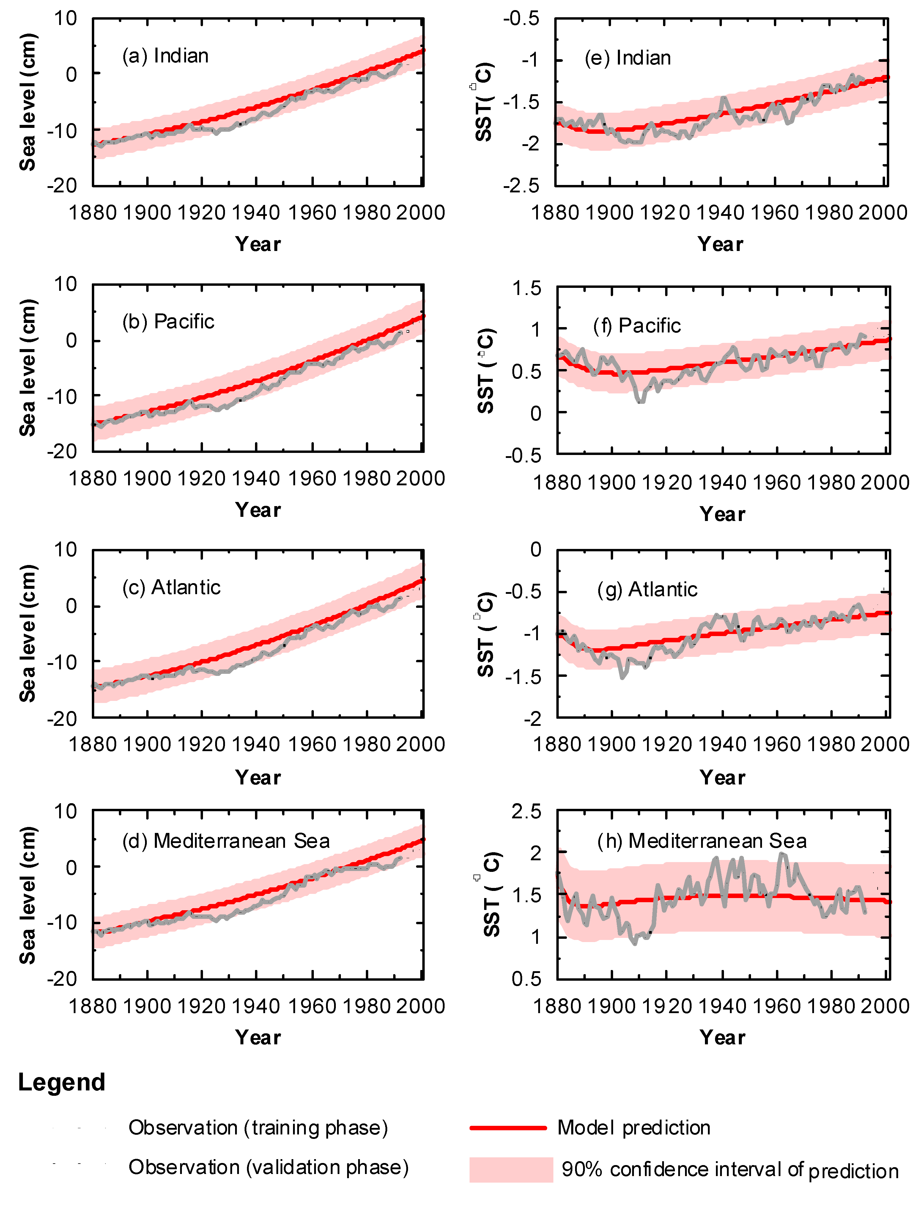
During model calibration, the ordinary least square method is applied to determine the model coefficients that minimize the absolute difference between the model results and the SST and sea level data. To evaluate the generalization ability of the proposed model, a cross-validation method is adopted, which uses part of the observational data (1880–2001) to calibrate the model and the rest of the data (1880–2001) to validate it over several periods of 10 years. This process is repeated at alternative intervals in the calibration stage within the period (1880–2001). The modeling results and 90% confidence intervals for model results were calculated following the methodology used in [26], as the full data is used in the final stage to obtain more accurate the calibration constants. The results obtained are shown in Figure 2, where one can see that outputs of the calibrated model agree with the historical records. The root-mean-square error (RMSE) of model fitting for the sea level of the Indian, Pacific, Atlantic Oceans and the Mediterranean Sea on average are 1.07 cm, 1.03 cm, 1.15 cm and 1.46 cm, respectively. The RMSE of model fitting for the SST of the Indian, Pacific, Atlantic Oceans and the Mediterranean Sea on average are 0.12 °C, 0.11 °C, 0.11 °C and 0.21 °C, respectively. In the validation phase, the RMSE of model fitting for the sea level of the Indian, Pacific, Atlantic Oceans and the Mediterranean Sea are, on average, 0.43 cm, 0.45 cm, 0.42 cm, and 0.48 cm, respectively, and the corresponding numbers for the regional mean SST’s are, on average, 0.05 °C, 0.1 °C, 0.15 °C and 0.29 °C, respectively. These statistics demonstrate that the proposed model is effective at representing the SLR and SSTs in three oceans and the Mediterranean Sea during the period 1880–2001. Notice that the relative deviation of model prediction from observation for SST is generally greater than that for the corresponding sea level. The difference in this deviation is a reflection of the greater temporal variability of SST data. Since the S-DSM approach adopted in this study aims to project SST and sea level over a long term (next century), the greater temporal variability does not constitute a significant influencing factor of the model results. It is interesting to note that the historical data for all oceans show an increasing trend for SLR and SSTs, except the SST of the Mediterranean Sea which is higher than the other three oceans, but almost flat for the period 1880–1992 as observed.
Coefficients of the calibrated model are given in Table 1. Based on these coefficients, the SST of each coastal region has a negative feedback on itself (the diagonal coefficients), and this negative feedback is larger than the influences of temperature changes of other regions, which indicates the mathematical stability of the increases that may be observed in predictive analysis. The highest negative feedback is observed for the Mediterranean Sea. It can also be observed that the Mediterranean Sea temperatures are influenced by the Atlantic Ocean and the Indian Ocean more than by the Pacific Ocean temperatures, as expected. The Atlantic Ocean temperature’s influence on the Mediterranean Sea is more than the Indian Ocean (of diagonal coefficients), which will create a cooling effect on the Mediterranean Sea. The interactions between sea levels of different regions are more complicated than those observed between temperatures. The sea level of Mediterranean Sea is influenced by the Indian and Atlantic Oceans the most (of diagonal terms). The Indian Ocean has a positive feedback which is higher than the Atlantic Ocean which has a negative feedback on Mediterranean Sea levels. The coefficients given in Table 1 can be directly used without the need of recalibration, and the ODEs can be solved numerically or analytically in other studies to obtain estimates of SLR and temperature change over the four oceans selected in this study, if needed.
4. Numerical Results and Discussion
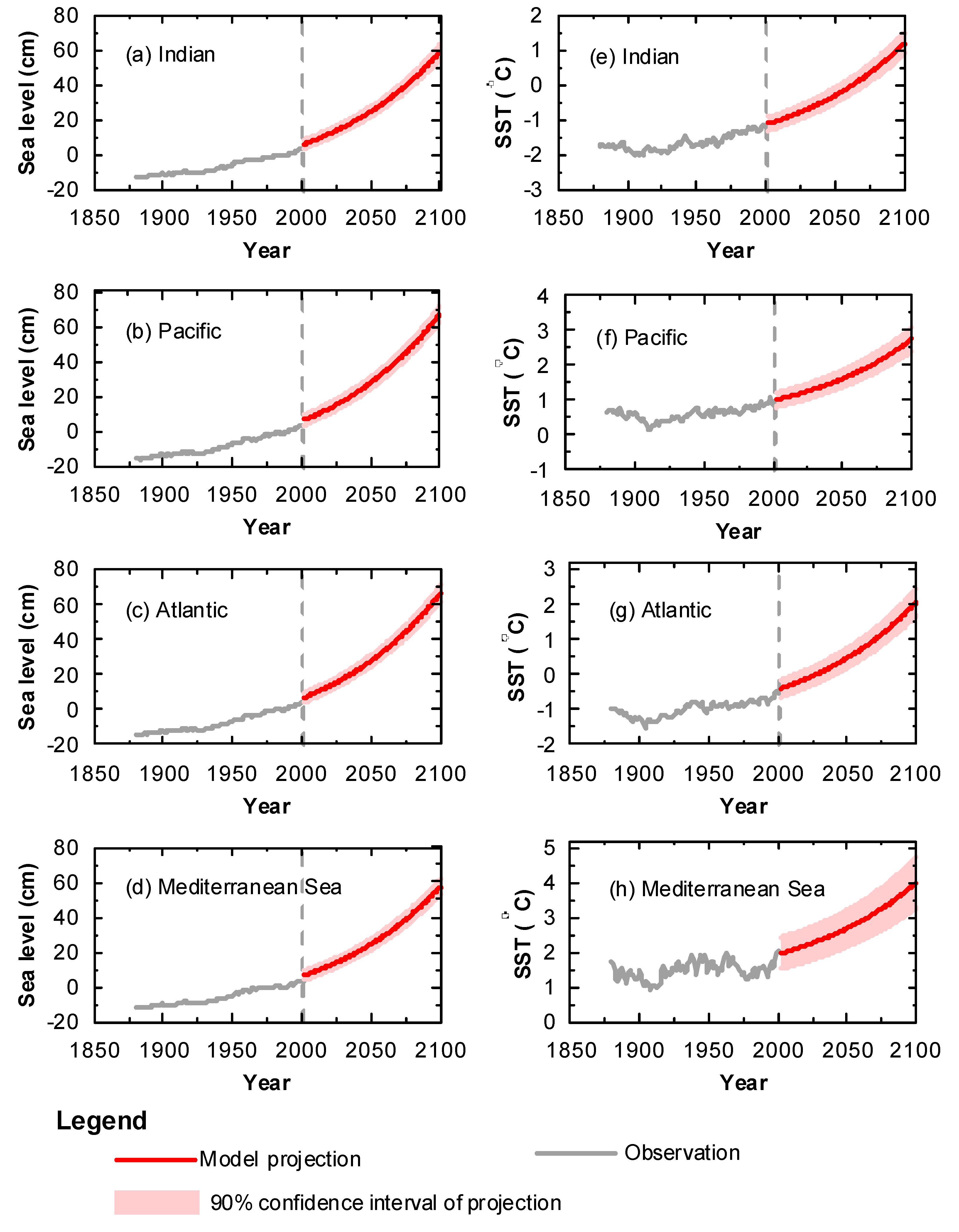
The spatial resolution of SLR due to climate change is analyzed using the S-DSM model, Equation (1). In this application the World’s oceans are divided into four, the Indian, Pacific and Atlantic Oceans and the Mediterranean Sea. Using the calibrated model coefficients, Table 1, the projected sea levels and SSTs in the 21st century are obtained as shown in Figure 3.
While the magnitude of SLR differs among the four regions, as shown in Figure 3, the overall sea level estimates of the World’s oceans are consistent with the global SLR results that are reported earlier in global analysis studies [7,26] and the Mediterranean Sea coastal data reported in [10]. In the Pacific and Atlantic Oceans, the sea levels are projected to reach 70 cm. In the Indian Ocean and the Mediterranean Sea, the sea levels will be below 60 cm relative to 1990 levels. The predicted difference of about 10 cm between the two pairs of oceans is a critical difference, which indicates that the inundation impact will be different between these coastlines. Since the sea mass in the Mediterranean Sea and the Indian Ocean is less than in the Atlantic and Pacific oceans, the steric effects due to temperature rise in the Mediterranean Sea and the Indian Ocean is less than that for the other two oceans, as expected. The Mediterranean Sea levels will follow the trend observed in the Indian Ocean more than the Atlantic Ocean. The trends observed in the SSTs show about 2–3 °C raise in SST relative to 1990 levels, with the highest increase of 3 °C observed for the Atlantic Ocean. Given that the temperatures are at about 2 °C in the Mediterranean Sea in the year 2000 relative to 1990 levels, this may create a critical temperature level in the Mediterranean Sea, since the temperatures may reach 4 °C in this region, again relative to 1990 levels. This will be the highest temperature observed among all four regions. The Indian Ocean will observe the lowest temperatures among the four at the end of the 21st century, reaching about 1 °C, relative to 1990 levels.
The SST and SLR analysis performed in [13] is the closest study in the literature that can be compared to the S-DSM analysis presented in this study. In [13], the authors have used the 1950–2000 data, similar to the data used in this paper, but analyzed the SLR only at the Mediterranean Sea based on steric effects using the temperature and salinity data at depth. Amplitudes and phases of the annual signal of temperature and salinity were averaged over the Mediterranean Sea similar to our analysis, and reported in their study. Their trend in the temperature data for the Mediterranean Sea is almost flat, with oscillations in amplitude as observed in the data used in this study. The predictions made for the period 2000–2001 for the temperature rise showed an increase of 2 to 4 °C, which is in excellent conformity with the predictions presented here. In [13], the authors predicted the East Mediterranean Sea to be warmer than the West Mediterranean Sea, which we cannot confirm in this study, since our results are for the Mediterranean Sea considered as a single region. Based on their analysis, the SLR changed significantly from the East to the West Mediterranean Sea, with the observed projected ranges from West to East being in the range −2 to 51 cm, which confirms the results reported in this study as the high-end values for the whole region. In [13], the thermosteric expansion in the Mediterranean Sea is reported to be comparable to that of the global ocean. In [13], since the hypothesis was based on mass balance and steric effects only for the Mediterranean Sea, the Eastern SLR in the Mediterranean Sea was compensated by lower sea levels in the Western Mediterranean Sea as a mass balance, which again we cannot confirm in our study. The hypothesis in this study is that the balance of the sea level is between Atlantic, Indian Oceans and the Mediterranean Sea, as opposed to looking for a mass balance only in the Mediterranean Sea. These are the basic differences in the hypothesis of the two studies. These comparisons between the two studies are very encouraging for the S-DSM results presented above. In [9,10,11,37] the local data obtained from multi-satellite altimetry and tide gauges were analyzed but projections were not made for the 21st century. Thus, comparison of their results with ours cannot be provided over the next century.
5. Conclusions
The S-DSM model is used to characterize spatial variations in SLR and SST for the Atlantic Ocean and Mediterranean Sea coastline of Europe. Given the hypothesis of S-DSM, the SLR and SSTs of remaining oceans were also reported. While matching the historical records well, the model predictions indicate that SLR and SST change behaviors of the Mediterranean Sea and the Atlantic Ocean coastline of Europe are going to be significantly different in the 21st century. According to the model predictions, from 2001 to 2100, mean SSTs of the Mediterranean Sea will rise to about 3–4 °C relative to 1990 levels, while that of the Atlantic Ocean will be approximately 1.5–2.5 °C higher than 1990 levels. This is a significant difference in predicted temperature levels, which gives a new meaning to the “Warm Waters” phrase that is historically used for the Mediterranean Sea. Contrary to the higher temperatures predicted for the Mediterranean Sea, the mean SLR in the Atlantic Ocean will be higher, reaching an approximately 70 cm rise relative to 1990 levels, while Mediterranean Sea levels will be below 60 cm, again relative to 1990 levels. This trend, as it is associated with the sea mass difference between the Atlantic Ocean and the Mediterranean Sea, also closely follows the year 2008 estimates that are reported in the literature, while using 14-year historical Mediterranean Sea temperature and sea level data [10,13,37].
According to the projections made in this study, inundation impacts on the Atlantic Ocean coastline of Europe will be more critical than the inundation impacts on the Mediterranean coastline. Contrary to this observation, with 3–4 °C higher temperatures predicted at the end of the 21st century relative to 1990 level, the high Mediterranean Sea temperatures will impact the biodiversity of the Mediterranean Sea significantly. It is clear that this would be a more important problem to tackle for the Mediterranean Sea than the inundation problem at the coastline of the Mediterranean Sea. As presented in this study a more refined spatial model of SLR and temperature estimates may provide critical contributions to inundation and biodiversity health assessment issues of the oceans surrounding the European coastline while providing baseline databases for subsequent formulation of management policies.
Acknowledgments
The first author would like to express his sincere appreciation to Orhan Uzun (Rector, Bartın University) for his support in providing the accommodations necessary for him to work on this paper while visiting Bartın University, Turkey.
Author Contributions
In the preparation of this article, the first author Mustafa M. Aral contributed to the development of the concept and the analysis procedures used in the methodology. The second author, Biao Chang contributed to the computational aspects of the study. Both authors have contributed to the writing and proof reading the manuscript.
Conflicts of Interest
The authors declare no conflict of interest. This study was not funded by funding agencies.
References
- Brown, S.; Nicholls, R.J.; Lowe, J.A.; Hinkel, J. Spatial variations of sea-level rise and impacts: An application of DIVA. Clim. Chang. 2016, 134, 403–416. [Google Scholar] [CrossRef]
- Chang, B.; Guan, J.; Aral, M.M. Modeling spatial variations of sea level rise and corresponding inundation impacts: A case study for Florida, USA. J. Water Qual. Expo. Health 2013, 6, 39–51. [Google Scholar] [CrossRef]
- Meehl, G.A.; Stocker, T.F.; Friedlingstein, W.D.; Collins, P.; Gaye, A.T.; Gregory, J.M.; Kitoh, A.; Knutti, R.; Murphy, J.M.; Noda, A.; et al. Projections of global average sea level change for the 21st century. In Climate Change 2007: The Physical Science Basis. Contribution of Working Group I to the Fourth Assessment Report of the Intergovernmental Panel on Climate Change; Solomon, S., Qin, D., Manning, M., Chen, Z., Marquis, M., Averyt, K.B., Tignor, M., Miller, H.L., Eds.; Cambridge University Press: Cambridge, UK; New York, NY, USA, 2007. [Google Scholar]
- Neil, J.W.; Ivan, D.H.; John, A.C.; Terry, K.; Christopher, S.W.; Tim, R.P.; Phil, J.W.; Reed, J.B.; Kathleen, L.M.; Zai-Jin, Y.; et al. Australian sea levels—Trends, regional variability and influencing factors. Earth Sci. Rev. 2014, 136, 155–174. [Google Scholar]
- Nicholls, R.J.; Wong, P.P.; Burkett, V.; Codignotto, J.; Hay, J.; McLean, R.; Ragoonaden, S.; Woodroffe, C.D.; Abuodha, P.A.O.; Arblaster, J. Coastal systems and low-lying areas. In Climate Change 2007: Impacts, Adaptation and Vulnerability. Contribution of Working Group II to the Fourth Assessment Report of the Intergovernmental Panel on Climate Change; Parry, M.L., Canziani, O.F., Palutikof, J.P., van der Linden, P., Hanson, C.E., Eds.; Cambridge University Press: Cambridge, UK; New York, NY, USA, 2007; pp. 316–357. [Google Scholar]
- Asbury, H.S.; Kara, S.D.; Peter, A.H. Hotspot of accelerated sea-level rise on the Atlantic coast of North America. Nat. Clim. Chang. Lett. 2012, 2, 884–888. [Google Scholar] [CrossRef]
- Intergovernmental Panel on Climate Change. Summary for Policymakers. Available online: http://www.ipcc.ch/report/ar5/wg1/ (accessed on 26 January 2017).
- Rosenzweig, C.; Solecki, W. New York City Panel on Climate Change, Climate Risk Information: Observations, Climate Change Projections, and Maps; Prepared for use by the City of New York Special Initiative on Rebuilding and Resiliancy; Rosenzweig, C., Solecki, W., Eds.; New York City Panel on Climate Change (NPCC2): New York, NY, USA, 2013. [Google Scholar]
- Cazenavea, A.; Bonnefond, P.; Merciera, F.; Dominha, K.; Toumazoua, V. Sea level variations in the Mediterranean Sea and Black Sea from satellite altimetry and tide gauges. Glob. Planet. Chang. 2002, 34, 59–86. [Google Scholar] [CrossRef]
- Criado-Aldeanueva, F.; Vera, J.D.R.; García-Lafuente, J. Steric and mass-induced Mediterranean Sea level trends from 14 years of altimetry data. Glob. Planet. Chang. 2008, 60, 563–575. [Google Scholar] [CrossRef]
- Le Cozannet, G.; Garcin, M.; Yates, M.; Idier, D.; Meyssignac, B. Approaches to evaluate the recent impacts of sea-level rise on shoreline changes. Earth Sci. Rev. 2014, 138, 47–60. [Google Scholar] [CrossRef]
- Lichter, M.; Felsenstein, D. Asessing the costs of sea-level rise and extreme flooding at the local level: A GIS-based approach. Ocean Coast Manag. 2012, 59, 47–62. [Google Scholar] [CrossRef]
- Marta, M.; Michael, N.T. Comparison of results of AOGCMs in the Mediterranean Sea during the 21st century. J. Geophys. Res. 2008, 113. [Google Scholar] [CrossRef]
- Cabanes, C.; Huck, T.; Verdiere, A. Contribution of wind forcing and surface heating to interannual sea level variations in the Atlantic Ocean. J. Phys. Oceanogr. 2006, 36, 1739–1750. [Google Scholar] [CrossRef]
- Mitrovica, J.X.; Gomez, N.; Clark, P.U. The sea-level fingerprint of west antarctic collapse. Science 2009, 323, 753. [Google Scholar] [CrossRef] [PubMed]
- Pardaens, A.K.; Lowe, J.A.; Brown, S.; Nicholls, R.J.; de Gusmao, D. Sea-level rise and impacts projections under a future scenario with large greenhouse gas emission reductions. Geophys. Res. Lett. 2011, 38, L12604. [Google Scholar] [CrossRef]
- Wunsch, C.; Ponte, R.M.; Heimbach, P. Decadal trends in sea level patterns: 1993–2004. J. Clim. 2007, 20, 5889–5911. [Google Scholar] [CrossRef]
- Etkins, R.; Epstein, E.S. The rise of global mean sea-level as an indication of climate change. Science 1982, 215, 287–289. [Google Scholar] [CrossRef] [PubMed]
- Gornitz, V.L.; Lebedeff, S.; Hansen, J. Global sea-level trend in the past century. Science 1982, 215, 1611–1614. [Google Scholar] [CrossRef] [PubMed]
- Rahmstorf, S. A semi-empirical approach to projecting future sea-level rise. Science 2007, 315, 368–370. [Google Scholar] [CrossRef] [PubMed]
- Holgate, S.; Jevrejeva, S.; Woodworth, P.; Brewer, S. Comment on “A semi-emprical approach to projecting future sea-level rise”. Science 2007, 317, 1866. [Google Scholar]
- Vermeer, M.; Rahmstorf, S. Global sea level linked to global temperature. Proc. Natl. Acad. Sci. USA 2009, 106, 21527–21532. [Google Scholar] [CrossRef] [PubMed]
- Grinsted, A.; Moore, J.C.; Jevrejeva, S. Reconstructing sea level from paleo and projected temperatures 200 to 2100 AD. Clim. Dyn. 2010, 34, 461–472. [Google Scholar] [CrossRef]
- Jevrejeva, S.; Grinsted, A.; Moore, J.C. Anthropogenic forcing dominates sea level rise since 1850. Geophys. Res. Lett. 2009, 36, L20706. [Google Scholar] [CrossRef]
- Jevrejeva, S.; Moore, J.C.; Grinsted, A. How will sea level response to changes in natural and anthropogenic forcings by 2100? Geophys. Res. Lett. 2010, 37, L07703. [Google Scholar]
- Aral, M.M.; Guan, J.; Chang, B. A dynamic system model to predict global sea-level rise and temperature change. J. Hydrol. Eng. 2012, 17, 237–242. [Google Scholar] [CrossRef]
- Guan, J.; Chang, B.; Aral, M.M. A Dynamic Control System Model for Global Temperature Change and Sea level Rise in Response to CO2 Emissions. Clim. Res. 2013, 58, 55–66. [Google Scholar] [CrossRef]
- Aral, M.M. Perspectives and Challenges on Climate Change and Its Effects on Water Quality and Health. Water Qual. Expo. Health 2014, 6, 1–5. [Google Scholar] [CrossRef]
- Aral, M.M.; Guan, J. Global Sea Surface Temperature and Sea Level Rise Estimation with Optimal Historical Time Lag Data. Water 2016, 8. [Google Scholar] [CrossRef]
- Schmith, T.; Johansen, S.; Thejll, P. Statistical analysis of global surface temperature and sea level using cointegration methods. J. Clim. 2012, 25, 7822–7833. [Google Scholar] [CrossRef]
- Wu, Q.; Luu, Q.-H.; Tkalich, P.; Chen, G. An improved empirical dynamic control system model of global mean sea level rise and surface temperature change. Theor. Appl. Climatol. 2017. [Google Scholar] [CrossRef]
- Chang, B.; Guan, J.; Aral, M.M. Scientific Discourse: Climate Change and Sea-Level Rise. J. Hydrol. Eng. ASCE 2015, 20, A4014003-1-14. [Google Scholar] [CrossRef]
- Commonwealth Scientific and Industrial Research Organisation (CSIRO) Sea Level Data. 2011. Available online: http://www.cmar.csiro.au/sealevel/sl_data_cmar.html (accessed on 8 April 2017).
- Church, J.A.; White, N.J.; Coleman, R.; Lambeck, K.; Mitrovica, J.X. Estimates of the regional distribution of sea level rise over the 1950–2000 period. J. Clim. 2004, 17, 2609–2625. [Google Scholar] [CrossRef]
- Pham, D. Spatial models for fuzzy clustering. Comput. Vis. Image Underst. 2001, 84, 285–297. [Google Scholar] [CrossRef]
- Smith, T.M.; Reynolds, R.W.; Peterson, T.C.; Lawrimore, J. Improvements to NOAA’s historical merged land-ocean surface temperature analysis (1880–2006). J Clim. 2008, 21, 2283–2296. [Google Scholar] [CrossRef]
- Feneglio-Marc, L. Long-term sea level change in the Mediterranean Sea from multi-satellite altimetry and tide gauges. Phys. Chem. Earth 2002, 27, 1419–1431. [Google Scholar] [CrossRef]
Figure 1.
Approximate Ocean regions used in the four region S-DSM model.
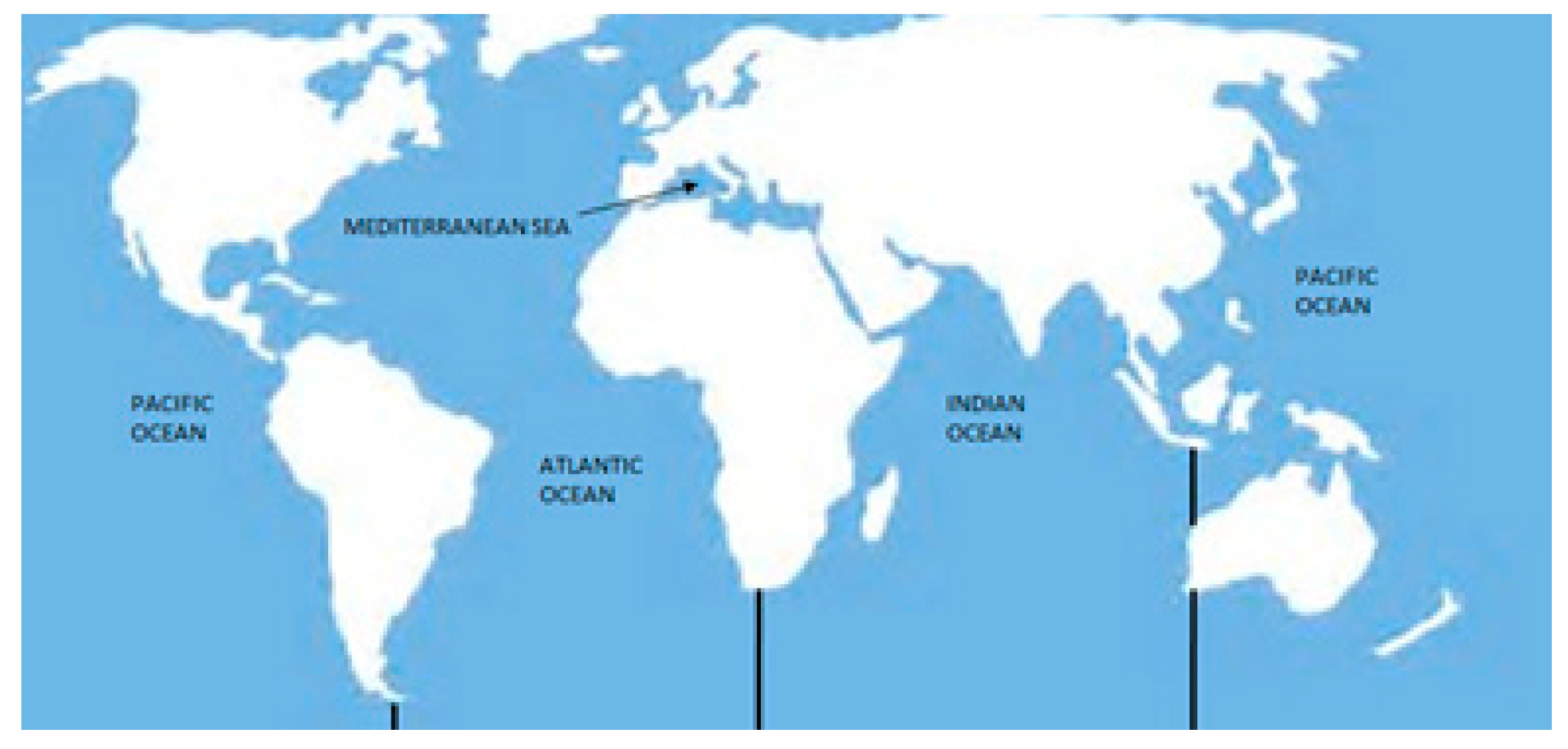
Figure 2.
Four region model results in the calibration phase (solid black lines represent the historical data).
Figure 2.
Four region model results in the calibration phase (solid black lines represent the historical data).

Figure 3.
Sea level projections for the four regions of the World’s Oceans.


Table 1.
Four Region Model coefficient matrices.
| Rate of Rise | Contributing Variable | ||||||||
|---|---|---|---|---|---|---|---|---|---|
| H | T | Constant | |||||||
| dH/dt | A (year−1) | B (cm/°C/year) | CH (cm/year) | ||||||
| −0.69 | 0.60 | −0.08 | 0.10 | −0.07 | 0.25 | 0.34 | −0.24 | 0.76 | |
| −0.45 | 0.47 | −0.16 | 0.08 | 0.06 | 0.19 | 0.38 | −0.25 | 0.96 | |
| −1.07 | 0.83 | −0.04 | 0.16 | −0.12 | 0.35 | 0.35 | −0.29 | 0.81 | |
| 2.02 | −0.53 | −1.08 | −0.19 | 0.16 | 0.11 | 0.06 | −0.21 | 0.24 | |
| dT/dt | D (°C/cm/year) | E (year−1) | CT (°C/year) | ||||||
| −0.38 | 0.15 | 0.18 | 0.01 | −0.26 | 0.01 | 0.09 | 0.01 | −0.18 | |
| 0.09 | −0.05 | −0.02 | −0.01 | 0.17 | −0.21 | −0.07 | 0.07 | 0.23 | |
| −0.37 | 0.20 | 0.11 | 0.02 | −0.04 | 0.04 | −0.18 | 0.06 | −0.20 | |
| 0.47 | −0.06 | −0.36 | 0.01 | 0.13 | −0.03 | 0.20 | −0.34 | 0.78 | |
© 2017 by the authors. Licensee MDPI, Basel, Switzerland. This article is an open access article distributed under the terms and conditions of the Creative Commons Attribution (CC BY) license (http://creativecommons.org/licenses/by/4.0/).
Share and Cite
MDPI and ACS Style
Aral, M.M.; Chang, B. Spatial Variation of Sea Level Rise at Atlantic and Mediterranean Coastline of Europe. Water 2017, 9, 522. https://doi.org/10.3390/w9070522
AMA Style
Aral MM, Chang B. Spatial Variation of Sea Level Rise at Atlantic and Mediterranean Coastline of Europe. Water. 2017; 9(7):522. https://doi.org/10.3390/w9070522
Chicago/Turabian StyleAral, Mustafa M., and Biao Chang. 2017. "Spatial Variation of Sea Level Rise at Atlantic and Mediterranean Coastline of Europe" Water 9, no. 7: 522. https://doi.org/10.3390/w9070522
Note that from the first issue of 2016, this journal uses article numbers instead of page numbers. See further details here.