River Stage Modeling by Combining Maximal Overlap Discrete Wavelet Transform, Support Vector Machines and Genetic Algorithm


Department of Constructional and Environmental Engineering, Kyungpook National University, Sangju 37224, Korea;
*
Author to whom correspondence should be addressed.
Water 2017, 9(7), 525; https://doi.org/10.3390/w9070525
Submission received: 21 May 2017
/
Revised: 3 July 2017
/
Accepted: 5 July 2017
/
Published: 15 July 2017
Abstract
:This paper proposes a river stage modeling approach combining maximal overlap discrete wavelet transform (MODWT), support vector machines (SVMs) and genetic algorithm (GA). The MODWT decomposes original river stage time series into sub-time series (detail and approximation components). The SVM computes daily river stage values using the decomposed sub-time series. The GA searches for the optimal hyperparameters of SVM. The performance of MODWT–SVM models is evaluated using efficiency and effectiveness indices; and compared with that of a single model (multilayer perceptron (MLP) and SVM), discrete wavelet transform (DWT)-based models (DWT–MLP and DWT–SVM) and MODWT–MLP models. The conjunction of MODWT, SVM and GA improves the performance of the SVM model and outperforms the single models. The MODWT–based models using the SVM model enhance model performance and accuracy compared to those of using MLP model. Also, hybrid models coupling MODWT, SVM and GA improve model performance and accuracy in daily river stage modeling as compared with those combined with DWT. The MODWT–SVM model using the Coiflet 12 (c12) mother wavelet, MODWT–SVM-c12, produces the best efficiency and effectiveness among all models. Therefore, the conjunction of MODWT, SVM and GA can be an efficient and effective approach for modeling daily river stages.
1. Introduction
Modeling the nonlinear behavior of hydrological variables accurately is essential for effective water resource management including water supply, reservoir operation, drought forecasting, flood damage reduction and aquatic ecosystem conservation in South Korea. Soft computing approaches such as artificial neural networks (ANNs), support vector machines (SVMs) and adaptive neuro-fuzzy inference system (ANFIS) have been widely applied for modeling complex nonlinear hydrological relationships including precipitation, streamflow, rainfall-runoff, evaporation and groundwater [1,2,3,4,5,6,7,8,9].
Recently, hybrid time series modeling approaches utilizing wavelet transform have been one of the research themes studied actively in the hydrological field [8,9,10,11,12,13,14]. In terms of signal analysis, the wavelet transform is a signal decomposition method which splits an original signal into sub-signals, including detail and approximation (smooth) components. Adamowski and Sun [10] suggested a hybrid model combining discrete wavelet transform (DWT) and ANN for streamflow forecasting. Kisi et al. [11] predicted short- and long-term air temperatures using wavelet-based genetic programming. Okkan and Serbes [12] modeled reservoir inflow using a combination of DWT and black box models including ANNs, multiple linear regression and least square support vector machines (LS-SVMs). Raghavendra and Deka [14] proposed a combined model of wavelet packet transform (WPT) and SVM for groundwater level prediction. Seo et al. [8] developed two hybrid water level forecasting models, including DWT-based ANN (WANN) and DWT-based ANFIS (WANIFS). Seo et al. [9] developed three hybrid river stage forecasting models, including WPT-based ANN (WPANN), WPT-based ANFIS (WPANFIS) and WPT-based SVM (WPSVM).
Several methods can be used for decomposing a signal. Time windowing and Fourier analysis methods have provided the temporal and frequency decompositions of a signal, respectively. Both methods lack the ability to extract the signal components for multiple time scales [15]. Furthermore, the time windowing method requires the selection of an appropriate averaging time. The Fourier analysis method may require preprocessing including tapering, data windowing, detrending and mean subtraction [15]. Unlike the time windowing and Fourier analysis methods, DWT decomposes a signal in time and frequency domains, and provides the effective extraction of signal components for multiple time scales. However, DWT also has drawbacks such as signal length restriction and lack of translation-invariance [15]. DWT is limited to a signal length that is a power-of-two multiple. The power-of-two restriction on signal length should be relaxed for applying the DWT. The signal decomposition by the DWT depends on whether an event spans or is within a wavelet averaging window. It is also sensitive to the starting position of the signal [15]. Like the DWT, the maximal overlap discrete wavelet transform (MODWT) decomposes a signal in the time and frequency domains. However, the MODWT keeps down-sampled values at each decomposition level, whereas the DWT discards the values. There is no need to relax the power-of-two restriction for applying the MODWT. In other words, the MODWT can be applied for all signal lengths [15]. In addition, the MODWT provides several merits over the DWT. Further details on them can be found in Cornish and Percival [15]. Therefore, the advantages of MODWT over other methods suggest that the conjunction of MODWT and soft computing models may be a more effective and efficient approach for river stage modeling.
This study proposes the coupling of MODWT, SVM and genetic algorithm (GA) for daily river stage modeling. MODWT and SVM are adopted for decomposing an original signal and estimating the river stage, respectively. The GA is applied for searching the optimal hyperparameters of the SVM. For investigating the model performance (efficiency and effectiveness), a case study was conducted for daily river stage modeling in the Chogang Watershed, South Korea. The model performance is assessed based on statistical indices (efficiency and effectiveness indices) and graphical comparison. The performances of the MODWT–SVM models are compared with those of the single models (multilayer perceptron (MLP) and SVM), DWT-based models (DWT–MLP and DWT–SVM) and MODWT–MLP models.
2. Materials and Methods
2.1. Data Used
The Chogang Watershed in South Korea was chosen for applying the DWT- and MODWT-based river stage modeling approaches. The watershed is a tributary of the Geum River, which has the third largest river basin in South Korea. As depicted in Figure 1, the study area is a mountainous watershed located in the eastern region of the Geum River Basin. The watershed area is 664.62 km2, the stream length is 63.18 km, the average watershed elevation is 369.18 m, and the average watershed slope is 39.94% (http://www.wamis.go.kr, accessed on 19 May 2017).
Daily river stage data for four streamflow gauging stations were collected from the Water Management Information System (WAMIS) (http://www.wamis.go.kr, accessed on 19 May 2017). The WAMIS is a portal information system for providing various information on the water resources of South Korea. As seen in Figure 1, the gauging stations include Simcheon, Songcheon, Baekhwagyo and Hwanggan. The data for the period of 2008–2016 were prepared for river stage modeling. The data were partitioned into training (2008–2013) and testing datasets (2014–2016) on a yearly basis, and also into low (), medium () and high stages () groups [16], where is the river stage value, and and are the mean and standard deviation of the river stage time series.
2.2. Discrete Wavelet Transform (DWT)
DWT, which is a simpler version of continuous wavelet transform, is a multiresolution analysis (MRA) technique which decomposes an original signal into approximation and detail components. This section outlines the basic concept of DWT. Detailed information on the DWT can be found in Nason [17]. According to Mallat [18], DWT can be written as the following equation [10]:
where j and k are integer values controlling wavelet scale and translation; is the fixed scale step (commonly ); is the mother wavelet; and is the location parameter (commonly ). For a discrete signal , the DWT computes the wavelet coefficient for the discrete wavelet of scale and location using the following equation [16]:
where is the wavelet coefficient and N = an integer power of two.
Mallat’s algorithm [18] is generally applied for the practical implementation of DWT. The algorithm uses low- and high-pass filters instead of wavelets. Figure 2 shows a flowchartfor three-level DWT. As seen in Figure 2, an original signal is decomposed into detail components (D1, D2 and D3) and an approximation component (A3) using the algorithm. The filters are determined depending on the mother wavelets which are selected in advance. The mother wavelets include Daubechies wavelet (Daublet), Daubechies’ least-asymmetric wavelet (Symmlet), Coiflet, Morlet (Gabor wavelet), Meyer wavelet, and Shannon wavlets (Littlewood–Paley wavelet), and so on. Details on different wavelets can be found in Percival and Walden [19] and Nason [17]. For decomposing input signals using wavelet analysis, the decomposition level should be determined beforehand. The level L was determined based on Equation (3) [20]:
where int[·] is the function that returns the nearest integer of a number and n is the data length.
2.3. Maximal Overlap Discrete Wavelet Transform (MODWT)
MODWT is a mathematical technique which transforms a signal into multilevel wavelet and scaling coefficients. MODWT has several merits in comparison with DWT as discussed in Cornish et al. [15]. For example, MODWT can be properly defined for arbitrary signal length, while the DWT is limited to a signal length with an integer multiple of a power of two. This section outlines the concept of MODWT. Details on MODWT can be found in Percival and Walden [19].
For a discrete signal , the elements of the jth level MODWT wavelet and scaling coefficients, and , can be written as Equations (4) and (5), respectively [19]:
where is the tth element of the jth level MODWT wavelet coefficient; is the tth element of the jth level MODWT scaling coefficient; and are the jth level MODWT high- and low-pass filters (wavelet and scaling filters) yielded by periodizing and to length n, respectively; and are the jth level MODWT high-pass filter () and low-pass filter (); and are the jth level DWT high- and low-pass filters; and L is the highest decomposition level. The filters are determined depending on the mother wavelets, as in DWT.
Figure 3 shows a flowchart for three-level MODWT. As seen in Figure 3, the MODWT-based MRA decomposes an original signal into a low-pass filtered approximation component (A3) and high-pass filtered detail components (D1, D2 and D3). The MODWT-based MRA can be written as Equations (6)–(8) [19];
where is the approximation component and is the detail components ().
2.4. Multilayer Perceptron (MLP)
ANN is a multilayered computing system for modeling complex nonlinear and multi-dimensional relationships. MLP, which is the most commonly applied ANN structure, consists of several layers. For hydrological applications, MLP with three layers, including input, output and hidden layers, is typically used, as shown from Figure 4. As described in Günther and Fritsch [21], three-layered MLP with J hidden nodes calculates Equation (9):
where is the input vector; f is the activation function; is the output vector; is the intercept for output node; is the connection weight; is the connection weight vector; and is the intercept for the jth hidden node. Details on the MLP are given in Günther and Fritsch [21].
For MLP modeling, the number of hidden nodes and the type of activation function should be determined in advance. The optimal number of hidden nodes can be determined utilizing trial-and-error or optimization methods. The activation functions used in the MLP include logistic sigmoid, linear and hyperbolic tangent functions. Although the activation functions depend on the type of network and training algorithm, the logistic sigmoid activation function is often employed since it is real-valued, continuous, differentiable and computationally easy to perform. Furthermore, the logistic sigmoid activation function is often used to introduce nonlinear behavior in the MLP [21].
2.5. Support Vector Machine (SVM)
The SVM, which is a class of statistical models developed by Vapnik [22], is a supervised machine learning model for solving classification and regression problems. In a SVM, a nonlinear mapping function maps original data into a high-dimensional space. This section outlines the basic concept of SVM. Details on the SVM can found in Vapnik [22] and Noori et al. [23]. Given a training dataset , where is the input vector of m component and is the target value, the SVM for regression can be formulated as Equation (10) [22]:
where is the weight vector; is the mapping function; and b is the bias.
The parameters, and b, are estimated by minimizing Equation (11) [22]:
where is the regularized risk function; C is the regularization parameter; and is the -insensitive loss function. The function can be written as Equation (12) [22]:
where is the parameter of insensitive loss function. The hyperparameters, C and , should be determined beforehand. Thus, the SVM conducts linear regression in the high-dimensional space utilizing the -insensitive loss function. By introducing the non-negative slack variables and , the is converted into the optimization problem as in Equation (13) [22]:
By introducing the dual set of Lagrange multipliers, and , the SVM can be written as follows [22]:
Thus, the non-linear regression function of SVM can be expressed as Equation (15) [22]:
where is the support vector; m is the number of support vectors; and is the kernel function. Figure 5 shows a three-layer SVM model architecture with eight inputs and one output. The radial basis function (RBF), which is suitable for regression problems, was used in this study. The function can be written as Equation (16) [22]:
where is the kernel parameter () and p is the width parameter.
For SVM modeling, the optimal hyperparameters, including regularization, insensitive loss function and kernel parameters, should be selected in advance. Since the hyperparameters are difficult to determine by a trial-and-error approach, the optimal hyperparameters are usually selected utilizing optimization algorithms.
2.6. Genetic Algotrithm (GA)
GA, which is a class of evolutionary algorithms, is a stochastic optimization algorithm based on evolution strategy. GAs have been successfully applied to search for approximate or exact solutions to optimization problems [24]. A GA was applied to search the optimal hyperparameters of SVM in this study. The main genetic operators consist of selection, crossover and mutation operators. The selection operator chooses excellent chromosomes (set of candidate parameters), which are also called individuals, to be reproduced. The crossover operator exchanges genes (candidate parameters) between two chromosomes. The mutation operator determines whether a chromosome mutates to the next generation or not. The crossover and mutation operators generate new offspring and population (set of all parameters) in the next generation. The evolution process can be summarized as follows [25]:
- Step 1. Generate an initial random population .
- Step 2. Compute the fitness of each chromosome in the population, and assign probability typically proportional to the fitness.
- Step 3. Reproduce new population using selection, crossover and mutation operators.
- Step 4. Repeat from step 2 to step 3 until stop conditions are met. The algorithm yields as the optimum.
For applying the GA optimization, the tuning parameters should be set in advance. The main tuning parameters include population size, number of generations, elite count, and crossover and mutation rates. The population size is the number of chromosomes in population (typically, population size = 20–100). The number of generations is related to the improvement in the fitness function. The crossover rate is the probability that crossover will occur between chromosomes (typically, crossover rate = 0.80–0.95). The mutation rate is the probability that a mutation will occur in a parent chromosome (typically, mutation rate = 0.5–1.0) [25,26]. The elite count is the number of best fitness individuals to survive at each generation, which can be computed using the following equation [25]:
where popSize is the population size and int(·) is the function which returns integer part.
2.7. River Stage Modeling Using DWT and MODWT
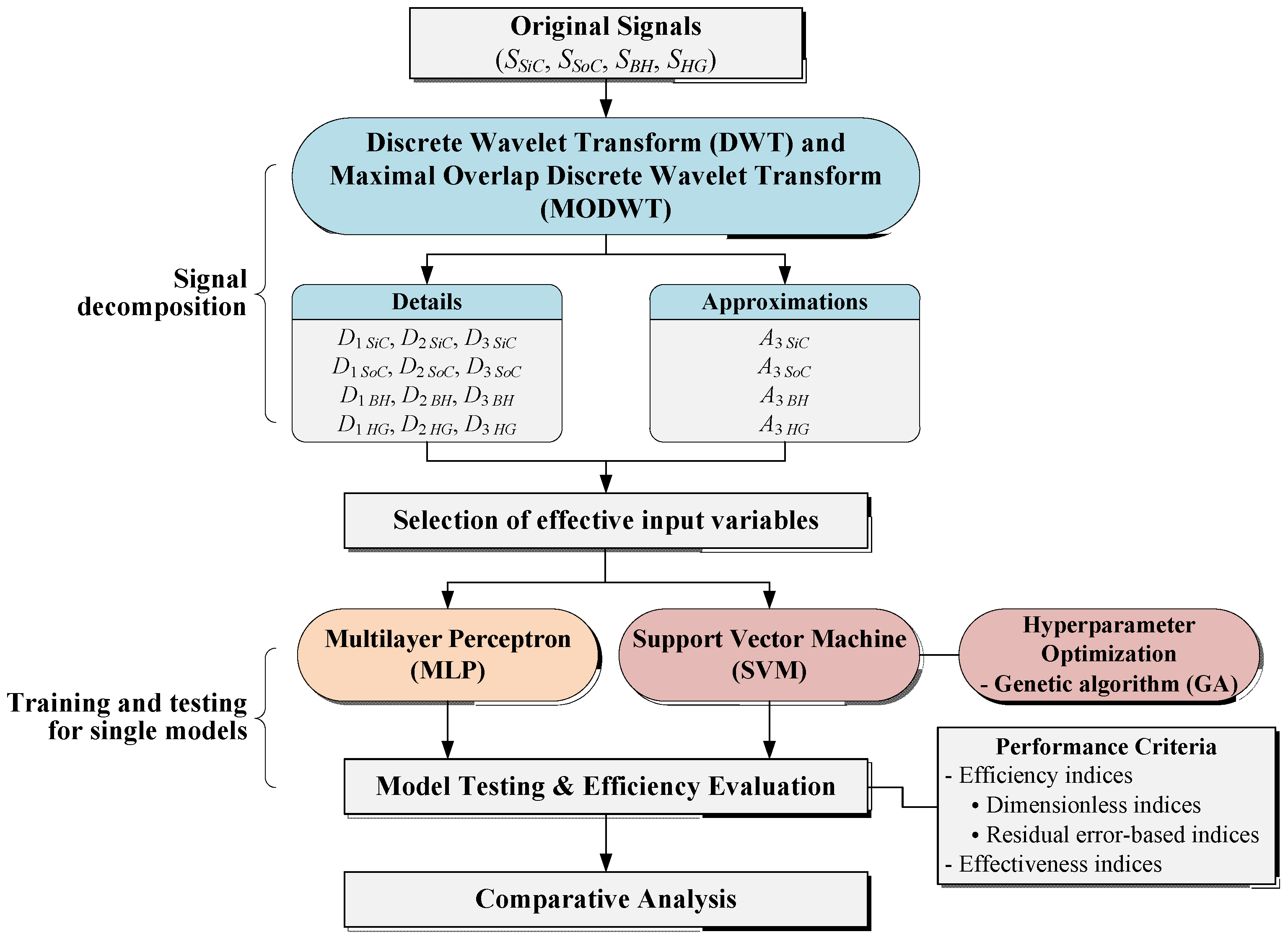
In river stage modeling using DWT and MODWT, the DWT and MODWT decompose original input signals (daily river stage data) into sub-signals (detail and approximation components). The sub-signals are then used as the inputs of single models, MLP and SVM. As depicted in Figure 6, the DWT- and MODWT-based river stage modeling approaches are comprised of a three-step algorithm. The algorithm is outlined as follows:
- Step 1. Decompose original input signals into sub-signals (detail and approximation components) utilizing DWT and MODWT.
- Step 2. Select effective inputs among the sub-signals.
- Step 3. Train and test single models, MLP and SVM, utilizing the effective inputs.
2.8. Model Efficiency Evaluation
The efficiencies of single, DWT- and MODWT-based river stage modeling approaches were assessed utilizing dimensionless and residual error-based indices (see Appendix A).
- -
- Dimensionless indices: coefficient of efficiency (CE), index of agreement (d) and coefficient of determination (r2)
- -
- Residual error-based indices: root-mean-square error (RMSE), mean absolute error (MAE), mean squared relative error (MSRE) and mean higher order error (MS4E)
The CE, d and r2 provide the measures of correlation between the estimated and observed data. The CE measures the capability of the model which estimates stage values different from the mean stage. The r2 measures the variability of observed stage which is explained by a model. The d measures overall agreement between the estimated and observed data. The RMSE and MS4E measure goodness of fit at high stages, whereas the MSRE measures it at moderate stages. The MAE measures overall agreement between the estimated and observed data [27,28]. Higher dimensionless and lower residual error-based indices indicate whether a model produces superior efficiency to other models. Details on the indices can be found in Dawson and Wilby [27].
2.9. Model Effectiveness Evaluation
The effectiveness of single, DWT- and MODWT-based river stage modeling approaches are assessed utilizing average absolute relative error (AARE) and threshold statistics (TS) (see Appendix B). AARE and TS evaluate model effectiveness by measuring the predictive ability of a model. Furthermore, AARE and TS provide a more appropriate assessment since they give appropriate weight on all magnitude flows [29,30,31,32]. Lower AARE and higher TS values indicate that a model produces superior effectiveness to other models.
3. Results and Discussion
3.1. Model Development
One of the most important steps for developing single, DWT- and MODWT-based models is to select effective inputs. In this study, the optimal lags of inputs were determined based on average mutual information (AMI), autocorrelation function (ACF), partial autocorrelation function (PACF) and cross correlation function (CCF) [33,34]. The optimal lag for the river stage series of the Simcheon gauging station can be defined as a lag value at which the ACF, PACF and AMI show significant correlation. Specifically, the optimal lag is determined when the ACF reaches zero or a small value, or the PACF decays within the confidence interval, or the AMI attains the first minimum [33,34]. The optimal lags for other gauging stations were determined as lag values at which the CCFs between Simcheon and other gauging stations showed significant correlation, respectively. Based on the methods, the optimal lags were determined as lag 6 for Simcheon and lag 1 for the other gauging stations (Songcheon, Baekhwagyo and Hwanggan). Table 1 summarizes the input combination for developing the models.
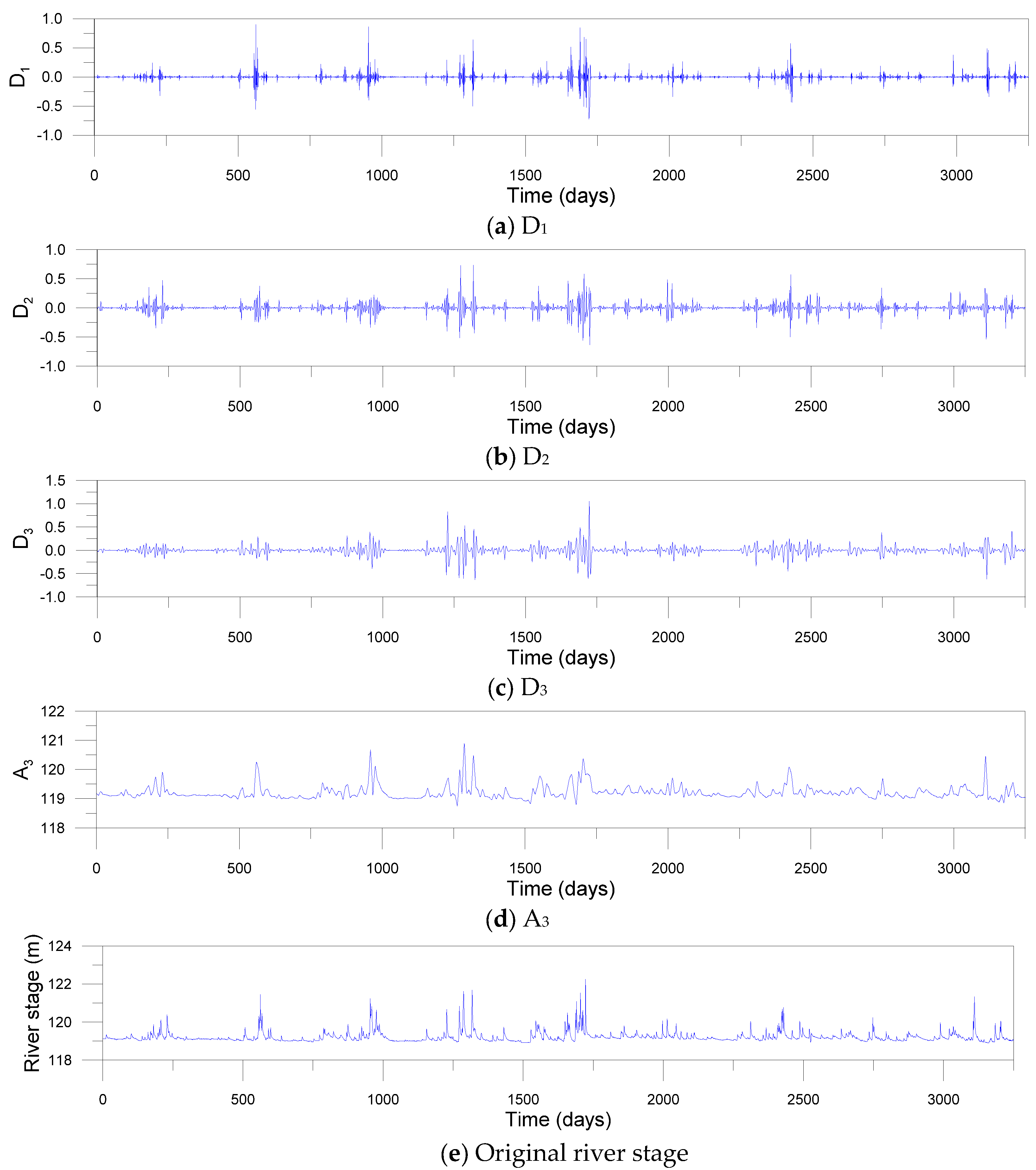
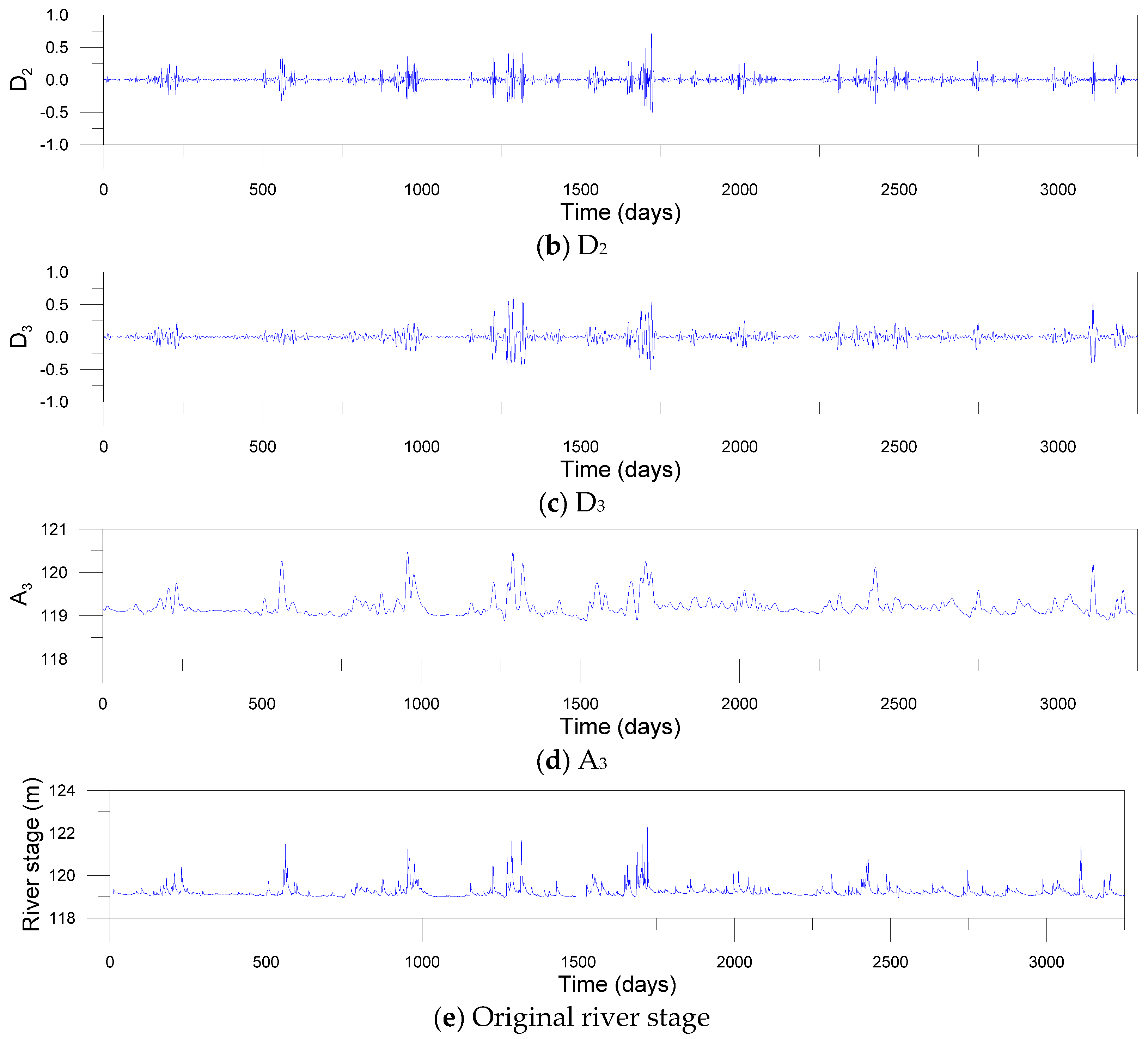
For the decomposing of input signals using DWT and MODWT, the decomposition level should be determined beforehand. In this study, the level L = 3 was determined based on Equation (3). Mother wavelets should be also selected ahead of time. Since the accuracy of DWT- and MODWT-based models depends on mother wavelets, nine mother wavelets were used, including Daublets (d6, d12 and d18), Symmlets (s6, s12 and s18) and Coiflets (c6, c12 and c18). The Daublet, also called Daubechies wavelet, is a collection of orthogonal wavelets with compact support. The Symmlet, also called least-asymmetric wavelet, is a modified version of Daublet which is proposed to enhance symmetry. The Symmlet is an orthogonal, continuous, compactly supported, but nearly symmetric wavelet. The Coiflet, also called Coifman wavelet, is a discrete wavelet with compact support which is more symmetric than the Daublet. Figure 7 and Figure 8 show examples of sub-times series decomposed by three-level DWT and MODWT utilizing the c12 mother wavelet, respectively. The sub-time series include detail components (D1, D2 and D3) and an approximation component (A3) based on the c12 mother wavelet.
For the MLP, DWT- and MODWT–MLP models, the number of hidden nodes was determined utilizing a trial-and-error approach as described in Seo et al. [8]. For selecting the optimal number of hidden nodes, the RMSE values of the MLP, DWT–MLP and MODWT–MLP models were estimated by varying the number of hidden nodes from 1 to 2k, where k is the number of input nodes. The optimal number of hidden nodes was determined based on the minimum RMSE. In this study, the output of each node was computed using the logistic sigmoid activation function. The MLP, DWT–MLP and MODWT–MLP models were trained using a backpropagation algorithm. In the algorithm, the connection weights are updated iteratively such that the overall error is decreased. Input and target data were normalized to the interval of (0, 1) for efficient training [21].
For SVM, DWT–SVM and MODWT–SVM models, the most significant step is to determine the optimal hyperparameters including regularization, insensitive loss function and kernel parameters. In this study, the optimal hyperparameters were selected using a GA. For applying the GA optimization, the tuning parameters of the GA should be set in advance. Considering the typical range of tuning parameters [25,26], they were set as follows: population size = 50, number of generations = 100, elite count = 3, crossover rate = 0.8 and mutation rate = 0.1.
3.2. Model Performance Assessment
The performance (efficiency and effectiveness) of single models (MLP and SVM), DWT-based models (DWT–MLP and DWT–SVM) and MODWT-based models (MODWT–MLP and MODWT–SVM) was evaluated utilizing performance criteria (efficiency and effectiveness indices). Table 2 summarizes the performance evaluation for the single, DWT- and MODWT-based models with higher performance for the overall stage.
For the overall stage, the performance of MODWT–SVM models was compared with that of single models. The MODWT–SVM models yielded higher dimensionless indices and slightly lower residual error-based indices than the single models. The AARE values of the MODWT–SVM models were lower than those of the single models. For the absolute relative error (ARE) levels of 0.01%, 0.02%, 0.05%, 0.10% and 0.50%, the TS values of the MODWT–SVM models were higher than those of the single models. These results indicated that the MODWT–SVM models achieved better efficiency and effectiveness than the single models for the overall stage, based on the statistical indices.
The performance of the MODWT–SVM models was compared with that of DWT-based models for the overall stage. The MODWT–SVM models yielded slightly higher dimensionless indices and slightly lower residual error-based indices than the DWT-based models, except for MS4E. The AARE values of the MODWT–SVM models were slightly lower than those of the DWT-based models. For the ARE levels of 0.01%, 0.02%, 0.05%, 0.10% and 0.50%, the TS values of the MODWT–SVM models were mostly higher than those of the DWT-based models. These results demonstrated that the MODWT–SVM models achieved slightly better efficiency and effectiveness than the DWT-based models for the overall stage, based on statistical indices.
For the overall stage, the performance of the MODWT–SVM models was compared with that of the MODWT–MLP models. The MODWT–SVM models yielded slightly higher dimensionless indices and slightly lower residual error-based indices than MODWT–MLP models. The AARE values of the MODWT–SVM models were slightly lower than those of the MODWT–MLP models. For the ARE levels of 0.01%, 0.02%, 0.05%, 0.10% and 0.50%, the MODWT–SVM models yielded higher TS values than the MODWT–MLP models. From these results, it was found that the MODWT–SVM models performed better than the MODWT–MLP models for the overall stage, in terms of model efficiency and effectiveness.
When all the models were compared for the overall stage, the MODWT–SVM models yielded better dimensionless indices and lower residual error-based indices than the other models, except for MS4E. The AARE values of the MODWT–SVM models were lower than those of the other models. The TS values of the MODWT–SVM models were mostly higher than those of the other models. These results demonstrated that the MODWT–SVM models produced better efficiency and effectiveness than the other models for the overall stage. For the overall stage, the MODWT–SVM2–c12 model achieved the best efficiency, and the MODWT–SVM2–c12 and the MODWT–SVM1–c12 models produced the best effectiveness among all the models.
For more specific model comparison, the model performance was evaluated for low, medium and high stages. Table 3 summarizes performance evaluation for single, DWT- and MODWT-based models with higher performance for the low stage.
For the low stage, the performance of the MODWT–SVM models was compared with that of the single models. The MODWT–SVM models yielded higher dimensionless indices and lower residual error-based indices than the single models for the low stage, except for MS4E. The AARE values of the MODWT–SVM models were lower than those of the single models. For the ARE levels of 0.01%, 0.02%, 0.05% and 0.10%, the TS values of the MODWT–SVM models were higher than those of the single models. These results indicated that the MODWT–SVM models achieved better efficiency and effectiveness than the single models for the low stage, based on the statistical indices.
The performance of the MODWT–SVM models was compared with that of the DWT-based models for the low stage. The MODWT–SVM models yielded higher dimensionless indices and lower residual error-based indices than the DWT-based models. The AARE values of the MODWT–SVM models were lower than those of the DWT-based models. For the ARE levels of 0.01%, 0.02%, 0.05% and 0.10%, the MODWT–SVM models yielded higher TS values than the DWT-based models. These results demonstrated that the MODWT–SVM models achieved better efficiency and effectiveness than the DWT-based models for the low stage, based on the statistical indices.
For the low stage, the performance of the MODWT–SVM models was compared with that of the MODWT–MLP models. The MODWT–SVM models yielded higher dimensionless indices and lower residual error-based indices than the MODWT–MLP models. Also, the MODWT–SVM models produced lower AARE values than the MODWT–MLP models. For the ARE levels of 0.01%, 0.02% and 0.05%, the TS values of the MODWT–SVM models were higher than those of the MODWT–MLP models. These results indicated that the MODWT–SVM models achieved better efficiency and effectiveness than the MODWT–MLP models for the low stage, based on the statistical indices.
When all the models were compared for the low stage, the MODWT–SVM models yielded higher dimensionless indices and lower residual error-based indices, except for MS4E. The AARE values of the MODWT–SVM models were lower than those of the other models. The TS values of the MODWT–SVM models were mostly higher than those of the other models. From these results, it was found that the MODWT–SVM models produced better efficiency and effectiveness than the other models for the low stage. Among all the models, the MODWT–SVM2–c12 and MODWT–SVM1–c12 models achieved the best efficiency and effectiveness for the low stage.
Table 4 summarizes the performance evaluation for the single, DWT- and MODWT-based models with higher performance for the medium stage.
For the medium stage, the performance of the MODWT–SVM models was compared with that of the single models. The MODWT–SVM models yielded higher dimensionless indices and lower residual error-based indices than the single models. Also, the MODWT–SVM models produced lower AARE and higher TS values for the ARE levels of 0.01%, 0.02%, 0.05% and 0.10%. These results indicated that the MODWT–SVM models achieved better efficiency and effectiveness than the single models for the medium stage.
The performance of the MODWT–SVM models was compared with that of the DWT-based models for the medium stage. The MODWT–SVM models yielded higher dimensionless indices than the DWT–SVM models, but lower dimensionless indices than the DWT–MLP models. Also, the MODWT–SVM models produced lower residual error-based indices than the DWT–SVM models, but higher residual error-based indices than the DWT–MLP models, except for MAE. The AARE values of the MODWT–SVM models were lower than those of the DWT–SVM models. The MODWT–SVM models, except for the MODWT–SVM1–s18 model, yielded lower AARE values than the DWT–MLP models. For the ARE levels of 0.01%, 0.02%, 0.05% and 0.10%, the TS values of the MODWT–SVM models were higher than those of the DWT–SVM models. The MODWT–SVM models, except for the MODWT–SVM1–s18 model, yielded higher TS values than the DWT–MLP models for the ARE levels of 0.01% and 0.02%, whereas the MODWT–SVM models produced lower TS values than the DWT–MLP models for the ARE levels of 0.05% and 0.10%. These results indicated that the DWT–MLP models performed better than the MODWT–SVM models for the medium stage, in terms of model efficiency and effectiveness.
For the medium stage, the performance of the MODWT–SVM models was compared with that of the MODWT–MLP models. The MODWT–SVM models, except for the MODWT–SVM1–s18 model, yielded slightly higher dimensionless indices than the MODWT–MLP models. Also, the MODWT–SVM models, except for the MODWT–SVM1–s18 model, produced slightly lower residual error-based indices, except for MS4E in the MODWT–MLP models. The AARE values of the MODWT–SVM models were lower than those of the MODWT–MLP models. For the ARE levels of 0.01%, 0.02% and 0.05%, the MODWT–SVM models yielded higher TS values than the MODWT–MLP models. These results indicated that the MODWT–SVM models, except for the MODWT–SVM1–s18 model, achieved better efficiency than the MODWT–MLP models for the medium stage. Also, the MODWT–SVM models performed better than the MODWT–MLP models for the medium stage, in terms of model effectiveness.
When all the models were compared for the medium stage, the DWT-MLP models yielded higher dimensionless indices and lower residual error-based indices than the other models, except for the MAE of the MODWT–SVM2–c12 and the MODWT–SVM1–c12 models. The MODWT–SVM2–c12 and MODWT–SVM1–c12 models yielded better effectiveness indices than the other models. From these results, it was found that the DWT–MLP models produced better efficiency than other models, whereas the MODWT–SVM2–c12 and MODWT–SVM1–c12 models achieved better effectiveness than the other models for the medium stage. Among all the models, the DWT–MLP1–d18 model achieved the best efficiency and the MODWT–SVM2–c12 model produced the best effectiveness for the medium stage, based on the statistical indices.
Table 5 summarizes performance evaluation for the single, DWT- and MODWT-based models with higher performance for the high stage.
For the high stage, the performance of the MODWT–SVM models was compared with that of the single models. The MODWT–SVM models yielded higher dimensionless indices and lower residual error-based indices than the single models. The AARE values of the MODWT–SVM models were lower than those of the single models. For the ARE levels of 0.01%, 0.02%, 0.05%, 0.10% and 0.50%, the TS values of the MODWT–SVM models were higher than those of the single models. These results demonstrated that the MODWT–SVM models achieved better efficiency and effectiveness than the single models for the high stage, based on the statistical indices.
The performance of the MODWT–SVM models was compared with that of the DWT-based models for the high stage. Although the MODWT–SVM1–s18 model yielded slightly higher dimensionless indices and slightly lower residual error-based indices than the DWT–MLP models, the MODWT–SVM and the DWT–MLP models produced similar dimensionless indices and residual error-based indices. The AARE values of the MODWT–SVM models were lower than those of the DWT–MLP models. For the ARE levels of 0.01%, 0.02% and 0.05%, the TS values of the MODWT–SVM models were mostly higher than those of the DWT–MLP models. These results indicated that the MODWT–SVM and DWT–MLP models achieved similar efficiency, whereas the MODWT–SVM models produced better effectiveness than the DWT–MLP models for the higher stage, based on the statistical indices. The MODWT–SVM models yielded higher dimensionless indices and lower residual error-based indices than the DWT–SVM models. The AARE values of the MODWT–SVM models were lower than those of the DWT–SVM models. For the ARE levels of 0.01%, 0.02%, 0.05% and 0.10%, the TS values of the MODWT–SVM models were higher than those of the DWT–SVM models. These results demonstrated that the MODWT–SVM models achieved better efficiency and effectiveness than the DWT–SVM models for the high stage, based on the statistical indices.
For the high stage, the performance of the MODWT–SVM models was compared with that of the MODWT–MLP models. The MODWT–SVM models yielded higher dimensionless indices and lower residual error-based indices than the MODWT–MLP models. The AARE values of the MODWT–SVM models were lower than those of the MODWT–MLP models. For the ARE levels of 0.01%, 0.02%, 0.05% and 0.10%, the MODWT–SVM models yielded higher TS values than the MODWT–MLP models. These results indicated that the MODWT–SVM models achieved better efficiency and effectiveness than the MODWT–MLP models for the high stage, based on model performance.
When all the models were compared for the high stage, the MODWT–SVM and DWT–MLP models achieved better efficiency and effectiveness than the other models. Among all the models, the MODWT–SVM1–s18 and MODWT–SVM2–c12 models were the best for the high stage, in terms of efficiency and effectiveness.
3.3. Graphical Comparison
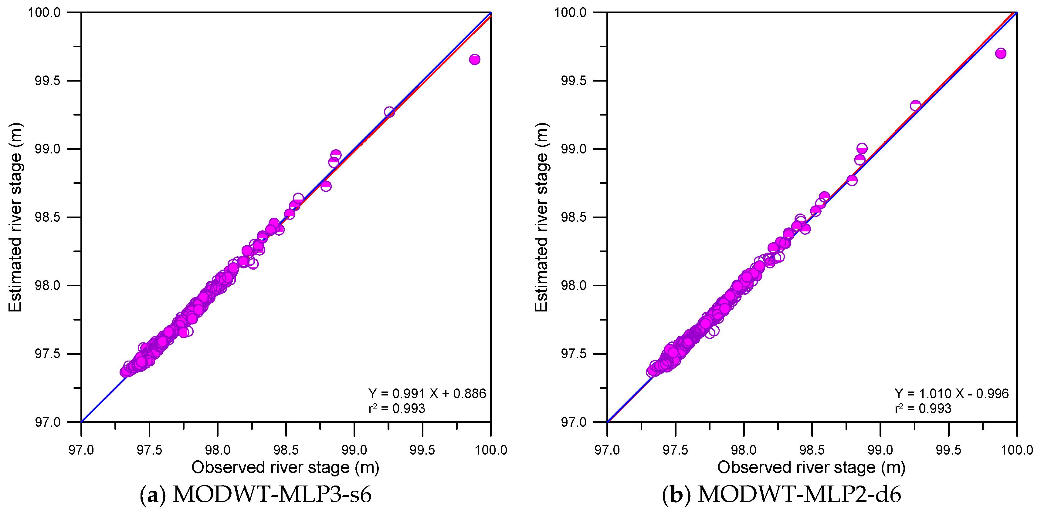
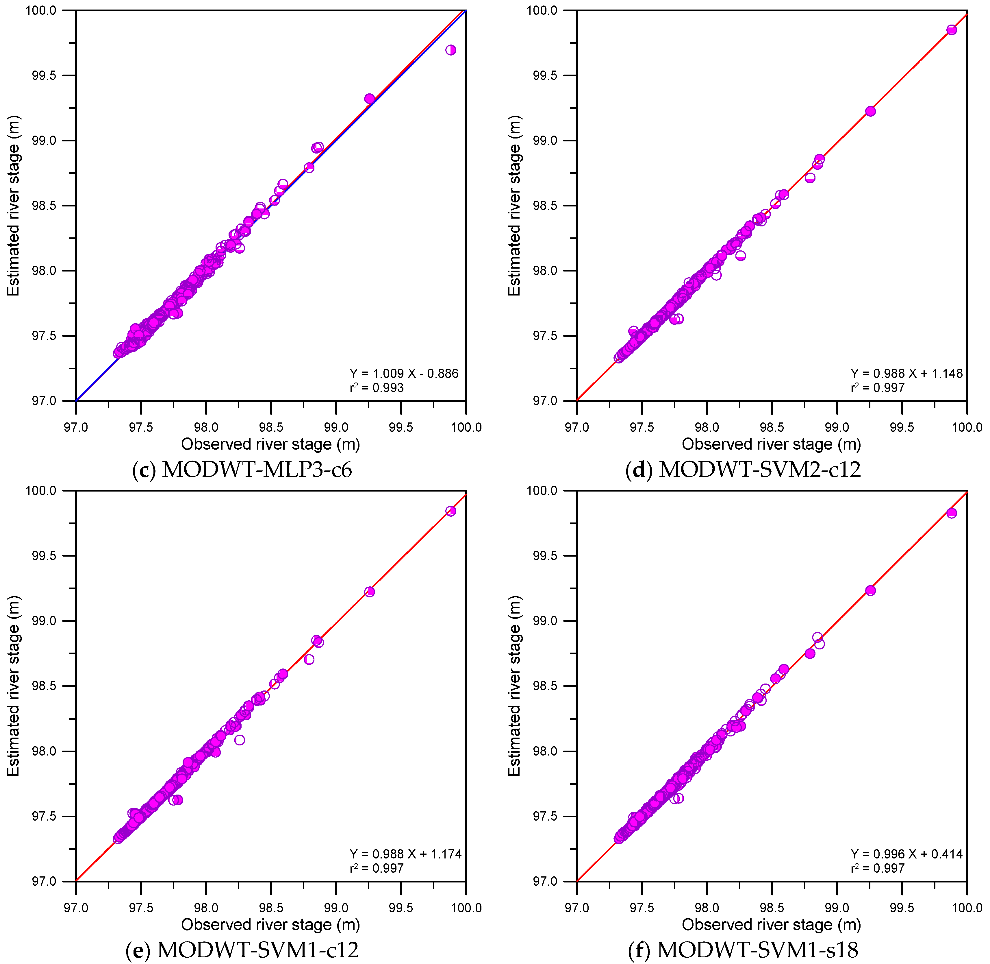
This study compared the accuracy of single, DWT- and MODWT-based models graphically. The graphical comparison included scatter plots, error time series plots and error boxplots. Figure 9, Figure 10 and Figure 11 show the scatter plots for the single, DWT- and MODWT-based models during the testing period.
From Figure 9 and Figure 11d–f, the scatter points of the MODWT–SVM models were closer to y = x lines (blue lines) than those of the single models. The best-fitting lines (red lines) of the MODWT–SVM models were closer to the y = x lines than those of the single models. These results indicated that the MODWT–SVM models were more accurate than the single models. From Figure 10 and Figure 11, the scatter points of the MODWT–SVM and DWT–MLP models were located closer to the y = x lines than those of the DWT–SVM and MODWT–MLP models. The best-fitting lines of the MODWT–SVM and DWT–MLP models were closer to the y = x lines than those of the DWT–SVM and MODWT–MLP models. These results indicated that the MODWT–SVM and DWT–MLP models were more accurate than the DWT–SVM and MODWT–MLP models.
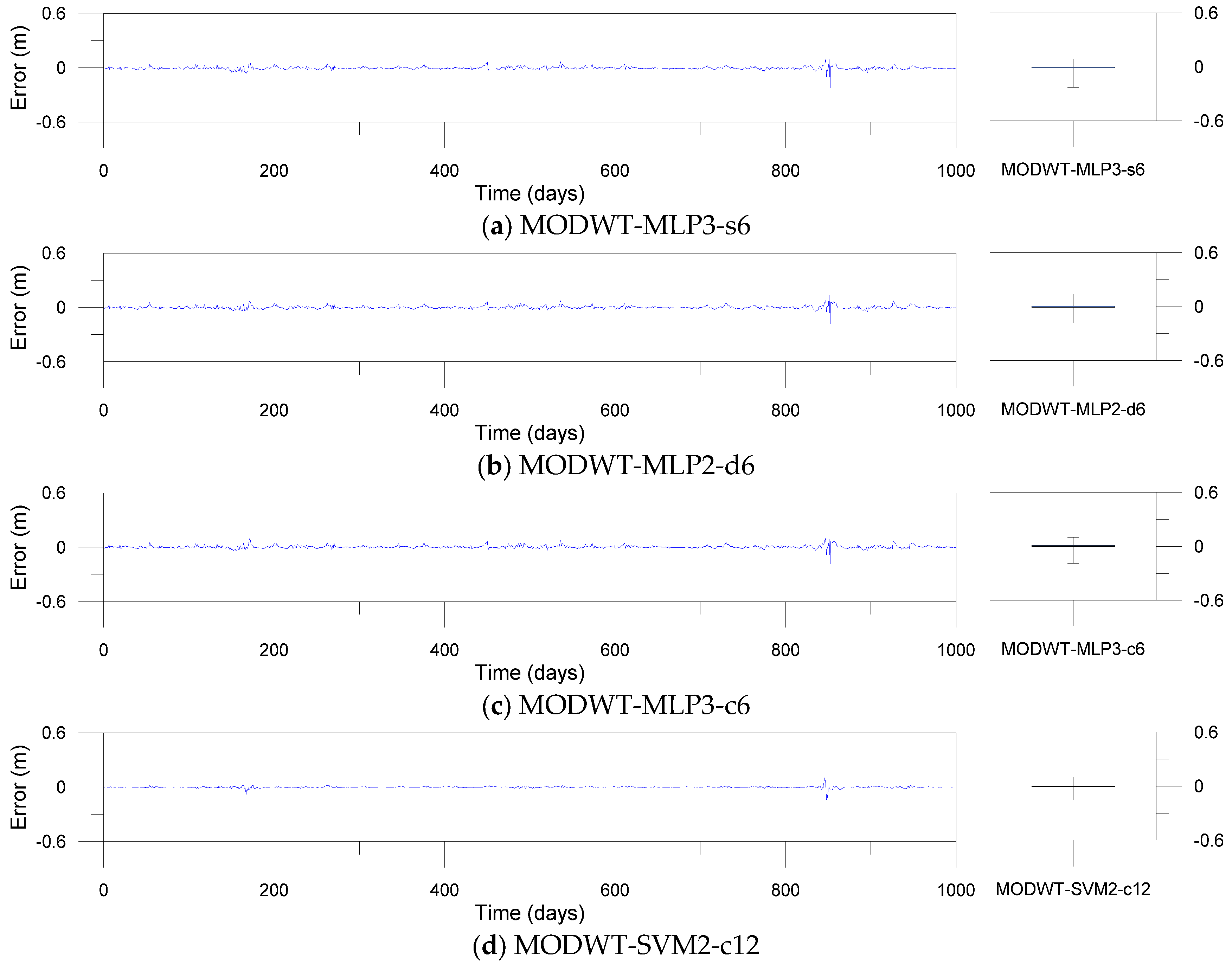
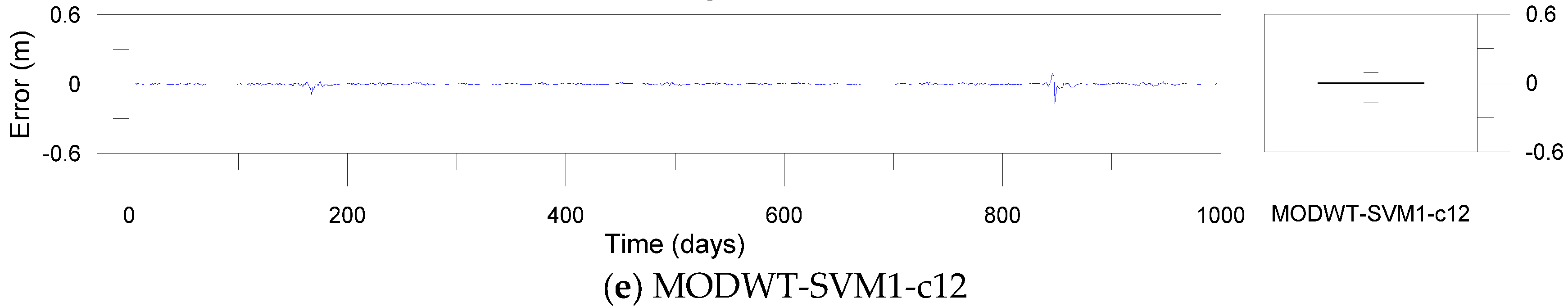
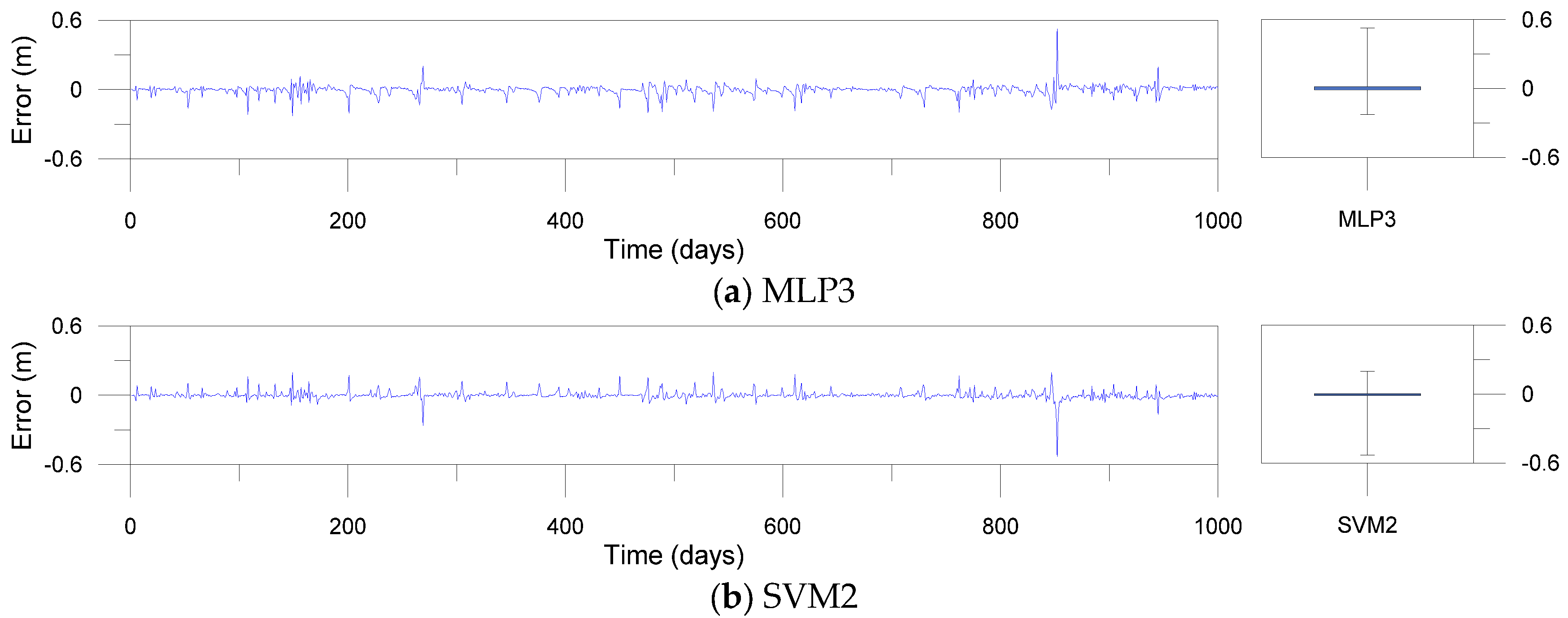
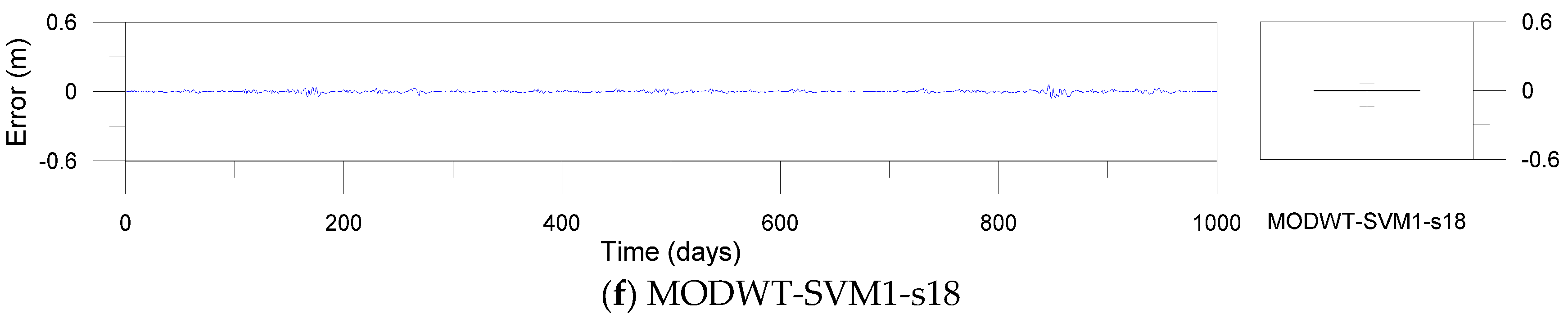
Figure 12, Figure 13 and Figure 14 show error time series plots and error boxplots for the single, DWT- and MODWT-based models during the testing period. The error is defined as the difference between the estimated and observed river stage time series as follows:
where is the ith error; is the ith estimated river stage value; and is the ith observed river stage value. The error boxplots summarize the distribution of the error values graphically. From Figure 12 and Figure 13d–f, the errors of the MODWT–SVM models were lower than those of the single models. From Figure 13 and Figure 14, the errors of the DWT–MLP and MODWT–SVM models were lower than those of the MODWT–MLP and DWT–SVM models. From Figure 12, Figure 13 and Figure 14, it can be seen that the MODWT–SVM models produced lower errors than the other models. These results indicated that the MODWT–SVM models were more accurate than the single models. The DWT–MLP and MODWT–SVM models produced more accurate results than the MODWT–MLP and DWT–SVM models. Also, the MODWT–SVM models were more accurate than the other models, based on the graphical comparison. Consequently, the MODWT–SVM and DWT–MLP–d18 models were found to produce better performance and accuracy than the other models, based on the performance assessment and graphical comparison. The MODWT–SVM1–c12 model was the optimal model among all the models. These indicated that the model performance depended on the input combination and mother wavelets, and the MODWT–SVM model using the c12 mother wavelet can improve model performance and accuracy in daily river stage modeling.
4. Conclusions
This study proposes a conjunction model of MODWT, SVM and GA for modeling daily river stages. MODWT was adopted for decomposing an original river stage time series into sub-time series (detail and approximation components). The SVM computed the daily river stages using sub-time series as inputs. The GA was adopted for selecting the optimal hyperparameters of the SVM. The performance of the MODWT–SVM models was compared with that of the single models (MLP3 and SVM2 models), DWT-based models (DWT–MLP and DWT–SVM models) and the MODWT–MLP models. The model performance for the overall stage was assessed based on the statistical indices (efficiency and effectiveness indices) and a graphical comparison. Furthermore, the model performance was assessed more specifically for the low, medium and high stages based on the statistical indices. The main conclusions are summarized as follows:
- (1)
- For the overall stage, the MODWT–SVM models achieve better efficiency and effectiveness based on the statistical indices, and are more accurate than the single models based on the graphical comparison. For the low, medium and high stages, the MODWT–SVM models perform better than the single models, in terms of efficiency and effectiveness. These results indicate that the conjunction of MODWT, SVM and GA can improve the performance of SVM models and outperform single models in daily river stage modeling.
- (2)
- For the overall stage, the MODWT–SVM models achieve better efficiency and effectiveness based on the statistical indices, and are more accurate than the MODWT–MLP and DWT-based models based on the graphical comparison. For the low and high stages, the MODWT–SVM models performed better than the MODWT–MLP and DWT-based models, in terms of efficiency and effectiveness. For the medium stage, the DWT–MLP models outperform the MODWT–SVM models, in terms of the statistical indices. These results demonstrate that the MODWT–based models using the SVM model can improve model performance and accuracy better than those using the MLP model in daily river stage modeling. Also, hybrid models coupling MODWT, SVM and GA can enhance model performance and accuracy in daily river stage modeling as compared with those combined with DWT.
- (3)
- The MODWT–SVM2–c12 model achieves the best efficiency for the overall, low and high stages, based on the efficiency indices; the MODWT–SVM1–c12 model for the low stage; the DWT–MLP1–d18 model for the medium stage; and the MODWT–SVM1–s18 model for the high stage. Also, the MODWT–SVM1–c12 model achieves the best effectiveness for the overall and low stages; the MODWT–SVM2–c12 model for the overall, low, medium and high stages; and the MODWT–SVM1–s18 model for the high stage. These results indicate that the performance of the MODWT–SVM models is dependent on input combination and mother wavelets. Furthermore, the MODWT–SVM model using the c12 mother wavelet can improve model efficiency and effectiveness in daily river stage modeling. Therefore, the results obtained from this study demonstrate that the conjunction of MODWT, SVM and GA can be an efficient and effective method for modeling daily river stages.
This study investigated the performance of single and hybrid models for a single watershed. In order to enhance the applicability of the models, a hydrological modeling approach which utilizes the river stage modeling approach that was proposed in this study for different hydrological, geographical and climate conditions can be suggested for future study.
Author Contributions
Youngmin Seo designed this research, reviewed literature, developed models, and prepared this manuscript; Yunyoung Choi reviewed model conceptualization and revised the manuscript; Jeongwoo Choi supervised the research and revised the manuscript.
Conflicts of Interest
The authors declare no conflict of interest.
Appendix A. Model Efficiency Indices
- Coefficient of efficiency (CE): ,
- Index of agreement (d): ,
- Coefficient of determination (r2): ,
- Root-mean-square error (RMSE): ,
- Mean absolute error (MAE): ,
- Mean squared relative error (MSRE): ,
- Mean higher order error (MS4E): ,
where is the ith estimated river stage value, is the ith observed river stage value, is the average of the observed river stage values, is the average of the estimated river stage values, and N is the data length.
Appendix B. Model Effectiveness Indices
- Average absolute relative error (AARE): ,
- Threshold statistics (TS): ,
where is the total number of estimated river stage data in which the absolute relative error is less than x%.
References
- Besaw, L.E.; Rizzo, D.M.; Bierman, P.R.; Hackett, W.R. Advances in ungauged streamflow prediction using artificial neural networks. J. Hydrol. 2010, 386, 27–37. [Google Scholar] [CrossRef]
- Kim, S.; Shiri, J.; Kisi, O. Pan evaporation modeling using neural computing approach for different climatic zones. Water Resour. Manag. 2012, 26, 3231–3249. [Google Scholar] [CrossRef]
- Awchi, T.A. River discharges forecasting in northern Iraq using different ANN techniques. Water Resour. Manag. 2014, 28, 801–814. [Google Scholar] [CrossRef]
- Chen, L.; Singh, V.P.; Guo, S.; Zhou, J.; Ye, L. Copula entropy coupled with artificial neural network for rainfall-runoff simulation. Stoch. Environ. Res. Risk Assess. 2014, 28, 1755–1767. [Google Scholar] [CrossRef]
- Daliakopoulos, L.N.; Tsanis, L.K. Comparison of an artificial neural network and a conceptual rainfall-runoff model in the simulation of ephemeral streamflow. Hydrol. Sci. J. 2016, 61, 2765–2774. [Google Scholar] [CrossRef]
- Ehsani, N.; Fekete, B.M.; Vörösmarty, C.J.; Tessler, Z.D. A neural network based general reservoir operation scheme. Stoch. Env. Res. Risk Assess. 2016, 30, 1151–1166. [Google Scholar] [CrossRef]
- Safari, M.-J.-S.; Aksoy, H.; Mohammadi, M. Artificial neural network and regression models for flow velocity at sediment incipient deposition. J. Hydrol. 2016, 541, 1420–1429. [Google Scholar] [CrossRef]
- Seo, Y.; Kim, S.; Kisi, O.; Singh, V.P. Daily water level forecasting using wavelet decomposition and artificial intelligence techniques. J. Hydrol. 2015, 520, 224–243. [Google Scholar] [CrossRef]
- Seo, Y.; Kim, S.; Kisi, O.; Singh, V.P.; Parasuraman, K. River stage forecasting using wavelet packet decomposition and machine learning models. Water Resour. Manag. 2016, 30, 4011–4035. [Google Scholar] [CrossRef]
- Adamowski, J.; Sun, K. Development of a coupled wavelet transform and neural network method for flow forecasting of non-perennial rivers in semi-arid watershed. J. Hydrol. 2010, 390, 85–91. [Google Scholar] [CrossRef]
- Kisi, O.; Shiri, J.; Nazemi, A.H. A wavelet-genetic programming model for predicting short-term and long-term air temperatures. J. Civ. Eng. Urban. 2011, 1, 25–37. [Google Scholar]
- Okkan, U.; Serbes, Z.A. The combined use of wavelet transform and black box models in reservoir inflow modeling. J. Hydrol. Hydromech. 2013, 61, 112–119. [Google Scholar] [CrossRef]
- Ravikumar, K.; Tamilselvan, S. On the use of wavelets packet decomposition for time series prediction. Appl. Math. Sci. 2014, 8, 2847–2858. [Google Scholar] [CrossRef]
- Raghavendera, N.S.; Deka, P.C. Forecasting monthly groundwater level fluctuations in coastal aquifers using hybrid wavelet packet-support vector regression. Cogent Eng. 2015, 2, 999414. [Google Scholar] [CrossRef]
- Cornish, C.R.; Bretherton, C.S.; Percival, D.B. Maximal overlap wavelet statistical analysis with application to atmospheric turbulence. Bound.-Layer Meteorol. 2006, 119, 339–374. [Google Scholar] [CrossRef]
- Tiwari, M.K.; Chatterjee, C. Development of an accurate and reliable hourly flood forecasting model using wavelet-bootstrap-ANN (WBANN) hybrid approach. J. Hydrol. 2010, 394, 458–470. [Google Scholar] [CrossRef]
- Nason, G. Wavelet Methods in Statistics with R; Springer: New York, NY, USA, 2008; ISBN 978-0-387-75961-6. [Google Scholar]
- Mallat, S.G. A theory for multiresolution signal decomposition: the wavelet representation. IEEE Trans. Pattern Anal. Mach. Intell. 1989, 11, 674–693. [Google Scholar] [CrossRef]
- Percival, D.B.; Walden, A.T. Wavelet Methods for Time Series Analysis; Cambridge University Press: Cambridge, UK, 2000; ISBN 978-0-521-68508-5. [Google Scholar]
- Nourani, V.; Alami, M.T.; Aminfar, M.H. A combined neural-wavelet model for prediction of Ligvanchai watershed precipitation. Eng. Appl. Artif. Intell. 2009, 22, 466–472. [Google Scholar] [CrossRef]
- Günther, F.; Fritsch, S. Neuralnet: Training of neural networks. R J. 2010, 2, 30–38. [Google Scholar]
- Vapnik, V.N. Statistical Learning Theory; Wiley: New York, NY, USA, 1998; ISBN 978-0-471-03003-4. [Google Scholar]
- Noori, R.; Karbassi, A.R.; Moghaddamnia, A.; Han, D.; Zokaei-Ashtiani, M.H.; Farokhnia, A.; Ghafari Gousheh, M. Assessment of input variables determination on the SVM model performance using PCA, gamma test and forward selection techniques for monthly stream flow prediction. J. Hydrol. 2011, 401, 177–189. [Google Scholar] [CrossRef]
- Sivanandam, S.N.; Deepa, S.N. Introduction to Genetic Algorithms; Springer: Berlin, Germany, 2007; ISBN 978-3-540-73189-4. [Google Scholar]
- Scrucca, L. GA: A package for genetic algorithms in R. J. Stat. Softw. 2013, 53, 1–37. [Google Scholar] [CrossRef]
- Obitko, M. Introduction to Genetic Algorithms. 1998. Available online: http://www.obitko.com/tutorials/genetic-algorithms/ (accessed on 28 June 2017).
- Dawson, C.W.; Wilby, R.L. Hydrological modelling using artificial neural networks. Prog. Phys. Geogr. 2001, 25, 80–108. [Google Scholar] [CrossRef]
- Dawson, C.W.; Abrahart, R.J.; See, L.M. HydroTest: A web-based toolbox of evaluation metrics for the standardised assessment of hydrological forecasts. Environ. Model. Softw. 2007, 22, 1034–1052. [Google Scholar] [CrossRef]
- Jain, A.; Srinivasulu, S. Development of effective and efficient rainfall-runoff models using integration of deterministic, real-coded genetic algorithms and artificial neural network techniques. Water Resour. Res. 2004, 40, W04302. [Google Scholar] [CrossRef]
- Srinivasulu, S.; Jain, A. A comparative analysis of training methods for artificial neural network rainfall-runoff models. Appl. Soft Comput. 2006, 6, 295–306. [Google Scholar] [CrossRef]
- Jain, A.; Kumar, A.M. Hybrid neural network models for hydrologic time series forecasting. Appl. Soft Comput. 2007, 7, 585–592. [Google Scholar] [CrossRef]
- Panagoulia, D.; Tsekouras, G.J.; Kousiouris, G. A multi-stage methodology for selecting input variables in ANN forecasting of river flows. Glob. NEST J. 2017, 19, 49–57. [Google Scholar]
- Wu, C. Hydrological Predictions Using Data-Driven Models Coupled with Data Preprocessing Techniques. Ph.D. Thesis, The Hong Kong Polytechnic University, Kowloon, Hong Kong, 2010. [Google Scholar]
- Venables, W.N.; Ripley, B.D. Modern Applied Statistics with S, 4th ed.; Springer: New York, NY, USA, 2002; ISBN 978-0-387-21706-2. [Google Scholar]
Figure 1.
Study area and streamflow gauging stations.
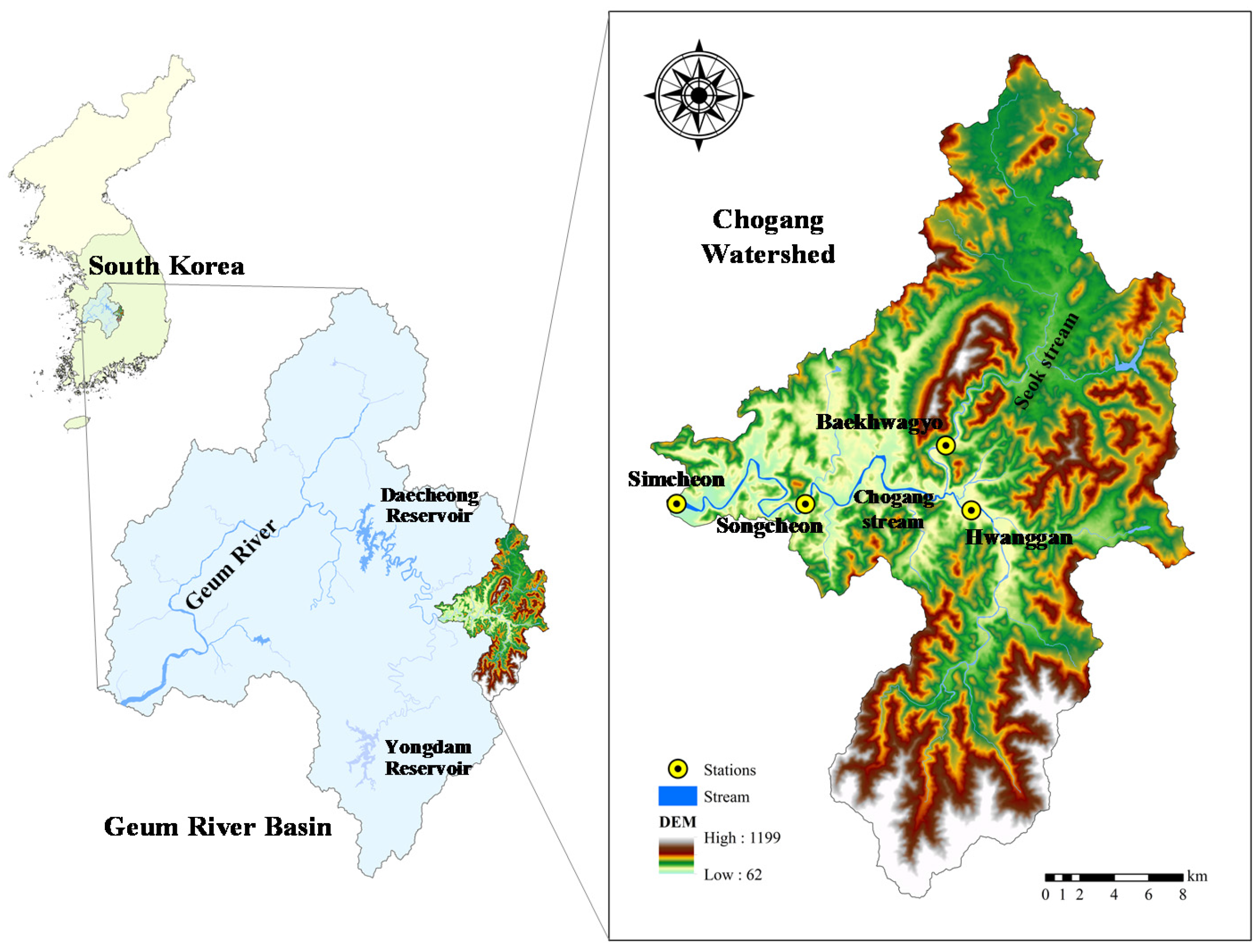
Figure 2.
Flowchart for three-level DWT.
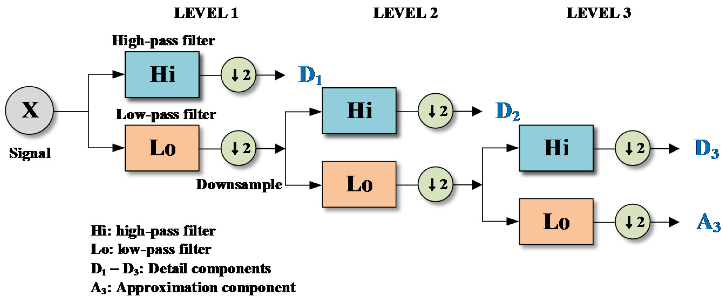
Figure 3.
Flowchart for three-level MODWT.
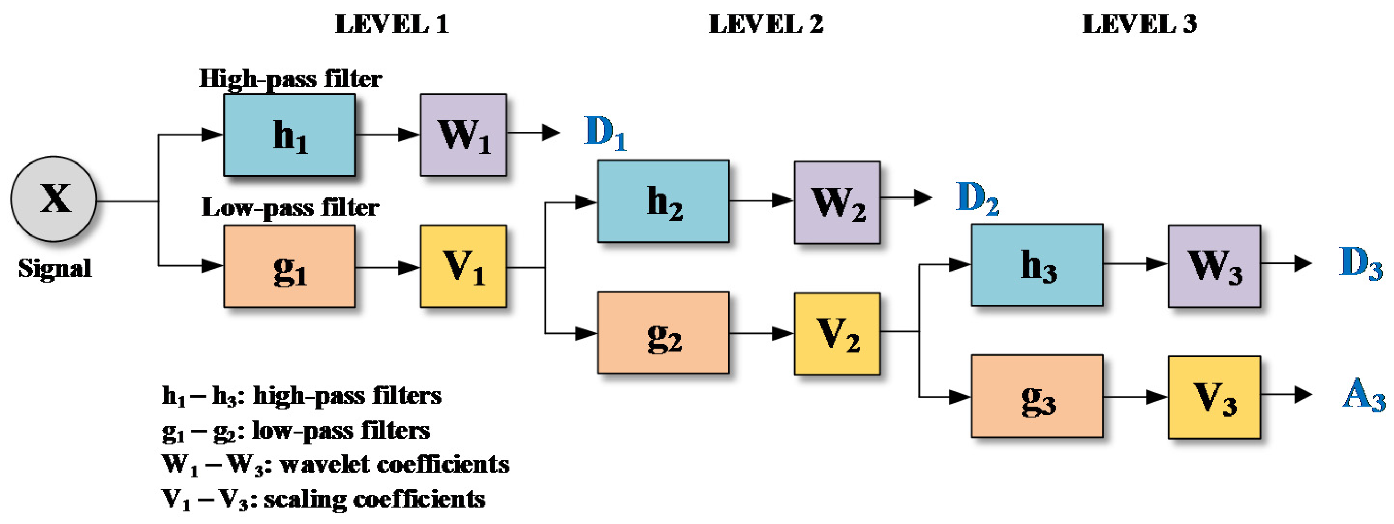
Figure 4.
An example of MLP model architecture.
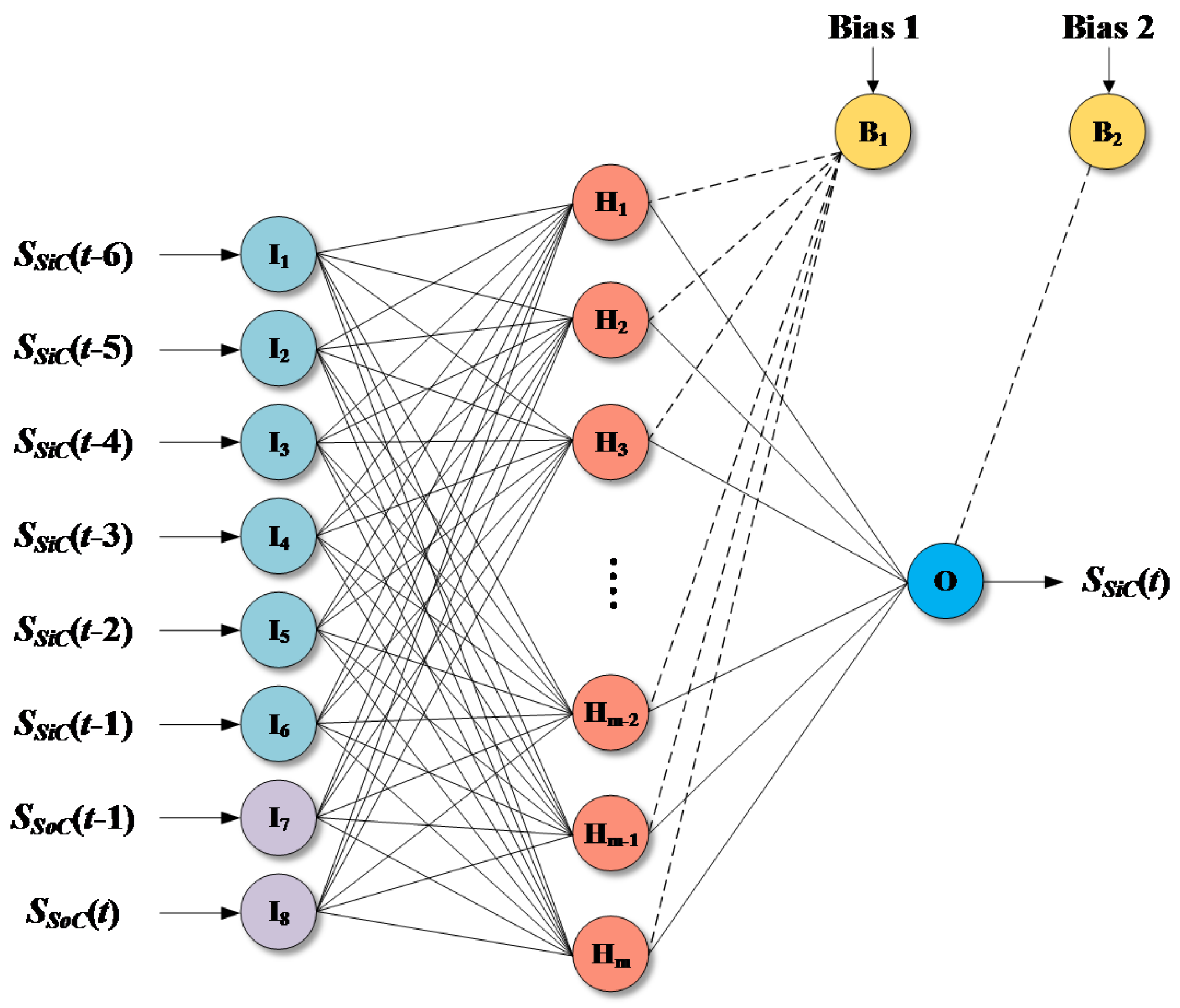
Figure 5.
An example of SVM model architecture.
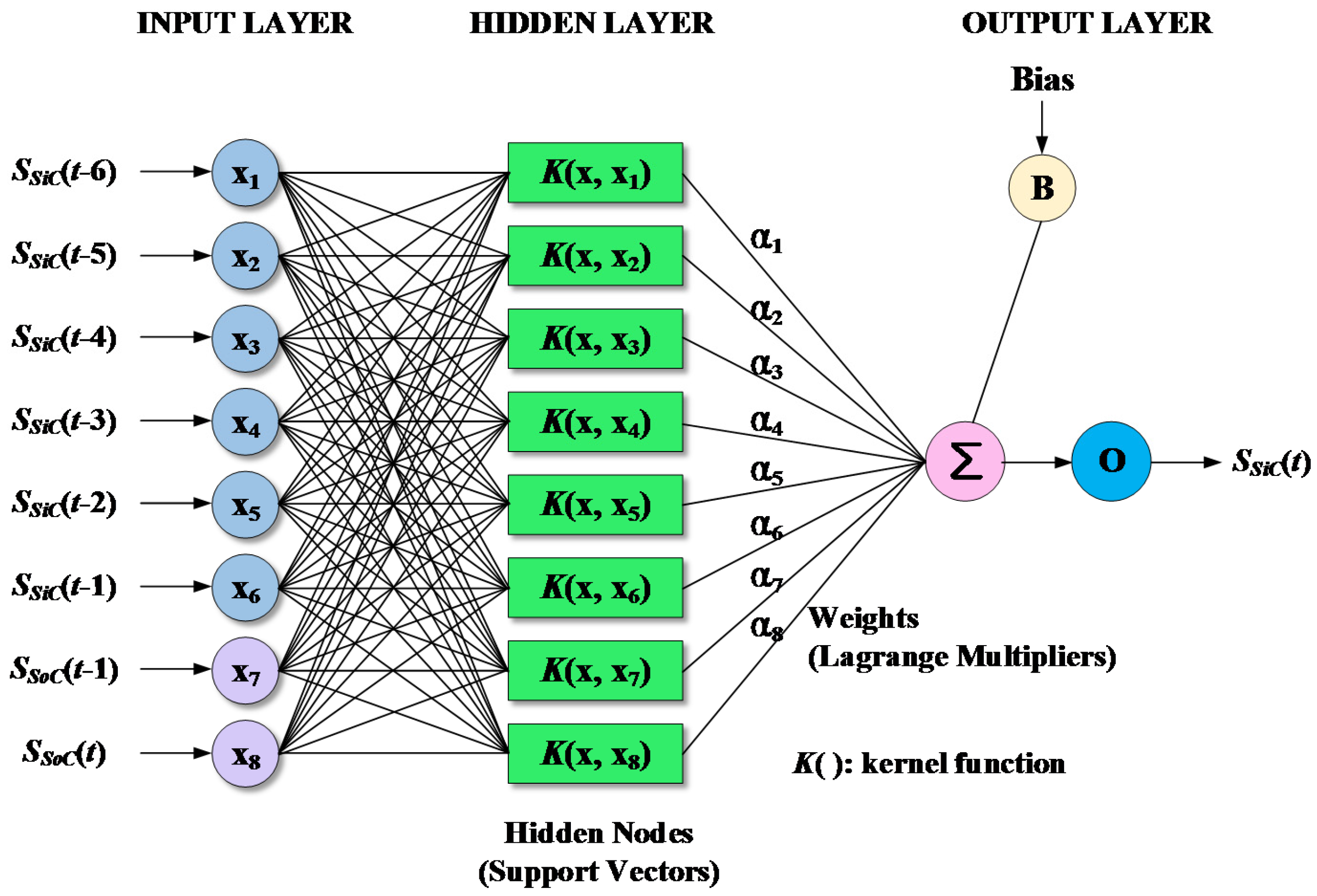
Figure 6.
Flowchart of river stage modeling using DWT and MODWT.

Figure 7.
Sub-time series (a–d) decomposed by DWT and original river stage time series (e) at the Songcheon gauging station.
Figure 7.
Sub-time series (a–d) decomposed by DWT and original river stage time series (e) at the Songcheon gauging station.

Figure 8.
Sub-time series (a–d) decomposed by MODWT and original river stage time series (e) at the Songcheon gauging station.
Figure 8.
Sub-time series (a–d) decomposed by MODWT and original river stage time series (e) at the Songcheon gauging station.
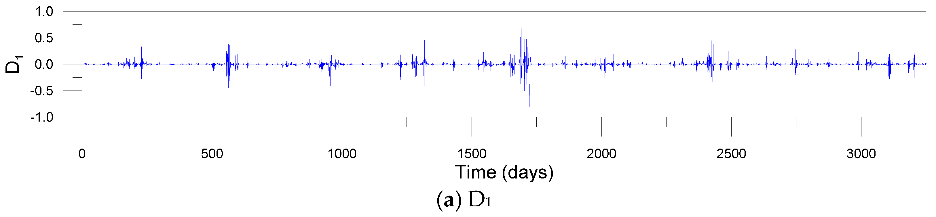

Figure 9.
Scatter plots for the MLP and SVM models.
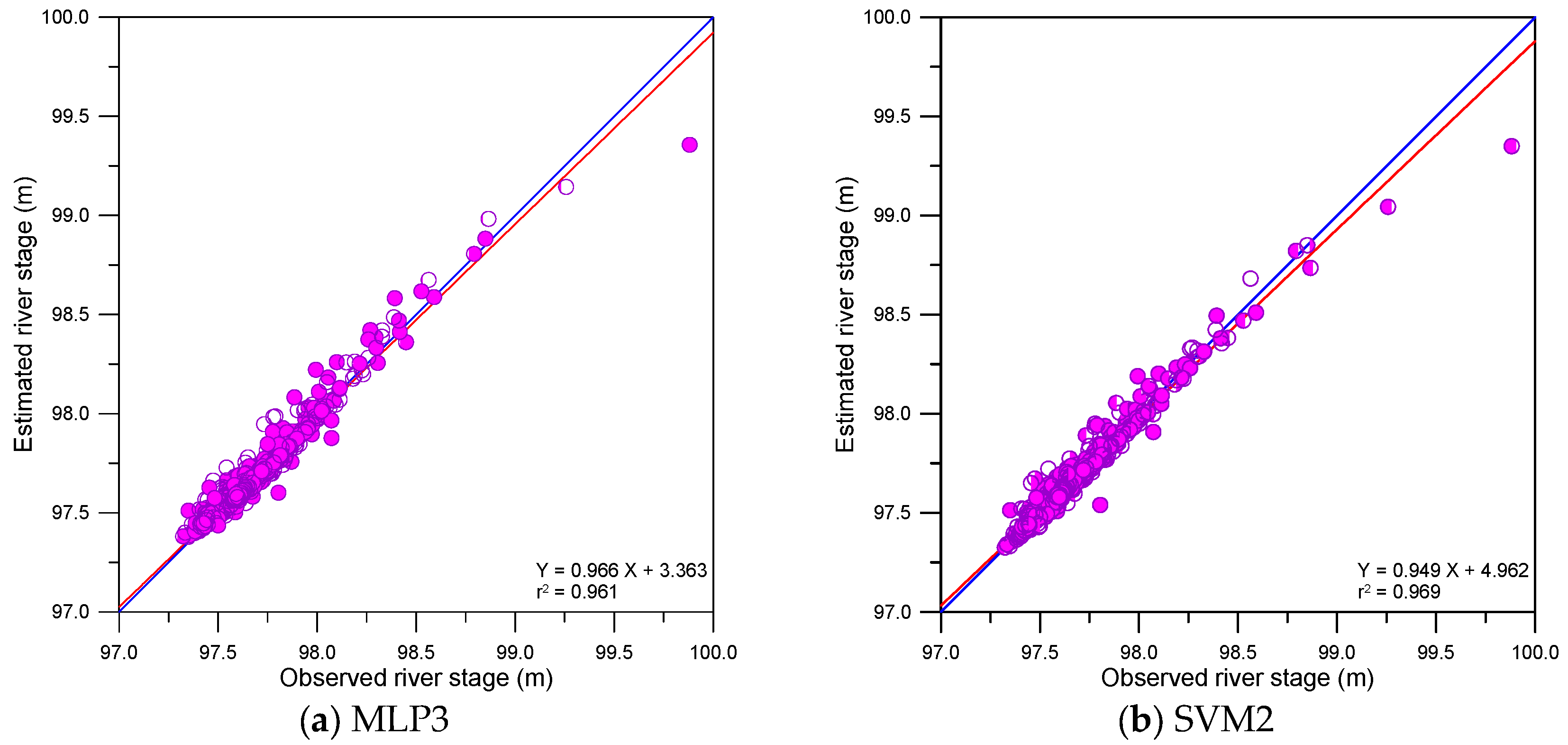
Figure 10.
Scatter plots for DWT-based models.
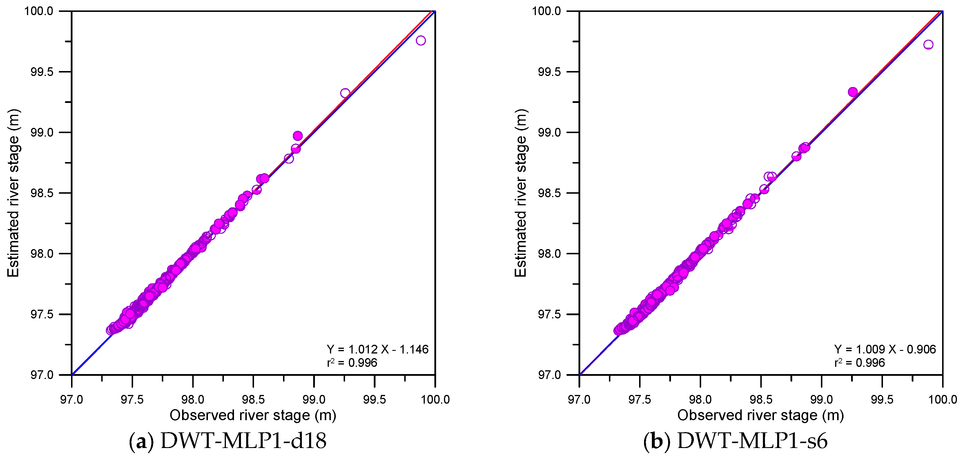

Figure 11.
Scatter plots for the MODWT-based models.


Figure 12.
Error time series plots and error boxplots for the MLP and SVM models.

Figure 13.
Error time series plots and error boxplots for the DWT-based models.
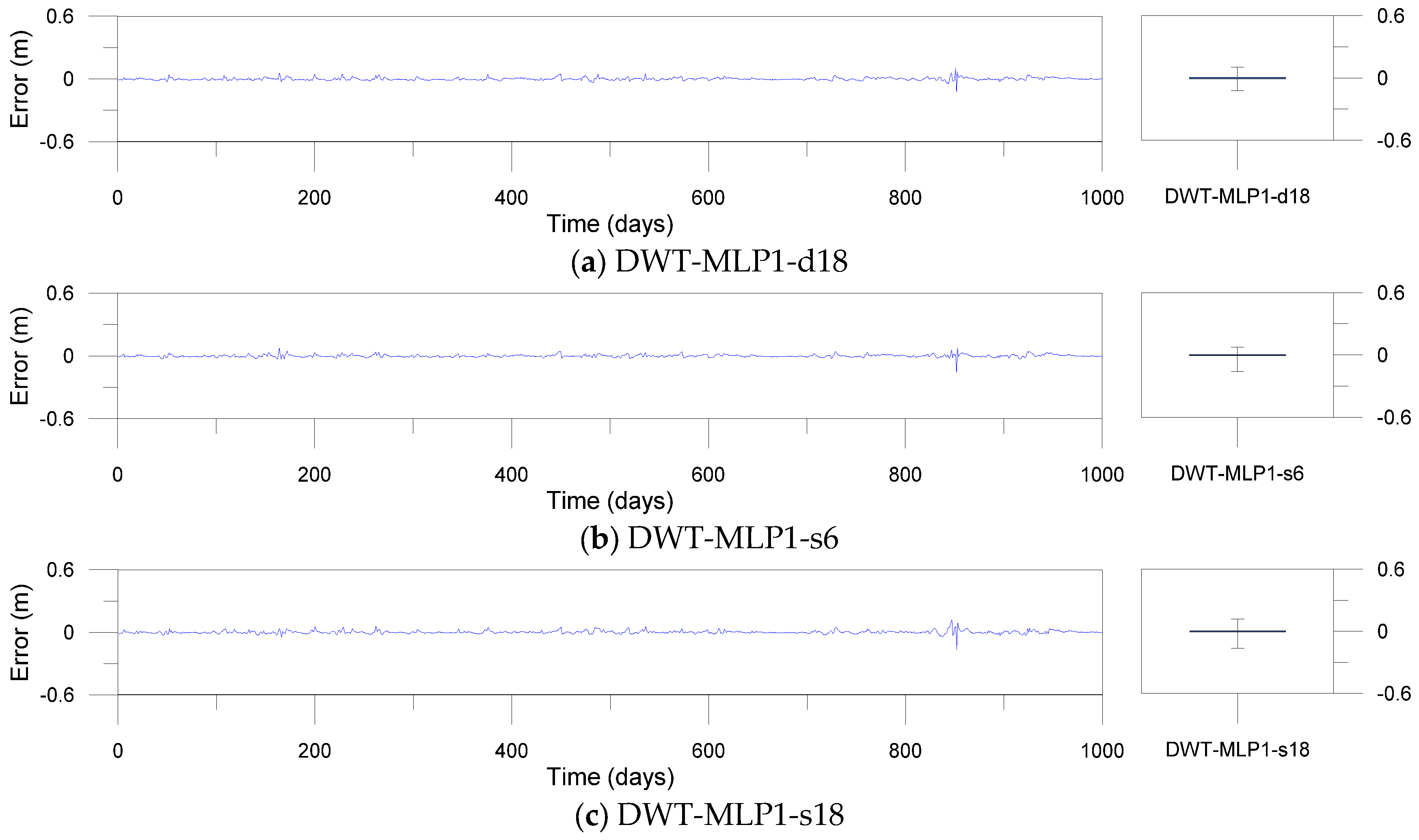
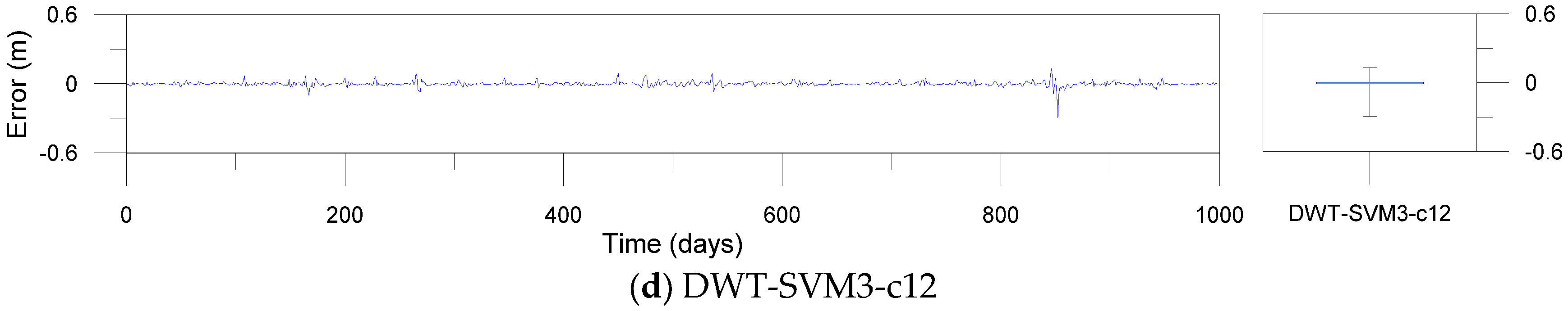
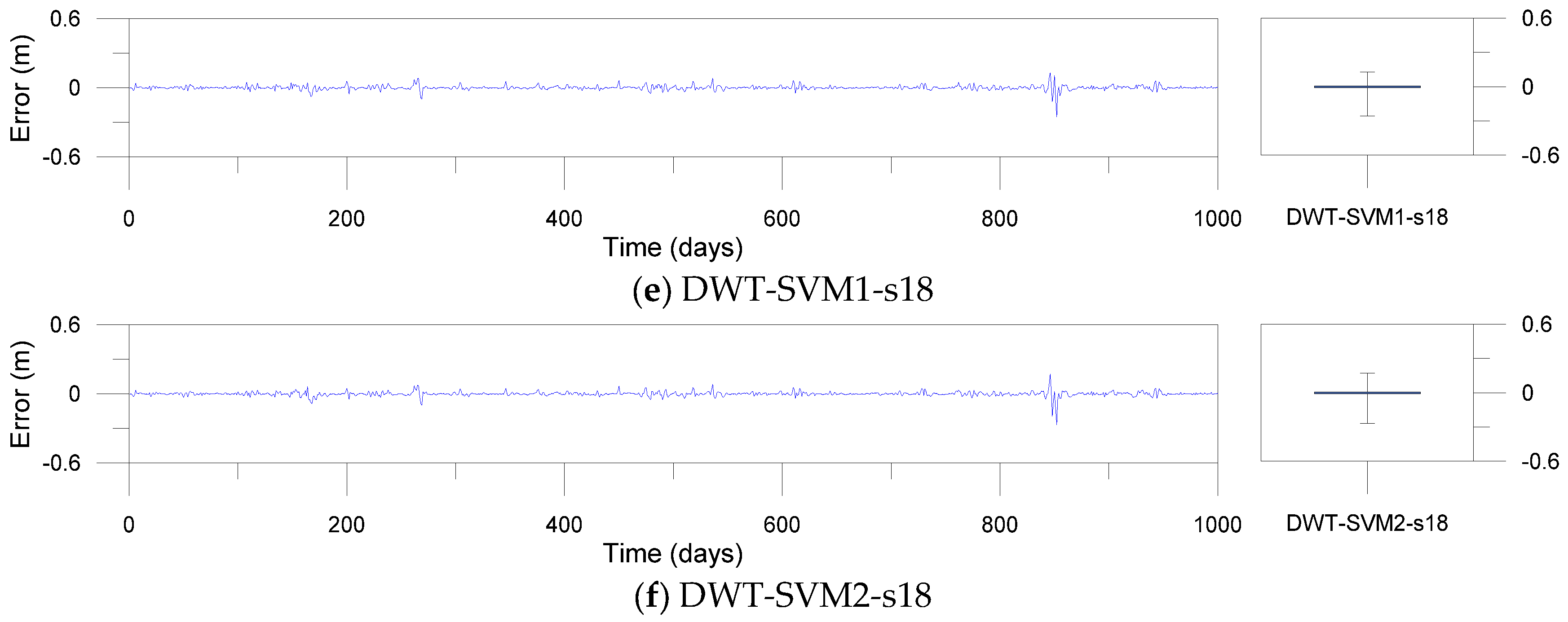
Figure 14.
Error time series plots and error boxplots for the MODWT-based models.


Table 1.
Input combination for model development.
| Input Sets | Input Variables | Output Variables |
|---|---|---|
| Set 1 | SSiC(t-6), SSiC(t-5), SSiC(t-4), SSiC(t-3), SSiC(t-2), SSiC(t-1), SSoC(t-1), SSoC(t) | SSiC(t) |
| Set 2 | SSiC(t-6), SSiC(t-5), SSiC(t-4), SSiC(t-3), SSiC(t-2), SSiC(t-1), SSoC(t-1), SSoC(t), SBH(t-1), SBH(t) | SSiC(t) |
| Set 3 | SSiC(t-6), SSiC(t-5), SSiC(t-4), SSiC(t-3), SSiC(t-2), SSiC(t-1), SSoC(t-1), SSoC(t), SBH(t-1), SBH(t), SHG(t-1), SHG(t) | SSiC(t) |
S: daily river stage, SiC: Simcheon, SoC: Songcheon, BH: Baekhwagyo, HG: Hwanggan.
Table 2.
Comparison of higher performance models for the overall stage.
| Models | CE | d | r2 | RMSE (m) | MAE (m) | MSRE (10−5) | MS4E (10−6 m4) | AARE (%) | TS0.01 (%) | TS0.02 (%) | TS0.05 (%) | TS0.10 (%) | TS0.50 (%) | TS1.00 (%) |
|---|---|---|---|---|---|---|---|---|---|---|---|---|---|---|
| MLP3 | 0.961 | 0.990 | 0.961 | 0.0419 | 0.0243 | 492.090 | 99.187 | 0.025 | 35.7 | 62.8 | 88.3 | 96.2 | 99.9 | 100.0 |
| SVM2 | 0.969 | 0.992 | 0.969 | 0.0374 | 0.0196 | 357.683 | 98.212 | 0.026 | 35.0 | 61.7 | 87.5 | 95.8 | 99.9 | 100.0 |
| DWT-MLP1-d18 | 0.996 | 0.999 | 0.996 | 0.0129 | 0.0089 | 60.130 | 0.482 | 0.009 | 68.0 | 92.1 | 99.4 | 99.8 | 100.0 | 100.0 |
| DWT-MLP1-s6 | 0.996 | 0.999 | 0.996 | 0.0130 | 0.0089 | 54.750 | 0.765 | 0.009 | 68.4 | 91.7 | 99.4 | 99.9 | 100.0 | 100.0 |
| DWT-MLP1-s18 | 0.995 | 0.999 | 0.995 | 0.0153 | 0.0097 | 91.610 | 1.208 | 0.010 | 68.3 | 88.3 | 99.1 | 99.8 | 100.0 | 100.0 |
| DWT-SVM3-c12 | 0.990 | 0.997 | 0.991 | 0.0211 | 0.0117 | 125.750 | 9.914 | 0.012 | 63.2 | 85.3 | 96.9 | 99.5 | 100.0 | 100.0 |
| DWT-SVM1-s18 | 0.989 | 0.997 | 0.990 | 0.0218 | 0.0117 | 119.140 | 9.382 | 0.012 | 64.2 | 84.0 | 97.2 | 99.3 | 100.0 | 100.0 |
| DWT-SVM2-s18 | 0.989 | 0.997 | 0.990 | 0.0221 | 0.0114 | 124.370 | 11.197 | 0.012 | 65.4 | 84.5 | 97.3 | 99.3 | 100.0 | 100.0 |
| MODWT-MLP3-s6 | 0.993 | 0.998 | 0.993 | 0.0177 | 0.0119 | 91.980 | 3.250 | 0.012 | 53.8 | 85.5 | 98.7 | 99.7 | 100.0 | 100.0 |
| MODWT-MLP2-d6 | 0.993 | 0.998 | 0.993 | 0.0178 | 0.0114 | 94.810 | 2.051 | 0.012 | 60.4 | 84.7 | 98.0 | 99.6 | 100.0 | 100.0 |
| MODWT-MLP3-c6 | 0.993 | 0.998 | 0.993 | 0.0178 | 0.0109 | 93.410 | 2.035 | 0.011 | 64.6 | 85.6 | 97.8 | 99.7 | 100.0 | 100.0 |
| MODWT-SVM2-c12 | 0.997 | 0.999 | 0.997 | 0.0113 | 0.0049 | 29.540 | 1.430 | 0.005 | 90.1 | 97.6 | 99.3 | 99.5 | 100.0 | 100.0 |
| MODWT-SVM1-c12 | 0.997 | 0.999 | 0.997 | 0.0118 | 0.0048 | 31.020 | 1.879 | 0.005 | 91.6 | 97.2 | 99.1 | 99.7 | 100.0 | 100.0 |
| MODWT-SVM1-s18 | 0.997 | 0.999 | 0.997 | 0.0115 | 0.0068 | 32.530 | 0.657 | 0.007 | 78.7 | 94.3 | 99.5 | 99.8 | 100.0 | 100.0 |
For example, MODWT-SVM2-c12 means MODWT-based SVM model for Set 2 and c12 mother wavelet. TSx means the threshold statistics for the absolute relative error level of x%.
Table 3.
Comparison of higher performance models for the low stage.
| Models | CE | d | r2 | RMSE (m) | MAE (m) | MSRE (10−5) | MS4E (10−6 m4) | AARE (%) | TS0.01 (%) | TS0.02 (%) | TS0.05 (%) | TS0.10 (%) | TS0.50 (%) | TS1.00 (%) |
|---|---|---|---|---|---|---|---|---|---|---|---|---|---|---|
| MLP3 | 0.797 | 0.943 | 0.808 | 0.0313 | 0.0195 | 0.0103 | 10.772 | 0.0200 | 43.1 | 68.6 | 91.3 | 98.0 | 100.0 | 100.0 |
| SVM2 | 0.770 | 0.936 | 0.785 | 0.0332 | 0.0209 | 0.0116 | 13.287 | 0.0214 | 41.8 | 66.8 | 89.9 | 97.3 | 100.0 | 100.0 |
| DWT-MLP1-d18 | 0.970 | 0.992 | 0.972 | 0.0120 | 0.0087 | 0.0015 | 0.133 | 0.0090 | 68.3 | 92.0 | 99.7 | 100.0 | 100.0 | 100.0 |
| DWT-MLP1-s6 | 0.973 | 0.993 | 0.976 | 0.0114 | 0.0088 | 0.0014 | 0.086 | 0.0090 | 67.2 | 92.5 | 99.8 | 100.0 | 100.0 | 100.0 |
| DWT-MLP1-s18 | 0.954 | 0.988 | 0.954 | 0.0148 | 0.0097 | 0.0023 | 0.625 | 0.0100 | 67.2 | 87.7 | 99.1 | 99.8 | 100.0 | 100.0 |
| DWT-SVM3-c12 | 0.952 | 0.987 | 0.952 | 0.0152 | 0.0094 | 0.0024 | 0.930 | 0.0096 | 69.4 | 88.6 | 98.3 | 99.8 | 100.0 | 100.0 |
| DWT-SVM1-s18 | 0.958 | 0.989 | 0.958 | 0.0143 | 0.0085 | 0.0021 | 0.768 | 0.0088 | 73.6 | 89.7 | 98.3 | 99.8 | 100.0 | 100.0 |
| DWT-SVM2-s18 | 0.954 | 0.988 | 0.954 | 0.0149 | 0.0085 | 0.0023 | 1.665 | 0.0087 | 74.7 | 89.9 | 98.6 | 99.8 | 100.0 | 100.0 |
| MODWT-MLP3-s6 | 0.958 | 0.989 | 0.965 | 0.0142 | 0.0109 | 0.0021 | 0.259 | 0.0112 | 53.4 | 88.0 | 99.4 | 100.0 | 100.0 | 100.0 |
| MODWT-MLP2-d6 | 0.959 | 0.989 | 0.960 | 0.0141 | 0.0102 | 0.0021 | 0.271 | 0.0104 | 61.3 | 87.7 | 99.2 | 100.0 | 100.0 | 100.0 |
| MODWT-MLP3-c6 | 0.962 | 0.990 | 0.963 | 0.0135 | 0.0089 | 0.0019 | 0.399 | 0.0091 | 69.7 | 90.0 | 99.2 | 99.8 | 100.0 | 100.0 |
| MODWT-SVM2-c12 | 0.992 | 0.998 | 0.992 | 0.0063 | 0.0033 | 0.0004 | 0.174 | 0.0034 | 95.8 | 99.4 | 99.7 | 99.8 | 100.0 | 100.0 |
| MODWT-SVM1-c12 | 0.992 | 0.998 | 0.992 | 0.0064 | 0.0030 | 0.0004 | 0.164 | 0.0031 | 97.5 | 99.5 | 99.5 | 100.0 | 100.0 | 100.0 |
| MODWT-SVM1-s18 | 0.990 | 0.998 | 0.990 | 0.0069 | 0.0047 | 0.0005 | 0.030 | 0.0048 | 88.5 | 98.8 | 99.8 | 100.0 | 100.0 | 100.0 |
Table 4.
Comparison of higher performance models for the medium stage.
| Models | CE | d | r2 | RMSE (m) | MAE (m) | MSRE (10−5) | MS4E (10−6 m4) | AARE (%) | TS0.01 (%) | TS0.02 (%) | TS0.05 (%) | TS0.10 (%) | TS0.50 (%) | TS1.00 (%) |
|---|---|---|---|---|---|---|---|---|---|---|---|---|---|---|
| MLP3 | 0.603 | 0.911 | 0.723 | 0.0385 | 0.0248 | 0.0155 | 29.965 | 0.0253 | 24.7 | 58.7 | 89.4 | 97.5 | 100.0 | 100.0 |
| SVM2 | 0.606 | 0.913 | 0.730 | 0.0383 | 0.0246 | 0.0154 | 27.321 | 0.0252 | 25.8 | 58.3 | 89.8 | 97.2 | 100.0 | 100.0 |
| DWT-MLP1-d18 | 0.977 | 0.995 | 0.984 | 0.0093 | 0.0069 | 0.0009 | 0.051 | 0.0070 | 77.4 | 96.8 | 100.0 | 100.0 | 100.0 | 100.0 |
| DWT-MLP1-s6 | 0.975 | 0.994 | 0.980 | 0.0096 | 0.0066 | 0.0010 | 0.100 | 0.0067 | 80.2 | 95.8 | 99.3 | 100.0 | 100.0 | 100.0 |
| DWT-MLP1-s18 | 0.976 | 0.994 | 0.979 | 0.0095 | 0.0066 | 0.0009 | 0.061 | 0.0068 | 80.9 | 95.4 | 100.0 | 100.0 | 100.0 | 100.0 |
| DWT-SVM3-c12 | 0.875 | 0.970 | 0.898 | 0.0216 | 0.0124 | 0.0049 | 5.589 | 0.0127 | 58.7 | 87.6 | 96.1 | 99.3 | 100.0 | 100.0 |
| DWT-SVM1-s18 | 0.832 | 0.959 | 0.856 | 0.0251 | 0.0129 | 0.0066 | 15.514 | 0.0131 | 56.9 | 84.8 | 97.5 | 98.9 | 100.0 | 100.0 |
| DWT-SVM2-s18 | 0.854 | 0.965 | 0.874 | 0.0234 | 0.0121 | 0.0057 | 11.551 | 0.0124 | 58.7 | 85.5 | 97.5 | 98.9 | 100.0 | 100.0 |
| MODWT-MLP3-s6 | 0.936 | 0.984 | 0.949 | 0.0154 | 0.0100 | 0.0025 | 1.056 | 0.0103 | 63.3 | 90.1 | 98.9 | 99.6 | 100.0 | 100.0 |
| MODWT-MLP2-d6 | 0.946 | 0.987 | 0.951 | 0.0142 | 0.0085 | 0.0021 | 0.989 | 0.0087 | 72.1 | 91.2 | 98.9 | 99.3 | 100.0 | 100.0 |
| MODWT-MLP3-c6 | 0.945 | 0.987 | 0.952 | 0.0143 | 0.0094 | 0.0021 | 0.723 | 0.0096 | 66.1 | 88.7 | 99.3 | 99.6 | 100.0 | 100.0 |
| MODWT-SVM2-c12 | 0.952 | 0.988 | 0.955 | 0.0134 | 0.0057 | 0.0019 | 2.688 | 0.0058 | 88.3 | 97.2 | 99.3 | 99.3 | 100.0 | 100.0 |
| MODWT-SVM1-c12 | 0.950 | 0.988 | 0.953 | 0.0137 | 0.0058 | 0.0020 | 2.914 | 0.0059 | 88.3 | 96.8 | 99.3 | 99.3 | 100.0 | 100.0 |
| MODWT-SVM1-s18 | 0.940 | 0.985 | 0.946 | 0.0149 | 0.0083 | 0.0023 | 2.110 | 0.0084 | 71.7 | 93.6 | 99.3 | 99.3 | 100.0 | 100.0 |
Table 5.
Comparison of higher performance models for the high stage.
| Models | CE | d | r2 | RMSE (m) | MAE (m) | MSRE (10−5) | MS4E (10−6 m4) | AARE (%) | TS0.01 (%) | TS0.02 (%) | TS0.05 (%) | TS0.10 (%) | TS0.50 (%) | TS1.00 (%) |
|---|---|---|---|---|---|---|---|---|---|---|---|---|---|---|
| MLP3 | 0.921 | 0.979 | 0.921 | 0.0850 | 0.0518 | 0.0741 | 818.660 | 0.0527 | 20.8 | 38.7 | 67.0 | 82.1 | 99.1 | 100.0 |
| SVM2 | 0.927 | 0.981 | 0.928 | 0.0814 | 0.0502 | 0.0679 | 670.961 | 0.0511 | 17.9 | 39.6 | 67.0 | 83.0 | 99.1 | 100.0 |
| DWT-MLP1-d18 | 0.994 | 0.999 | 0.996 | 0.0229 | 0.0152 | 0.0054 | 3.743 | 0.0155 | 40.6 | 80.2 | 96.2 | 98.1 | 100.0 | 100.0 |
| DWT-MLP1-s6 | 0.993 | 0.998 | 0.995 | 0.0245 | 0.0159 | 0.0061 | 6.646 | 0.0162 | 44.3 | 76.4 | 97.2 | 99.1 | 100.0 | 100.0 |
| DWT-MLP1-s18 | 0.992 | 0.998 | 0.993 | 0.0266 | 0.0175 | 0.0072 | 7.794 | 0.0177 | 41.5 | 72.6 | 97.2 | 99.1 | 100.0 | 100.0 |
| DWT-SVM3-c12 | 0.981 | 0.995 | 0.987 | 0.0410 | 0.0237 | 0.0171 | 75.787 | 0.0241 | 37.7 | 59.4 | 90.6 | 98.1 | 100.0 | 100.0 |
| DWT-SVM1-s18 | 0.981 | 0.995 | 0.984 | 0.0412 | 0.0272 | 0.0173 | 45.099 | 0.0277 | 26.4 | 47.2 | 89.6 | 97.2 | 100.0 | 100.0 |
| DWT-SVM2-s18 | 0.978 | 0.994 | 0.984 | 0.0443 | 0.0270 | 0.0201 | 67.891 | 0.0275 | 27.4 | 49.1 | 88.7 | 97.2 | 100.0 | 100.0 |
| MODWT-MLP3-s6 | 0.987 | 0.997 | 0.987 | 0.0348 | 0.0224 | 0.0124 | 27.195 | 0.0227 | 31.1 | 58.5 | 94.3 | 98.1 | 100.0 | 100.0 |
| MODWT-MLP2-d6 | 0.985 | 0.996 | 0.987 | 0.0365 | 0.0263 | 0.0137 | 15.645 | 0.0268 | 23.6 | 49.1 | 87.7 | 98.1 | 100.0 | 100.0 |
| MODWT-MLP3-c6 | 0.984 | 0.996 | 0.986 | 0.0378 | 0.0269 | 0.0147 | 15.432 | 0.0274 | 29.2 | 50.9 | 84.9 | 99.1 | 100.0 | 100.0 |
| MODWT-SVM2-c12 | 0.994 | 0.999 | 0.995 | 0.0230 | 0.0124 | 0.0055 | 5.664 | 0.0126 | 60.4 | 87.7 | 97.2 | 98.1 | 100.0 | 100.0 |
| MODWT-SVM1-c12 | 0.993 | 0.998 | 0.994 | 0.0248 | 0.0131 | 0.0064 | 9.493 | 0.0133 | 64.2 | 84.0 | 96.2 | 99.1 | 100.0 | 100.0 |
| MODWT-SVM1-s18 | 0.996 | 0.999 | 0.996 | 0.0201 | 0.0155 | 0.0042 | 0.570 | 0.0158 | 38.7 | 68.9 | 98.1 | 100.0 | 100.0 | 100.0 |
© 2017 by the authors. Licensee MDPI, Basel, Switzerland. This article is an open access article distributed under the terms and conditions of the Creative Commons Attribution (CC BY) license (http://creativecommons.org/licenses/by/4.0/).
Share and Cite
MDPI and ACS Style
Seo, Y.; Choi, Y.; Choi, J. River Stage Modeling by Combining Maximal Overlap Discrete Wavelet Transform, Support Vector Machines and Genetic Algorithm. Water 2017, 9, 525. https://doi.org/10.3390/w9070525
AMA Style
Seo Y, Choi Y, Choi J. River Stage Modeling by Combining Maximal Overlap Discrete Wavelet Transform, Support Vector Machines and Genetic Algorithm. Water. 2017; 9(7):525. https://doi.org/10.3390/w9070525
Chicago/Turabian StyleSeo, Youngmin, Yunyoung Choi, and Jeongwoo Choi. 2017. "River Stage Modeling by Combining Maximal Overlap Discrete Wavelet Transform, Support Vector Machines and Genetic Algorithm" Water 9, no. 7: 525. https://doi.org/10.3390/w9070525
Note that from the first issue of 2016, this journal uses article numbers instead of page numbers. See further details here.