Seasonal Variation in Spectral Response of Submerged Aquatic Macrophytes: A Case Study at Lake Starnberg (Germany)


Aquatic Systems Biology Unit, Limnological Research Station Iffeldorf, Department of Ecology and Ecosystem Management, Technical University of Munich, Hofmark 1–3, 82393 Iffeldorf, Germany
*
Author to whom correspondence should be addressed.
Water 2017, 9(7), 527; https://doi.org/10.3390/w9070527
Submission received: 28 April 2017
/
Revised: 29 June 2017
/
Accepted: 12 July 2017
/
Published: 15 July 2017
(This article belongs to the Special Issue Ecological Responses of Lakes to Climate Change)
Abstract
:Submerged macrophytes are important structural components of freshwater ecosystems that are widely used as long-term bioindicators for the trophic state of freshwater lakes. Climate change and related rising water temperatures are suspected to affect macrophyte growth and species composition as well as the length of the growing season. Alternative to the traditional ground-based monitoring methods, remote sensing is expected to provide fast and effective tools to map submerged macrophytes at short intervals and over large areas. This study analyses interrelations between spectral signature, plant phenology and the length of growing season as influenced by the variable water temperature. During the growing seasons of 2011 and 2015, remote sensing reflectance spectra of macrophytes and sediment were collected systematically in-situ with hyperspectral underwater spectroradiometer at Lake Starnberg, Germany. The established spectral libraries were used to develop reflectance models. The combination of spectral information and phenologic characteristics allows the development of a phenologic fingerprint for each macrophyte species. By inversion, the reflectance models deliver day and daytime specific spectral signatures of the macrophyte populations. The subsequent classification processing chain allowed distinguishing species-specific macrophyte growth at different phenologic stages. The analysis of spectral signatures within the phenologic development indicates that the invasive species Elodea nuttallii is less affected by water temperature oscillations than the native species Chara spp. and Potamogeton perfoliatus.
1. Introduction
Macrophytes are important structural components and sensitive bioindicators of the long-term trophic state of freshwater lakes [1]. Occurrence and species composition depend on the nutrient conditions, water level, water temperature and transparency [1,2,3,4,5]. Changing environmental conditions affect variations in macrophyte species composition, distribution, vegetation begin and senescence [6,7,8]. A regular update of the macrophyte index [1] in freshwater lake ecosystems is recommended by the European Water Framework Directive (WFD). The present regulation requires a mapping of macrophytes on species level every third year, preferably by divers [9]. Global change affects the environmental conditions rapidly. Therefore, Palmer et al. [10] recommend more frequent observations of freshwater lakes to detect changes in water quality at an early stage. Remote sensing offers a time- and cost-effective method to support monitoring approaches including those recommended by the WFD. Due to its capability to deliver information at high spatiotemporal resolution, remote sensing methods offer the potential to observe detailed seasonal changes in macrophyte distribution and water quality [11,12,13,14,15,16,17,18,19]. It can complement hitherto in-situ data collection along transects by divers and is suggested for closing the gap between the snapshots of in-situ mappings of the WFD [10,20]. It is expected that a high revisiting frequency may compensate the information loss compared to in-situ mapping by divers.
Annual variations of different environmental parameters such as water clarity, temperature, sediment quality and nutrient loading are well known factors controlling the distribution and phenologic development of submersed macrophyte populations [21,22,23,24,25,26,27,28]. For several years, these natural variations have been superimposed by continuously increasing mean annual water temperatures, higher frequencies of heavy rain events, and prolongations as well as other temporal shifts of growing seasons. These effects are attributed to climate change and can be accompanied by the sprawl of some endemic macrophyte species such as Najas marina [29,30] and invasions of non-native species, both of which can potentially change ecosystem functioning.
For a successful macrophyte monitoring by satellite remote sensing, several challenges above and below the water surface have to be overcome to obtain reliable spectral information of the littoral bottom coverage [31,32,33]. Below the water surface, the received signal is influenced by the overlaying water column and refraction. The radiative transfer is affected by suspended and dissolved materials in the water column and the water itself [6,34,35]. Littoral bottom coverage with sediment and macrophytes differs from lake to lake. In addition, annual as well as seasonal changes strongly affect the signal. Malthus and George [16] used airborne remote sensing systems to differentiate between floating-leafed and emergent macrophyte species. Additional in-situ spectrometer data by Pinnel et al. [15] suggested a potential differentiation of bottom substrates as well as a possible discrimination among high growing macrophytes on species level using HyMap data at Lake Constance, Germany. Giardino et al. [17] investigated macrophyte colonization patches and distribution within one growing season at Lake Garda, Italy, by combining Multispectral Infrared and Visible Imaging Spectrometer (MIVIS) and ex-situ spectral information. Heblinski et al. [36] documented spatial vegetation dynamics of Lake Sevan, Armenia, with algorithms that can differentiate bottom coverage types as well as several macrophyte species and sediment types. To exclude the influence of the water column and water depth, Roessler et al. [14] and Fritz et al. [37] used a method of depth-invariant indices to differentiate between bottom substrates. In-situ reflectance spectra of littoral bottom coverage (e.g., macrophytes or sediments) are very helpful to control atmospheric and water column corrections of remote sensing data and to distinguish macrophyte signal from water column attenuations [6,36,38].
The information extraction in water related to remote sensing is primarily based on the evaluation of spectral signatures. The vegetation/sediment ratio and the different phenologic stages within the growing season control the spectral response. At the beginning of the growing season, the spectral response, even of sparsely vegetated areas, is sediment-dominated. Organic material on the lake bottom such as epiphytes and detritus may alter the spectral response of bare sediment [6,13,39,40,41]. During the growing season, changes in macrophyte/sediment coverage ratio, leaf size and orientation, leaf pigment concentrations and cellular structure specifically influence intensity and shape of spectral signatures [6,13,40]. The maximum in macrophyte bottom coverage and biomass content heralds the senescence phase. During this period, the spectral signature is affected by degrading Chlorophyll a (Chl-a) content in ageing leaves [42,43] and the change of canopy structure by collapsed macrophytes [6,13]. Knowledge about the development pattern of the investigated macrophyte species during the growing season is required for the envisaged differentiation on species level by means of remote sensing [13,15]. Therefore, detailed information of the species composition and canopy structure of the macrophytes at the sampling dates are required [44]. Pinnel [38] and Wolf et al. [13] analyzed in-situ spectral signatures of various submersed macrophyte species (Chara spp., Elodea nuttallii, Najas marina, and Potamogeton perfoliatus) in different lakes in the Alpine foreland to detect spectral variations during the growing season. From these studies [13,38], we learn that the phenologic development within the year and the related spectral signatures are species-specific and deliver a phenologic fingerprint, an approach successful applied in forestry for forest tree species identification, if recorded continuously [45,46].
In the long-term concept for a submersed macrophyte monitoring system for freshwater lakes, the spectral and temporal information is provided by in-situ measurements. This information needs to be transferred to high resolution satellite systems such as Sentinel-2 type systems. For this task two main processing steps are required: first, the calculation of the expected spectra for the date and imaging time of the remote sensing system (database output of the species specific phenologic model); and, second, the inversion of bio-optical models adapted from of the extracted database spectra, delivering water contents and littoral bottom substrate distribution, showing macrophyte patches down to the species level. When completed, the system allows a trophic status determination of freshwater lakes.
The environmental conditions of the respective growing season cannot be reconstructed precisely. As an important variable influencing the growth pattern of submersed macrophytes [24,25,26,27,28], water temperature was chosen in this study. The effect of sediment quality on macrophyte growth [21,22,23] was beyond the scope of this study, mainly because the same patches were analyzed for both years. A previous study by Wolf et al. [13] already demonstrated the phenologic pattern changes within the growing season. However, that study did not link spectral patterns with temperature effects and it did not apply a modeling approach for phenologic and seasonal comparisons.
The primary objectives of this study therefore were to investigate: (1) whether temporal patterns of phenologic development phases facilitate species differentiation on base of spectral signatures, applying the identical sample design and instrumentation as Wolf et al. [13]; (2) whether annual water temperature oscillations affect species-specific growth of submersed macrophytes; and (3) if native and invasive species have different tolerance to an increase in water temperature.
2. Materials and Methods
2.1. Study Site
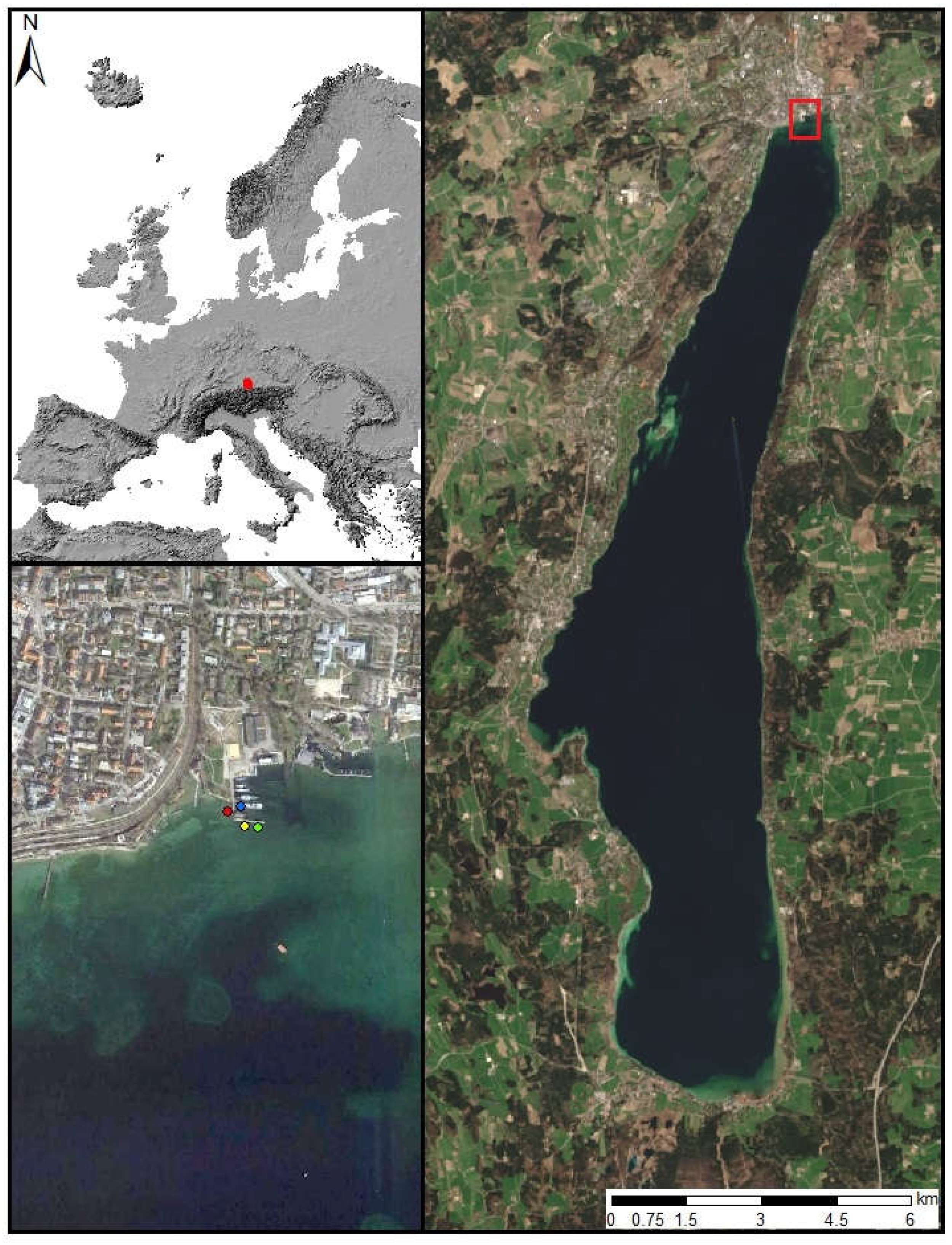
The study site is located in the northern part of Lake Starnberg near the town Starnberg (47.9° N, 11.3° E), situated 25 km south of Munich in Southern Germany (Figure 1). The current state of the lake is oligotrophic [47]. With a surface area of 56.4 km² and a maximum depth of about 127 m, Lake Starnberg is Germany’s fifth largest lake [48]. At this test site, populations of three coexisting macrophyte species were measured within the growing seasons of 2011 and 2015. The invasive species Elodea nuttallii as well as the two indigenous species Chara spp. and Potamogeton perfoliatus were investigated. The test site Chara is covered by Chara aspera (80%), Chara delicatula (10%) and Chara intermedia (10%). The 3 test sites are pure stands, one for each species. During both growing seasons, all measurements were taken at exactly the same positions. The water temperature of Lake Starnberg is continuously monitored by Bavarian Environmental Agency [49] every hour at the study site in the northern part of the lake.
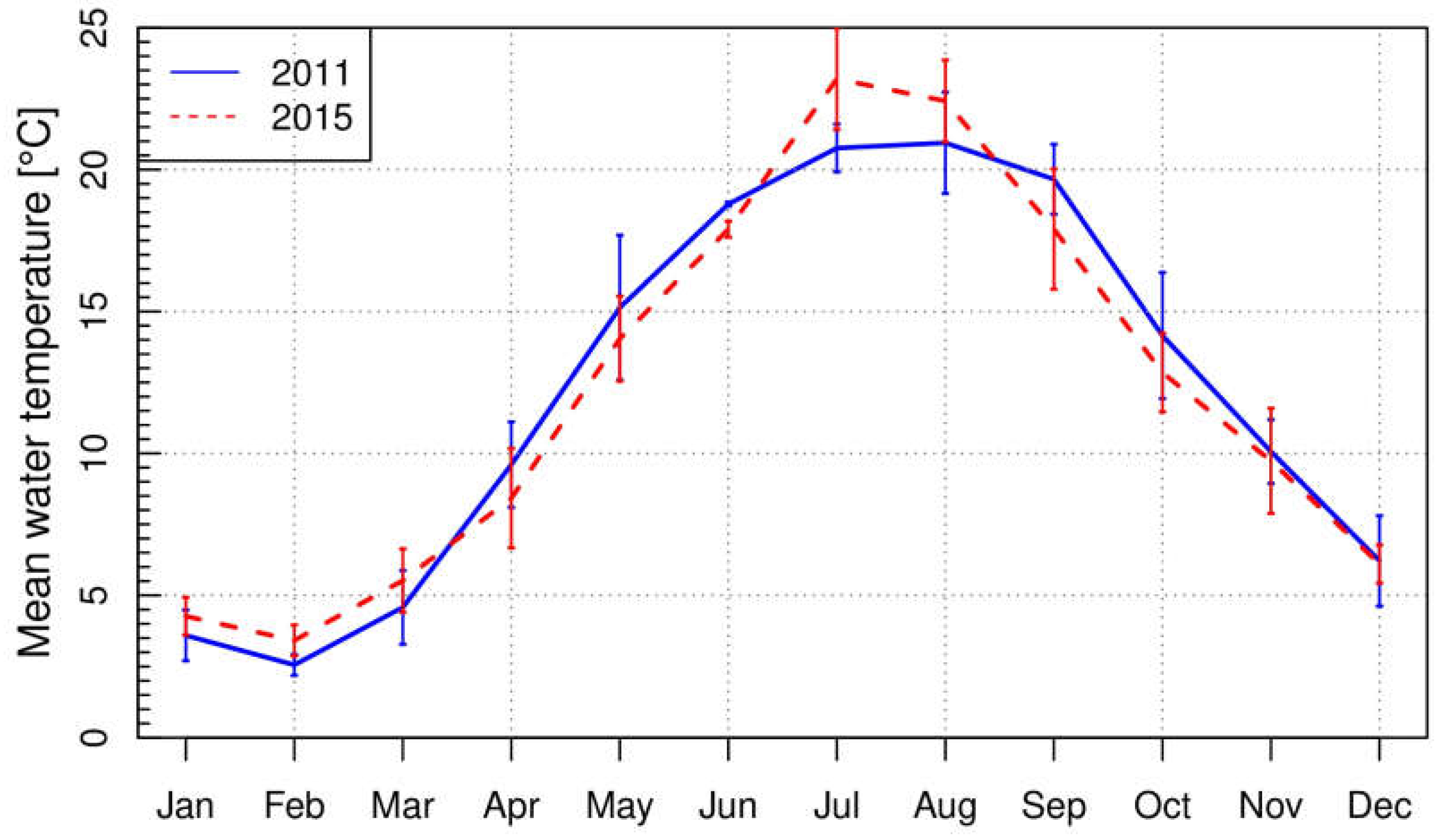
Monthly water temperatures of Lake Starnberg are displayed for 2011 and 2015 (Figure 2). In 2015, mean monthly water temperatures were higher in January (+0.7 °C), February (+0.9 °C), March (+0.9 °C), July (+2.4 °C) and August (+1.5 °C) compared to 2011. The remaining 7 months (April (−1.2 °C), May (−1.1 °C), June (−0.9 °C), September (−1.8 °C), October (−1.3 °C), November (−0.3 °C) and December (−0.1 °C)) had lower values than in 2011. In summary, the beginning of 2015 was warmer (January to March), while the spring temperatures were lower (April to June). During the main growing season in July and August, the temperatures in 2015 were higher. In contrast, 2011 had warmer autumn temperatures (September and October). Overall, the mean water temperature in 2015 was +0.05 °C higher.
2.2. In-Situ Measurements
During the growing seasons of 2011 and 2015, remote sensing reflectance spectra of pure stands of three macrophyte species were recorded systematically at the same study site and with the same measurement setup to cover different phenologic stages. The setup was performed on a jetty (Figure 3). With the aid of an extension arm a distance of 3 m between sensors and jetty was maintained. This stationary setup avoided drifting as well as shading and neighborhood effects due to an optimal sun-object-sensor geometry. The measurement setup consisted of three submersible RAMSES spectroradiometers (ACC-VIS and ARC-VIS; spectral range: 320 nm to 950 nm; TriOS Mess- und Datentechnik GmbH, Rastede, Germany) [50] and an underwater camera system (Canon PowerShot G10, Canon, Tokyo, Japan). The camera was used to monitor the sensor position and to document the bottom coverage of the measurement spot by live stream. The downwelling and upwelling hemispherical irradiance ( and ) as well as the upwelling radiance (with a field of view of 7°) were collected simultaneously within a range of 320 nm to 950 nm in 3.3 nm intervals. The data collection took place above sediment surface (depth b) before appearance of vegetation as well as just beneath the water surface (depth 0). During the plant growing period, the measurements at depth b were done above the macrophyte canopy. The distance between sensors and plant canopy respectively sediment was always 45 cm. The sensor depth in relation to the water surface was documented with a measuring tape fixed to the extension arm.
In both years, field campaigns were planned approximately every 3 weeks under cloud free conditions. The measurements at each single day were designed to start in the morning hours and to last until late afternoon. During the main growing season from mid-June to mid-September, sun position 1.5 h before and after noon in mid-September (Central European Time) was defined as the reference sun-zenith angle which should be captured by all daily measurement series. Under optimum conditions, up to 7 datasets per day and macrophyte patch were registered. The repetitions were conducted at the same places for each species. Each dataset consisted of 20 replicates within 3 min at the same fixed place and depths. For stable conditions, measurements in depth b and depth 0 were passed in quick succession.
2.3. Data Processing
The data processing chain was developed with Python (version 2.7.8, Python Software Foundation, Delaware, USA). For each dataset, the remote sensing reflectance spectra (b) and (0) of the two depths (depth b and 0) were calculated for 20 measurements of and [34]. Afterwards, the spectra were smoothed by Savitzky–Golay filter of length 5 [51]. For each of the 20 measurements of the dataset, the median was calculated. In line with Pinnel [38] and Wolf et al. [13] the spectra were cropped to a range of 400 to 700 nm to exclude strong sensor noise. (b) spectra above the canopy or sediment surface had to be corrected to eliminate the influence of the remaining water column of 45 cm between sensors and object. The water column correction was according to absorption models for phytoplankton [52] and colored dissolved organic matter [42], to backscattering models for phytoplankton [53] and non-algal particles [54], as well as absorption and backscattering coefficients of water and to the radiative transfer model of Albert and Mobley [55]. For calculating the required water constituent concentrations (Chl-a), colored dissolved organic matter (cDOM) and suspended particulate matter (SPM) were derived by an inversion of the diffuse vertical attenuation coefficient for downwelling irradiance as implemented in the water colour simulator WASI [56,57]. The attenuation coefficient was calculated with the method of Maritorena [58] by using measurements in two different depths (b and 0) at the same spot.
2.4. Reflectance Model
The corrected in-situ (b) spectra were used to create a model of remote sensing reflectance intensities. The reflectance model was a database model calculated in R (version 3.0.3, R Core Team, Vienna, Austria.) [59]. To cover the complete vegetation season as well as the differing sun heights, the collected remote sensing reflectance data had to be interpolated. A method for linear interpolation of irregular gridded data was applied (R package akima [60], R package stats [59]). The interpolation was carried out in two consecutive steps. First, a linear interpolation of the reflectance along the sun zenith angles for each measurement day was performed in steps of 1°. In the second step, reflectance intensities of the measurement days along the year were interpolated for each sun zenith angle separately. The model is limited to wavelengths from 400 nm to 700 nm and to sun zenith angles from 25° to 65°. Due to strong absorption of water in the near-infrared wavelengths the characteristic spectral features normally are superimposed by water absorption [41]. Hence, several surface models of reflectance intensities could be processed for each sun zenith angle. For each of the species sampled in the database, a spectrum can be produced together with confidence intervals.
2.5. Species-Specific Spectra
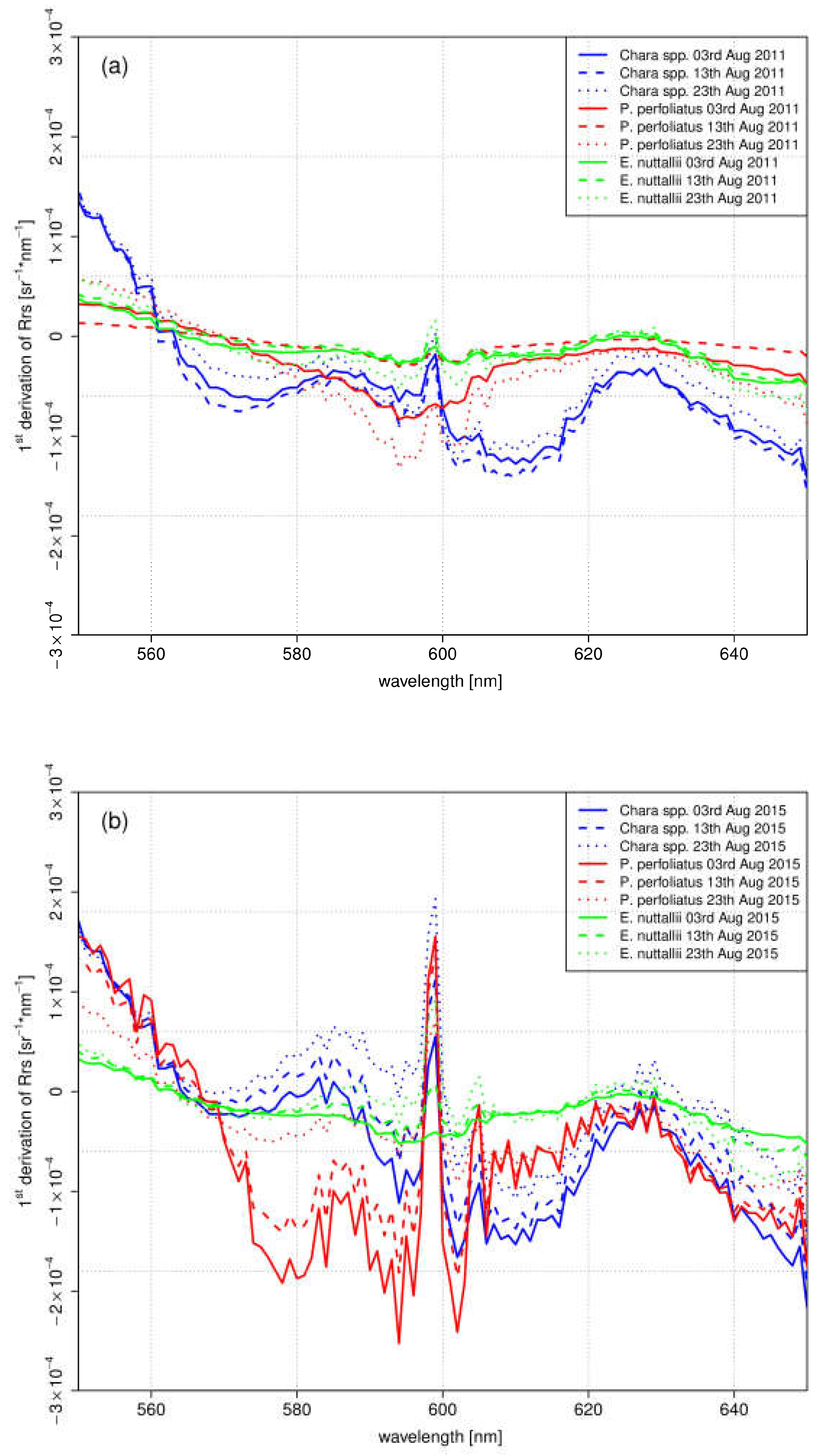
Out of the species-specific reflectance models, time series with an interval of 2 weeks and the same sun zenith angles were extracted for each species. The spectral responses on the appropriate dates of the investigated years were compared within the complete wavelength range. For the comparison of phenologic development of the different species, the 1st derivation of the spectra were calculated within the wavelengths 550 nm and 650 nm. The species were analyzed for August because for this month the vegetation maximum and the greatest temperature effects were expected.
2.6. Classification Process
The classification was based on the spectral libraries and was conducted with simulated spectra as derived from the reflectance model and followed a stepwise classification process chain [61] (Figure 4). For each classification level, a linear discriminant analysis was conducted and the spectrum was assigned to the best matching class. This procedure was conducted and repeated consecutively for each classification step. In the process, input spectra were adjusted to spectra in the spectral database with systematic measurements of 2010, 2011 and 2015 at Lake Starnberg. To facilitate the classification process, a pre-selection was conducted based on the date of the input spectra. The classification process was divided in four steps. Classification Step 1 was a separation in one of the categories: plant, sediment, plant/sediment, plant/water and water. Water and sediment were already final classes. Step 2 was assigning plant spectra of Step 1 to one of the macrophyte classes (Chara spp., E. nuttallii and P. perfoliatus). In Step 3 the species spectra were assigned to a phenologic stage. Step 4 was independent of Steps 2 and 3. In this step, input spectra classified as plant/sediment in Step 1 were attributed to defined species and phenologic stage. If the input spectrum was classified as plant/water in Step 1, this was assigned to tall growing species P. perfoliatus. Spectra with ambiguous phenologic stages were assigned to “no stage classifiable”. The validation of this classification method was performed with data from 2010 and 2011; the overall accuracies were calculated for each single classification step separately.
With this classification process chain, four main phenologic stages were distinguished. Stage 0 declares pure sediment, and Stage 1 sparsely vegetated sediment. Stage 2 describes a fully grown and upright standing vegetation. If the vegetation is already degrading and collapsing, it is classified as Stage 3. Differing subdivisions within one classification stage are attributed to varying bottom coverage and height of the macrophyte canopy.
3. Results
3.1. Reflectance Model
The reflectance models and the species-specific spectral response revealed clear differences between seasonal dates and phenologic stages. Spectral properties could be linked with diverse phenologic stages. A classification on species level and phenologic information revealed differences in accuracy for the different species. The highest accuracy was obtained for the test sites Chara (no misclassification on species level) and P. perfoliatus (two misclassifications on species level).
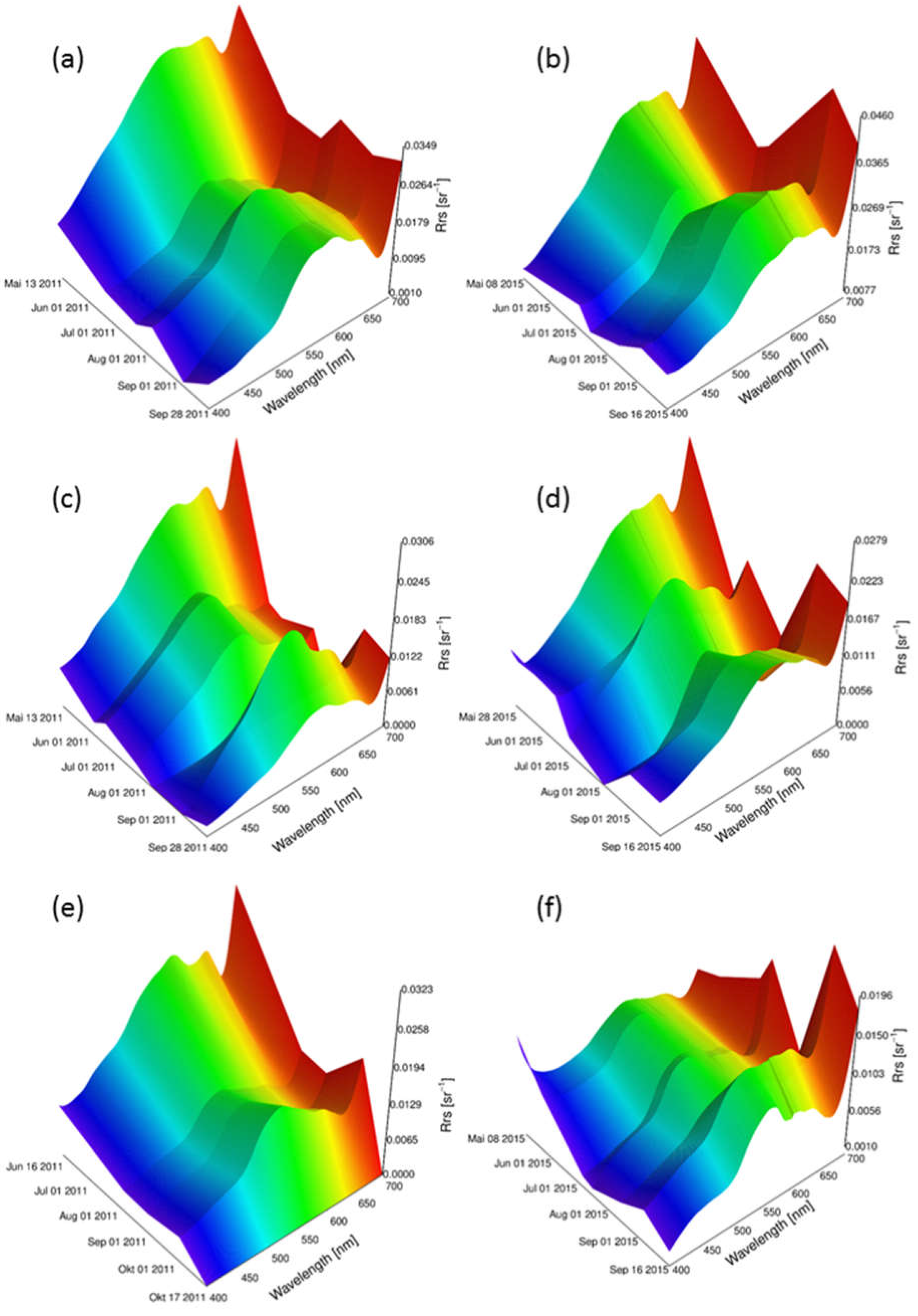
Reflectance models for 2011 and 2015 were simulated with linear interpolation method for the three macrophyte species Chara spp., E. nuttallii and P. perfoliatus separately (Figure 5). Depending on the first and last measurement day of the season, the models covered different time periods. For each species, the sun zenith angles were the same in both years. Variations of within a year could be observed. Overall, showed higher intensities at the beginning of the year. The intensities in the blue wavelength region (400 nm to 490 nm) were lower, the ones in green (490 nm to 560 nm) higher. A local reflectance minimum at around 680 nm could be observed for all sites and species. A difference in shape and intensity between both years and between the different species was obvious. However, a general trend could be observed for all species. The reflectance intensities decreased from May to August, followed by an increase towards the end of the growing season in September.
3.2. Species-Specific Spectra
spectra of different dates within the growing season of three macrophyte species were displayed side by side with top of view photographs of the test sites (Figure 6, Figure 7 and Figure 8). The spectra were simulated with the linear interpolation model. For 2011 and 2015, was plotted for same dates with in an interval of 10 days for the same sun zenith angle of each species. spectra covered wavelengths from 400 nm to 700 nm. The photos for documentation were recorded at the sampling days and do not show the situation at the day and daytime for which the spectra were simulated.
3.2.1. Test Site Chara
The simulated spectra of Chara spp. revealed the situation at a sun zenith angle of 35° in the afternoon from May (Figure 6a) to September (Figure 6e). In May (Figure 6a), the spectra of both years revealed a similar shape for the simulated days, differing in intensity. The intensity increased from 400 nm to 550 nm, followed by a plateau until 650 nm. Afterwards, intensity deceased, resulting in a local minimum at 680 nm. Within the year, the shape formed a maximum at about 570 nm, the minimum at 680 nm was more distinct (Figure 6b–d). Throughout August (Figure 6d), a difference in the phenologic development could be observed. Both shape and bottom coverage varied in the investigated years. The shape of 2015 clearly flattened in yellow and orange wavelength regions between 560 nm and 650 nm. This trend could be observed in September (Figure 6e) for both years.
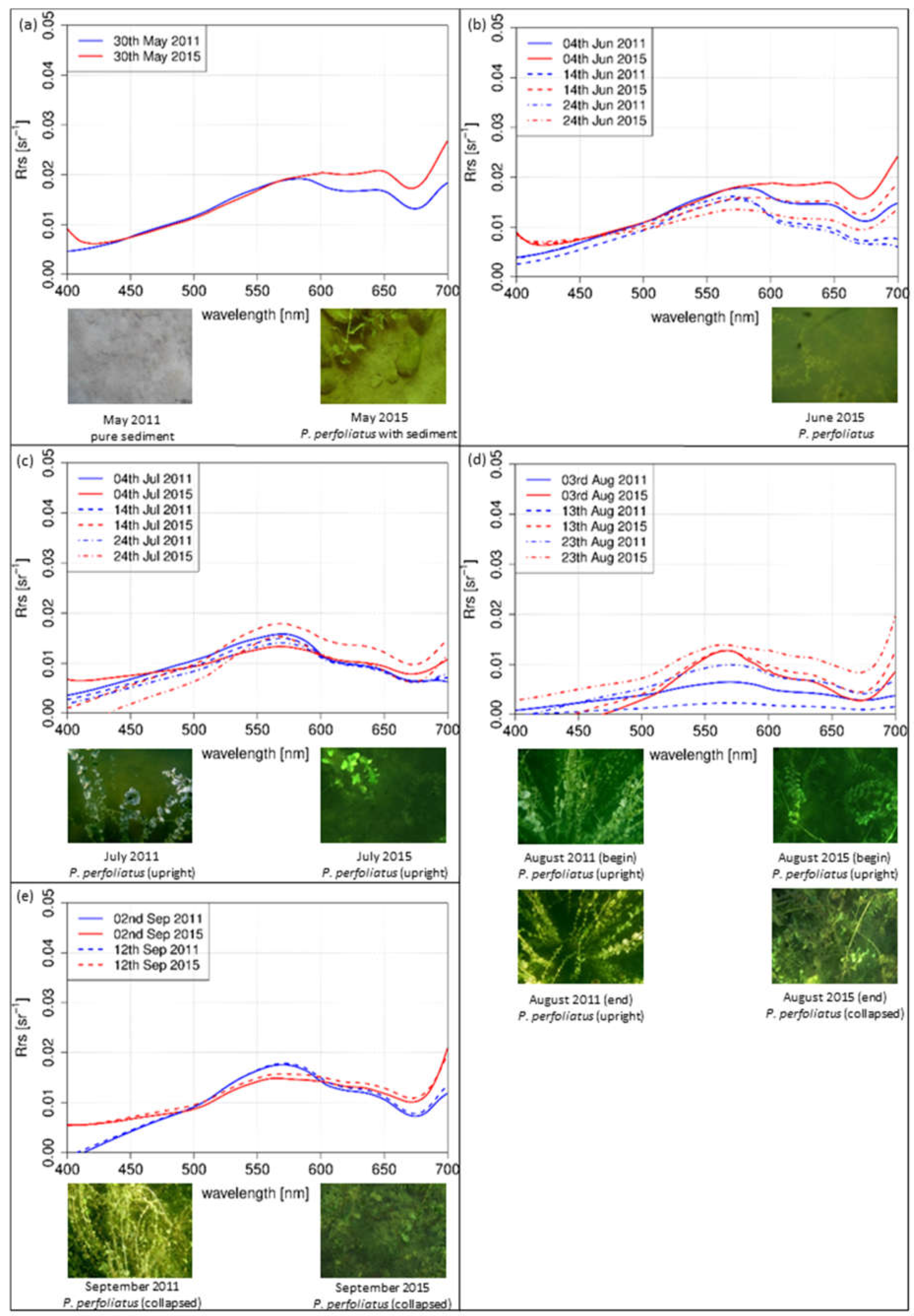
3.2.2. Test Site P. perfoliatus
The simulated spectra of P. perfoliatus were modeled with linear interpolation method and represented the situation from May (Figure 7a) to September (Figure 7e) at a sun zenith angle of 27° in the afternoon. In May (Figure 7a), the shapes of both years increased from 400 nm to 600 nm and a distinct local minimum at 680 nm was evident. In June (Figure 7b) and July (Figure 7c), a maximum at 570 nm was observed. In August (Figure 7d) and September (Figure 7e), differences in the species-specific development could be detected. In the investigated years, shape, bottom coverage and canopy structure varied. In August (Figure 7d), the maximum was evident in 2015. The shape of 2011 was flattened without a clear maximum. Flattened and compressed spectra in yellow and orange wavelengths (560 to 650 nm) were shown in 2015 in September (Figure 7e). The spectra of 2011 still revealed a distinct maximum in the green region.
3.2.3. Test Site E. nuttallii
The simulated spectra of E. nuttallii from May (Figure 8a) to September (Figure 8e) were calculated with linear interpolation method for a sun zenith angle of 31° in the afternoon. In May (Figure 8a), completely different shapes were evident for both years. The shape of the spectral curve in 2011 increased continuously. In June (Figure 8b), the spectra of 2011 displayed a continuous increase up to 560 nm followed by a plateau. Local minima were at 620 nm and 680 nm. In contrast, the simulated intensity of 2015 had a distinct maximum in the green region. In July (Figure 8c), the shapes in July were similar in both years, with a distinct maximum in the green wavelengths. Similar results were observed for August (Figure 8d), with a trend to flatten in the yellow and orange wavelength regions. In September (Figure 8e), the shapes were quite similar in both years with a distinct maximum in the green and lower intensity values in the blue and red regions, representing a vital and upright standing vegetation as confirmed by the photos.
3.2.4. Water Temperature Effect on Species-Specific Growth
The first derivation of in-situ spectra reflected the variations of the gradient between the investigated species within August (Figure 9). The species-specific variations differed in the different years. E. nuttallii showed slight variations of the gradient within months and between both years in this wavelength range. Clear differences between both years were observed for the indigenous species Chara spp. and P. perfoliatus. Overall, the gradient in 2011 was lower. The monthly variations of the gradient were higher in 2015, especially in the wavelength range between 570 nm and 610 nm. In this year, the mean water temperatures were higher during main growing season in July and August (Figure 2).
3.3. Spectral Classification on Species Level
The classification results revealed a continuous succession of phenologic stages for the test site Chara (Table 1). The overall accuracy of Step 1 was 70%, and of Step 2 82%. The accuracy of the assignment to a phenologic stage was between 79% (E. nuttallii) and 91% (Chara spp.).
The growing season is starting with sediment (2011) and plant/sediment (2015) spectra in May, followed by plant/sediment (2011) and plant (2015) spectra in June and July. In 2011, an interruption of the phenologic succession could be observed on 14 July, 24 July and 3 August. For the test site P. perfoliatus, a continuous succession of phenologic stages could be observed for both years. In 2011, the succession was interrupted on 3 and 13 August. The test site E. nuttallii showed several irregularities in both years. In 2011, one misclassification took place on 4 June. The other spectra were classified as plant/sediment or sediment consistently. Due to the small spectral differences, no classification on species level was possible at the test site E. nuttallii. In 2015, irregularities in the phenologic succession could be located on 4 June, 14 June and 24 July.
4. Discussion
The main research question, whether in-situ measured spectral variations within the growing season can be linked to phenologic stages of macrophyte populations, was confirmed by our results. An interrelation between macrophyte growth and water temperature was also demonstrated for the indigenous species Chara spp. and P. perfoliatus, but not for the invasive species E. nuttallii. The reflectance models developed based on the spectral signatures taken within the growing season and over the course of the day, proved to be able to mitigate gaps in in-situ data collection (e.g., due to cloud coverage). The models deliver simulated spectra for each day and all sun positions of possible optical satellite data takes (approximate ±2 h around noon). The inversion of the models for Chara spp. and P. perfoliatus with the aim of macrophyte classification on species level is successful. Restricting the search period based on external information about the weather history of that season and giving an estimate of the phenologic development stage additionally improve the classification success. Especially in that direction, we expect further advances by linking the modeling runs for species identification with external information on extreme events such as drought or rainy periods.
4.1. Phenologic Development in Spectra and Water Temperature
The general phenologic development scheme we observed is similar for the investigated species in both investigated years. Phenologic development stages control the changes in spectral response within the growing season [8,13]. Differing bottom coverage and species-specific structure elements like biomass, chlorophyll content, canopy height and alignment explain the variations of the shape of the spectra within the growing season. The species-specific phenologic development depends on the environmental conditions such as water temperature, water clarity, morphology and nutrient load [8,24,62]. To characterize the response of different macrophyte species to different environmental conditions, the species-specific spectral signatures within two growing seasons within two growing seasons is most informative. Water temperature was the only relevant variable available for both years. It is well-known that freshwater lakes buffer air temperature changes very well, which is explained by their thermal properties. The effects are smoothed and result in delayed water temperature effects. Nevertheless, these temperature fluctuations affect the biologic activities in the lake, affecting growth processes of submersed macrophytes as well.
In our discussion, we concentrate on August because the maximum of vegetation development is expected and greatest temperature effects (both acutely and accumulated) are expected at this time point. The most significant changes were observed in the green to red wavelength region, on which we concentrate in our analysis.
For the test sites Chara (Figure 6d,e) and P. perfoliatus (Figure 7d,e), the flattened shape of the spectral signature in the yellow and orange wavelength region is interpreted as a variation in leaf pigment ratio [13,63]. The intraspecific variations are illustrated by the derivation of the spectra for August (Figure 9). Especially, a lower Chl-a content in ageing leaves induces such a shift in yellow and orange wavelengths [63,64]. Higher water temperatures during the main growing season in July and August 2015 (Figure 2) may have resulted in a shortened growing season with earlier senescence [8,65]. The earlier senescence is demonstrated by a flattened shape (550 nm and 650 nm) with a slight gradient (Figure 9). The change in bottom coverage ratio (Figure 6e) and macrophyte structure (Figure 7d) confirms the assumption that water temperature influences the length of growing season. The pictures clearly show the decrease of plant covered area as well as collapsed and degraded macrophytes, with both phenomena being connected to macrophyte degradation.
In contrast to the indigenous species, the species-specific development of the invasive species E. nuttallii reveals spectral differences at the beginning of the growing season (Figure 8a,b). Higher water temperatures in the first quarter of 2015 (Figure 2) might explain induction of an earlier vegetation begin. During the main vegetation time in July and August, neither the spectral shape nor the bottom coverage are affected by higher water temperatures (Figure 9). This might be attributed to the better adaption to higher water temperatures of E. nuttallii [66].
The interpretation of the measurements of the indigenous species Chara spp. and P. perfoliatus indicate a shortened growing season at warmer temperatures in 2015. For the test site Chara, the shape of the spectra on 13 August 2015 (Figure 6d) and 2 September 2011 (Figure 6e) are almost the same. Consequently, the growing season and phenologic stage in 2015 was about 20 days shorter for Chara spp. than in 2011. This result coincides with higher water temperature during the main growing season in July and August 2015. The observations for P. perfoliatus in 2015 are similar. The spectral signature reflects the beginning of macrophyte degradation already at the end of August, visible by a flattened signature curve especially in the yellow to red region of the spectra. Such a phenologic shift at the end of the growing season was not found in E. nuttallii. A shortened growing season for indigenous species might be linked to higher water temperatures. E. nuttallii is probably not affected due to a higher temperature tolerance compared to the investigated indigenous species [66].
4.2. Reflectance Model
The developed reflectance models (Figure 5) provide species-specific spectral signatures throughout the complete growing season for every required sun position during a defined day. These protracted and detailed spectral pieces of information can strongly improve the knowledge of the seasonal variation of macrophyte species. The output spectra of these models provide a useful and necessary basis for bio-optical models such as BOMBER [54] or WASI [56,57].
The prediction limits are directly related to two variable groups: the daily and seasonal distribution of in-situ measurements and the specific environmental frame conditions of the respective year. In case of the distribution of in-situ measurements within the vegetation season there is a clear rule: the shorter the time-gaps between the in-situ measurements, the more detailed are the reflectance models. With high probability, the date of the vegetation maximum (e.g., maximum vegetation height and extension; highest biomass content) [8] is between two sampling days and cannot be expected to be represented by the model. In addition, for the applied linear interpolation method, an extrapolation for situations before and after the beginning and end of the measurements series is not possible.
Environmental parameters such as water clarity, water temperature and nutrient load affect macrophyte expansion and phenologic development [24,62]. Environmental parameters vary from year to year, affecting the prediction accuracy of the model outputs. The examined variable in this study, the water temperature, seems to trigger a variation in reflectance intensity and shape between the two investigated years (Figure 5a,c,e in contrast to Figure 5b,d,f). Further studies on the influence of light availability on the spectral variation might improve the accuracy of these reflectance models and the output spectra. In contrast, short-term events like draughts, floods or turbidity after an intense rainfall cannot directly be represented by the models. Such short-term and partial effects are highly different in different years. Due to the inertness and buffer action of freshwater lakes, these short-term events are attenuated and influence the models indirectly. We expect that this type of effects might be buffered and constrained by integration of external information into the inversion processes.
4.3. Model Inversion for Species Level Classification
The inversion of the reflection models with the aim of classifying macrophyte species and their phenologic stage for predefined daytimes and dates is successful. The inversion procedure delivers reliable spectra which we used for the comparison of phenologic development stages in 2011 and 2015. The analysis of the investigated macrophytes on species level (classification Step 2) based on phenologic development stages (Table 1) reveals an overall logic succession for the test sites Chara and P. perfoliatus for both investigated years.
The phenologic succession of Chara spp. was not accurately predicted for three dates in July and August 2011. The phenologic stage Chara spp. 1.1 induces a sediment proportion of 0.5 [61]. One explanation is a temporary sediment deposition masking the plant canopy. Sediment cover inevitably will result in an apparently higher sediment fraction and accordingly higher signal intensity [67].
In August 2011, a misclassification due to an interruption of the logic succession, on species level occurred for the test site P. perfoliatus. The in-situ measurement and classification of single growing plants without a closed plant canopy is more difficult and error-prone than for dense populations [68]. With the applied measurement setup, meadowy canopies such as Chara spp. allow a more stable spectral data collection resulting in a good to excellent classification success.
For the test site E. nuttallii, misclassification on species level occurred for 4 June in both years. A classification based on phenologic stages was not successful at all with the dataset for 2011. In 2015, the logic succession was interrupted. Slight water depth, shipping traffic, shading and a plant canopy up to the water surface hindered the in-situ data collection which might explain the misclassifications at this test site.
The accuracy of the classification results depends on the number of spectra of the spectral database. To obtain more detailed information about species composition and canopy structure, several in-situ measurements at different phenologic stages are required [44]. Spectral databases are able to provide day and daytime specific reference spectra of the lake bottom substrates. The knowledge of phenologic development related spectral response seems necessary when trying to improve the simulation and analysis of optical properties and light field parameters of deep and shallow waters in satellite datasets. This detailed information for the diverse phenologic stages of macrophytes are expected to improve the inversion success of bio-optical models such as BOMBER [54] and WASI [56,57]. Such models presently are the most sophisticated methods for deriving optical properties and light field parameters of deep and shallow waters from satellite data. Such information is required for the monitoring of freshwater lakes and large water bodies in general as e.g., included in the WFD. A further improvement of the prognosis accuracy of this evaluation chain is expected by steering the selection of the appropriated spectral signatures by e.g., detailed information about weather history of the respective growing season or the expected phenologic stage during data take.
5. Conclusions
Remote sensing methods offer a great potential to build up a monitoring system of submersed aquatic plants. A key requirement is the automatic discrimination of submersed macrophyte species. A spectral library with phenologic features as base for coupled growth and reflectance models seems essential for monitoring lake bottom substrates, especially for macrophytes. In the present study, the seasonal phenologic and spectral variability of aquatic plants at a test site at Lake Starnberg was investigated for 2011 and 2015. Water temperature was identified as one of the environmental driver explaining the phenologic shift by spectral signature analysis.
Investigations into the influence of the effects of small-scaled extreme weather conditions (e.g., light availability and turbidity) are highly recommended topics of future work. To improve the accuracy of the classification results, a large database is needed. Test sites are recommended in several lakes of diverse trophic states and on other macrophyte species, especially on potentially invasive species, to identify site-specific and species-specific variations of remote sensing reflectance. Further influences of the reflectance signal are related to periphyton coverage on macrophyte leaves.
Acknowledgments
This research was founded by the Federal Ministry for Economic Affairs and Energy (BMWi) under the grand number 50EE1336. We would like to thank our colleagues at Limnological Research Station Iffeldorf of Technical University of Munich for their support in fieldwork.
Author Contributions
Christine Fritz and Thomas Schneider conceived and designed the experiments; Christine Fritz performed the experiments; Christine Fritz and Thomas Schneider analyzed the data; and Christine Fritz, Thomas Schneider and Juergen Geist conceived, structured and jointly wrote the paper.
Conflicts of Interest
The authors declare no conflict of interest.
References
- Melzer, A. Aquatic macrophytes as tools for lake management. Hydrobiologia 1999, 396, 181–190. [Google Scholar] [CrossRef]
- Søndergaard, M.; Johansson, L.S.; Lauridsen, T.L.; Jørgensen, T.B.; Liboriussen, L.; Jeppesen, E. Submerged macrophytes as indicators of the ecological quality of lakes. Freshw. Biol. 2010, 55, 893–908. [Google Scholar] [CrossRef]
- Skubinna, J.P.; Coon, T.G.; Batterson, T.R. Increased abundance and depth of submersed macrophytes in response to decreased turbidity in saginaw bay, lake huron. J. Gt. Lakes Res. 1995, 21, 476–488. [Google Scholar] [CrossRef]
- Poikane, S.; Birk, S.; Böhmer, J.; Carvalho, L.; de Hoyos, C.; Gassner, H.; Hellsten, S.; Kelly, M.; Lyche Solheim, A.; Olin, M.; et al. A hitchhiker’s guide to european lake ecological assessment and intercalibration. Ecol. Indic. 2015, 52, 533–544. [Google Scholar] [CrossRef]
- Penning, W.E.; Dudley, B.; Mjelde, M.; Hellsten, S.; Hanganu, J.; Kolada, A.; van den Berg, M.; Poikane, S.; Phillips, G.; Willby, N.; et al. Using aquatic macrophyte community indices to define the ecological status of european lakes. Aquat. Ecol. 2008, 42, 253–264. [Google Scholar] [CrossRef]
- Silva, T.S.F.; Costa, M.P.F.; Melack, J.M.; Novo, E.M.L.M. Remote sensing of aquatic vegetation: Theory and applications. Environ. Monit. Assess. 2008, 140, 131–145. [Google Scholar] [CrossRef] [PubMed]
- Short, F.T.; Neckles, H.A. The effects of global climate change on seagrasses. Aquat. Bot. 1999, 63, 169–196. [Google Scholar] [CrossRef]
- Rooney, N.; Kalff, J. Inter-annual variation in submerged macrophyte community biomass and distribution: The influence of temperature and lake morphometry. Aquat. Bot. 2000, 68, 321–335. [Google Scholar] [CrossRef]
- European Commission. The Water Framework Directive (Directive 2000/60/ec of the European Parliament and of the Council of 23 October 2000 Establishing a Framework for Community Action in the Field of Water Policy); Official Journal of the European Communities: Brussels, Belgium, 2000; pp. 1–72. [Google Scholar]
- Palmer, S.C.J.; Kutser, T.; Hunter, P.D. Remote sensing of inland waters: Challenges, progress and future directions. Remote Sens. Environ. 2015, 157, 1–8. [Google Scholar] [CrossRef]
- Dörnhöfer, K.; Oppelt, N. Remote sensing for lake research and monitoring—Recent advances. Ecol. Indic. 2016, 64, 105–122. [Google Scholar] [CrossRef]
- Yuan, L.; Zhang, L.-Q. Mapping large-scale distribution of submerged aquatic vegetation coverage using remote sensing. Ecol. Inform. 2008, 3, 245–251. [Google Scholar] [CrossRef]
- Wolf, P.; Rößler, S.; Schneider, T.; Melzer, A. Collecting in situ remote sensing reflectances of submersed macrophytes to build up a spectral library for lake monitoring. Eur. J. Remote Sens. 2013, 46, 401–416. [Google Scholar] [CrossRef]
- Roessler, S.; Wolf, P.; Schneider, T.; Melzer, A. Multispectral remote sensing of invasive aquatic plants using rapideye. In Earth Observation of Global Changes (EOGC); Krisp, M.J., Meng, L., Pail, R., Stilla, U., Eds.; Springer Berlin Heidelberg: Berlin, Germany, 2013; pp. 109–123. [Google Scholar]
- Pinnel, N.; Heege, T.; Zimmermann, S. Spectral discrimination of submerged macrophytes in lakes using hyperspectral remote sensing data. SPIE Proc. Ocean Opt. XVII 2004, 1, 1–16. [Google Scholar]
- Malthus, T.J.; George, D.G. Airborne remote sensing of macrophytes in cefni reservoir, anglesey, UK. Aquat. Bot. 1997, 58, 317–332. [Google Scholar] [CrossRef]
- Giardino, C.; Bartoli, M.; Candiani, G.; Bresciani, M.; Pellegrini, L. Recent changes in macrophyte colonisation patterns: An imaging spectrometry-based evaluation of southern Lake Garda (Northern Italy). APPRES 2007, 1, 011509–011517. [Google Scholar]
- George, D.G. The airborne remote sensing of phytoplankton chlorophyll in the lakes and tarns of the english lake district. Int. J. Remote Sens. 1997, 18, 1961–1975. [Google Scholar] [CrossRef]
- Dekker, A.G.; Vos, R.J.; Peters, S.W.M. Analytical algorithms for lake water TSM estimation for retrospective analyses of TM and SPOT sensor data. Int. J. Remote Sens. 2002, 23, 15–35. [Google Scholar] [CrossRef]
- Malthus, T.J.; Karpouzli, E. Integrating field and high spatial resolution satellite-based methods for monitoring shallow submersed aquatic habitats in the Sound of Eriskay, Scotland, UK. Int. J. Remote Sens. 2003, 24, 2585–2593. [Google Scholar] [CrossRef]
- Barko, J.W.; Gunnison, D.; Carpenter, S.R. Sediment interactions with submersed macrophyte growth and community dynamics. Aquat. Bot. 1991, 41, 41–65. [Google Scholar] [CrossRef]
- Squires, M.M.; Lesack, L.F. Spatial and temporal patterns of light attenuation among lakes of the mackenzie delta. Freshw. Biol. 2003, 48, 1–20. [Google Scholar] [CrossRef]
- Barko, J.W.; Smart, R.M. Sediment-related mechanisms of growth limitation in submersed macrophytes. Ecology 1986, 67, 1328–1340. [Google Scholar] [CrossRef]
- Shuchman, R.A.; Sayers, M.J.; Brooks, C.N. Mapping and monitoring the extent of submerged aquatic vegetation in the laurentian great lakes with multi-scale satellite remote sensing. J. Gt. Lakes Res. 2013, 39, 78–89. [Google Scholar] [CrossRef]
- Singh, S.P.; Singh, P. Effect of temperature and light on the growth of algae species: A review. Renew. Sustain. Energy Rev. 2015, 50, 431–444. [Google Scholar] [CrossRef]
- Zhu, B.; Mayer, C.M.; Rudstam, L.G.; Mills, E.L.; Ritchie, M.E. A comparison of irradiance and phosphorus effects on the growth of three submerged macrophytes. Aquat. Bot. 2008, 88, 358–362. [Google Scholar] [CrossRef]
- Madsen, T.V.; Brix, H. Growth, photosynthesis and acclimation by two submerged macrophytes in relation to temperature. Oecologia 1997, 110, 320–327. [Google Scholar] [CrossRef] [PubMed]
- Hoffmann, M.A.; Raeder, U.; Melzer, A. Influence of environmental conditions on the regenerative capacity and the survivability of elodea nuttallii fragments. J. Limnol. 2014, 74. [Google Scholar] [CrossRef]
- Hoffmann, M.; Raeder, U. Predicting the potential distribution of neophytes in southern Germany using native Najas marina as invasion risk indicator. Environ. Earth Sci. 2016, 75, 1217. [Google Scholar] [CrossRef]
- Hoffmann, M.; Sacher, M.; Lehner, S.; Raeder, U.; Melzer, A. Influence of sediment on the growth of the invasive macrophyte Najas marina ssp intermedia in lakes. Limnologica 2013, 43, 265–271. [Google Scholar] [CrossRef]
- Morel, A.; Belanger, S. Improved detection of turbid waters from ocean color sensors information. Remote Sens. Environ. 2006, 102, 237–249. [Google Scholar] [CrossRef]
- Mertes, L.A.K.; Smith, M.O.; Adams, J.B. Estimating suspended sediment concentrations in surface waters of the Amazon River wetlands from Landsat images. Remote Sens. Environ. 1993, 43, 281–301. [Google Scholar] [CrossRef]
- Bostater, J.C.R.; Ghir, T.; Bassetti, L.; Hall, C.; Reyeier, E.; Lowers, R.; Holloway-Adkins, K.; Virnstein, R. Hyperspectral Remote Sensing Protocol Development for Submerged Aquatic Vegetation in Shallow Waters; SPIE: Bellingham, WA, USA, 2004; pp. 199–215. [Google Scholar]
- Mobley, C.D. Estimation of the remote-sensing reflectance from above-surface measurements. Appl. Opt. 1999, 38, 7442–7455. [Google Scholar] [CrossRef] [PubMed]
- Mumby, P.J.; Clark, C.D.; Green, E.P.; Edwards, A.J. Benefits of water column correction and contextual editing for mapping coral reefs. Int. J. Remote Sens. 1998, 19, 203–210. [Google Scholar] [CrossRef]
- Heblinski, J.; Schmieder, K.; Heege, T.; Agyemang, T.K.; Sayadyan, H.; Vardanyan, L. High-resolution satellite remote sensing of littoral vegetation of lake sevan (armenia) as a basis for monitoring and assessment. Hydrobiologia 2011, 661, 97–111. [Google Scholar] [CrossRef]
- Fritz, C.; Doernhoefer, K.; Schneider, T.; Geist, J.; Oppelt, N. Mapping submerged aquatic vegetation using rapideye satellite data: The example of Lake Kummerow (Germany). Water 2017, 9, 510. [Google Scholar] [CrossRef]
- Pinnel, N. A Method for Mapping Submerged Macrophytes in Lakes Using Hyperspectral Remote Sensing. Ph.D. Thesis, Technische Universität München, München, Germany, 2007. [Google Scholar]
- Williams, D.J.; Rybicki, N.B.; Lombana, A.V.; O’Brien, T.M.; Gomez, R.B. Preliminary investigation of submerged aquatic vegetation mapping using hyperspectral remote sensing. Environ. Monit. Assess. 2003, 81, 383–392. [Google Scholar] [CrossRef]
- Fyfe, S. Spatial and temporal variation in spectral reflectance: Are seagrass species spectrally distinct? Limnol. Oceanogr. 2003, 48, 464–479. [Google Scholar] [CrossRef]
- Armstrong, R.A. Remote sensing of submerged vegetation canopies for biomass estimation. Int. J. Remote Sens. 1993, 14, 621–627. [Google Scholar] [CrossRef]
- Gitelson, A.A.; Zur, Y.; Chivkunova, O.B.; Merzlyak, M.N. Assessing carotenoid content in plant leaves with reflectance spectroscopy. Photochem. Photobiol. 2002, 75, 272–281. [Google Scholar] [CrossRef]
- Gausman, H.W. Evaluation of factors causing reflectance differences between sun and shade leaves. Remote Sens. Environ. 1984, 15, 177–181. [Google Scholar] [CrossRef]
- Hestir, E.L.; Khanna, S.; Andrew, M.E.; Santos, M.J.; Viers, J.H.; Greenberg, J.A.; Rajapakse, S.S.; Ustin, S.L. Identification of invasive vegetation using hyperspectral remote sensing in the California delta ecosystem. Remote Sens. Environ. 2008, 112, 4034–4047. [Google Scholar] [CrossRef]
- Elatawneh, A.; Kalaitzidis, C.; Petropoulos, G.P.; Schneider, T. Evaluation of diverse classification approaches for land use/cover mapping in a mediterranean region utilizing hyperion data. Int. J. Digit. Earth 2014, 7, 194–216. [Google Scholar] [CrossRef]
- Stoffels, J.; Hill, J.; Sachtleber, T.; Mader, S.; Buddenbaum, H.; Stern, O.; Langshausen, J.; Dietz, J.; Ontrup, G. Satellite-based derivation of high-resolution forest information layers for operational forest management. Forests 2015, 6, 1982–2013. [Google Scholar] [CrossRef]
- Arle, J.; Blondzik, K.; Claussen, U.; Duffek, A.; Grimm, S.; Hilliges, F.; Hoffmann, A.; Leujak, W.; Mohaupt, V.; Naumann, S.; et al. Wasserwirtschaft in Deutschland. Teil 2. Gewässergüte; Umweltbundesamt (UBA): Bonn, Germany, 2013. (In Germany) [Google Scholar]
- Wöbbecke, K.; Klett, G.; Rechenberg, B. Wasserbeschaffenheit der Wichtigsten Seen in der Bundesrepublik Deutschland: Datensammlung 1981–2000; Umweltbundesamt: Dessau-Roßlau, Germany, 2003. (In Germany) [Google Scholar]
- Bavarian Environmental Agency. Bavarian Hyrological Service. Available online: http://www.Gkd.Bayern.De (accessed on 13 July 2017).
- TriOS. Ramses Radiometer. Available online: http://www.Trios.De/en/products/sensors/ramses.html (accessed on 13 July 2017).
- Savitzky, A.; Golay, M.J.E. Smoothing and differentiation of data by simplified least squares procedures. Anal. Chem. 1964, 36, 1627–1639. [Google Scholar] [CrossRef]
- Bricaud, A.; Babin, M.; Morel, A.; Claustre, H. Variability in the chlorophyll-specific absorption coefficients of natural phytoplankton: Analysis and parameterization. J. Geophys. Res. 1995, 100, 13321. [Google Scholar] [CrossRef]
- Brando, V.E.; Dekker, A.G. Satellite hyperspectral remote sensing for estimating estuarine and coastal water quality. IEEE Trans. Geosci. Remote Sens. 2003, 41, 1376–1387. [Google Scholar] [CrossRef]
- Giardino, C.; Candiani, G.; Bresciani, M.; Lee, Z.; Gagliano, S.; Pepe, M. Bomber: A tool for estimating water quality and bottom properties from remote sensing images. Comput. Geosci. 2012, 45, 313–318. [Google Scholar] [CrossRef]
- Albert, A.; Mobley, C.D. An analytical model for subsurface irradiance and remote sensing reflectance in deep and shallow case-2 waters. Opt. Express 2003, 11, 2873–2890. [Google Scholar] [CrossRef] [PubMed]
- Gege, P. Wasi-2d: A software tool for regionally optimized analysis of imaging spectrometer data from deep and shallow waters. Comput. Geosci. 2013, 62, 208–215. [Google Scholar] [CrossRef]
- Gege, P. The water color simulator wasi: An integrating software tool for analysis and simulation of optical in situ spectra. Comput. Geosci. 2004, 30, 523–532. [Google Scholar] [CrossRef]
- Maritorena, S. Remote sensing of the water attenuation in coral reefs: A case study in french polynesia. Int. J. Remote Sens. 1996, 17, 155–166. [Google Scholar] [CrossRef]
- R Core Team. R: A Language and Environment for Statistical Computing; R Foundation for Statistical Computing: Vienna, Austria, 2014; Available online: http://www.R-project.org/ (accessed on 13 July 2017).
- Akima, H.; Gebhardt, A.; Petzoldt, T.; Maechler, M. Akima: Interpolation of Irregularly Spaced Data, R package version 0.5-11; Available online: https://cran.r-project.org/web/packages/akima/index.html (accessed on 13 July 2017).
- Wolf, P.K.-H. In Situ-Messungen als Basis Für Wachstums-/Reflexionsmodelle Submerser Makrophyten. Ph.D. Thesis, Technische Universität München, München, Germany, 2014. (In Germany). [Google Scholar]
- Blindow, I. Long- and short-term dynamics of submerged macrophytes in two shallow eutrophk lakes. Freshw. Biol. 1992, 28, 15–27. [Google Scholar] [CrossRef]
- Sims, D.A.; Gamon, J.A. Relationships between leaf pigment content and spectral reflectance across a wide range of species, leaf structures and developmental stages. Remote Sens. Environ. 2002, 81, 337–354. [Google Scholar] [CrossRef]
- Gitelson, A.; Merzlyak, M.N. Quantitative estimation of chlorophyll-a using reflectance spectra: Experiments with autumn chestnut and maple leaves. J. Photochem. Photobiol. B Biol. 1994, 22, 247–252. [Google Scholar] [CrossRef]
- Barko, J.W.; Smart, R.M. Comparative influences of light and temperature on the growth and metabolism of selected submersed freshwater macrophytes. Ecol. Monogr. 1981, 51, 219–235. [Google Scholar] [CrossRef]
- McKee, D.; Hatton, K.; Eaton, J.W.; Atkinson, D.; Atherton, A.; Harvey, I.; Moss, B. Effects of simulated climate warming on macrophytes in freshwater microcosm communities. Aquat. Bot. 2002, 74, 71–83. [Google Scholar] [CrossRef]
- Wolter, P.T.; Johnston, C.A.; Niemi, G.J. Mapping submergent aquatic vegetation in the US great lakes using quickbird satellite data. Int. J. Remote Sens. 2005, 26, 5255–5274. [Google Scholar] [CrossRef]
- Sawaya, K.E.; Olmanson, L.G.; Heinert, N.J.; Brezonik, P.L.; Bauer, M.E. Extending satellite remote sensing to local scales: Land and water resource monitoring using high-resolution imagery. Remote Sens. Environ. 2003, 88, 144–156. [Google Scholar] [CrossRef]
Figure 1.
Study site at Lake Starnberg. Measurement points of macrophyte test sites (red: Chara, blue: E. nuttallii, green: P. perfoliatus) and water temperature (yellow) (Google Earth Imagery, Image 2017 Landsat/Copernicus). Landsat 8 true-color composite (acquisition date: 7 April 2014; data source: USGS).

Figure 2.
Monthly mean water temperature and standard deviation at Lake Starnberg in 2011 and 2015.

Figure 3.
Measurement setup of in-situ data collection (modified from Wolf et al. [13]).
Figure 3.
Measurement setup of in-situ data collection (modified from Wolf et al. [13]).
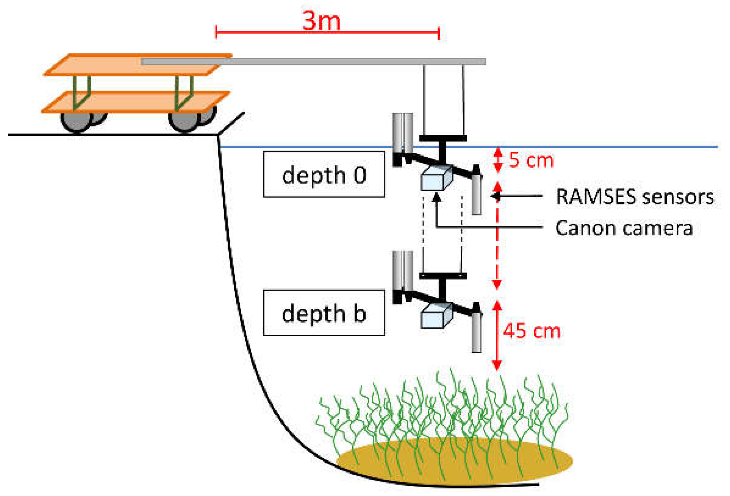
Figure 4.
Schematic diagram of the stepwise classification after Wolf [60].
Figure 4.
Schematic diagram of the stepwise classification after Wolf [60].
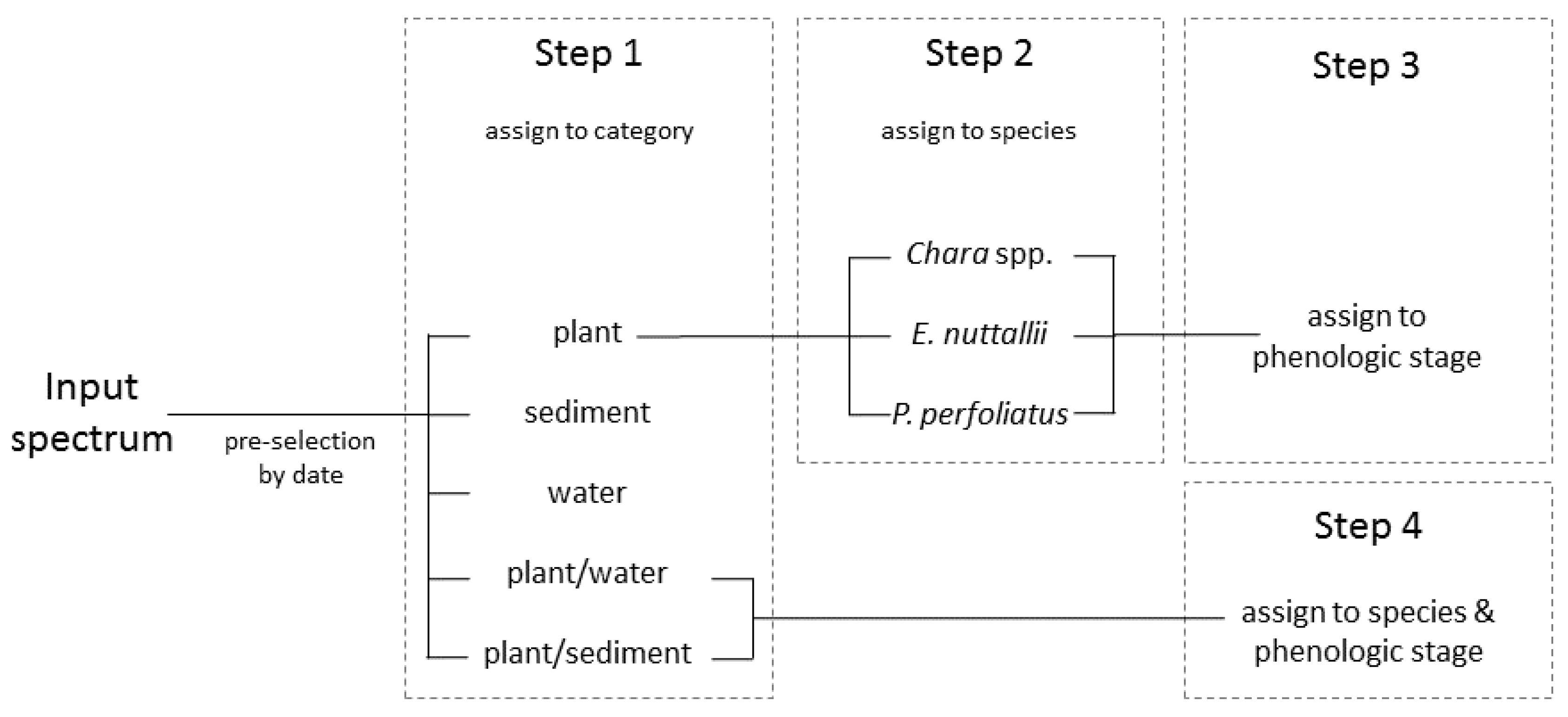
Figure 5.
Reflectance models of three macrophyte species for 2011 and 2015. Chara spp. for sun zenith angle 35° in: (a) 2011; and (b) 2015; P. perfoliatus for sun zenith angle 27° in: (c) 2011; and (d) 2015; and E. nuttallii for sun zenith angle 31° in: (e) 2011; and (f) 2015.
Figure 5.
Reflectance models of three macrophyte species for 2011 and 2015. Chara spp. for sun zenith angle 35° in: (a) 2011; and (b) 2015; P. perfoliatus for sun zenith angle 27° in: (c) 2011; and (d) 2015; and E. nuttallii for sun zenith angle 31° in: (e) 2011; and (f) 2015.

Figure 6.
Simulated intensities of Chara spp. modeled with a linear interpolation method of 2011 (blue) and 2015 (red). Top view photos of the investigated test sites of the sampling days: (a) May; (b) June; (c) July; (d) August; and (e) September.
Figure 6.
Simulated intensities of Chara spp. modeled with a linear interpolation method of 2011 (blue) and 2015 (red). Top view photos of the investigated test sites of the sampling days: (a) May; (b) June; (c) July; (d) August; and (e) September.
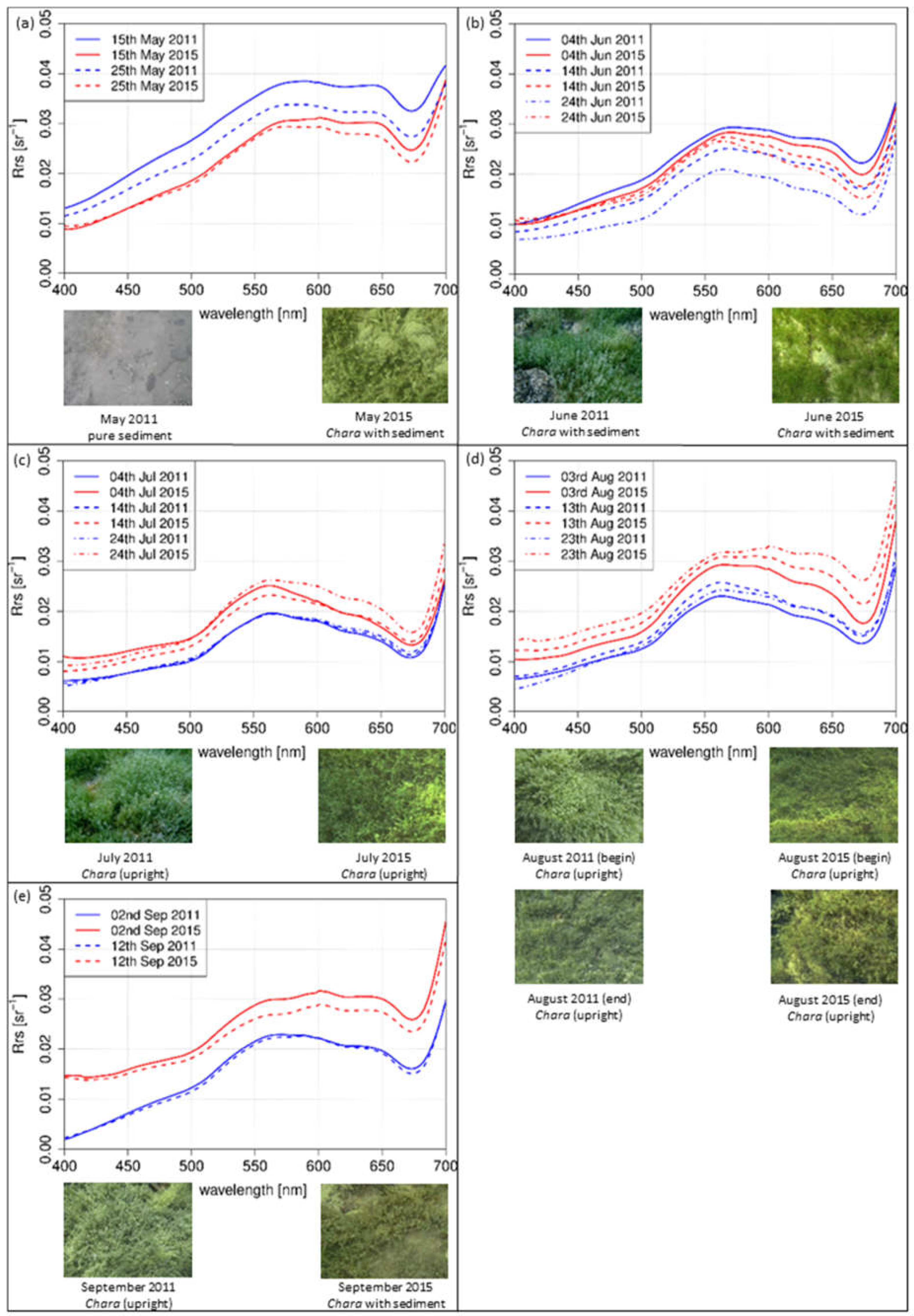
Figure 7.
Simulated intensities of P. perfoliatus modeled with a linear interpolation method of 2011 (blue) and 2015 (red). Top view photos of the investigated test sites of the sampling days: (a) May; (b) June; (c) July; (d) August; and (e) September.
Figure 7.
Simulated intensities of P. perfoliatus modeled with a linear interpolation method of 2011 (blue) and 2015 (red). Top view photos of the investigated test sites of the sampling days: (a) May; (b) June; (c) July; (d) August; and (e) September.

Figure 8.
Simulated intensities of E. nuttallii modeled with a linear interpolation method of 2011 (blue) and 2015 (red). Top view photos of the investigated test sites of the sampling days: (a) May; (b) June; (c) July; (d) August; and (e) September.
Figure 8.
Simulated intensities of E. nuttallii modeled with a linear interpolation method of 2011 (blue) and 2015 (red). Top view photos of the investigated test sites of the sampling days: (a) May; (b) June; (c) July; (d) August; and (e) September.
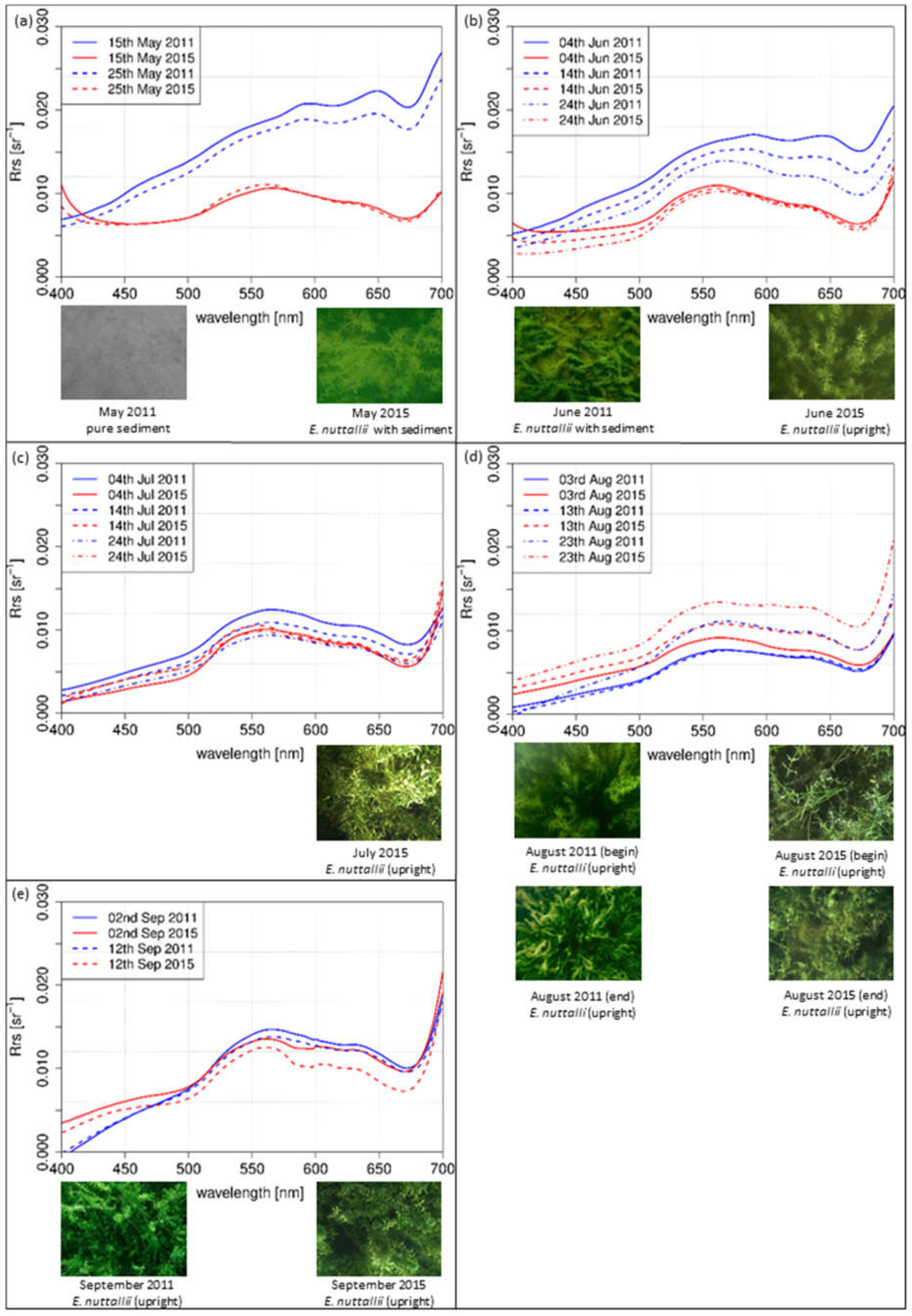
Figure 9.
1st Derivation of in-situ spectra of: August 2011 (a); and August 2015 (b), in a wavelength range between 550 nm and 650 nm.
Figure 9.
1st Derivation of in-situ spectra of: August 2011 (a); and August 2015 (b), in a wavelength range between 550 nm and 650 nm.

Table 1.
Results of the stepwise classification after Wolf [60] for Chara spp., E. nuttallii and P. perfoliatus.
Table 1.
Results of the stepwise classification after Wolf [60] for Chara spp., E. nuttallii and P. perfoliatus.
| Date | Test site Chara 2011 | Test Site Chara 2015 | Test Site P. perfoliatus 2011 | Test Site P. perfoliatus 2015 | Test Site E. nuttallii 2011 | Test Site E. nuttallii 2015 | |
|---|---|---|---|---|---|---|---|
| 15 May | 100% sediment | 100% plant/sediment 100% Chara spp. 1.1 | - | - | 100% sediment | 99.99% plant 100% E. nuttallii 100% E. nuttallii 2.1 | |
| 25 May | 100% sediment | 100% plant/sediment 100% Chara spp. 1.2 | 30 May 100% sediment | 30 May 100% sediment | 100% sediment | 100% plant 100% E. nuttallii 100% E. nuttallii 2.1 | |
| 4 June | 100% sediment | 100% plant/sediment 100% Chara spp. 1.2 | 100% plant/water 100% P. perfoliatus 1 | 100% sediment | 100% plant/sediment 100% Chara spp. 1.2 | 100% plant/water 100% P. perfoliatus 1 | |
| 14 June | 100% plant/sediment 100% Chara spp. 1.2 | 100% plant/sediment 100% Chara spp. 1.2 | 100% plant/water 100% P. perfoliatus 1 | 100% plant/water 100% P. perfoliatus 1 | 100% plant/sediment no stage classifiable | 100% plant/sediment no stage classifiable | |
| 24 June | 100% plant/sediment 100% Chara spp. 1.2 | 100% plant 100% Chara spp. 100% Chara spp. 2 | 100% plant/water 100% P. perfoliatus 1 | 100% plant/water 100% P. perfoliatus 1 | 100% plant/sediment no stage classifiable | 100% plant 100% E. nuttallii 100% E. nuttallii 2.2 | |
| 4 July | 100% plant/sediment 100% Chara spp. 1.2 | 100% plant 100% Chara spp. 100% Chara spp. 2 | 100% plant/water 100% P. perfoliatus 1 | 100% plant/water 100% P. perfoliatus 1 | 100% plant/sediment no stage classifiable | 100% plant 100% E. nuttallii 100% E. nuttallii 2.2 | |
| 14 July | 100% plant/sediment 100% Chara spp. 1.1 | 100% plant 100% Chara spp. 100% Chara spp. 2 | 100% plant 100% P. perfoliatus 100% P. perfoliatus 2 | 100% plant/water 100% P. perfoliatus 1 | 100% plant/sediment no stage classifiable | 100% plant 100% E. nuttallii 100% E. nuttallii 2.2 | |
| 24 July | 100% plant/sediment 100% Chara spp. 1.1 | 100% plant 100% Chara spp. 100% Chara spp. 2 | 100% plant 100% P. perfoliatus 100% P. perfoliatus 2 | 100% plant/water 100% P. perfoliatus 1 | 99.99% plant/sediment no stage classifiable | 100% plant 100% E. nuttallii 100% E. nuttallii 3 | |
| 3 August | 99.91% plant/sediment 100% Chara spp. 1.1 | 100% plant 100% Chara spp. 100% Chara spp. 2 | 100% plant99.48% E. nuttallii 100% E. nuttallii 2.3 | 100% plant 100% P. perfoliatus 100% P. perfoliatus 2 | 99.82% plant/sediment no stage classifiable | 100% plant 100% E. nuttallii 100% E. nuttallii 2.3 | |
| 13 August | 89.58% plant/sediment no stage classifiable | 99.99% plant 100% Chara spp. 100% Chara spp. 2 | 99.99% plant 100% E. nuttallii 100% E. nuttallii 2.3 | 100% plant 100% P. perfoliatus 100% P. perfoliatus 2 | 99.99% plant/sediment no stage classifiable | 99.99% plant 100% E. nuttallii 100% E. nuttallii 2.3 | |
| 23 August | 99.90% plant/sediment no stage classifiable | 100% plant 100% Chara spp. 100% Chara spp. 3.1 | 99.99% plant 99.98% P. perfoliatus 100% P. perfoliatus 3.1 | 100% plant 100% P. perfoliatus 100% P. perfoliatus 3.1 | 100% plant/sediment no stage classifiable | 99.99% plant 100% E. nuttallii 100% E. nuttallii 2.3 | |
| 2 September | 100% plant/sediment no stage classifiable | 99.99% plant 100% Chara 100% Chara 3.1 | 100% plant 100% P. perfoliatus 100% P. perfoliatus 3.1 | 100% plant 100% P. perfoliatus 100% P. perfoliatus 3.1 | 100% plant/sediment no stage classifiable | 100% plant 100% E. nuttallii 100% E. nuttallii 2.3 | |
| 12 September | 100% plant/sediment no stage classifiable | 100% plant/sediment no stage classifiable | 100% plant 100% P. perfoliatus 100% P. perfoliatus 3.1 | 100% plant/water no stage classifiable | 100% plant/sediment no stage classifiable | 100% plant 100% E. nuttallii 100% E. nuttallii 2.3 | |
© 2017 by the authors. Licensee MDPI, Basel, Switzerland. This article is an open access article distributed under the terms and conditions of the Creative Commons Attribution (CC BY) license (http://creativecommons.org/licenses/by/4.0/).
Share and Cite
MDPI and ACS Style
Fritz, C.; Schneider, T.; Geist, J. Seasonal Variation in Spectral Response of Submerged Aquatic Macrophytes: A Case Study at Lake Starnberg (Germany). Water 2017, 9, 527. https://doi.org/10.3390/w9070527
AMA Style
Fritz C, Schneider T, Geist J. Seasonal Variation in Spectral Response of Submerged Aquatic Macrophytes: A Case Study at Lake Starnberg (Germany). Water. 2017; 9(7):527. https://doi.org/10.3390/w9070527
Chicago/Turabian StyleFritz, Christine, Thomas Schneider, and Juergen Geist. 2017. "Seasonal Variation in Spectral Response of Submerged Aquatic Macrophytes: A Case Study at Lake Starnberg (Germany)" Water 9, no. 7: 527. https://doi.org/10.3390/w9070527
Note that from the first issue of 2016, this journal uses article numbers instead of page numbers. See further details here.