The Limits of Water Pricing in a Developing Country Metropolis: Empirical Lessons from an Industrial City of Pakistan

Abstract

This paper seeks to question the effectiveness of water pricing as a means of consumer behavioural change in urban centres of the Global South by analysing the domestic usage for water in a major industrial city of Pakistan. Using survey data of 1100 households from Faisalabad city, we estimate the price and income elasticities of water demand. Instrumental variable methods are applied to overcome the endogeneity issues of water pricing. The findings reflect that price and income elasticities vary across different groups. Price elasticities range from −0.43 to −0.71, and income elasticities vary between 0.01 and 0.12. These findings suggest that pricing policies may have limited scope to drive households’ water consumption patterns. However, these empirics may suggest that policy makers should design an appropriate tariff structure to increase revenues that can be invested to further improve the existing water infrastructure. The study findings also suggest that non-pricing instruments, such as water saving campaigns, may be helpful in driving an efficient use of water in rapidly growing cities in the developing world.

1. Introduction

Urban water supply management has become a growing concern in many developing economies. Effective strategies to meet the water and sanitation targets of the United Nations Sustainable Development Goals (SDG 6) by 2030 will require us to develop a fast data-gathering capacity and an effective policy response to water demand challenges. The trends reflect continued water demand and supply imbalances, and a compromise on quality and the equitable distribution of water, in the wake of the growing population of cities. The formulation and implementation of effective water management policies has become imperative for ensuring efficient water delivery to urban areas, which is essential for socioeconomic development [1]. The provision of clean water safeguards or even improves public health by preventing water-borne diseases, thus saving financial and natural capital resources. Policy makers need evidence-based recommendations to justify cost effective supply options that ensure adequate water supply for growing urban populations. It is desirable to know which pricing or non-pricing policies are effective, and to what extent, to cater to the increasing water needs of growing populations through efficient water supply management in developing economies.

The literature on residential demand for drinking water in developing countries has been growing over the past few decades; however, there is no consensus on analytical methods yet. One of the reasons is the complex estimation of demand for drinking water, as households in these countries use multiple sources for drinking water [2]. Most of the existing studies analysed tariff structures along with other factors to guide the pricing policies in those countries [3,4]. A better understanding of household water use in developing countries is necessary for the efficient and effective management and expansion of water systems. The analysis of the pricing structure and income elasticities is critically important in formulating policies for improved water supply, particularly in the urban areas of developing economies.

The inefficient use of water in urban areas is a key concern in developing countries such as Pakistan. Identifying inefficiencies in water supply, usage, and other affiliated environmental and health related issues can help prompt policy responses and decision-making regarding efficient water supply to urban households. Moreover, international development best practices suggest that a state or local authority should be responsible for the delivery of safe drinking water to local residents [5]. Water pricing is an important economic instrument that not only supports improved infrastructure development (through increased revenues) but is also helpful in demand management policies to conserve and make efficient the use of water resources [6]. Pakistan is facing rapid urbanization, with a likelihood of half its population living in cities by 2025 [7]. The fast growing urban population in the country is posing many challenges, and mounting pressure on existing public services and infrastructure; particularly, drinking water demand and supply management. The situation becomes even more complex with the emergence of informal, unplanned, and underserviced settlements—slums—and the resultant overcrowding of cities. The provision and management of water for growing cities has become a principal policy concern for decision-makers.

Faisalabad is among the fastest urbanizing large cities of the country, and is also an agro-industrial and textile hub of Pakistan, making it an engine of growth for the national economy. The public and private sectors provide water from alternate sources at different prices. However, access to quality water is a serious problem in this fast growing city due to ground water contamination [8].

This study analyses pricing structures for improving water resource management and allocation in a major industrial urban centre of Pakistan. The paper contributes to the literature by estimating the demand elasticities of filtered and unfiltered water consumption, which have great policy relevance in devising pricing structures for urban water utilities. The survey data of 1100 households are used to estimate price and income elasticities. The results show that price elasticities of demand remain inelastic, but vary across all water consumer groups, suggesting that price adjustment policies may have little impact on water consumption patterns. Similarly, income elasticities turn out to be significantly positive, but remain small in magnitude. This implies that policy makers may consider a mix of instruments to affect water consumption patterns. Moreover, the findings also suggest that non-pricing measures can be helpful to deal with water scarcity issues.

The remainder of the paper is organized as follows. Section 2 provides an overview of the water management policies and the supply and tariff structure of the Water and Sanitation Authority (WASA), Faisalabad. This section also underscores the water supply efficiency issues of different components of WASA. Furthermore, it highlights the key issues related to water quality and delivery to households. Section 3 reviews the existing literature on household demand for drinking water and various approaches available to estimate price and income elasticities. Section 4 describes the data and empirical methods employed for the demand analysis. Section 5 discusses the empirical results of the demand and income elasticities and other factors explaining the demand for drinking water. Finally, Section 6 concludes with the policy recommendations of the study.

2. A Brief Overview of Water Management Policy in Faisalabad

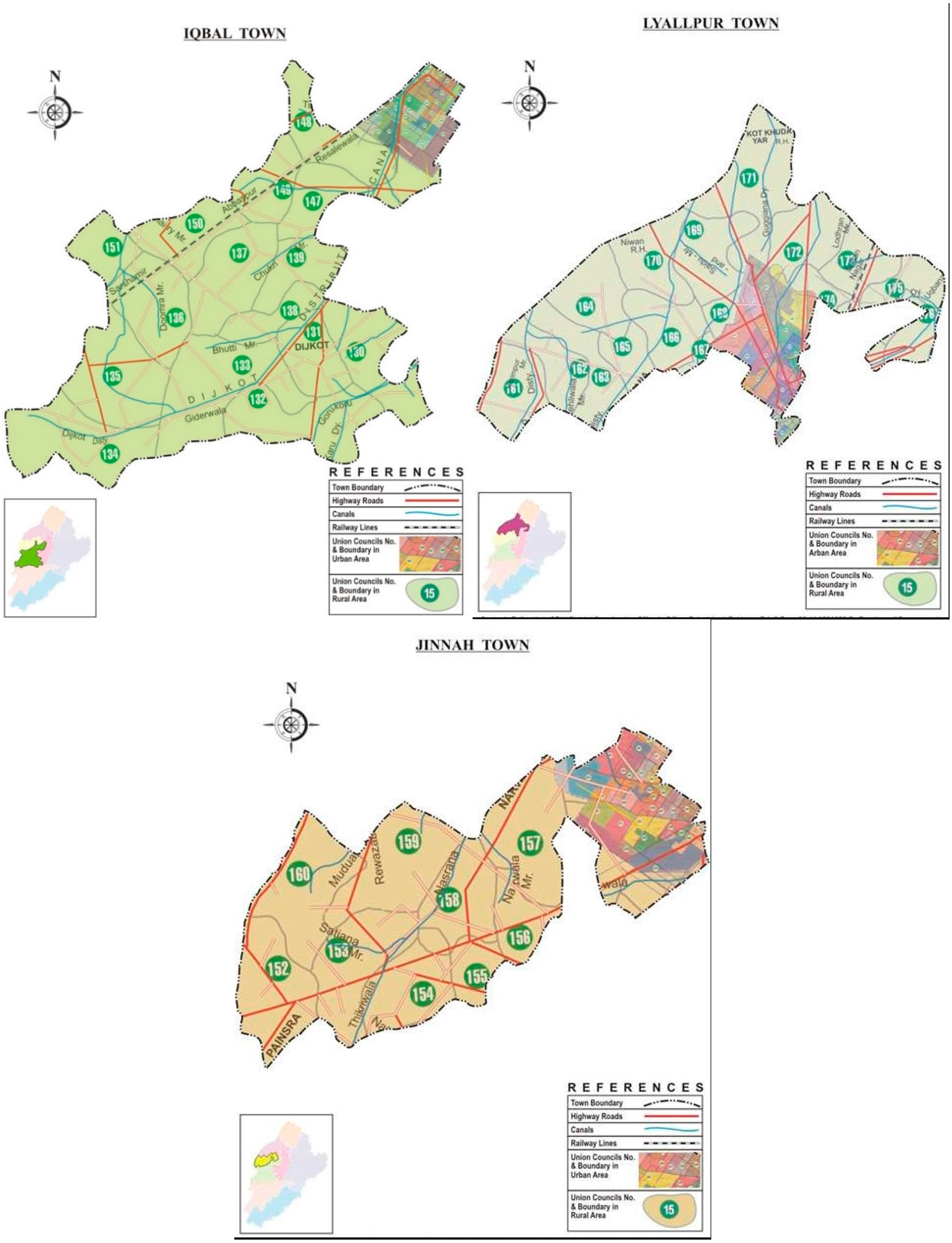
Faisalabad is the third largest city of Pakistan, with an estimated total population (including suburbs) of around 5.43 million as per Strategic Development Plan 2006–2011 and a projected figure of 8.79 million in 2023 [9] (the official number was 2.318 million during 1998 census [10] thus, reflects the high growth rate during the last decade). According to Pakistan Bureau of Statistics, the average household size for Faisalabad city is 7.2 [11]. The Faisalabad city government have setup municipal administration offices in each town (Further details in

Table A1. Urban population in Faisalabad (Census 1998).

Areas	Population	Urban Union Council	Household Number
Iqbal Town	783,173	22	108,774
Jinnah Town	765,700	30	106,347
Lyallpur Town	717,710	28	99,682
Madina Town	797,873	33	110,816
Total	3,064,456	113	425,619

Source: Extracted from City District Government Faisalabad website [11].

,

Table A2. Summary statistics of variables.

Variables	Sample Size	Mean	Standard Deviation
Quantities
Combined	1100	273.97	261.98
Filtered	519	123.98	200.37
Unfiltered	619	285.65	294.46
Prices
Combined	1191	1.21	1.29
Filtered	570	1.25	1.54
Unfiltered	581	1.18	1.00
Income	1100	33,966.67	21,127.89
Age	1100	39.78	12.11
Education	1100	9.99	4.85
Tank Water	49	0.10	0.29
Pipe Dummy	121	0.54	0.50
Filter Dummy	519	0.48	0.50

Source: Authors calculations from sample data.

). In 2005, District Faisalabad was divided into eight towns or administrative units, with a Town Municipal Administration (TMA) for each town (City District Government Faisalabad, details in Figure A1, Figure A2). However four out of eight towns constitute Faisalabad city or the urban core including, Iqbal Town, Jinnah Town, Lyallpur Town and Madina Town [11].

2.1. Water Market in Faisalabad

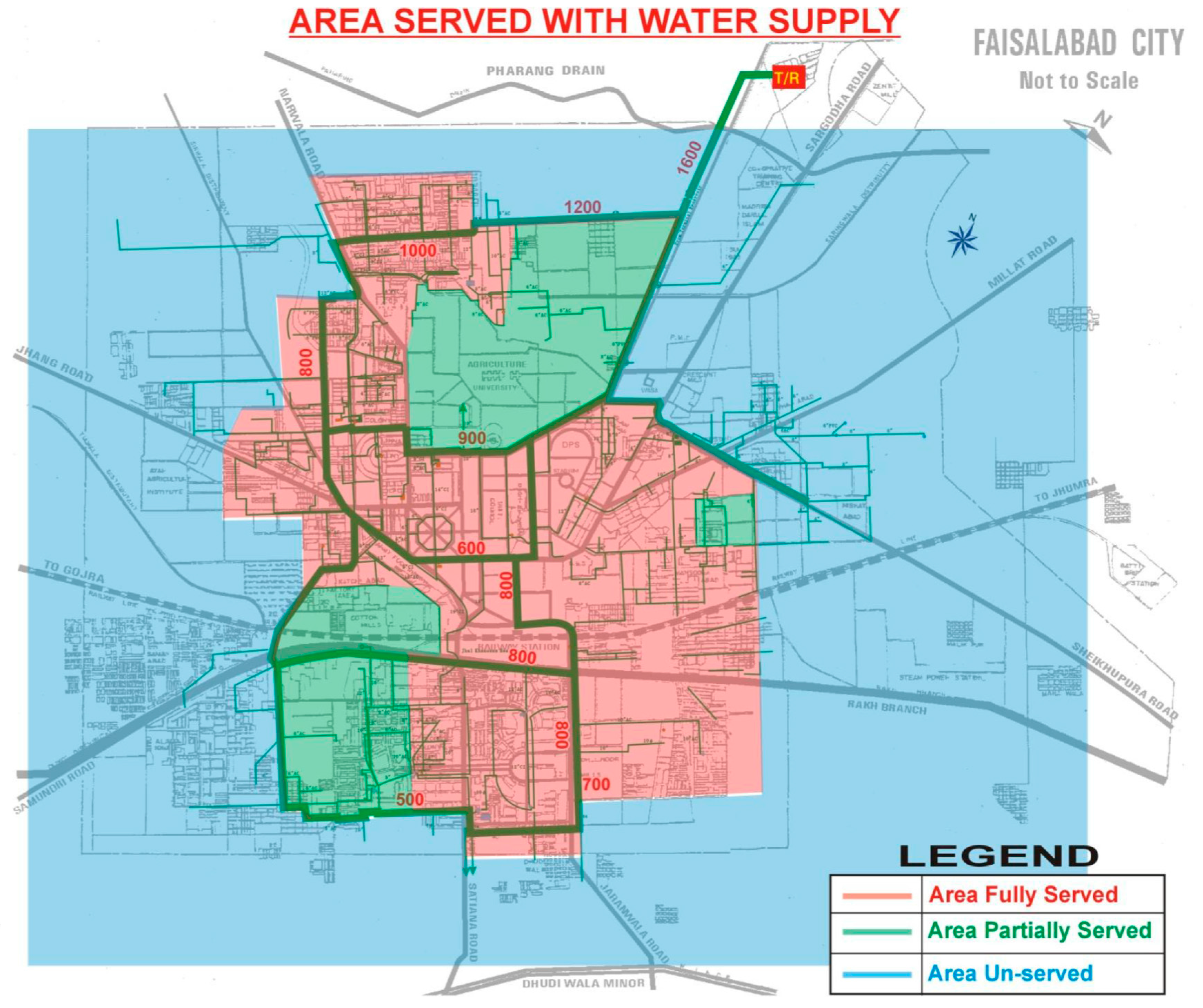
The Water and Sanitation Authority (WASA), established in 1978, is responsible for the provision of water and sewerage facilities to local residents of Faisalabad city. WASA, with its existing production capacity of 65 million gallons per day (with 260,000 available water pipeline connections), is able to connect only 60% of the households with direct water supply facilities and 72% with sewage facilities, based on their demographic estimates of Faisalabad’s core urban population of 3.2 million [12]. Figure 1 depicts the areas served by WASA for partial or full water supply. The groundwater in the city is mostly brackish. Therefore, most of the water is pumped from wells near the Chenab River for subsequent supply to the city.

Besides WASA, there is a range of private water supply sources in Faisalabad. These range from unfiltered canal-side pumped water to filtered bottled water. Many private sector providers supply filtered water and non-filtered sweet groundwater pumped from canal-side areas. Various sources of water supply in Faisalabad include: (i) canal-side pumped water; (ii) bottled water, such as Nestle, Aquafina, and Gourmet; (iii) unfiltered sweet water; (iv) small-scale filtration plants; (v) large commercial filtration plants; (vi) government filtration plants; (vii) groundwater bore; and (viii) tankers.

2.2. The Tariff Structure

WASA water consumption charges depend on the house size, and vary from PKR 83 (2.5 Marla house) per month to PKR 966 (40 Marla) per month. In addition, it charges a one-time water connection fee of PKR 483, PKR 3220, and PKR 3200 for residential, commercial, and industrial usage, respectively (PKR is local currency abbreviation for Pakistan Rupees). The current tariff plan of WASA is effective from 2006. In the fiscal year 2010–2011, WASA collected total revenues of PKR 735.03 million [12]. However, a low recovery rate of water bills has been a major challenge for WASA. The city government is spending a large amount of money for the provision of free filtered water. Moreover, the price charged for the pipe water connection is substantially lower than the market price due to high subsidies. WASA neither charges an aquifer fee for extraction of groundwater for domestic use, nor does it limit water usage, which might have created inefficiencies in the water market. As a result, a large proportion of households in Faisalabad have installed domestic borings to extract groundwater. They can thus consume unlimited water extracted from these borings, consequently leading to water scarcity issues.

2.3. Water Quality and Contamination Issues

Faisalabad faces enduring water quality issues. The groundwater in the majority of the areas of Faisalabad is contaminated and is not suitable for drinking. Diseases like diarrhea, dehydration, hepatitis, nausea, food poisoning, and other water borne diseases are at their highest incidence in Faisalabad [8]. According to WASA officials, the water is filtered at its source and is of sufficiently good quality. However, it becomes contaminated in transit. A variety of contaminants infiltrate the water due to pipe leakage and exposure to sewerage lines. A degraded water infrastructure and the inability of WASA to cover operations and maintenance costs have resulted in the supply of contaminated water. Piped water supplied by WASA is largely considered unfiltered.

3. Review of Existing Literature

Water pricing has been a longstanding development planning issue. Researchers have proposed various approaches to analyse different tariff structures by estimating price and income elasticities [13]. Although there is a vast literature focusing on household demand for water in developed economies, until the 1970s most of the studies on residential water demand had been mainly devoted to the United States, where some regions had been affected by periods of severe drought [14,15,16]. In the 1980s, many studies on residential water demand focused on an economic analysis using econometrics methods [17,18,19,20]. In the 1990s, researchers emphasized new insights, such as the adoption of low-flow equipment by households, the welfare consequences of price regulation, and case studies of European countries [21,22,23,24,25]. In the 2000s, researchers considered the importance of threshold price levels [26]. In general, price elasticity remains inelastic, and estimates vary between −0.10 and −0.30 [27,28]. For example, Strand and Walker [29] used household survey data from 17 cities in Central America and Venezuela to estimate the price elasticities for piped and non-piped households, which range from −0.3 to −0.1, respectively. Using the same dataset, Nauges and Strand [30] analysed the water demand for non-piped households in four cities of El Salvador and Honduras. Their results show that the non-tap water demand elasticities range between −0.4 and −0.7. Using cross-sectional household-level data from seven provincial Cambodian towns, Basani et al. [31] noted that the price elasticity of water demand for connected households was in the range of −0.4 and −0.5.

Despite the fact that water demand analysis in developing economies started a long time ago [32], the literature on these countries has been limited in the past. The empirical analysis of the water demand function in developing countries is less focused because of the unavailability of data, as water consumption is not always metered. Moreover, the use of multiple sources by different household groups makes water demand estimation even more complex, which needs careful investigation to draw appropriate inferences for policy making [2]. Therefore, well designed surveys are required to collect quality household-level data. Particularly, data on the conditions of access to different water sources (such as filtered vs. unfiltered water, distance to the source of water, time to commute the water, and the mode to commute the water) as well as on the quality and reliability are important [33].

Researchers have investigated the different factors preventing households from accessing water from different sources. For instance, McPhail [34] addressed the question of why households do not connect to a piped water system, using a survey in rural areas of Tunis and Tunisia. The survey results indicated that households cannot afford to pay for piped connections. Persson [35] analysed the choice of households in Philippines for drinking water sources. They argue that the demand for clean water for drinking purposes is derived demand, as it is an input to produce health. The results indicated that time cost (price coefficient) has a significant effect on choice probabilities. The results also indicated that the tastes of households have an insignificant effect on choice probabilities.

Similarly, Nauges and van den Berg [4] have used 1800 Sri Lankan households’ data to estimate the demand for piped and non-piped water sources. They argued that water supply service in many developing countries is at a very low level for residential consumers. They simultaneously estimated the substitutability/complementarity between piped and non-piped water sources, using a system of equations. The results of their study showed that the price elasticity of demand for piped water consumers is −0.15, whereas households relying on piped water as well as other sources to supplement their water consumption have a higher demand elasticity (−0.37). They also found evidence of substitutability between water from different sources. Wang et al. [36] analysed the willingness to pay for water, using a multiple bounded discrete choice (MBDC) survey model, with a survey of 1500 households in five suburban districts in the Chongqing Municipality. They showed that a significant increase in water price is economically feasible, as long as the poorest households are properly subsidized.

There are mixed findings about the demand and income elasticities of water in developing economies, which have different important policy implications for water management bodies in these countries. However, empirical findings related to household’s decisions for water sources are less robust, which need some rigorous analysis to obtain robust and reliable demand elasticity estimates [2].

The precise and accurate estimation of price and income elasticities would inform policy makers about how and to what extent these results can be helpful to devise viable water demand management policies. The efficient water pricing structure would not only reduce the loss of public water supply, but also encourage efficient production and consumption and ensure sustainable availability in the long run. However, it is difficult to obtain robust empirical findings in the presence of diverse water consumer groups. This paper analyses the demand elasticities and impact of other explanatory variables on water consumption for different water user groups in the urban dwellings of Faisalabad city. We apply an instrumental variable approach and bootstrapping methods to estimate water demand elasticities. This is the first study of such a kind in Pakistan, and it suggests important policy recommendations for urban water management authorities in Pakistan. It also provides useful insights for developing economies in general.

4. Methods and Data

4.1. Methodology

Conventionally, the demand function of a representative household is specified as $Q=f(P,X).$ Here, $Q$ represents the household water consumption, $P$ the price of water, and $X,$ is a vector of other exogenous variables (such as household income, age, and geographic factors). The linear estimation form can be described as

$$Q_i=X_i^{\prime }\beta +P_i\alpha +{\epsilon }_i$$

(1)

where $Q_i$ is the vector of $K\times 1$ quantities; $P_i$ the vector of $K\times 1$ prices; $X_i$ is a vector of exogenous variables (as stated above); and ${\epsilon }_i$ represents the vector of the $K\times 1$ random error term, ${\epsilon }_i\sim N(0,{\sigma }^2)$. $\alpha$ and $\beta$ are the vectors of the respective parameters of price and exogenous vectors. Generally, this type of linear demand function is directly estimated using the ordinary least square (OLS) method to obtain price and income elasticities [31,37,38]. However, the price $P_i$ is potentially correlated with the error term ${\epsilon }_i$ such that $E(P_i{\epsilon }_i)\ne 0$. There may be several possible factors (such as various water supply sources and unobservable individuals’ characteristics) causing price endogeneity, which leads to biased price elasticity estimates (see for details, Nauges and Thomas, 2000; Nauges and Whittington, 2010). This endogeneity problem can be resolved by introducing some instruments, which are correlated with price but uncorrelated with the error tem. To overcome this endogeneity issue we assume another variable $Z_i$ that is correlated with $P_i$ but uncorrelated with ${\epsilon }_i$. This variable can be used as an instrument such that

$$P_i=Z_i^{\prime }\gamma +{\upsilon }_i$$

(2)

where $Z_i$ is a vector of $m\times 1$, $\gamma$ is vector of the parameters, and ${\upsilon }_i$ is a vector of the error term. There can be several factors (instruments) that can cause a shift in water supply (i.e., a cost shifter) to identify the household demand for water of individual i. To ensure the identification of the casual effect of $\alpha$ from Equation (1), we assume (i) $E(Z_i{\epsilon }_i)=0;$ and (ii) $E(Z_i{P}_i)\ne 0.$ Now, in the presence of an instrumental variable, we can obtain unbiased estimates of the casual effect of $P_i$ on $Q_i$.

4.2. Empirical Setup

Most of the existing literature on water demand estimation relies on the ordinary least square (OLS) method for the separate estimation of the demand function for different water sources, which may produce biased estimates in the presence of endogenous water prices [3,37]. Some studies also apply maximum likelihood estimation methods to analyse water demand using multinomial logistic and probit models [30,35] while others use either two stage least square methods [29], or systems of demand equations [4].

We use an instrumental variable approach to estimate the price and income elasticities of residential demand for water from different sources in Faisalabad. For this, we consider a number of instruments which are expected to the shift the supply curve. These instruments are: (i) the cost of water supply in the winter and summer seasons; (ii) water leakages; (iii) tanker water delivery; and (iv) locality. For instance, we use the cost of water (in different seasons) as a proxy for a water supply shifter. Similarly, the locality variable is also an important instrument, as the allocation of water (from different sources) among different socio-economic areas (e.g., slums vs. high income areas) varies significantly, which will cause the shift in water supply.

In addition to pricing, water demand also varies considerably due to other factors, including household structure (e.g., size) and household characteristics (e.g., age, education); therefore, these factors needs to be accounted for in effective water demand management. The inclusion of socioeconomic and demographic characteristics allows us to capture consumers’ preferences in the water demand analysis. There is the possibility that price has more than one instrument, therefore, we need to test the validity of all of those instruments.

We include three different demand specifications in our model. First, we estimate a combined demand function to create baseline estimates of demand and income elasticities, along with other exogenous factors influencing the household water demand. In the case of Faisalabad, the quality of water is a significant factor affecting consumer preferences and water usage [39]. We also estimate a subsample of demand for filtered and unfiltered water. The estimable model is described as

$$\ln q_i^r={\alpha }_0+{\alpha }_1\ln p_i+{\beta }_k{\displaystyle \sum _{k=1}^K\ln x_{ki}}+{\delta }_m{\displaystyle \sum _{m=1}^M{D}_{mi}+{\epsilon }_i}$$

(3)

where, $q_i^r$ represents the quantities of water consumed by an individual household from different sources (such that $r=\mathrm{combined}, \mathrm{filtered} \mathrm{and} \mathrm{unfiltered} \mathrm{water} \mathrm{consumption}$); $p_i$ is defined as above; $x_{ki}$ represents the vector of household characteristics and other factors affecting the water demand, which include income, age, education, distance from water facility, and tank water; and $D_{mi}$ represents dummy variables for piped connection, house storeys, and filtered water consumption, respectively.

Since our primary goal is to estimate the price and income elasticities for different types of water consumption (e.g., filtered vs. unfiltered users), we can obtain those estimates directly by taking the partial derivatives of Equation (3) with respect to respective prices and individuals’ income, as

$${\zeta }^r=\frac{\partial \ln q^r}{\partial \ln p}={\alpha }^r \mathrm{and} {\eta }^r=\frac{\partial \ln q^r}{\partial \ln I}={\beta }^r$$

where ${\xi }^r$and ${\eta }^r$ represent the price and income elasticities of demand for individual households, respectively.

4.3. Sample Selection and Data Description

We conducted a household-level survey in the spring of 2015 (average water demand period) to collect the sample data from different urban areas in Faisalabad. The household survey was developed by examining a range of past survey results in Pakistan for their efficacy and weaknesses, and peer review by experts with prior experience in the demographics of our initial survey tool. To obtain a representative sample, we used a stratified sampling technique to collect household data, and divided the urban population of Faisalabad into four main towns. These include Iqbal Town, Jinnah Town, Lyallpur Town, and Madina Town, and their respective populations are presented in

Table 1. Description of survey sampling distribution.

Towns	Sample Size	Percentage
Iqbal Town	271	23%
Jinnah Town	369	31%
Lyallpur Town	321	27%
Madina Town	239	20%
Total	1200	100%

Source: Authors calculations.

. The four towns also include the adjoining peri-urban areas/slums, which are also known as kachi abadis (a local term for informal settlement). Table 1 presents the sampling distribution of all strata.

4.4. Sources of Drinking Water Data

The collected sample represents water consumption from multiple sources, including filtered and unfiltered water, and private and government supplies.

Table 2. Different sources of filtered and unfiltered water.

Water Source		Frequency	Percent
Unfiltered	Canal-side pumped water	272	52.12
	Unfiltered Sweet water	16
	Groundwater bore	172
	Tankers	49
	WASA piped connection	121
Filtered	Bottled water	20	47.88
	Small-scale filtration plants	366
	Small-scale filtration plants	73
	Government filtration plants	111
Total		1200

Source: Authors’ calculations.

shows the various sources of water used by the sample households. The sample comprises 570 households (47.86%) consuming filtered water, and 621 households (52.14%) consuming unfiltered water. Filtered and unfiltered water are further categorized into nine primary sources of drinking water in Faisalabad. The sources of filtered water comprise bottled water (Nestle, Aquafina, and Gourmet), small-scale filtration plants, large commercial filtration plants, and government filtration plants. The unfiltered categories include canal-side pumped water, unfiltered sweet water, groundwater bore, tankers, and a WASA piped connection.

4.5. Description of Variables

4.5.1. Prices and Quantities

As mentioned above, urban residents in Faisalabad have access to several sources of filtered and unfiltered water. However, some of the categories within each group have few observations available, and it is not possible to estimate different demand functions with limited data. Therefore, we aggregate some of these categories within each group (filtered and unfiltered). For the empirical analysis, the sample households were divided into three groups, such as combined, filtered, and unfiltered quantities of water consumed by households. The average prices of combined, filtered, and unfiltered water consumed per litre were calculated as PKR. 1.21, PKR. 1.25, and PKR. 1.18 (PKR represents Pakistani currency (i.e., Pak rupees)), respectively. Similarly, the average respective quantities for the above said three categories were recorded at on average 273 L, 124 L, and 285 L weekly.

4.5.2. Household Characteristics

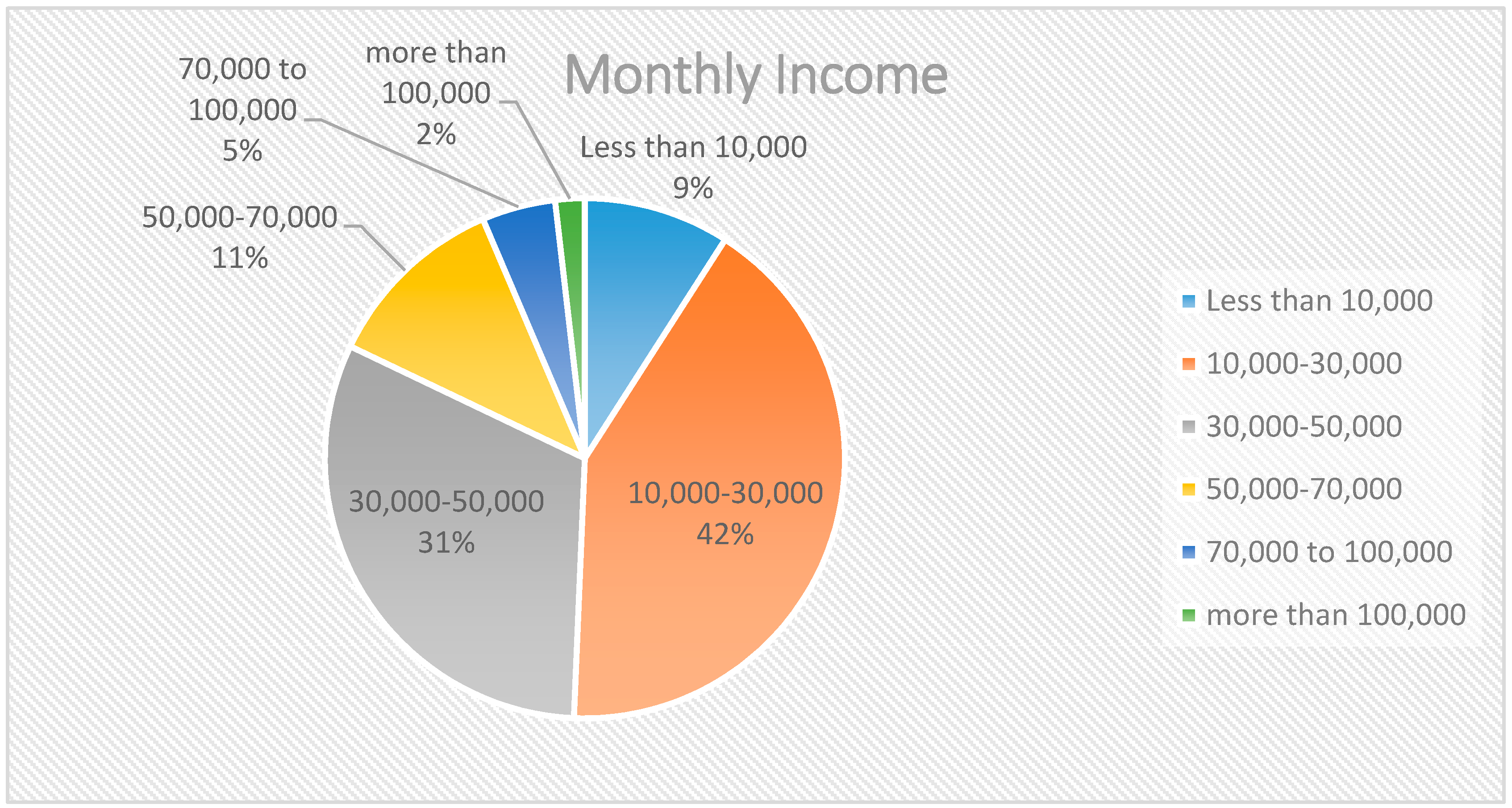
We also include several other household and location characteristics as exogenous variables affecting the demand for drinking water. These include household income, education, age, type of dwelling (e.g., single vs. double storey), and time to fetch water from different water sources (filtered and unfiltered). The sample data depicts that the average household income is PKR. 33,966. The sample statistics show that about 51 percent of the respondents belong to the lower or middle income group (See Pie chart in Figure 2). For instance, nine percent of the households have less than a PKR. 10,000 monthly income, whereas 42 percent earn between PKR. 10,000 to 30,000 per month, which is followed by an income group of PKR. 30,000–50,000 that comprises 31 percent of the entire sample. About 11% of the sample represents households having a monthly income of between PKR. 50,000 to 70,000. The income group earning PKR. 70,000–100,000 makes up 5% of the sample. Only 2% of the sample represents the high income group, who earn above PKR. 100,000.

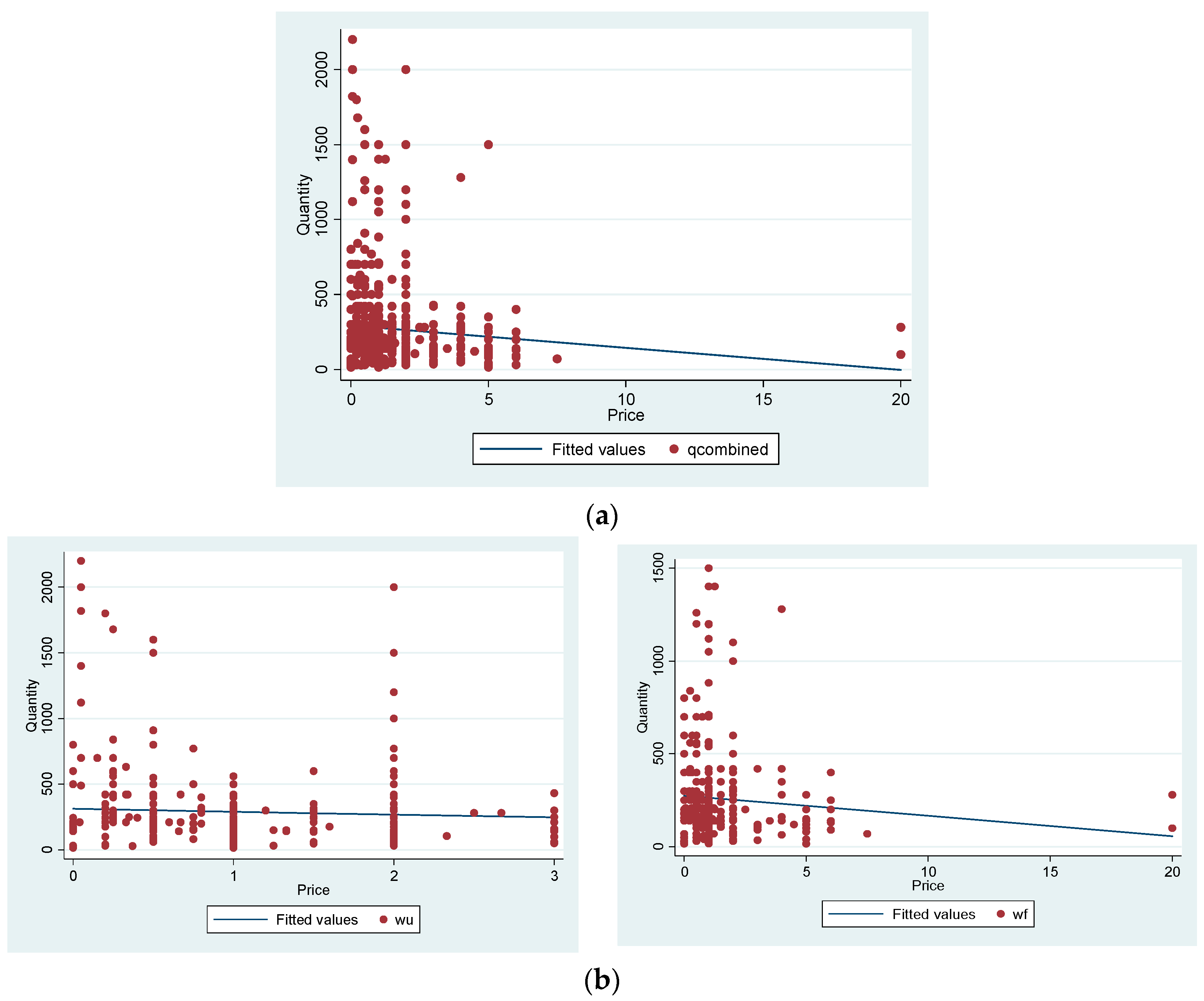
The sample’s statistics data show that households have on average received 10 years of schooling. The data further indicate that about 50% of sample participants completed high school, 25% attained a university education, and 10% of the respondents were found to be illiterate. The average age of families/persons living in the sample households is about 40 years, which varies from 18 years to 85 years. Since households obtain water from different filtered and unfiltered sources, they have to travel to fetch water from those sources. Our sample statistics show that on average it takes about 13 min to fetch water. We also note that about 28 percent of households have water leakages, and the average number of taps was recorded at seven per household. The data on household water expenditures show that expenditures on drinking water in summer are double that of household expenditures on drinking water in winter. Figure 2 presents a scatter plot of quantity of water against price per litre. We observe a negative relationship between quantities consumed and the price of water consumption (from all sources).

5. Empirical Results and Discussion

Considering the water price-setting mechanism by WASA in Faisalabad, prices may have been treated endogenously, and thus violate the orthogonality conditions, as price is correlated with the random terror term. As mentioned previously, in the presence of endogeneity, the OLS method will produce biased estimates of price elasticities. This issue can be resolved by estimating the demand equation in two steps. However, the two-step method is not efficient and produces incorrect standard errors. In this paper, we apply 2SLS and GMM methods to control the endogeneity issue and obtain corrected standard errors for water demand estimates. Further, to obtain robust standard errors, we also estimate all three demand functions using bootstrapping methods. Price was instrumented with the geographical indicator distance, media as an awareness indicator, and pipe leakages as a water quality indicator. In addition, we use water tank supply as an instrumental variable. We estimate three demand equations including combined (full sample), filtered, and unfiltered water consumption. We also conduct several tests for endogeneity and the validity of instruments in our estimated models. The statistics of these tests are presented in the estimates tables. The p-values of these tests indicate that the null hypothesis of exogeneity of the instruments is rejected strongly, as the F-test value is statistically significant at less than 1%. For instance, the F-Statistic value for the combined sample (i.e., 14.07 and respective p-value 0.000) indicates that we reject the null hypothesis that water price is exogenously determined. We also performed over-identification tests, and Woodridge test-statistics are presented in the estimates tables, which indicate that the instruments used in the estimation procedures are valid. The test statistics for the over-identifying restrictions are presented in the estimates tables. Further, we also apply the bootstrapping method to estimate different demand specifications, and our estimates are based on 10,000 replications.

Table 3. Two-stage least square estimation of residential water demand (Combined).

	Two Stage Least Square		Bootstrapping
Variables	Coefficients	Robust SE	Bootstrap SE	Z-value	p-value
Dependent Variable (log of combined quantity of water)
Log(Price)	−0.643 ***	0.109	0.115	−4.986	0.000
Log(Income)	0.067 *	0.038	0.042	2.451	0.014
Log(Age)	0.189 **	0.08	0.079	1.827	0.068
House Storeys	0.090 **	0.036	0.039	2.1	0.036
Number of Taps	0.012 **	0.005	0.005	2.132	0.033
Filter Dummy	0.01	0.051	0.049	0.012	0.991
Log (Education)	−0.099	0.075	0.073	−1.143	0.253
Log(Water Fetch Time)	−0.003	0.003	0.003	−1.305	0.192
Constant	3.787 ***	0.478	0.5	6.732	0.000
Sample Size	1100	---	---	---	---
Over-identification (${\chi }^2$)	9.516	---	---	---	0.147

Notes: * p < 0.10, ** p < 0.05, ***, p < 0.01. SE, standard error.

reports the results of the 2SLS estimates of residential water demand for a combined sample. The estimates of demand and their respective standard errors are presented in columns 2 and 3. The estimates show that the own price elasticity of demand is negative and significant at a one percent level of significance. Our use of four different towns in Faisalabad city through stratified sampling assured greater representativeness and augmented our confidence in the results. Furthermore, the error estimates presented, and the supplemental qualitative research conducted, as part of our larger research project gives us adequate confidence in this output’s reliability. All of the estimates are based on a log-log model to directly infer the price and income elasticities of water demand. The coefficient of the own price elasticity (−0.43) suggests that demand is inelastic, implying that a 1% increase in the price of water causes a 0.43% decline in the quantity demand of water. The bootstrap standard errors, Z-values, and p-values are provided in columns 4, 5, and 6, respectively. The GMM estimates are provided in

Table A3. Generalized method of moment estimation of residential water demand (combined).

	GMM		GMM Bootstrapping
Variables	Coefficients	Robust SE	Bootstrap SE	Z-value	p-value
Dependent Variable (log of combined quantity of water)
Log(Price)	−0.636 ***	0.111	0.111	−5.72	0.000
Log(Income)	0.066 *	0.04	0.040	1.65	0.006
Log(Age)	0.186 **	0.077	0.077	2.41	0.087
House Storeys	0.095 ***	0.037	0.038	2.53	0.024
Number of Taps	0.012 **	0.005	0.005	2.35	0.019
Filter Dummy	0.011	0.049	0.047	0.22	0.905
Log (Education)	−0.003	0.003	0.003	−0.95	0.210
Log(Water Fetch Time)	3.798 ***	0.484	0.467	8.14	0.105
Constant	14.458	---	---	---	---
Sample Size	1100	---	---	---	0.000
Over-identification (${\chi }^2$)	9.51	---	---	---	0.147

Note: * p < 0.10, ** p < 0.05, *** p < 0.01.

(in the Appendix A), which are similar to our 2SLS estimates. These results are comparable with the earlier studies reported in the existing literature [17,19,24,27,40,41,42]. The low magnitude elasticity indicates that households have a relatively low share of water spending in their total expenditures.

The estimate of income remains significantly positive (i.e., 0.07), implying that households with higher income consume more water. It implies that a one percent increase in income leads to a 0.07% increase in demand of water. The empirical results of the price and income elasticities of demand suggest that water consumption is not very responsive to price and income changes in Pakistan. These findings do not differ significantly from those of other developing countries. These elasticities are in line with the previous literature, such as Stevens et al. [43]; Hoffman et al. [44]; Gaudin [45]; Nauges & Strand [30]; and Schleich and Hillenbrand [46]. Under an inelastic response to price changes, pricing policies have limited scope in changing water consumption patterns.

The residential demand for water is also likely to vary depending upon house and household characteristics, such as house type and household size. Household size is an important factor, which determines water demand. In the literature, many studies, such as Rietveld et al. [38], Martinez-Espineira [26], Hoffman et al. [44], and Nauges & Strand [30], have analysed a household size’s impact on residential water demand. These studies found a positive impact of household size on residential water demand. House storey was used as a proxy measure for household size. A house with a double storey or more indicates that the number of residents in the house is higher, as compared to a single storey house. The results indicate that that residents with a larger household size consume more water.

We include household characteristics and other control variables to determine the impact of exogenous factors affecting the demand for water in the urban areas of Faisalabad. The results show that age is positively associated with the demand of water, which is significant at a 5% significance level. Time cost is an important factor in the literature, which determines water demand (see, for example [4,47]. The empirical estimates turn out to be negative and insignificant, which implies that respondents that are residing near filtered or unfiltered water sources consume more water. We also introduce a house storeys variable as a proxy of house (or household) size. The coefficient of house storeys is significantly positive at a 5% level of significance. Similarly, an increased number of taps lead to an increase in water consumption. Education level also negatively related with water consumption, but remains insignificant. Other dummy variables were introduced in the model to assess whether the use of different water sources significantly drives household water consumption or not. To this end, a dummy variable was introduced for households using filtered water (filtered = 1, 0 otherwise). The households using filtered water consume less water, as compared to those using unfiltered water. However, this impact is insignificant.

Our estimates for the subsamples are presented in

Table 4. Two-stage least square estimation of residential water demand (filtered water).

	Two Stage Least Square		Bootstrapping
Variables	Coefficients	Robust SE	Bootstrap SE	Z-value	p-value
Dependent Variable (log of quantity of filtered water)
Log(Price)	−0.428 *	0.221	0.231	−1.826	0.068
Log(Income)	0.123 **	0.058	0.055	2.121	0.034
Log(Age)	0.352 ***	0.101	0.101	3.315	0.001
House Storeys	0.068	0.049	0.058	1.153	0.249
Log(Water Fetch Time)	−0.002	0.003	0.003	−0.746	0.456
Constant	2.753 ***	0.745	0.711	3.601	0.000
Sample Size	519	---	---	---
Over-identification	3.486	---	---	---	0.626

Note: * p < 0.10, ** p < 0.05, *** p < 0.01.

and

Table 5. Two-stage least square rstimation of residential water demand (unfiltered water).

	Two Stage Least Square		Bootstrapping
Variables	Coefficients	Robust SE	Bootstrap SE	Z-value	p-value
Dependent Variable (log of quantity of unfiltered water)
Log(Price)	−0.714 ***	0.116	0.128	−5.583	0.000
Log(Income)	0.013	0.054	0.058	0.217	0.828
Log(Age)	−0.034	0.12	0.116	−0.280	0.780
House Storeys	0.097 *	0.051	0.055	1.887	0.059
Number of Taps	0.017 **	0.008	0.008	2.119	0.034
Pipe Connection	0.054	0.074	0.076	0.697	0.486
Log(Water Fetch Time)	−0.002	0.004	0.004	−0.601	0.548
Constant	5.074 ***	0.703	0.712	6.789	0.000
Sample Size	581	---	---	---
Over-identification	9.702	---	---	---	0.1378

Note: * p < 0.10, ** p < 0.05, *** p < 0.01.

, respectively. The 2SLS estimates of the filtered water sample (Table 4) show that price and income elasticities are statistically significant with expected signs. The bootstrap standard errors and the p-values of the estimates are also provided in column 4 to 6 in the table, whereas the GMM estimates are presented in

Table A4. Generalized method of moment estimation of residential water demand (filtered).

	GMM		GMM Bootstrapping
Variables	Coefficients	Robust SE	Bootstrap SE	Z-value	p-value
Dependent Variable (log of quantity of filtered water)
Log(Price)	−0.488 **	0.234	0.209	−2.4	0.022
Log(Income)	0.232 ***	0.058	0.055	2.42	0.015
Log(Age)	0.261 ***	0.109	0.098	3.58	0.000
House Storeys	0.100 *	0.056	0.054	1.43	0.157
Log(Water Fetch Time)	−0.003	0.003	0.003	−0.72	0.494
Constant	2.668 ***	0.787	0.706	3.75	0.000
Sample Size	519	---	---	---	---
Over-identification	6.026	---	---	---	0.3037

Note: * p < 0.10, ** p < 0.05, *** p < 0.01.

(in the Appendix A). The own price elasticity of demand for filtered water is noted to be −0.43, again indicating that the demand for filtered water is inelastic. The income elasticity of demand is found to be 0.12. The estimates of age are found to be significantly positive, indicating that people in old age consume more filtered water. This may be the result of awareness or health care consciousness. In other words, increasing age necessitates the demand for clean water for/by elders, who are willing to pay more as prevention against water borne diseases. On the other hand, the estimates’ results suggest a negative relationship with water collection time and filtered water consumption, but it remains insignificant. There is an opportunity cost to fetch water from a distant filter plant, which may be reason for households to reduce their consumption of filtered water, in addition to their income and affordability to buy bottled water.

In addition, a dummy variable was used for piped connections. The results show a positive relationship with water consumption. In other words, households with a WASA connection are likely to use more water, compared with those who do not have a piped water facility. Similarly, the results’ estimates of households using tank water remain significantly positive, meaning that a one percent increase in tank water use increases overall water consumption by 0.15 percent. The price and income elasticities conform with the findings in many developing economies [44,48,49,50,51].

Table 5 reports the results based on our sample for the consumption of unfiltered water by the households (See also the GMM estimates in

Table A5. Generalized method of moment estimation of residential water demand (unfiltered).

	GMM		GMM Bootstrapping
Variables	Coefficients	Robust SE	Bootstrap SE	Z-value	p-value
Dependent Variable (log of quantity of filtered water)
Log(Price)	−0.734 ***	0.116	0.121	−6.05	0.000
Log(Income)	0.005	0.057	0.059	0.09	0.932
Log(Age)	−0.003	0.119	0.114	−0.03	0.977
House Storeys	0.095 *	0.049	0.055	1.72	0.083
Number of Taps	0.022 ***	0.008	0.008	2.86	0.004
Pipe Connection	0.02	0.074	0.078	0.26	0.789
Log(Water Fetch Time)	−0.001	0.004	0.004	−0.33	0.729
Constant	5.017 ***	0.716	0.715	7.02	0.000
Sample Size	581	---	---	---
Over-Identification		---	---	---
Over-identification (${\chi }^2$)	9.702	---	---	---	0.138

Note: * p < 0.10, ** p < 0.05, *** p < 0.01.

in the Appendix A). The price elasticity of demand for unfiltered water remains at −0.714, which remains the highest as compared with the previously discussed results for the other categories (i.e., with the full sample and filtered water sample data). However, the income elasticity of the estimates is quite low at 0.013, compared with the estimates’ results for the combined and filtered water samples. We also included pipe connection as a dummy variable, and the results indicate that households with a piped connection are likely to use more water. However, these estimates are not statistically significant in the analysis, which is positive but still remains insignificant. It implies that households having piped water are inclined to consume more water. The survey data reveals that tank water is generally considered as an economical and relatively safe drinking water source. We note that households having more taps are inclined to consume more water, which may be due to the fact that a large number of family members use the water facility.

6. Conclusions

This study examined urban residential water use in Faisalabad to identify the factors which influence variability in household water demand. Econometric methods were used to estimate the price and income elasticities of water demand across different groups of consumers. The study used the survey data of 1100 households collected from urban residents of Faisalabad, which is one of the largest cities and industrial hubs in Pakistan. We used instrumental variable (IV) methods to address endogeneity issues, which otherwise could produce biased and inconsistent estimates. We apply 2SLS and GMM methods to estimate the demand elasticities and impact of other exogenous variables on household water consumption. To further obtain the corrected standard errors for meaningful policy analysis, we applied bootstrapping methods to estimate the water demand for different sources. Nevertheless, the demand remained price inelastic across all of the consumer groups. Specifically, the estimates of price elasticity for the combined sample are noted to be −0.641, while the estimates for filtered and unfiltered water vary from −0.43 to −0.471, respectively. These findings are similar to many developed and developing countries’ estimates, suggesting that water demand in Faisalabad is likely to respond less to an increase in prices. In other words, pricing policies may have limited scope in changing water consumption. The findings reflect that income elasticities vary across different groups (i.e., from 0.01 to 0.12). It implies that water consumption changes disproportionately with varying income levels. This divergence in water consumption seems to be due to differences in income levels and social status.

Other possible factors used to analyse the water consumption differences across groups include age, distance to water facility, education, and water connections. The results show that age is positively and significantly associated with the demand of filtered water. The impact of distance to a water source is negative, implying that households residing near water sources tend to consume more water. The policy implication of this finding could be focus on locational and supply-side factors of water. The governmental intervention to increase water supply points or the direct supply of clean water can substantially affect residential water demand.

The findings of the study also suggest that non-pricing tools should be explored, since the efficacy of pricing is constrained by numerous socioeconomic and governance factors. These tools could include creating water saving awareness through educational campaigns, informational tools, and encouraging the use of water efficient devices. Norms on the extraction of groundwater through household boring and the heavy subsidizing of aquifer water extraction limit price efficacy as well. Pricing signals that come from health awareness about the benefits of clean water must remain an essential part of public management in Pakistan. The household demand estimates inform various key messages for the water planning management of Faisalabad, WASA. These messages include the need for an appropriate pricing structure, and improving the water supply infrastructure in urban areas, which have been marginally noted in the Punjab government’s water and sanitation sector development plan up to 2024 [52].

Lastly, to achieve the goals of clean and sustainable water consumption, the local government and Water and Sanitation Authorities need to increase the coverage of drinking water facilities in priority low income areas that lag behind other dwellings. This calls for the need of appropriate policies for ensuring equity by removing disparities.

Ultimately, the essential need for water for all human systems will necessitate a rapid assessment of water demand and the consequent pricing mechanisms. Our study has attempted to show how a field-based survey can be implemented and analysed with a relatively low cost and time investment to inform policy decisions around water in a dense, developing urban context. Sustainable development goals around water and health will be key drivers in sustainable city planning and achieving smart growth in developing countries. There is no room for complacence in furthering our understanding of the water-development nexus. New demands for resources and technologies for modern infrastructure will also create new demands on water. This paper has contributed towards highlighting the opportunities and challenges of effective pricing mechanisms for water, and the ways of making a more cogent connection between urban analytics and environmental policy.

References

- Kenway, J.S.; Lant, P.A. How does energy efficiency effect urban water system? In Understanding Ad Managing Water in Transition; Grafton, Q., Daniell, K., Nauges, C., Rinaudo, J., Chan, N.W., Eds.; Springer: Berlin, Germany, 2015. [Google Scholar]
- Nauges, C.; Whittington, D. Estimation of water demand in developing countries: An overview. World Bank Res. Obs. 2010, 25, 263–294. [Google Scholar] [CrossRef]
- Rizaiza, O. Residential water usage: A case study of the major cities of the western region of Saudi Arabia. Water Res. Res. 1991, 27, 667–671. [Google Scholar] [CrossRef]
- Nauges, C.; Van Den Berg, C. Demand for piped and non-piped water supply services: Evidence from Southwest Sri Lanka. Environ. Res. Econ. 2009, 42, 535–549. [Google Scholar] [CrossRef]
- UNESCO. Water in the Post-2015 Development Agenda and Sustainable Development Goals, Discussion Paper, UNESCO International Hydrological Programme. Available online: http://unesdoc.unesco.org/images/0022/002281/228120e.pdf (accessed on 19 June 2014).
- OECD. Managing Water for All: An OECD Perspective on Pricing and Financing; Organization for Economic Co-Operation and Development: Paris, France, 2009; Available online: http://www.oecd.org/tad/sustainable-agriculture/44476961.pdf.2009 (accessed on 16 July 2017).
- Kugelman, M. Urbanization in Pakistan: Causes and Consequences, Norwegian Peacebuilding Resource: Centre. Available online: www.gsdrc.org (accessed on 10 March 2015).
- Akhtar, N.; Jamil, A.; Noureen, H.; Imran, M.; Iqbal, I.; Alam, A. Impact of Water Pollution on Human Health in Faisalabad City. Pak. J. Agric. Soc. Sci. 2005, 1, 43–44. [Google Scholar]
- Faisalabad Urban Structure Plan—2015. Available online: http://faisalabad.gov.pk/assets/uploads/Downloads/FPUSP%20Final%20Report.pdf (accessed on 20 March 2016).
- Pakistan Bureau of Statistics. Available online: http://www.pbs.gov.pk/sites/default/files//tables/District%20at%20a%20glance%20Faisalabad.pdf (accessed on 20 March 2016).
- Faisalabad City Government. Available online: http://www.faisalabad.gov.pk/Home/Towns (accessed on 21 March 2016).
- Water and Sanitation Authority of Faisalabad (WASA). Faisalabad Website. Available online: http://www.wasafaisalabad.gop.pk (accessed on 10 April 2017).
- Arubes, F.; Gracia-Valinas, M.A.; Martinez-Espeneira, R. Estimation of residential water demand: A state of the art review. J. Socioecon. 2003, 32, 81–102. [Google Scholar]
- Howe, C.W.; Linaweaver, F.P. The impact of price on residential water demand and its relation to system design and price structure. Water Res. Res. 1967, 3, 13–32. [Google Scholar] [CrossRef]
- Gibbs, K.C. Price variable in residential water demand models. Water Res. Res. 1978, 14, 15–18. [Google Scholar] [CrossRef]
- Danielson, L.E. An analysis of residential demand for water using micro time—Series data. Water Resour. Res. 1979, 15, 763–767. [Google Scholar] [CrossRef]
- Agthe, D.E.; Billings, R.B. Dynamic models of residential water demand. Water Res. Res. 1980, 16, 476–480. [Google Scholar] [CrossRef]
- Schefter, J.E.; David, E.L. Estimating residential water demand under multi-part tariffs using aggregate data. Land Econ. 1985, 61, 272–280. [Google Scholar] [CrossRef]
- Chicoine, D.L.; Ramamurthy, G. Evidence on the specification of price in the study of domestic water demand. Land Econ. 1986, 62, 26–32. [Google Scholar] [CrossRef]
- Nieswiadomy, M.L.; Molina, D.J. Comparing residential water demand estimates under decreasing and increasing block rates using household data. Land Econ. 1989, 65, 280–289. [Google Scholar] [CrossRef]
- Point, P. Partage de la ressource en eau et demande d'alimentation en eau potable. Revue Écon. 1993, 44, 849–862. [Google Scholar]
- Hansen, L.G. Water and energy price impacts on residential water demand in Copenhagen. Land Econ. 1996, 72, 66–79. [Google Scholar] [CrossRef]
- Agthe, D.E.; Billings, R.B. Water-price effect on residential and apartment low-flow fixtures. J. Water Res. Plan. Manag. 1996, 122, 20–23. [Google Scholar] [CrossRef]
- Renwick, M.E.; Archibald, S.O. Demand side management policies for residential water use: Who bears the conservation burden? Land Econ. 1998, 74, 343–359. [Google Scholar] [CrossRef]
- Höglund, L. Household demand for water in Sweden with implications of a potential tax on water use. Water Res. Res. 1999, 35, 3853–3863. [Google Scholar] [CrossRef]
- Martinez-Espineira, R. Estimating water demand under increasing-block tariffs using aggregate data and proportions of users per block. Environ. Res. Econ. 2003, 26, 5–23. [Google Scholar] [CrossRef]
- Nauges, C.; Thomas, A. Privately operated water utilities, municipal price negotiation, and estimation of residential water demand: The case of France. Land Econ. 2000, 76, 68–85. [Google Scholar] [CrossRef]
- Martínez-Espiñeira, R. Residential water demand in the Northwest of Spain. Environ. Res. Econ. 2002, 21, 161–187. [Google Scholar] [CrossRef]
- Strand, J.; Walker, I. Water markets and demand in Central American cities. Environ. Dev. Econ. 2005, 10, 313–335. [Google Scholar] [CrossRef]
- Nauges, C.; Strand, J. Estimation of non-tap water demand in Central American cities. Res. Energy Econ. 2007, 29, 165–182. [Google Scholar] [CrossRef]
- Basani, M.; Isham, J.; Reilly, B. The determinants of water connection and water consumption: Empirical evidence from a Cambodian household survey. World Dev. 2008, 36, 953–968. [Google Scholar] [CrossRef]
- Katzman, M. Income and price elasticities of demand for water in developing countries. Water Res. Bull. 1977, 13, 47–55. [Google Scholar] [CrossRef]
- Mu, K.; Whittington, D.; Briscoe, J. Modeling village water demand behavior: A discrete choice approach. Water Resour. Res. 1990, 26, 26–521. [Google Scholar] [CrossRef]
- McPhail, A.A. Why Don’t Households Connect to the Piped Water System? Observations from Tunis, Tunisia. Land Econ. 1994, 70, 189–196. [Google Scholar] [CrossRef]
- Persson, T.H. Household Choice of Drinking–Water Source in the Philippines. Asian Econ. J. 2002, 16, 303–316. [Google Scholar] [CrossRef]
- Wang, H.; Xie, J.; Li, H. Water Pricing with Household Surveys: A Study of Acceptability and Willingness to Pay in Chongqing, China. China Econ. Rev. 2010, 21, 136–149. [Google Scholar] [CrossRef]
- Crane, R. Water markets, market reform and the urban poor: Results from Jakarta. World Dev. 1994, 22, 71–83. [Google Scholar] [CrossRef]
- Rietveld, P.; Rouwendal, J.; Zwart, B. Block Rate Pricing of Water in Indonesia: An Analysis of Welfare Effects. Bull. Indones. Econ. Stud. 2000, 36, 73–92. [Google Scholar] [CrossRef] [Green Version]
- Van den Berg, C.; Nauges, C. The willingness to pay for access to piped water: A hedonic analysis of house prices in Southeast Sri Lanka. Lett. Spat. Res. Sci. 2012, 5, 151–166. [Google Scholar] [CrossRef]
- Thomas, J.F.; Syme, G.J. Estimating residential price elasticity of demand for water: A contingent valuation approach. Water Res. Res. 1988, 24, 1847–1857. [Google Scholar] [CrossRef]
- Gaudin, S.; Griffin, R.C.; Sickles, R.C. Demand specification for municipal water management: Evaluation of the Stone-Geary form. Land Econ. 2001, 77, 399–422. [Google Scholar] [CrossRef]
- Dharmaratna, D.; Harris, E. Estimating residential water demand using the stone-geary functional form: The case of Sri Lanka. Water Res. Manag. 2012, 26, 2283–2299. [Google Scholar] [CrossRef]
- Stevens, T.H.; Miller, J.; Willis, C. Effect of price structure on residential water demand. Water Res. Bull. 1992, 28, 681–685. [Google Scholar] [CrossRef]
- Hoffmann, M.; Worthington, A.; Higgs, H. Urban water demand with fixed volumetric charging in a large municipality: The case of Brisbane, Australia. Aust. J. Agric. Res. Econ. 2006, 50, 347–359. [Google Scholar] [CrossRef]
- Gaudin, S. Effect of price information on residential water demand. Appl. Econ. 2006, 38, 383–393. [Google Scholar] [CrossRef]
- Schleich, J.; Hillenbrand, T. Determinants of residential water demand in Germany. Ecol. Econ. 2009, 68, 1756–1769. [Google Scholar] [CrossRef]
- Briand, A.; Nauges, C.; Strand, J.; Travers, M. The impact of tap connection on water use: The case of household water consumption in Dakar, Senegal. Environ. Dev. Econ. 2010, 15, 107–126. [Google Scholar] [CrossRef]
- Martin, W.E.; Thomas, J.F. Policy relevance in studies of urban residential water demand. Water Res. Res. 1986, 22, 1735–1741. [Google Scholar] [CrossRef]
- Dandy, G.; Nguyen, T.; Davies, C. Estimating residential water demand in the presence of free allowances. Land Econ. 1997, 73, 125–139. [Google Scholar] [CrossRef]
- Martínez-Espineira, R. An estimation of residential water demand using co-integration and error correction techniques. J. Appl. Econ. 2007, 10, 161–184. [Google Scholar]
- De Maria André, D.; Carvalho, J.R. Spatial determinants of urban residential water demand in Fortaleza, Brazil. Water Res. Manag. 2014, 28, 2401–2414. [Google Scholar] [CrossRef]
- Government of Punjab. Drinking Water, Sanitation and Hygiene Development Plan 2014–2024. Available online: http://www.pndpunjab.gov.pk/system/files/Punjab%20WASH%20Sector%20Development%20Plan%202014-24.pdf (accessed on 14 July 2017).
Figure 1.
Water and Sanitation Authority (WASA) Water Supply Services Areas. Source: WASA Six-Year Business Plan (2014/15–2019/20).
Figure 2.
Relationship between Price and Quantity of Water. (a) Full sample (combined); (b) Filtered and unfiltered water.