New Potentiometric Wireless Chloride Sensors Provide High Resolution Information on Chemical Transport Processes in Streams


1
School of Environmental Systems Engineering, The University of Western Australia (M015), 35 Stirling Highway, Crawley WA 6009, Australia
2
Life and Veterinary Science, Murdoch University, 90 South Street, Murdoch, WA 6150, Australia
3
Department of Environmental Research and Innovation, Catchment and Eco-hydrology research group, Luxembourg Institute of Science and Technology, 41 rue du Brill, L-4422 Belvaux, Luxembourg
4
School of Electronics and Computer Science, University of Southampton, University Road, Southampton SO17 1BJ, UK
*
Author to whom correspondence should be addressed.
Water 2017, 9(7), 542; https://doi.org/10.3390/w9070542
Submission received: 26 May 2017
/
Revised: 11 July 2017
/
Accepted: 14 July 2017
/
Published: 19 July 2017
(This article belongs to the Special Issue New Developments in Methods for Hydrological Process Understanding)
Abstract
:Quantifying the travel times, pathways, and dispersion of solutes moving through stream environments is critical for understanding the biogeochemical cycling processes that control ecosystem functioning. Validation of stream solute transport and exchange process models requires data obtained from in-stream measurement of chemical concentration changes through time. This can be expensive and time consuming, leading to a need for cheap distributed sensor arrays that respond instantly and record chemical transport at points of interest on timescales of seconds. To meet this need we apply new, low-cost (in the order of a euro per sensor) potentiometric chloride sensors used in a distributed array to obtain data with high spatial and temporal resolution. The application here is to monitoring in-stream hydrodynamic transport and dispersive mixing of an injected chemical, in this case NaCl. We present data obtained from the distributed sensor array under baseflow conditions for stream reaches in Luxembourg and Western Australia. The reaches were selected to provide a range of increasingly complex in-channel flow patterns. Mid-channel sensor results are comparable to data obtained from more expensive electrical conductivity meters, but simultaneous acquisition of tracer data at several positions across the channel allows far greater spatial resolution of hydrodynamic mixing processes and identification of chemical ‘dead zones’ in the study reaches.
1. Introduction
There is ongoing interest in understanding and quantifying the travel times and dispersion of solutes moving through stream environments, including the hyporheic zone and/or in-channel dead zones, where retention affects biogeochemical cycling processes that are critical to stream ecosystem functioning [1,2]. Streambed morphology is known to affect various exchange processes [3], and thus influence the residence time of advected solutes.
Information on chemical transport processes in streams can be obtained from introduced tracers that are usually injected instantaneously or at constant rate [4] at an upstream location under constant flow conditions and measured at one or more downstream locations in the main channel [5]. The acquisition of such data can be expensive and time consuming, so many modelling studies of chemical transport in streams have tended to rely on relatively few well documented field case studies, such as Uvas Creek, California, USA [6,7], and studies in South America [8] and Europe [9]. A particularly broad study of available data synthesized results of 162 tracer injections performed in 87 streams, resulting in a pooled dataset of 633 breakthrough curves [10]. Remarkably, 94% of these breakthrough curves exhibited experimental truncation (cessation of sampling before tracer concentrations returned to background levels), which leads to difficulties in resolving the form of the storage residence time distribution. Furthermore the data are limited to individual mid-channel breakthrough curves and therefore provide no information on cross-channel variability of chemical transport.
This points to a need for improved sampling protocols and new measurement methods that can provide simultaneous automated recording of chemical concentrations at a variety of in-stream locations to more comprehensively evaluate residence time behavior [10].
Today, there is a pressing need for new ecohydrological measurement systems that can acquire data at high temporal and dense spatial scales at affordable costs [11,12] and in this paper we apply new potentiometric chloride sensors [13] to obtain critical information on how in-channel flow conditions affect the distribution of tracer concentrations across the channel. The advantage of our sensor system is that simultaneous measurements can be made in a distributed array to obtain data with dense spatial and high temporal resolution for monitoring chemical transport and mixing processes in the environment. The sensing element we describe is low cost due to batch production (less than one Euro per sensor) and there is a significant cost advantage in having multiple sensors per set of logging equipment. A single logging system as described costs about Euro 300 for 7 measuring points (Euro 42 per sensing point) using off the shelf microprocessor boards, plus the cost of one reference electrode (Euro 50) per logging system (Euro 7 per sensing point).
The illustrative application presented here is to monitor in-stream hydrodynamic transport and dispersive mixing of an injected chemical, in this case NaCl. In detail, we present a proof of concept for use of the potentiometric sensors in streams and compare mid-channel concentration vs. time curve data with information obtained from conventional electrical conductivity sensors. Further innovation of the paper relates to recording and describing two dimensional (cross channel) tracer concentration curves across five shallow stream reaches with various bed morphologies and increasing levels of channel complexity in Luxembourg and Western Australia.
We show that the sensor system offers a hitherto unprecedented opportunity to record the full cross-channel spatial pattern of an injected tracer distribution. Such data is invaluable for enhanced validation of chemical mixing models and parameterization of exchange processes with the hyporheic zone.
2. Materials and Methods
2.1. Sensor Description
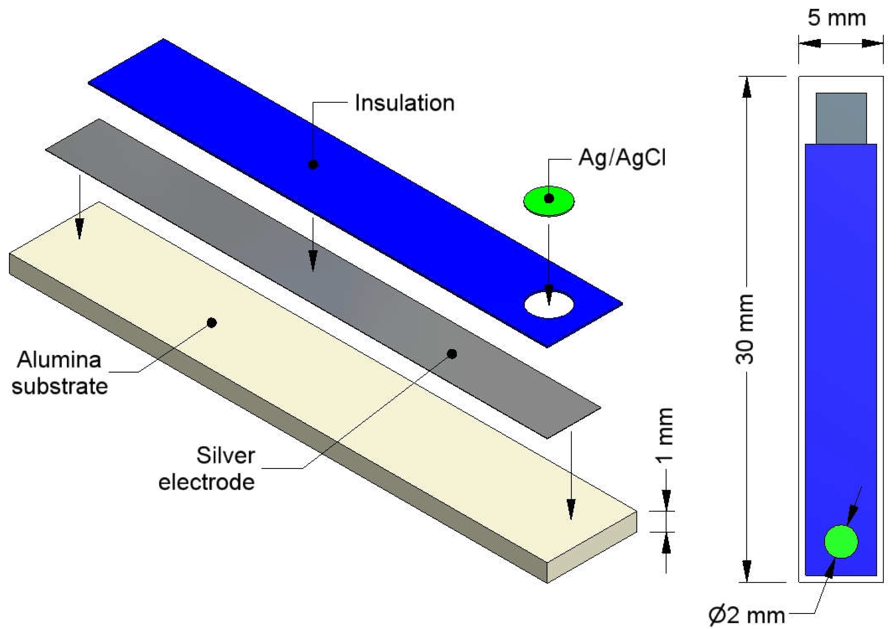
The chloride sensors used in this study have been described in detail [14] and initial proof of concept applications in controlled environments reported [13]. They are potentiometric sensors that generate an electrical potential proportional to the local chloride concentration. Low cost sensor manufacture is achieved using an industry-standard screen printing process that prints a silver layer onto an alumina substrate. A patterned insulating layer is then printed over the majority of the silver layer, which defines the active layer of the electrode structure and leaves a short end free for a soldered electrical connection. The exposed silver layer is electrochemically chloridized, producing a silver chloride layer over the silver electrode. The resulting electrical response generated by the structure is theoretically governed by the Nernst equation, yielding a sensitivity of −59.2 mV per decade change in chloride concentration (pCl) at 298 K temperature as given by
where E is the measured electrical potential (V), E0 is the offset potential (V), and CCL is the chloride ion concentration (M).
E = E0 − 0.0592log(CCL),
Sensor calibrations in standard solutions yielded a near-Nernstian response of −49.8 (±1.7) mV per decade change in chloride concentration and was consistent across sensors [14].
In order to complete the electrical circuit, measurements are made with respect to the reference potential of a commercial Ag/AgCl reference electrode (VWR GelPlas, 3.5 M KCl).
2.2. Sensor Electronics
The custom built system architecture for the sensor logging system has been previously described in detail [13]. However, it is useful to summarize this system. Figure 1a shows a picture of the system and Figure 1b the overall system diagram.
The electronics consists of an analog data conditioning board, which is connected to a digital processing board. The analog board is connected to the sensors and allows individual sensors to be connected sequentially to an amplifier. The output from the amplifier is then digitized by an analog to digital converter (ADC) under the control of the central microcontroller (MCU). This is then responsible for either transmitting the data at 2.4 GHz using the IEEE802.15.4 standard, sending it serially via USB to a connected computer, or storing it on the memory card. Currently the digital board is based on a Waspmote Open Source sensor node using an Atmel microcontroller [15]. This platform has both radio and SD card interfaces. In this study the data were digitized from the analog board using the on-board ADC with 10-bit resolution and then scaled, time stamped, and stored on the SD card for later retrieval.
The analog board allows for up to seven sensors to be connected and measured against a single reference electrode, which gives a fixed potential against which the sensors could be measured. The sensors can be distributed up to the length of their cable, and typically this would be between 1 m and 10 m long. Thus, it is possible to measure up to seven distributed points, or seven co-located points with one logger system. In experiments where more measurement positions are needed, it is possible to run multiple loggers, but this requires the logger’s real-time clocks (RTC) to be synchronized. With this system this is done by running a separate program to extract the time from a GPS module that can optionally be installed into each logger and using this to set the real time clock to an accuracy of 0.16 s per day. The GPS module also allows the position of the logger to be recorded in applications where loggers are widely spaced. The system also allows for changing the measuring interval wirelessly for flexible changing of application. Data can be wirelessly transmitted to a nearby collection/control point (usually a laptop PC) or can be stored locally on an SD memory card for later download. For this experiment, the requisite measurement time intervals were pre-programmed and readings were made sequentially from individual sensors through the analog multiplexer and stored locally for later extraction. For this stream sampling experiment, we used an 8 s measurement cycle. On each measurement cycle the system selects a sensor, allows the reading to settle for 30 milliseconds, taking 10 measurements for each sensor, and averages them. This is repeated for each sensor. These data are then written to the memory card and the system then reverts to a low-power sleep state until woken by an internal alarm at the next programmed measurement cycle.
The electronics were housed in a water proof box as shown in Figure 1a, with sensor cables grommeted through the casing. In this study, we tested sensors that were embedded in custom designed waterproof sleeves to protect the solder point from exposure, while leaving the sensor tip protruding. A schematic of the sensor construction and dimensions used in this study is shown in Figure 2.
2.3. Cross-Channel Distribution of Tracer Peak Arrival and Tailing Behavior
The cross-channel distribution of tracer peak arrival time indicates the effect of channel characteristics on flowlines from the injection point to the sensor locations. ‘Tailing’ [16] refers to asymmetrical tracer concentration curves arising from processes that alter the travel time distribution in the channel. For a non-reactive tracer this generally involves pressure driven exchanges with the hyporheic zone. Under steady streamflow conditions the degree of exchange can depend on factors such as bedslope irregularities and form, channel curvature, and permeability of bed and bank materials [17,18,19]. The degree of asymmetry can be assessed statistically by measuring skewness of the concentration curve [20].
For univariate data Y1, Y2…., YN, the Fischer-Pearson formula for skewness, is:
where is the mean, s is the standard deviation, and N is the number of data points.
Equation (2) was applied to all measured tracer curves obtained using the potentiometric sensors distributed across the channel and to curves from Electrical Conductivity (EC) sensors located at mid-channel.
3. Field Sites and Experimental Setup
We tested the sensor system on three small streams in the Attert river basin [21] in Luxembourg and at two locations along a stream in the Perth hills, Western Australia with different reach conditions and streambed morphologies. All three streams in Luxembourg (Rennbach, Weierbach, and Koulbich) have fixed gauging stations within 50 m of the experimental reaches, so independent discharge data were available for every tracer test. Neerigen Brook in the Perth Hills is no longer gauged so discharge estimates were obtained using the salt dilution method [22]. In Luxembourg the measurements were made under low summer flow conditions and in the Perth hills measurements were made in summer under recession flow conditions, four days after an intense storm exceeding 50 mm in a day had re-initiated stream flow in the previously dry channel.
In order of complexity, the channel sections can be described briefly as follows:
Reach 1: Neerigen Brook, Western Australia. Straight, artificially channelized riffle reach over Precambrian crystalline bed materials.
Reach 2: Neerigen Brook, Western Australia. Natural riffle-pool sequence with two approximately 30 degree bends along the study reach.
Reach 3: Weierbach, Luxembourg. Braided riffle-pool sequence through exposed schist bed material. Numerous small shallow pools along the braids.
Reach 4: Koulbich, Luxembourg. Artificially straightened riffle run leading to an eroded near bank pocket (right bank looking upstream). The pocket did not exhibit a backwater flow, but altered the flow pattern across the channel at the downstream exit.
Reach 5: Rennbach, Luxembourg. Natural riffle-shallow pool sequence that is relatively straight with exposed schist bed material in some of the riffles at the time of the tracer experiments. The measured cross-section partly extended across a confluence with the Koulbich in order to test the sensor response to channel mixing at this location. The site is within the confluence mixing location reported in a related study [23].
Upstream injection locations for sodium chloride were selected to optimize the opportunity for rapid complete mixing. At all locations, it was possible to locate a ‘throat’ where the channel narrowed, allowing the tracer to be introduced uniformly across the entire channel cross-section. At each location we also installed mid-channel electrical conductivity sensors (WTW Multi 3420 equipped with a TetraCon 925 probe, providing a conductivity resolution of 0.1 µS/cm from 0 µS/cm to 199 µS/cm and 1 µS/cm from 200 µS/cm to 1999 µS/cm), which were read manually at 5 s intervals for each tracer experiment. These sensors were calibrated to convert EC to NaCl, allowing results to be reported as Cl concentration for comparison with the chloride sensor data. All potentiometric sensors were calibrated individually using background water from each study reach. All results are then presented as C-Co, where Co is the background chloride concentration (g/L). We used an array of six sensors across transects at the first three sites and seven sensors across the latter two sites.
A summary of the main features of each experimental reach is given in Table 1.
4. Results
For each instrumented reach we present an annotated photograph of the reach, followed by tracer concentration curves for the first trace and tabulated data summarizing skewness (Equation (2)) and time to tracer peak for all traces performed at each location. Photographs have arrows indicating flow direction. The white circular marker in each photograph is used to indicate the right bank (looking upstream), which is the zero point on each transect. Measured channel widths are given in Table 1.
4.1. Neerigen Brook Reach 1
The instrumented cross-section is shown in Figure 3. The 25 m straightened section upstream from the transect has steep banks with some invasive grasses reaching the waterline along the channel banks.
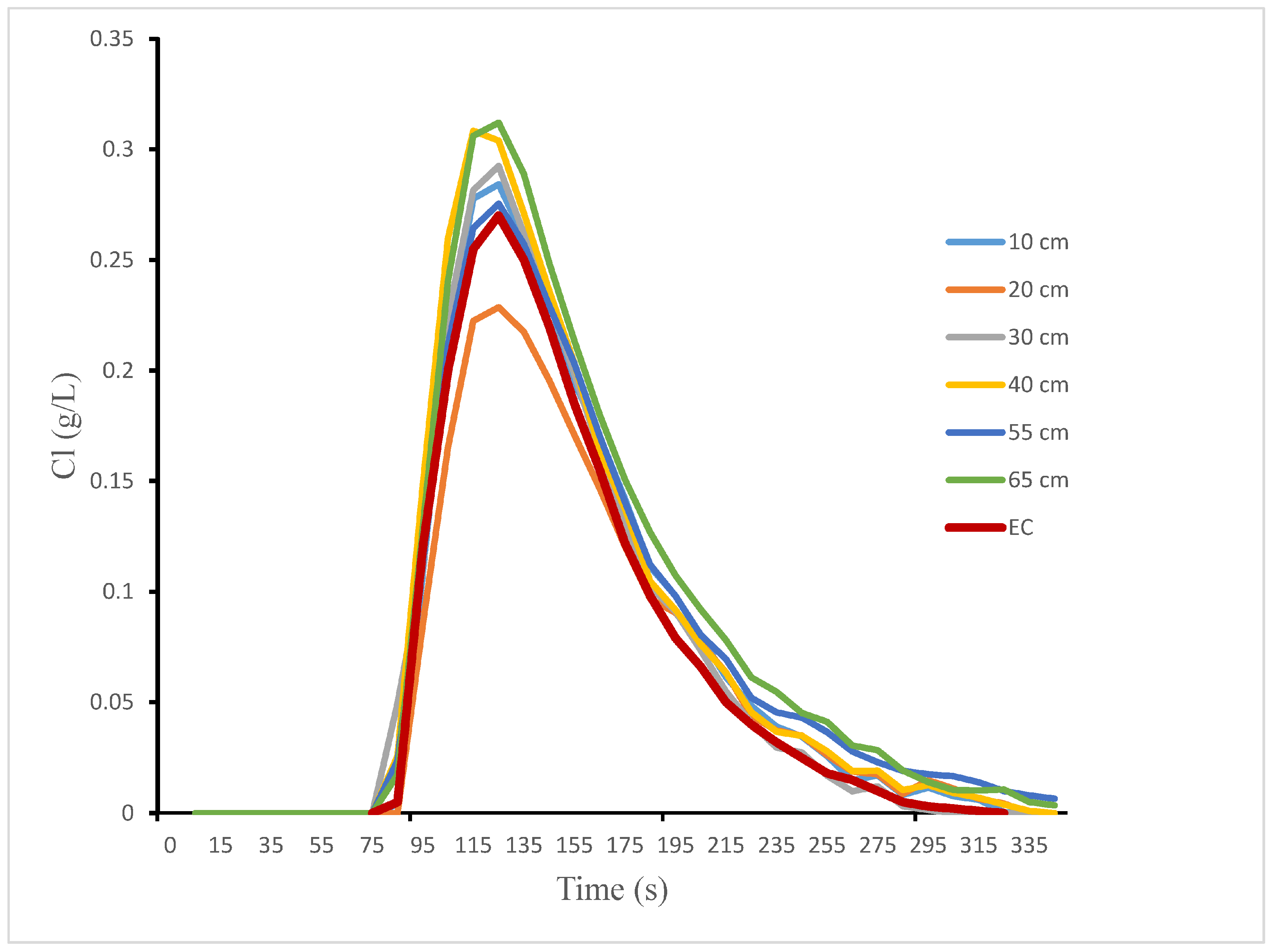
The cross-channel concentration curves for Neerigen Brook Reach 1 are shown in Figure 4. The calibrated mid-channel EC curve is shown for comparison with the data from the chloride sensors. Typically, all mid-channel calibrated EC curves were similar to mid-channel chloride sensor data.
For this straight section the cross-channel tracer curves have similar shapes, with tailing evident at all locations across the transect. The concentration peaks are similar, except at the 20 cm location where the peak concentration is lower.
Table 2 gives the results for skewness and time to peak. At all positions on the cross-section we found positive skew for all tracer runs. The EC probe was located about 35 cm across the channel and returned values of skew that were similar to those obtained from the chloride probes at 30 cm to 40 cm across the channel.
There is no obvious pattern to skew across the channel, indicating that bankside vegetation had little effect on tracer curve asymmetry. Similarly, peak arrival times were also unaffected, suggesting a minimal influence of vegetation induced drag along the banks.
4.2. Neerigen Brook Reach 2
The instrumented cross section is shown in Figure 5. Visibly the bed material ranged from gravel to cobbles and small rocks. Some pools contained a shallow layer of finer sand and silt sediments over the weathered crystalline bed. The section is about 2 km downstream from reach 1 and is wider and shallower. Discharge is similar to reach 1 but the flow rate had reduced to about 50% of reach 1 (Table 1).
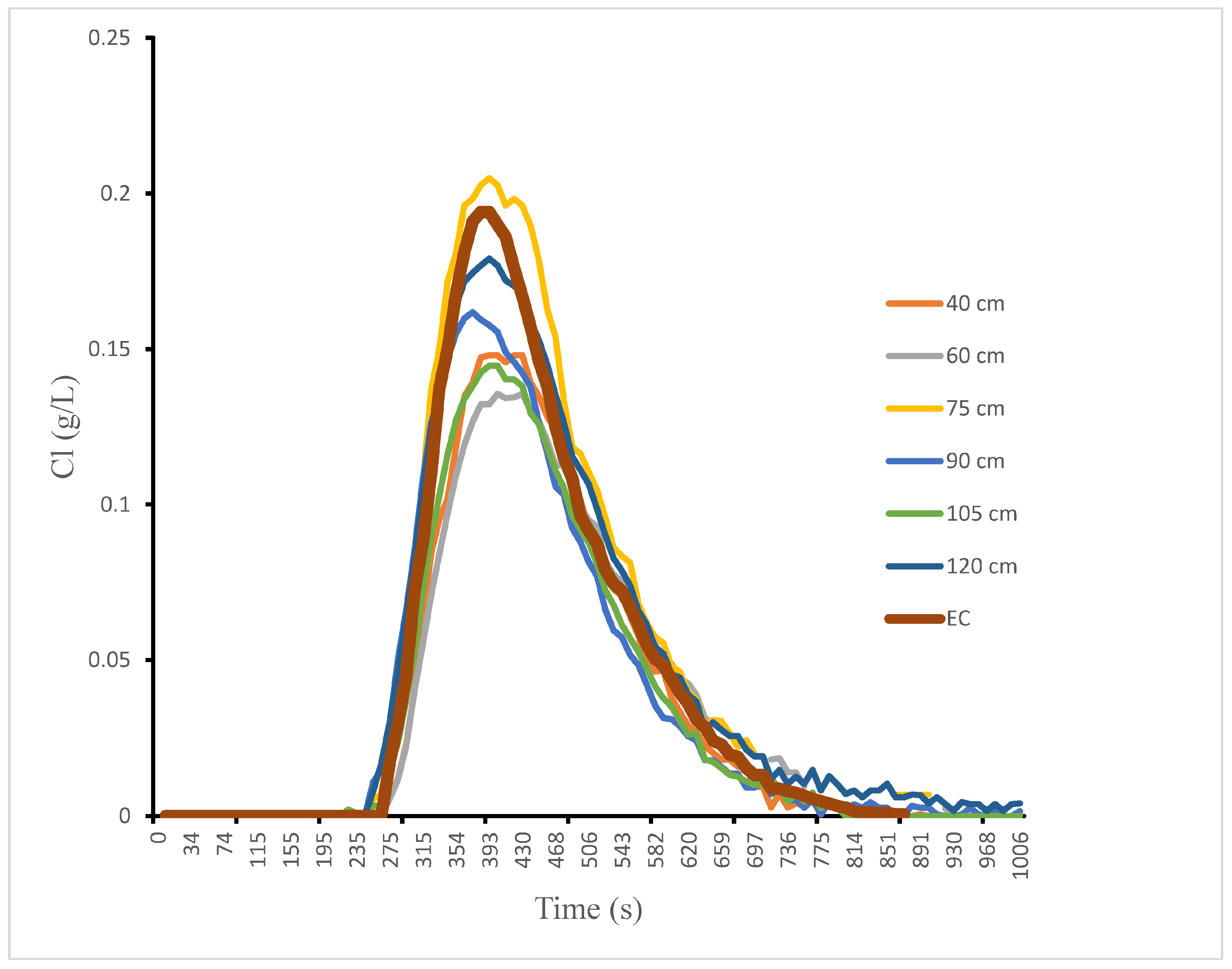
Concentration peaks given in Figure 6 are highest near mid-channel (75 cm), which is close to the position of the EC probe (installed at 70 cm). Low concentration peaks are visible at 40 cm and 60 cm. The cross-channel concentration curves in Figure 6 all exhibit tailing, with values of skew similar to Reach 1 (Table 3).
Across all runs and transect locations the range of skew is 0.85 to 1.08, with 78% of the values between 0.9 and 1.1.
Values of skew for the EC probe runs are similar to values returned from the mid-channel Cl probes at 60 cm to 75 cm. Times to peak vary between runs but there is evidence of lower times to peak at 90 cm and 75 cm. These are the only locations returning times to peak of less than 390 s.
4.3. Weierbach
The Weierbach channel with exposed rocks is shown in Figure 7a. To clearly identify the position of the sensors on the cross-section in relation to exposed rocks, a schematic is shown in Figure 7b.
Tracer data from the Weierbach are shown in Figure 8. Because of the very low discharge we reduced the tracer mass to 50 g NaCl for these traces. The right bank (looking upstream) from 0 cm to 15 cm across the measured transect was obstructed by rocks, followed by a deeper section (<1 cm) from 15 cm to 40 cm. From 40 cm to 110 cm the flow deepened to a maximum of 6 cm at 70 cm from the right bank. From this point to the left bank at 1.6 m the flow became very shallow again (<0.6 cm depth) with exposed rocks visible over 40% of the cross section.
The EC sensor was located at 75 cm and closely overlays the Cl sensor probe data at 70 cm and 85 cm.
The braided nature of the channel due to exposed schist resulted in a variety of possible flowpaths from the injection point to the sensors and this is reflected in the range of observed tracer shapes in Figure 8 and arrival times reported in Table 4. Peak arrival times varied from 217 s to 267 s and skewness varied from 0.84 to 1.86 across all runs and locations.
4.4. Koulbich
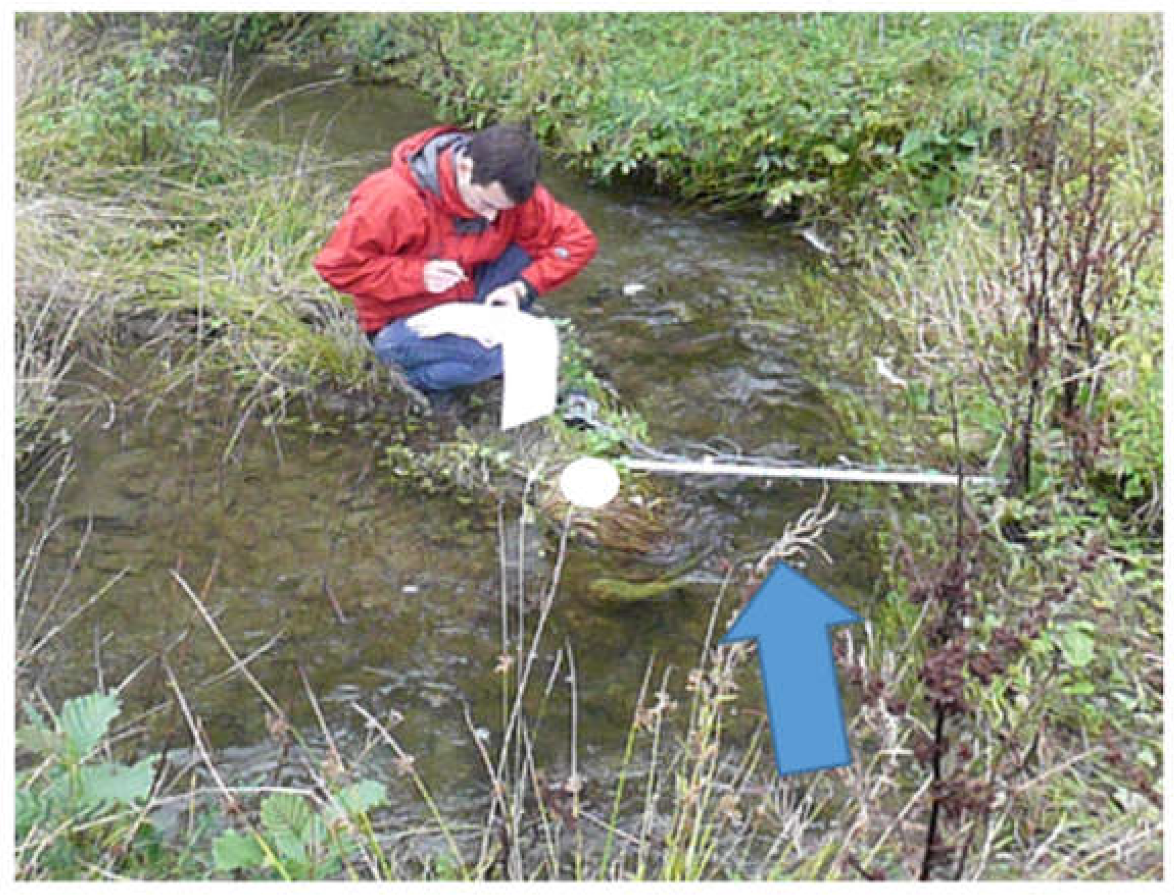
Figure 9 shows the undercut and scoured bank ‘pocket’ immediately upstream from the monitored cross-section on the Koulbich. Upstream from the flow arrow the reach is an artificially straightened riffle section through a meadow.
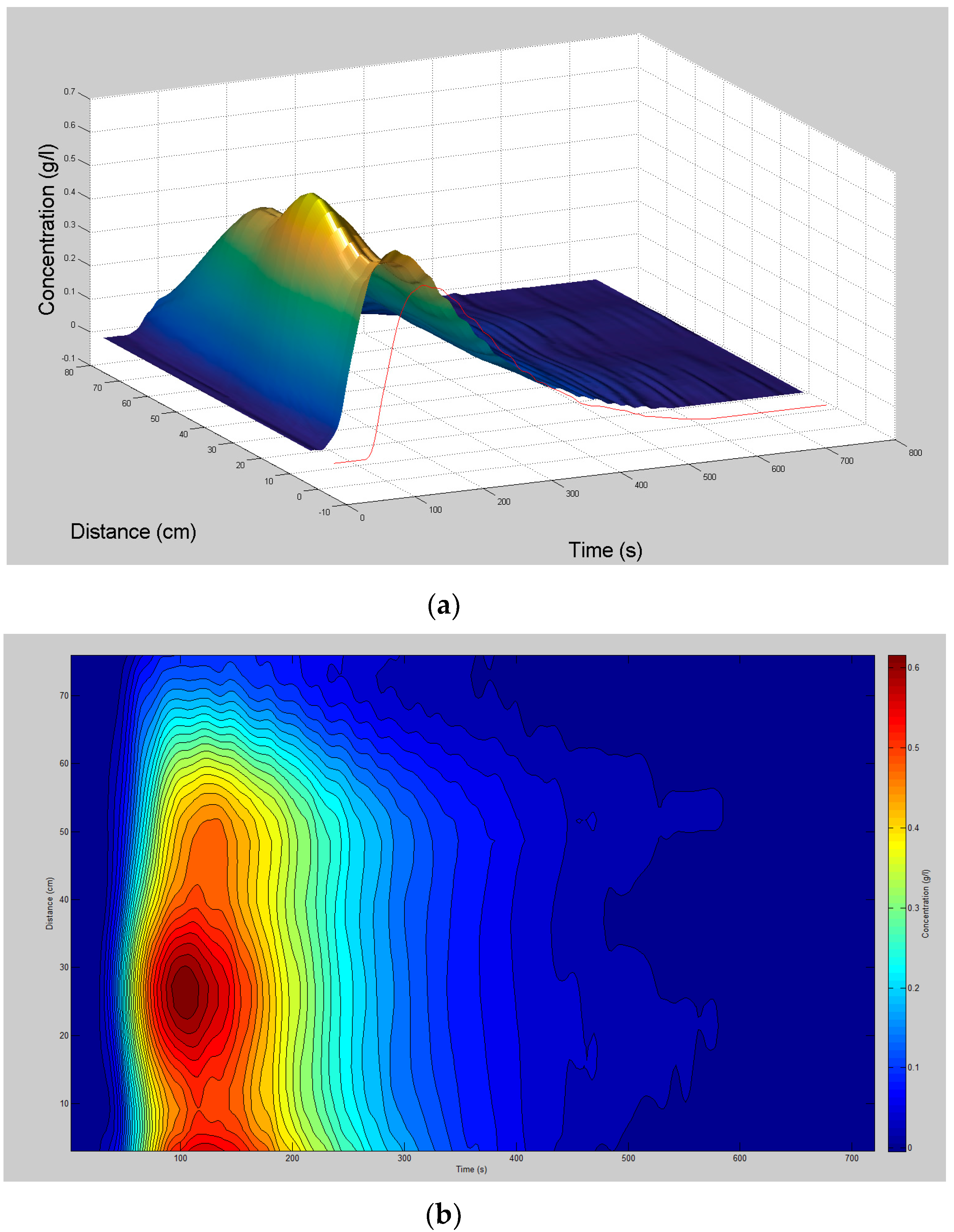
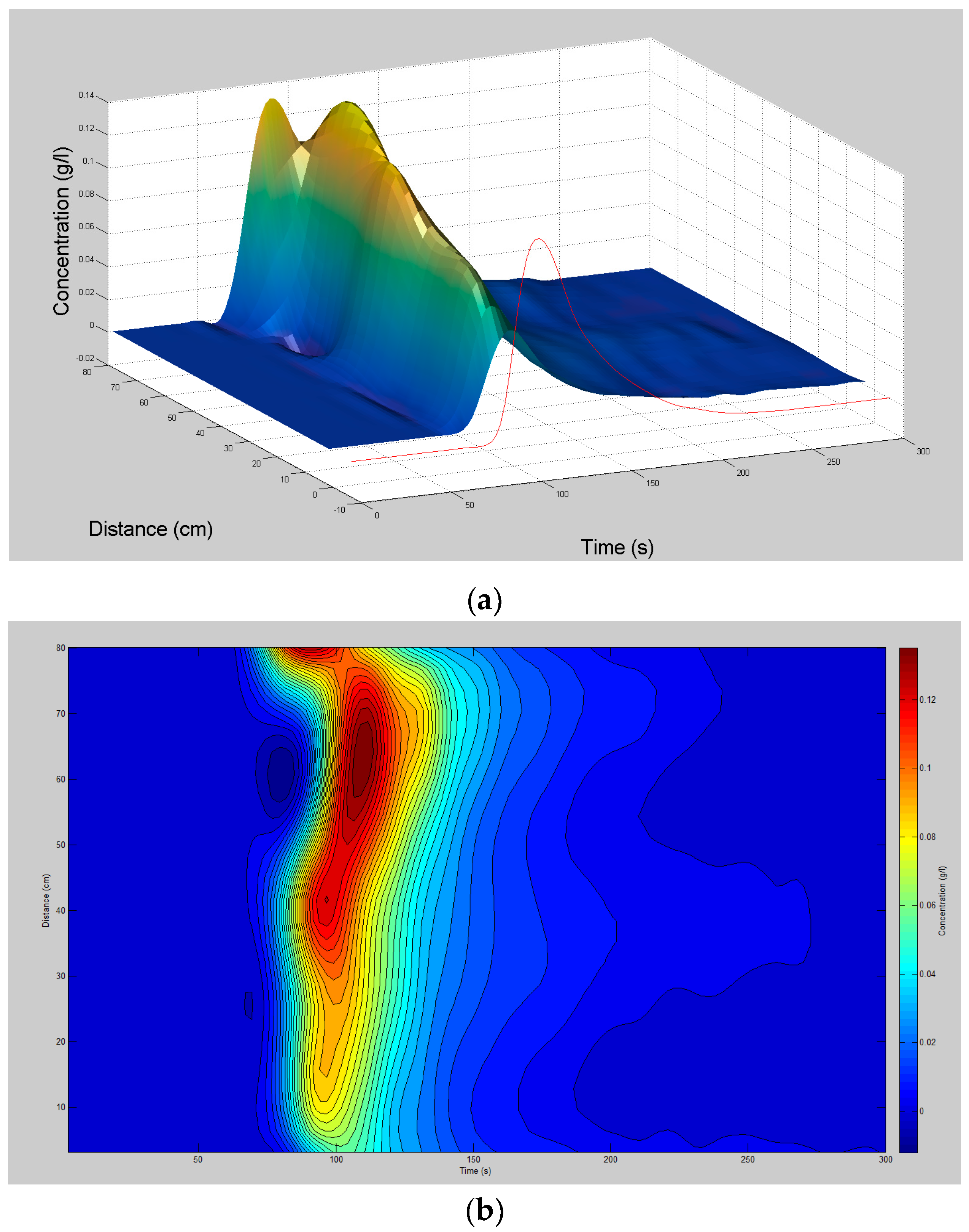
Tracer data (Figure 10a,b) reveal the influence of this pocket on tracer dilution, with highest peak concentrations recorded in sensors located to the left of the center line (looking upstream in Figure 9), in flow lines least influenced by the right bank scoured area. The scoured area did not however, influence peak arrival time at sensors to the left of the center line (Table 5). The tracer curve from the EC probe was again similar to the surrounding mid-channel probes at 40 cm and 55 cm (Figure 10a).
Values of skew ranged from 0.88 to 1.87 (Table 5), with considerable cross-transect and inter-run variation. The rank order of skewness across the transect was particularly unstable between runs. For example, the sensor at 24 cm returned the highest skew on run 2 and the lowest skew on run 3.
4.5. Rennbach-Koulbich Confluence
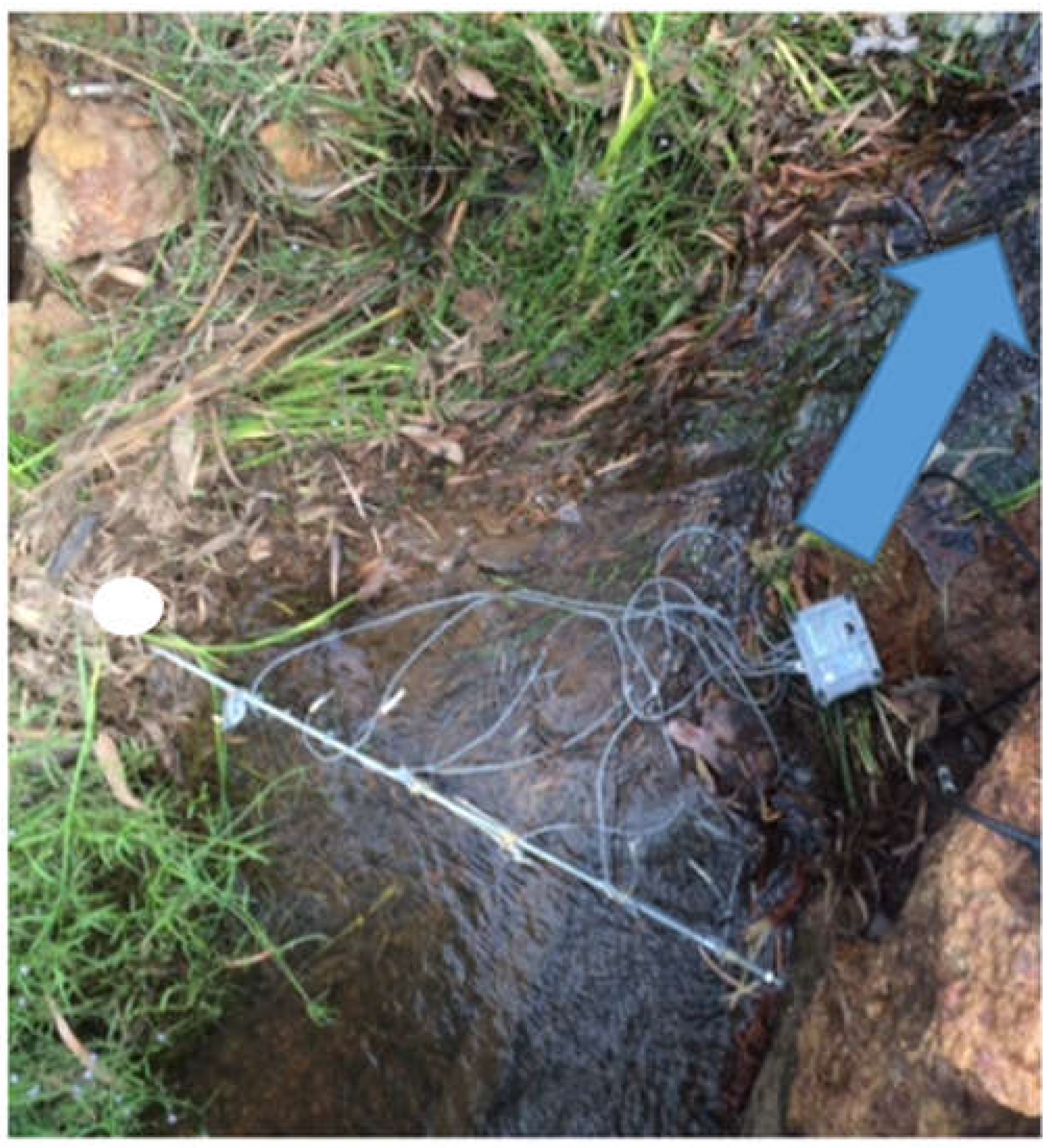
Figure 11 shows the position of the transect at the confluence of the Rennbach and Koulbich.
The effect of confluence mixing between the Rennbach and Koulbich is evident in Figure 12a,b with concentration peaks declining across the confluence mixing zone as the Koulbich flow influences dilution. However, tracer peak times across the transect were unaffected by confluence mixing (Table 6). All values of skew are less than 0.6, with 30% less than 0.26. Again, there is locational instability in the magnitude of skew between runs. All locations return at least one value of skew less than 0.26 and one value greater than 0.5 (Table 6).
5. Discussion
This study deployed new potentiometric sensors for in situ measurement of stream tracer breakthrough curves. Multiplexing via Waspmote loggers allowed for up to seven sensors to be simultaneously recorded on an individual logger. Using this approach, we were able to gain insight into cross-channel patterns of mixing and holdback at transects located downstream from a tracer injection point. A particular power of the setup is that many measurements can be made in a relatively short time. For example, using only four loggers we could obtain 84 tracer breakthrough curves from three runs and within a day it would be quite easy to generate the number of breakthrough curves pooled from decades of literature in [10]. The new sensor methodology thus completely addresses the call for more comprehensive evaluation of residence time behavior from simultaneous measurements at a variety of in-stream locations [10].
Results showed that at all sites the potentiometric sensors closest to the EC sensor location recorded tracer concentration time curves that closely followed the calibrated EC sensor, with similar values of skew. Both the potentiometric and EC sensors recorded a sharp concentration rising limb and more gradual falling limb at all locations, leading to positive values of skew throughout.
Interestingly, the artificially straightened channel section at Neerigen Brook Site 1 gave similar values of skew to the more natural riffle-pool section at Neerigen Brook Site 2. However, the large area of exposed bed and consequent ‘braided’ flow in the Weierbach led to more enhanced tailing and increased values of skew compared to the Neerigen Brook reaches.
The Koulbich also returned high values of skew, whereas the Rennbach-Koulbich mixing zone had the lowest values of skew. The latter result reflects a dominance of relatively symmetrical tracer transport along the Rennbach from the injection point, prior to mixing with the Koulbich at more distant sensors on the measured transect. This resulted in tracer concentration dilution with distance from the near bank, but did not affect tracer arrival time or skew.
Cross-channel patterns of tracer transport are clearly visible from the results. There are points across the channel, particularly for the last three sites, that differ substantially from the average mid-channel value. At each sensor these concentration curve patterns appear to be stable across all repeated tracer runs, although statistically, the absolute value of skewness can vary between runs.
The advantage of deploying sensor arrays is that cross-channel mixing behavior can be directly observed. By recording many measurements rapidly this new ecohydrological sensor array opens up possibilities for better parameterization of biogeochemical mixing processes that have generally relied on a single measure of holdback at mid-channel. The sensor array can of course be extended to multiple transects in order to follow the evolution of a chemical pulse downstream. The system can easily be extended to deeper and wider channels by using multiple time-synchronized loggers, thus opening up the possibility to obtain three-dimensional tracer distributions for enhanced validation of hydrodynamic mixing and exchange models.
6. Conclusions
We have shown for the first time in a field deployment that the calibrated potentiometric sensors record similar tracer curves to calibrated EC probes when installed at adjacent locations. The advantage of deploying potentiometric sensor arrays is that many more measurements can be taken at a fraction of the cost associated with the use of multiple EC probes. This opens up the opportunity to record tracer curves simultaneously at many locations in order to develop an enhanced three-dimensional understanding of mixing and exchange processes in streams. Such information gives the opportunity for enhanced calibration of three-dimensional in-stream transport models.
In this paper, we presented some examples of the type of information on hydrodynamic and exchange processes that can be extracted from installing probes in cross-channel arrays. We showed that this information can provide insight into how more complex morphological features may influence both the travel time and the exchange processes controlling the magnitude of holdback along stream flowpaths. We also identified situations where under steady-state flow conditions the skew can vary between successive tracer runs, leading to a need for correct identification of average holdback parameters in hydrodynamic mixing models.
Acknowledgments
This project has been supported by the Luxembourg National Research Fund FNR MOBILITY/16/11256906-SOLACE.
Author Contributions
Keith Smettem, Julian Klaus, Nick Harris, and Laurent Pfister contributed to the conception and design of the study; Nick Harris designed and programmed all logging protocols; Keith Smettem and Julian Klaus performed the experiments and analyzed the data; Keith Smettem, Julian Klaus, Nick Harris, and Laurent Pfister contributed to preparation of the manuscript.
Conflicts of Interest
The authors declare no conflict of interest.
References
- Argerich, A.; Haggerty, R.; Martí, E.; Sabater, F.; Zarnetske, J. Quantification of metabolically active transient storage (MATS) in two reaches with contrasting transient storage and ecosystem respiration. J. Geophys. Res. 2011, 116, G03034. [Google Scholar] [CrossRef]
- Gooseff, M.N.; Briggs, M.A.; Bencala, K.E.; McGlynn, B.L.; Scott, D.T. Do transient storage parameters directly scale in longer, combined stream reaches? Reach length dependence of transient storage interpretations. J. Hydrol. 2013, 483, 16–25. [Google Scholar] [CrossRef]
- Ward, A.S.; Schmadel, N.M.; Wondzell, S.M.; Harman, C.; Gooseff, M.N.; Singha, K. Hydrogeomorphic controls on hyporheic and riparian transport in two headwater mountain streams during base flow recession. Water Resour. Res. 2016, 52, 1479–1497. [Google Scholar] [CrossRef]
- Payn, R.A.; Gooseff, M.N.; McGlynn, B.L.; Bencala, K.E.; Wondzell, S.M. Channel water balance and exchange with subsurface flow along a mountain headwater stream in Montana, United States. Water Resour. Res. 2009, 45, W11427. [Google Scholar] [CrossRef]
- Harvey, J.W.; Wagner, B.J. Quantifying Hydrologic Interactions between Streams and Their Subsurface Hyporheic Zones, in Streams and Groundwaters; Jones, J.B., Mulholland, P.J., Eds.; Academic: San Diego, CA, USA, 2000; pp. 3–44. [Google Scholar] [CrossRef]
- Zand, S.M.; Kennedy, V.C.; Zellweger, G.W.; Avanzino, R.J. Solute transport and modelling of water quality in a small stream. J. Res. U.S. Geol. Surv. 1976, 4, 233–240. [Google Scholar]
- Avanzino, R.J.; Zellweger, G.W.; Kennedy, V.C.; Zand, S.M.; Bencala, K.E. Results of a Solute Transport Experiment at Uvas Creek, September, 1972; Open-File, Report 84-236; US Geological Survey: Menlo Park, CA, USA, 1984.
- Brevis, W.; Debels, P.; Vargas, J.; Link, O. Comparison of Methods for Estimating the Longitudinal Dispersion Coefficient of the Chillán River, Chile; Comparación de Métodos para estimar el coeficiente de dispersión longitudinal en el Río Chillán, Chile; Anales de XV Congreso Chileno de Ingenieriá Hidráulica, Sociedad Chilena de Ingenieriá Hidráulica: Concepción, Chile, 2001; pp. 155–164. (In Spanish) [Google Scholar]
- De Smedt, F.; Brevis, W.; Debels, P. Analytical solution for solute transport resulting from instantaneous injection instreams with transient storage. J. Hydrol. 2005, 315, 25–39. [Google Scholar] [CrossRef]
- Drummond, J.D.; Covino, T.P.; Aubeneau, A.F.; Leong, D.; Patil, S.; Schumer, R.; Packman, A.I. Effects of solute breakthrough curve tail truncation on residence time estimates: A synthesis of solute tracer injection studies. J. Geophys. Res. 2012, 117. [Google Scholar] [CrossRef]
- Krause, S.; Hannah, D.M.; Fleckenstein, J.H.; Heppell, C.M.; Pickup, R.; Pinay, G.; Robertson, A.L.; Wood, P.J. Inter-disciplinary perspectives on processes in the hyporheic zone. Ecohydrology 2011, 4, 481–499. [Google Scholar] [CrossRef]
- Krause, S.; Boano, F.; Cuthbert, M.O.; Fleckenstein, J.H.; Lewandowski, J. Understanding process dynamics at aquifer-surface water interfaces: An introduction to the special section on new modeling approaches and novel experimental technologies. Water Resour. Res. 2014, 50, 1847–1855. [Google Scholar] [CrossRef]
- Harris, N.; Cranny, A.; Rivers, M.; Smettem, K.R.J.; Barrett-Lennard, E. Application of Distributed Wireless Chloride Sensors to Environmental Monitoring: Initial Results. IEEE Trans. Instrum. Meas. 2016, 65, 736–743. [Google Scholar] [CrossRef]
- Cranny, A.; Harris, N.R.; Nie, M.; Wharton, J.A.; Wood, R.J.K.; Stokes, K.R. Screen-printed potentiometric Ag/AgCl chloride sensors: Lifetime performance and their use in soil salt measurements. Sens. Actuators A 2011, 169, 288–294. [Google Scholar] [CrossRef]
- Libelium Waspmote Product Description. Available online: http://www.libelium.com/products/waspmote/ (accessed on 7 June 2016).
- Bencala, K.E.; Walters, R.A. Simulation of solute transport in a mountain pool-and-riffle stream: A transient storage model. Water Resour. Res. 1983, 19, 718–724. [Google Scholar] [CrossRef]
- Boano, F.; Camporeale, C.; Revelli, R.; Ridolfi, L. Sinuosity-driven hyporheic exchange in meandering rivers. Geophys. Res. Lett. 2006, 33, L18406. [Google Scholar] [CrossRef]
- Boano, F.; Revelli, R.; Ridolfi, L. Bedform-induced hyporheic exchange with unsteady flows. Adv. Water Resour. 2007, 30, 148–156. [Google Scholar] [CrossRef]
- Riml, J.; Wörman, A. Response functions for in-stream solute transport in river networks. Water Resour. Res. 2011, 47, W06502. [Google Scholar] [CrossRef]
- Nordin, C.F., Jr.; Troutman, B.F. Longitudinal dispersion in rivers: The persistence of skewness in observed data. Water Resour. Res. 1980, 16, 123–128. [Google Scholar] [CrossRef]
- Klaus, J.; Wetzel, C.E.; Martínez-Carreras, N.; Ector, L.; Pfister, L. A tracer to bridge the scales: On the value of diatoms for tracing fast flow path connectivity from headwaters to meso-scale catchments. Hydrol. Process. 2015, 29, 5275–5289. [Google Scholar] [CrossRef]
- Wood, P.J.; Dykes, A.P. The use of salt dilution gauging techniques: Ecological considerations and insights. Water Res. 2002, 12, 3054–3062. [Google Scholar] [CrossRef]
- Antonelli, M.; Klaus, J.; Smettem, K.R.J.; Teuling, A.J.; Pfister, L. Inferring Streamwater Mixing Dynamics from Thermal Infrared Imagery. Water 2017, 9, 358. [Google Scholar] [CrossRef]
Figure 1.
(a) Photograph of a logging system showing seven sensors, the reference electrode and box housing the logging electronics; (b) System diagram of the logging electronics.
Figure 1.
(a) Photograph of a logging system showing seven sensors, the reference electrode and box housing the logging electronics; (b) System diagram of the logging electronics.
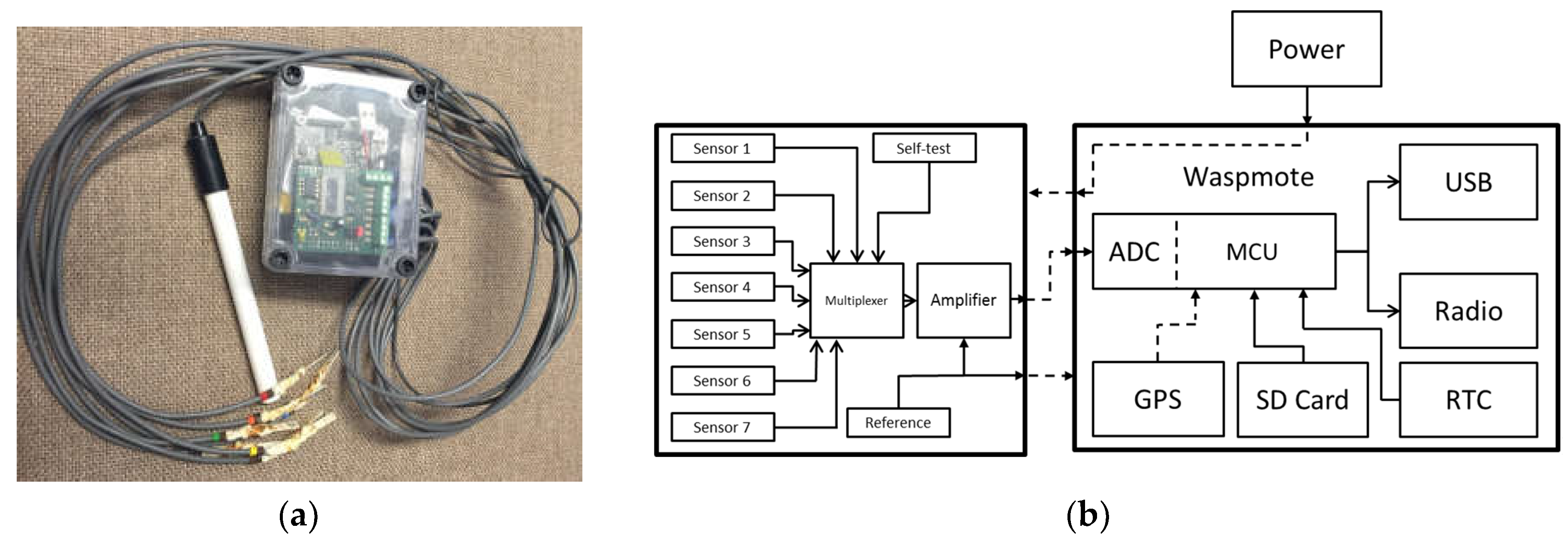
Figure 2.
Schematic illustration of the potentiometric sensor construction.

Figure 3.
Photograph of measured channel section for Neerigen Brook Reach 1. Arrow pointing downstream. (picture: K. Smettem)
Figure 3.
Photograph of measured channel section for Neerigen Brook Reach 1. Arrow pointing downstream. (picture: K. Smettem)

Figure 4.
Neerigen Brook Reach 1. Cross-section tracer curves. Legend shows distance across channel transect and mid-channel EC data.
Figure 4.
Neerigen Brook Reach 1. Cross-section tracer curves. Legend shows distance across channel transect and mid-channel EC data.

Figure 5.
Photograph of measured channel section for Neerigen Brook Reach 2. Arrow pointing downstream. (picture K. Smettem)
Figure 5.
Photograph of measured channel section for Neerigen Brook Reach 2. Arrow pointing downstream. (picture K. Smettem)
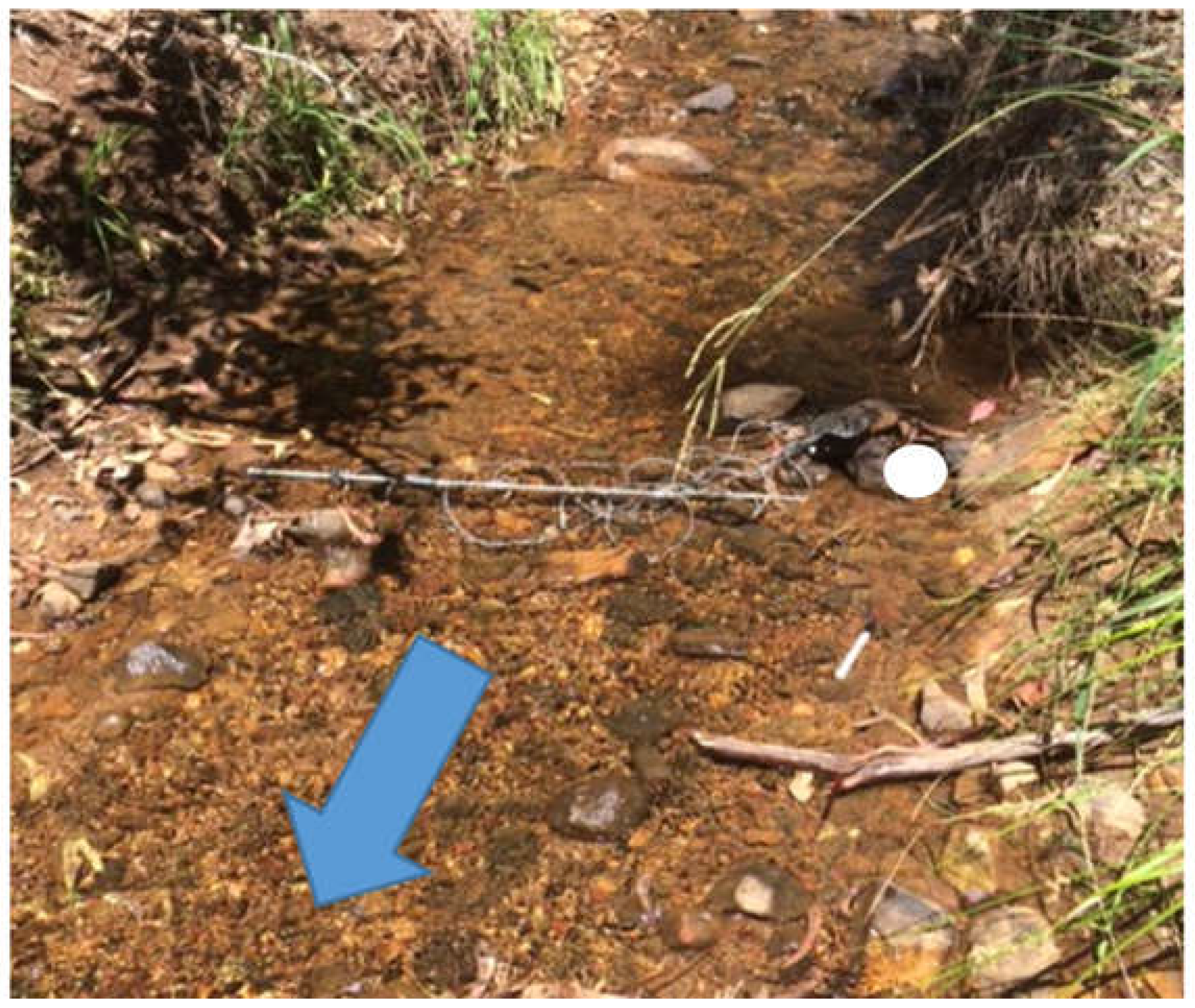
Figure 6.
Chloride concentration curves measured across Neerigen Brook Reach 2. Legend shows distance across channel transect and mid-channel EC data.
Figure 6.
Chloride concentration curves measured across Neerigen Brook Reach 2. Legend shows distance across channel transect and mid-channel EC data.

Figure 7.
(a). Photograph of the measured channel section for the Weierbach. Arrow pointing downstream (picture J. Klaus); (b). Cross-section schematic of the Weierbach channel showing positions of exposed rocks and chloride sensors.
Figure 7.
(a). Photograph of the measured channel section for the Weierbach. Arrow pointing downstream (picture J. Klaus); (b). Cross-section schematic of the Weierbach channel showing positions of exposed rocks and chloride sensors.
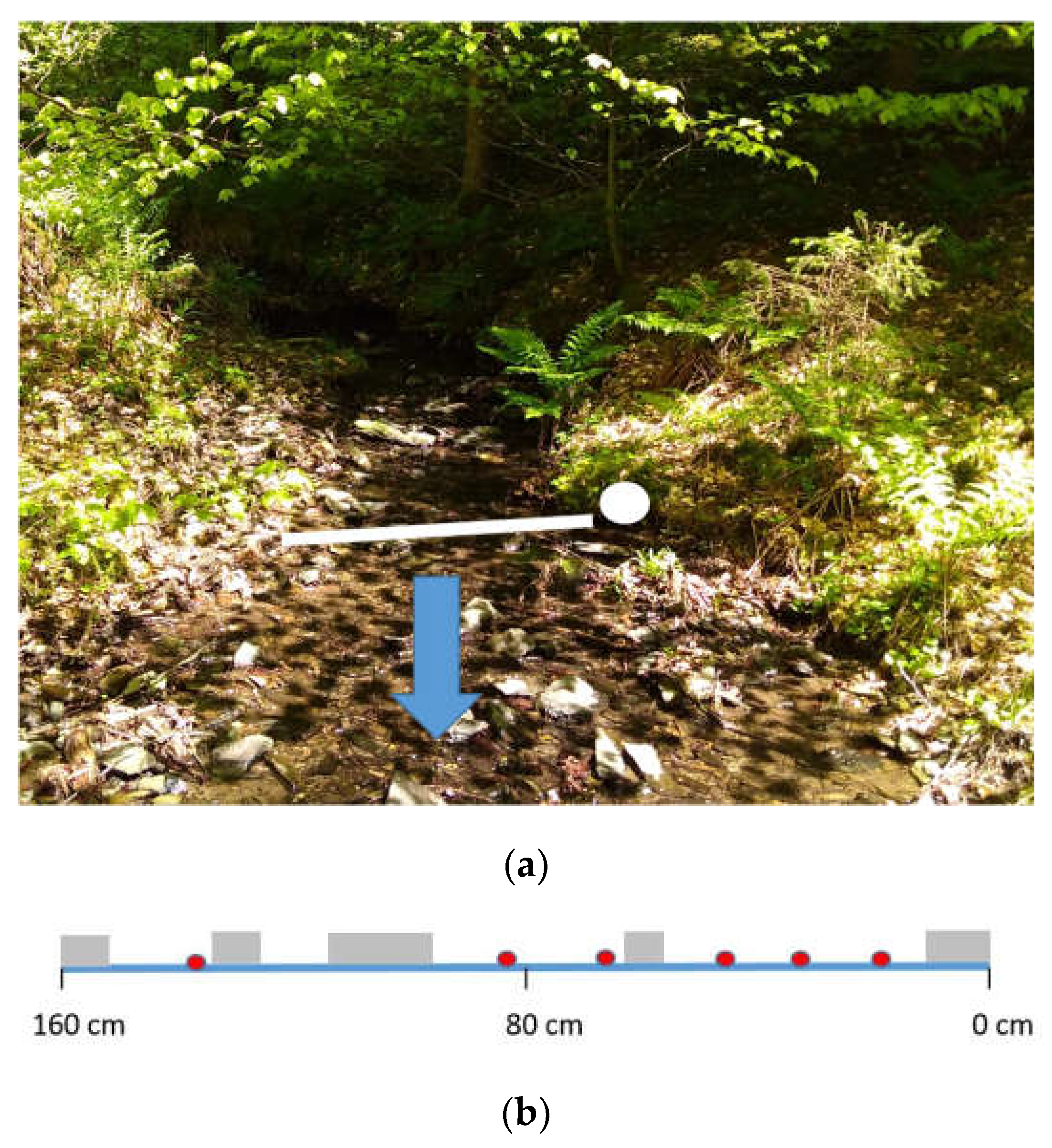
Figure 8.
Chloride concentration curves measured across the Weierbach. Legend shows distance across channel transect and mid-channel EC data.
Figure 8.
Chloride concentration curves measured across the Weierbach. Legend shows distance across channel transect and mid-channel EC data.
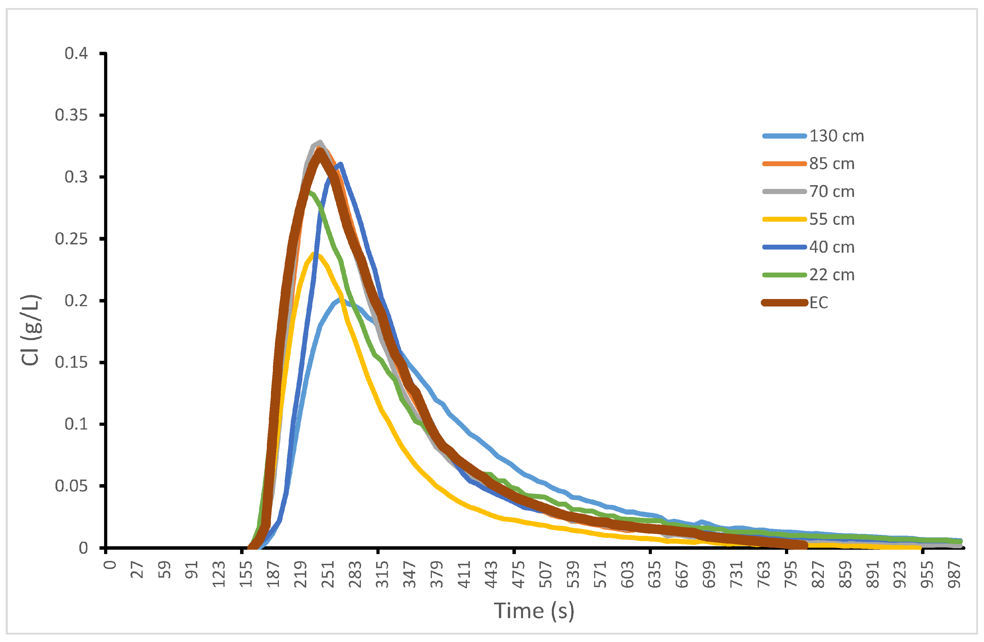
Figure 9.
Photograph of the measured channel section for the Koulbich. (picture J. Klaus)

Figure 10.
(a) Koulbich cross-channel tracer concentration profile. Red line is data converted from the mid-channel EC probe; (b) Tracer concentration versus time contours across the Koulbich transect.
Figure 10.
(a) Koulbich cross-channel tracer concentration profile. Red line is data converted from the mid-channel EC probe; (b) Tracer concentration versus time contours across the Koulbich transect.

Figure 11.
Photograph of measured channel section across the Rennbach-Koulbich confluence. Arrow pointing downstream. (picture M. Antonelli)
Figure 11.
Photograph of measured channel section across the Rennbach-Koulbich confluence. Arrow pointing downstream. (picture M. Antonelli)
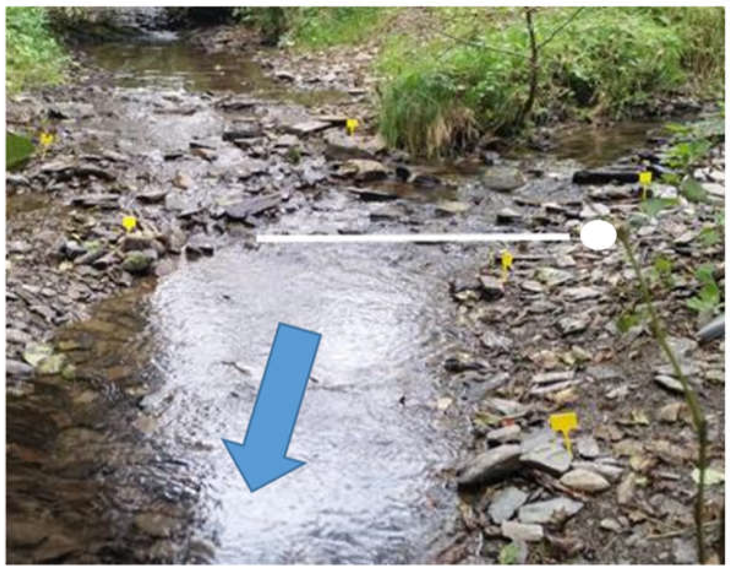
Figure 12.
(a) Rennbach-Koulbich mixing zone cross-channel tracer concentration profile. Red line is data converted from the mid-channel EC probe; (b) Tracer concentration versus time contours across the Rennbach-Koulbich mixing zone transect.
Figure 12.
(a) Rennbach-Koulbich mixing zone cross-channel tracer concentration profile. Red line is data converted from the mid-channel EC probe; (b) Tracer concentration versus time contours across the Rennbach-Koulbich mixing zone transect.

Table 1.
Study reach characteristics, tracer injection details and bed conditions.
| Stream Name | Reach Length (m) | Mean Channel Width (m) | Discharge (m3/s) | Mean Flow Rate (m/s) | Injected Tracer Mass Per Trace (g) | Channel Bed Conditions |
|---|---|---|---|---|---|---|
| Neerigen Brook Reach 1 | 25.0 | 0.75 | 0.015 | 0.2 | 300 (2 traces) 200 (1 trace) | Straight riffle section, no exposed bed. |
| Neerigen Brook Reach 2 | 44.0 | 1.30 | 0.018 | 0.11 | 300 (3 traces) | Riffle-pool sequence with exposed rocks |
| Weierbach | 19.5 | 1.55 | 0.003 | 0.085 | 50 (2 traces) | Highly braided riffle pool sequence |
| Koulbich | 45.0 | 0.85 | 0.067 | 0.50 | 500 (1 trace) 1000 (3 traces) | Straight riffle section upstream from eroded near bank pool |
| Rennbach | 15.0 | 0.75 * | 0.048 | 0.064 | 500 (4 traces) | Riffle pool sequence running into channel confluence. |
* Width prior to confluence with Koulbich.
Table 2.
Neerigen Brook Reach 1. Tracer results for skewness and time to peak.
| Distance Across Channel | 10 cm | 20 cm | 30 cm | 40 cm | 55 cm | 65 cm | EC Probe |
|---|---|---|---|---|---|---|---|
| Skew | |||||||
| run 1 | 0.76 | 0.65 | 0.66 | 0.85 | 0.77 | 1.15 | 0.84 |
| run 2 | 1.05 | 0.85 | 0.88 | 1.06 | 1.09 | 1.01 | 0.82 |
| run 3 | 1.10 | 0.98 | 0.93 | 1.06 | 0.82 | 0.98 | 0.78 |
| Time to peak (s) | |||||||
| run 1 | 126 | 126 | 126 | 117 | 126 | 126 | 125 |
| run 2 | 117 | 126 | 126 | 126 | 126 | 126 | 125 |
| run 3 | 126 | 126 | 126 | 126 | 126 | 135 | 125 |
Table 3.
Neerigen Brook Reach 2. Tracer results for skewness and time to peak.
| Distance Across Channel | 40 cm | 60 cm | 75 cm | 90 cm | 105 cm | 120 cm | EC Probe |
|---|---|---|---|---|---|---|---|
| Skew | |||||||
| run 1 | 1.00 | 0.89 | 1.06 | 1.08 | 1.02 | 1.01 | 0.81 |
| run 2 | 1.05 | 0.85 | 0.88 | 1.06 | 1.08 | 1.01 | 0.87 |
| run 3 | 1.01 | 0.99 | 0.93 | 1.10 | 0.82 | 0.98 | 0.83 |
| Time to peak (s) | |||||||
| run 1 | 423 | 432 | 405 | 378 | 396 | 396 | 400 |
| run 2 | 414 | 405 | 387 | 387 | 396 | 405 | 400 |
| run 3 | 383 | 423 | 387 | 387 | 396 | 396 | 400 |
Table 4.
Weierbach. Tracer results for skewness and time to peak.
| Distance Across Channel | 22 cm | 40 cm | 55 cm | 70 cm | 85 cm | 130 cm | EC Probe |
|---|---|---|---|---|---|---|---|
| Skew | |||||||
| run 1 | 0.84 | 1.40 | 1.49 | 1.53 | 1.51 | 1.35 | 1.29 |
| run 2 | 0.98 | 1.49 | 1.50 | 1.31 | 1.86 | 1.54 | 1.35 |
| Time to peak (s) | |||||||
| run 1 | 219 | 267 | 235 | 243 | 243 | 267 | 235 |
| run 2 | 219 | 243 | 235 | 243 | 251 | 267 | 235 |
Table 5.
Koulbich. Tracer results for skewness and time to peak.
| Distance Across Channel | 12 cm | 24 cm | 36 cm | 48 cm | 56 cm | 64 cm | 76 cm | EC Probe |
|---|---|---|---|---|---|---|---|---|
| Skew | ||||||||
| run 1 | 1.62 | 1.33 | 0.88 | 1.10 | 1.35 | 1.24 | 1.35 | 1.08 |
| run 2 | 1.50 | 1.87 | 1.62 | 1.75 | 1.57 | 1.40 | 1.78 | 1.07 |
| run 3 | 1.52 | 1.10 | 1.54 | 1.76 | 1.63 | 1.63 | 1.57 | 0.88 |
| Time to peak (s) | ||||||||
| run 1 | 90 | 90 | 81 | 90 | 90 | 99 | 90 | 90 |
| run 2 | 90 | 90 | 81 | 90 | 99 | 99 | 99 | 90 |
| run 3 | 90 | 90 | 81 | 81 | 90 | 99 | 81 | 90 |
Table 6.
Rennbach-Koulbich mixing zone. Tracer results for skewness and time to peak.
| Distance Across Channel | 12 cm | 24 cm | 36 cm | 48 cm | 56 cm | 64 cm | 76 cm | EC Probe |
|---|---|---|---|---|---|---|---|---|
| Skew | ||||||||
| run 1 | 0.49 | 0.59 | 0.63 | 0.54 | 0.58 | 0.59 | 0.52 | 0.45 |
| run 2 | 0.49 | 0.52 | 0.62 | 0.49 | 0.49 | 0.65 | 0.50 | 0.47 |
| run 3 | 0.12 | 0.17 | 0.25 | 0.17 | 0.13 | 0.25 | 0.13 | 0.44 |
| run 4 | 0.56 | 0.51 | 0.50 | 0.52 | 0.21 | 0.20 | 0.13 | 0.45 |
| Time to peak (s) | ||||||||
| run 1 | 247 | 229 | 220 | 229 | 247 | 247 | 265 | 235 |
| run 2 | 247 | 238 | 229 | 238 | 265 | 247 | 247 | 235 |
| run 3 | 238 | 238 | 229 | 238 | 256 | 238 | 238 | 235 |
| run 4 | 238 | 229 | 229 | 238 | 247 | 238 | 247 | 235 |
© 2017 by the authors. Licensee MDPI, Basel, Switzerland. This article is an open access article distributed under the terms and conditions of the Creative Commons Attribution (CC BY) license (http://creativecommons.org/licenses/by/4.0/).
Share and Cite
MDPI and ACS Style
Smettem, K.; Klaus, J.; Harris, N.; Pfister, L. New Potentiometric Wireless Chloride Sensors Provide High Resolution Information on Chemical Transport Processes in Streams. Water 2017, 9, 542. https://doi.org/10.3390/w9070542
AMA Style
Smettem K, Klaus J, Harris N, Pfister L. New Potentiometric Wireless Chloride Sensors Provide High Resolution Information on Chemical Transport Processes in Streams. Water. 2017; 9(7):542. https://doi.org/10.3390/w9070542
Chicago/Turabian StyleSmettem, Keith, Julian Klaus, Nick Harris, and Laurent Pfister. 2017. "New Potentiometric Wireless Chloride Sensors Provide High Resolution Information on Chemical Transport Processes in Streams" Water 9, no. 7: 542. https://doi.org/10.3390/w9070542
Note that from the first issue of 2016, this journal uses article numbers instead of page numbers. See further details here.