Influencing Factors and Simplified Model of Film Hole Irrigation

Abstract

Film hole irrigation is an advanced low-cost and high-efficiency irrigation method, which can improve water conservation and water use efficiency. Given its various advantages and potential applications, we conducted a laboratory study to investigate the effects of soil texture, bulk density, initial soil moisture, irrigation depth, opening ratio (ρ), film hole diameter (D), and spacing on cumulative infiltration using SWMS-2D. We then proposed a simplified model based on the Kostiakov model for infiltration estimation. Error analyses indicated SWMS-2D to be suitable for infiltration simulation of film hole irrigation. Additional SWMS-2D-based investigations indicated that, for a certain soil, initial soil moisture and irrigation depth had the weakest effects on cumulative infiltration, whereas ρ and D had the strongest effects on cumulative infiltration. A simplified model with ρ and D was further established, and its use was then expanded to different soils. Verification based on seven soil types indicated that the established simplified double-factor model effectively estimates cumulative infiltration for film hole irrigation, with a small mean average error of 0.141–2.299 mm, a root mean square error of 0.177–2.722 mm, a percent bias of −2.131–1.479%, and a large Nash–Sutcliffe coefficient that is close to 1.0.

1. Introduction

Severe global water shortages have attracted ample attention because water is crucial for human beings, particularly in agriculture [1,2,3]. Notably, the arid and semiarid regions of the western part of China have encountered serious water scarcity problems because of limited rainfall and great soil-moisture evaporation [4,5]. The use of advanced water-saving irrigation methods, such as sprinkler irrigation, microsprinkler irrigation, surface drip irrigation, and subsurface drip irrigation, is encouraged, particularly in these arid and semiarid areas of China with high rates of evaporation. However, the cost of advanced irrigation systems is relatively high for farmers in underdeveloped areas [6]. Therefore, a low-cost and efficient irrigation method is urgently required.

Currently, plastic mulching has become a globally applied agricultural practice for high yields and increased water-use efficiency. This method is primarily used to protect seedlings in arid climates, prevent evaporation, maintain or slightly increase soil temperature and humidity, prevent weed growth, and reduces herbicide and fertilizer use [7,8,9,10,11,12]. These prospects have increased the immediate relevance of plastic film technology; currently, plastic films constitute the largest proportion of agricultural surface coverings [13,14]. According to the National Bureau of Statistics of China [15], China is the world’s largest film mulch consumer and boasts the world’s largest film mulch coverage area. The area covered by film mulch considerably increased to 20 million hm² in 2014, and its use increased fourfold (from 642 to 2580 megatons) from 1991 to 2014. Film hole irrigation has also developed along with film-mulched techniques for crops with wide line spacing [16]. Film hole irrigation is a relatively new irrigation method that involves completely covering a bordered field with plastic film with holes of uniform size [17]. Water penetrates into the soil through the holes during irrigation, and seedlings sprout through these holes on germination. Compared with the traditional surface irrigation method, this technique considerably reduces water losses and improves the uniformity of irrigation along the long direction of the border [6,16,18,19].

Mathematical models and software, such as winSRFR [20], have been widely used in the design of irrigation systems to improve the efficiency of water application and the uniformity of water distribution. Film hole irrigation is somewhat similar to point-source irrigation, in that water infiltration occurs in the region directly around the film hole. Unlike other point source irrigation systems, in which the water is transported by tubes, in film mulch irrigation, water is applied to the top of the border or furrow and it flows above the applied film mulch to the end of the border or furrow under the influence of gravity, similar to surface irrigation. In the design of a surface irrigation system, a zero-inertia model and winSRFR software are the most useful tools. In the model, the infiltration and roughness are the key parameters to be determined. As with surface irrigation, the infiltration characteristics of film hole irrigation are fundamental for determining a field film hole irrigation scheme with high application efficiency and distribution uniformity. Therefore, studying a simple and easily-estimated infiltration model of film hole irrigation is essential. Numerous laboratory studies and some field studies on film hole infiltration have been conducted in the last two decades in China; such studies have mainly focused on wetting patterns, empirical modeling, and infiltration characteristics, including single and multipoint source infiltration [18,21,22]. However, the models of all of these studies have been empirical descriptions of some specific soils; therefore, a more universally applicable model must be developed.

Numerical simulation is often used in soil research. From a theoretical point of view, film hole irrigation involves three-dimensional point-source infiltration under a low-pressure water head (i.e., irrigation depth). Similar to subsurface drip irrigation, film hole infiltration is affected by many factors, such as soil texture, bulk density (γ_d), irrigation depth, film hole diameter (D), and hole spacing (i.e., distance between the centers of two neighboring holes). With the development of computer simulation techniques, numerical simulations based on the theory of unsaturated soil water movement are being increasingly used to study soil water infiltration. Several programs, such as HYDRUS and SWMS-2D, are often used to simulate soil water movement, and these have been effectively and accurately applied to subsurface drip irrigation [23,24,25,26,27,28] for predicting wetting patterns and infiltration characteristics, yielding more generally applicable results [29].

Therefore, the objectives of this study were: (1) to assess the feasibility of SWMS-2D for simulation of the cumulative infiltration of film hole irrigation through a laboratory experiment; (2) to investigate the effects of various influencing factors on cumulative infiltration in film hole irrigation and then to select the dominant factors; and (3) to propose and verify a simplified double-factor model that estimates the infiltration of film hole irrigation.

2. Materials and Methods

2.1. Laboratory Experiments

Given the realities that constrain film hole irrigation in the field, the film hole diameters and spacing are generally determined by the actual situation of field crops. The diameters of film holes and the spaces between them are typically 3–8 and 12–30 cm, respectively. The opening ratio, ρ, is defined as the ratio of the area of the open holes to the total area under the plastic mulching; in general, ρ is 2–5%; the irrigation amount is 225–450 m³·hm⁻²; and the irrigation depth relative to the film mulch is kept constant within a range of 4–6 cm [30,31]. The soil is usually irrigated when the soil water content (SWC) is at 40–60% field capacity. Considering all of these irrigation variables, we designed eight treatments for our experiments (

Table 1. Test scheme for film hole irrigation.

Treatment	Soil Type *	Bulk Density (g/cm3)	Distance between Film Holes (cm)	Hole Diameter (cm)	Initial Water Content ** (%)	Irrigation Depth (cm)	Irrigation Amount (m3/hm2)	Irrigation Volume *** (mL)
1	Silt loam	1.30	20	4	40	4	225	900
2		1.40	20	4	60	6	450	1800
3		1.30	30	6	60	6	225	2025
4		1.40	30	6	40	4	450	4050
5	Sandy loam	1.35	30	4	60	4	450	4050
6		1.45	30	4	40	6	225	2025
7		1.35	20	6	40	6	450	1800
8		1.45	20	6	60	4	225	900

Notes: * Based on the USDA Soil Taxonomy System; ** Initial water content is the percentage of field capacity; *** Irrigation volume represents the irrigation volume of water supplied within the controlling area of a single hole in the experimental setup.

).

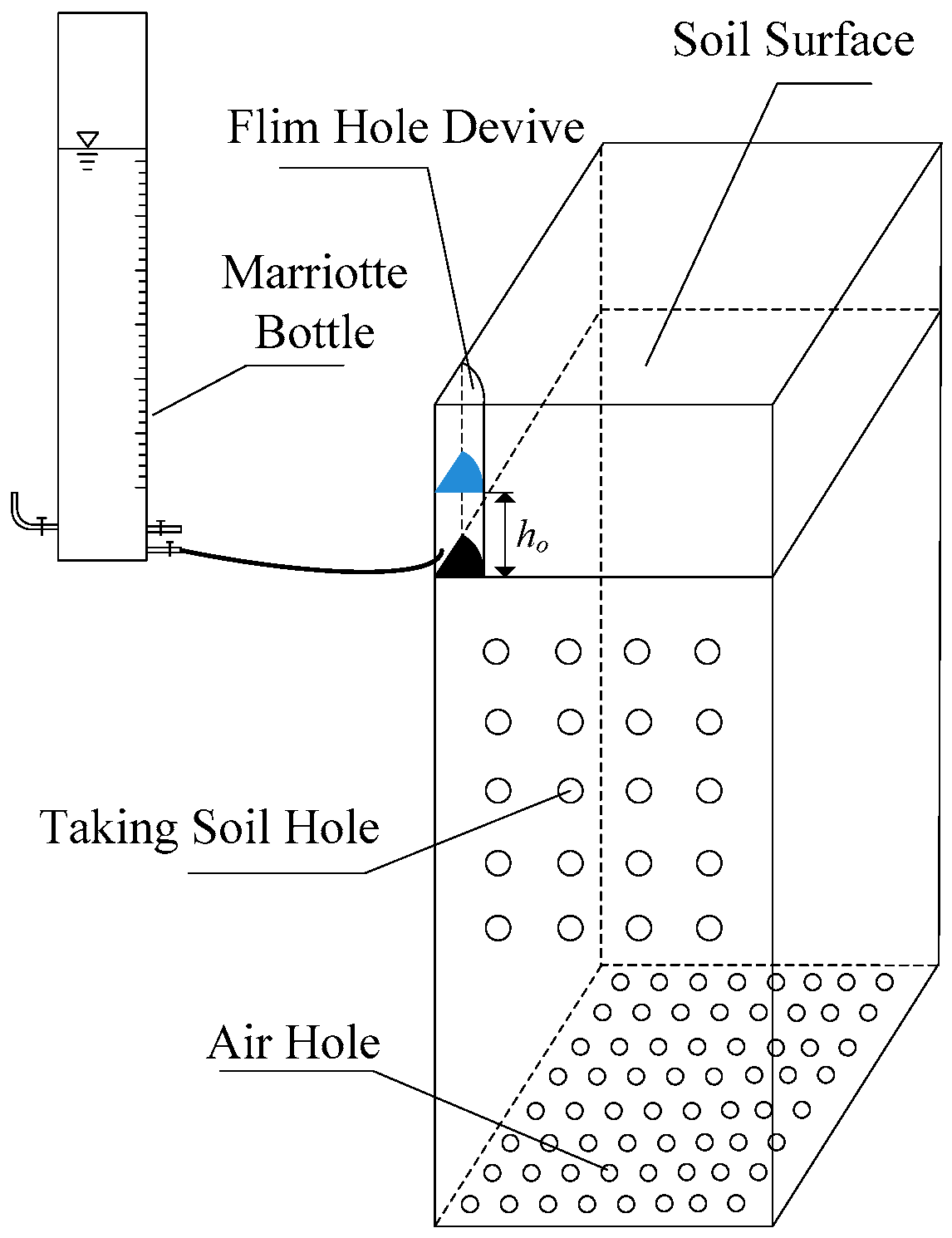
Figure 1 illustrates the laboratory setup for the experiments. Considering the symmetry characteristics of film hole infiltration, two soil bins, composed of 10-mm-thick transparent acrylic material, were designed; one of these bins measured 10 cm in length, 10 cm in width, and 60 cm in depth; the other was 15 cm in length, 15 cm in width, and 60 cm in depth. The bottom of each soil bin had numerous 2-mm parallel air vents for ventilation, and on both sides of the bins were side holes for soil sampling for SWC measurement; the diameter of each hole and the spaces between the holes were 1.5 and 5 cm, respectively. Before the soil was filled into the soil bin, transparent adhesive tape was placed on both sides of the soil bin to prevent the soil from falling out of the box. A Marriotte vessel was used to maintain a constant hydraulic head.

Silt loam and sandy loam (based on the USDA Soil Taxonomy System) from Yangling District, China, were used for the experiments. The particle size distributions of the silt loam were 13.52% 0–0.002 mm, 79.23% 0.002–0.02 mm, and 7.25% 0.02–2 mm, while those of the sandy loam were 3.10% 0–0.002 mm, 42.63% 0.002–0.02 mm, and 54.27% 0.02–2 mm. The soil samples were collected from the 20–60-cm depths of a field. Soil samples were air-dried, sieved through a 2-mm mesh, and then compacted into the soil bin at bulk densities of 1.30, 1.35, 1.40, and 1.45 g·cm⁻³ to simulate the in situ bulk density. Some water was added to the dry soil and mixed with the soil before filling the soil bin to reach the experimental desired initial SWC values of the eight treatments. The soil was loaded and compacted in the bin in 5-cm layers to obtain a homogeneous soil profile. To maintain zero evaporation, the soil surface was covered with a polyethylene sheet. Based on the design of the experiments, the irrigation volume of a single hole could be determined; accordingly, an infiltration depth of 4–6 cm was maintained by the Marriotte bottle. Cumulative infiltration was recorded during the infiltration. Finally, soil samples were collected from side holes and SWC was determined by recording the weight loss of the samples after oven drying at 105 °C for 24 h.

2.2. Numerical Model Establishment and Calibration

Because film hole irrigation can be simplified as a process of point-source water infiltration, water movement during infiltration can be considered as an axisymmetric three-dimensional infiltration process. The following partial differential equation based on the Richards equation governs water flow through variably unsaturated media:

$$\frac{\partial \theta }{\partial t}=\frac{\partial }{\partial r}\left[K(\phi )\frac{\partial \phi }{\partial r}\right]+\frac{K(\phi )}{r}\frac{\partial \phi }{\partial r}+\frac{\partial }{\partial z}\left[K(\phi )(\frac{\partial \phi }{\partial z}-1)\right],$$

(1)

where $\theta$ is the soil water content (cm³·cm⁻³); $\phi$ is the potential head (cm); $K(\phi )$ is the hydraulic conductivity (cm·min⁻¹); z is the depth from the soil surface (cm), measured with positive values in the downward direction; r is the radial coordinate (cm); and t is the time (min).

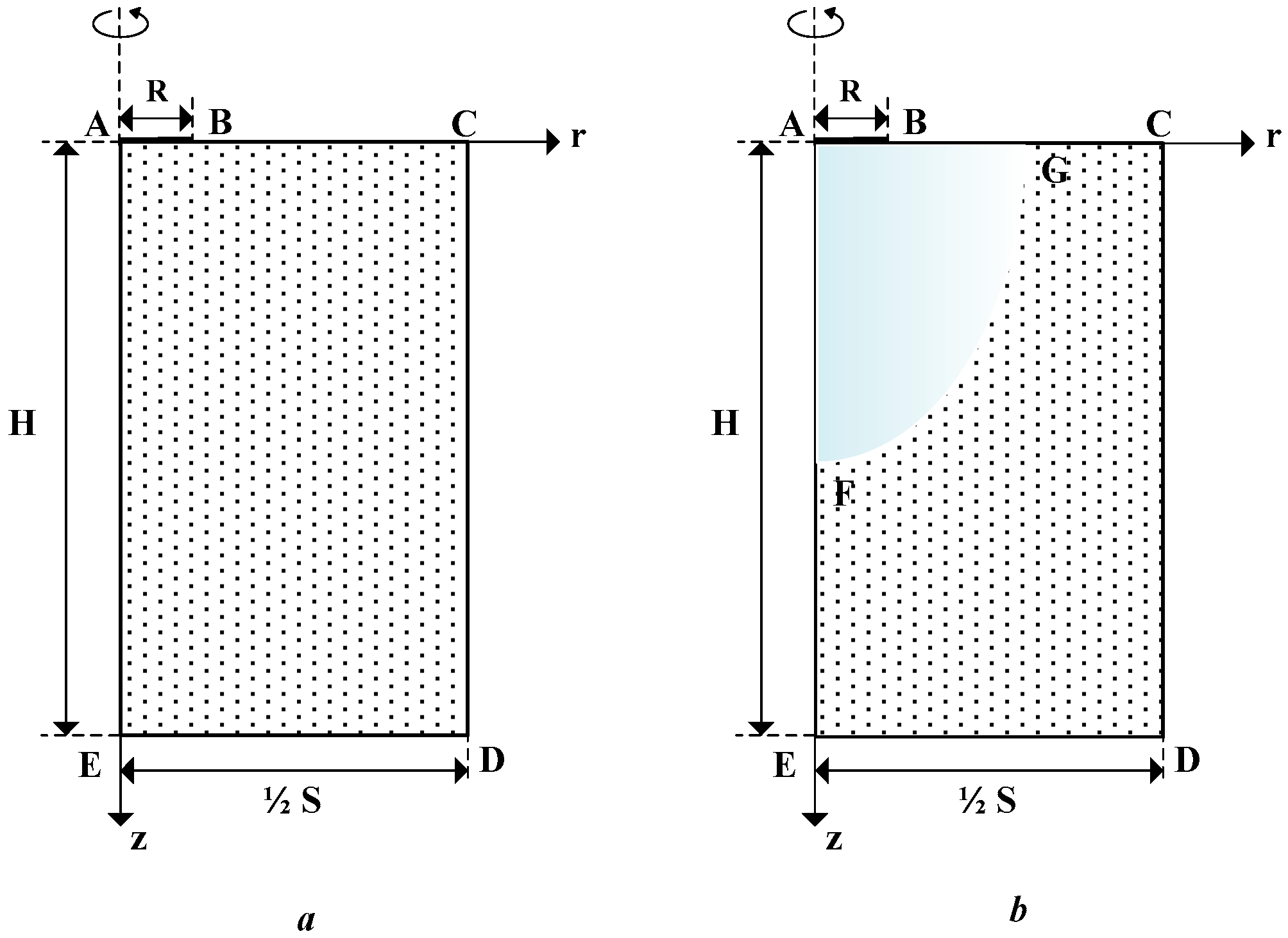
The infiltration space can be described as a three-dimensional axisymmetric domain, as shown in Figure 2a. With the infiltration process, water moves into the inner soil; the wetting pattern is shown in Figure 2b.

SWMS-2D under the axisymmetric three-dimensional flow model was used to solve the point source infiltration process of film hole irrigation [23]. The initial conditions of the system are as follows:

$$\phi ={\phi }_0, 0\le r\le 1/2 S, 0\le z\le H, t=0,$$

(2)

where ${\phi }_0$ is the initial water potential before irrigation (cm⁻¹); R and S are the radius and space of the film hole (cm), respectively; and H is the depth of simulation domain (cm).

The boundary AB is the surface through which water enters with a water head of h₀ (Equation (3)). The boundary BC, covered with plastic mulch, with no infiltration or evaporation, is the zero-flux boundary, as shown in Equation (4). The boundaries AE and CD are partially symmetric boundaries without exchange of water flow in the r direction; they are also zero-flux boundaries, as shown in Equations (5) and (6). The boundary ED constitutes the bottom and is not affected by infiltration; therefore, it has a fixed initial soil water potential, as shown in Equation (7).

$$\phi =h_0, z=0, 0\le r\le R, t\ge 0,$$

(3)

$$K(\phi )\left[\frac{\partial \phi }{\partial z}-1\right]=0, z=0, R\le r\le 1/2^{} S, t\ge 0,$$

(4)

$$K(\phi )\frac{\partial \phi }{\partial r}=0, 0\le z\le H, r=0, t\ge 0,$$

(5)

$$K(\phi )\frac{\partial \phi }{\partial r}=0, 0\le z\le H, r=1/2^{} S, t\ge 0,$$

(6)

$$\phi ={\phi }_0, z=H, 0\le r\le 1/2^{} S, t\ge 0,$$

(7)

The water retention curve and hydraulic conductivity curve are important soil characteristics [32]. A centrifugal machine (SCR-20) was used to obtain a water retention curve under rotational speeds of 900, 1700, 2200, 2800, 3100, 5300, 6900, and 8100 rpm; each speed was maintained for 1 h. Then, SWC was measured for each rotational speed, whereupon the capillary head was calculated from Equation (8) [33].

$$h=1.118\times {10}^{-5}\times R_0\times {(\mathrm{rpm})}^2$$

(8)

where R₀ is the radial distance to the midpoint of the soil sample (cm).

The van Genuchten–Mualem model was used to describe the curves of soil water retention, θ(φ), and of hydraulic conductivity, K(θ):

$$\theta \left(\phi \right)={\theta }_r+\frac{{\theta }_s-{\theta }_r}{{\left(1+{\left|\alpha \phi \right|}^n\right)}^m},$$

(9)

$$K(\theta )=K_s{S}_e{}^l{\left[1-{(1-S_e^{\raisebox{1ex}{$1$}\!\left/ \!\raisebox{-1ex}{$m$}\right.})}^m\right]}^2,$$

(10)

$$S_e=\frac{\theta -{\theta }_r}{{\theta }_s-{\theta }_r},$$

(11)

$$D(\theta )=K(\theta )\cdot \frac{d\phi }{d\theta }$$

(12)

where θ_r and θ_s are the residual and saturated water contents (cm³·cm⁻³), respectively; K(θ) is the saturated hydraulic conductivity (cm·min⁻¹); D(θ) is the soil diffusivity, which is obtained by horizontal column infiltration method (cm²·min⁻¹); α is an empirical parameter that is inversely related to the air-entry pressure value (cm⁻¹); n is an empirical parameter related to the pore-size distribution; l is an empirical shape parameter; m = 1 − 1/n; and S_e is the effective saturation.

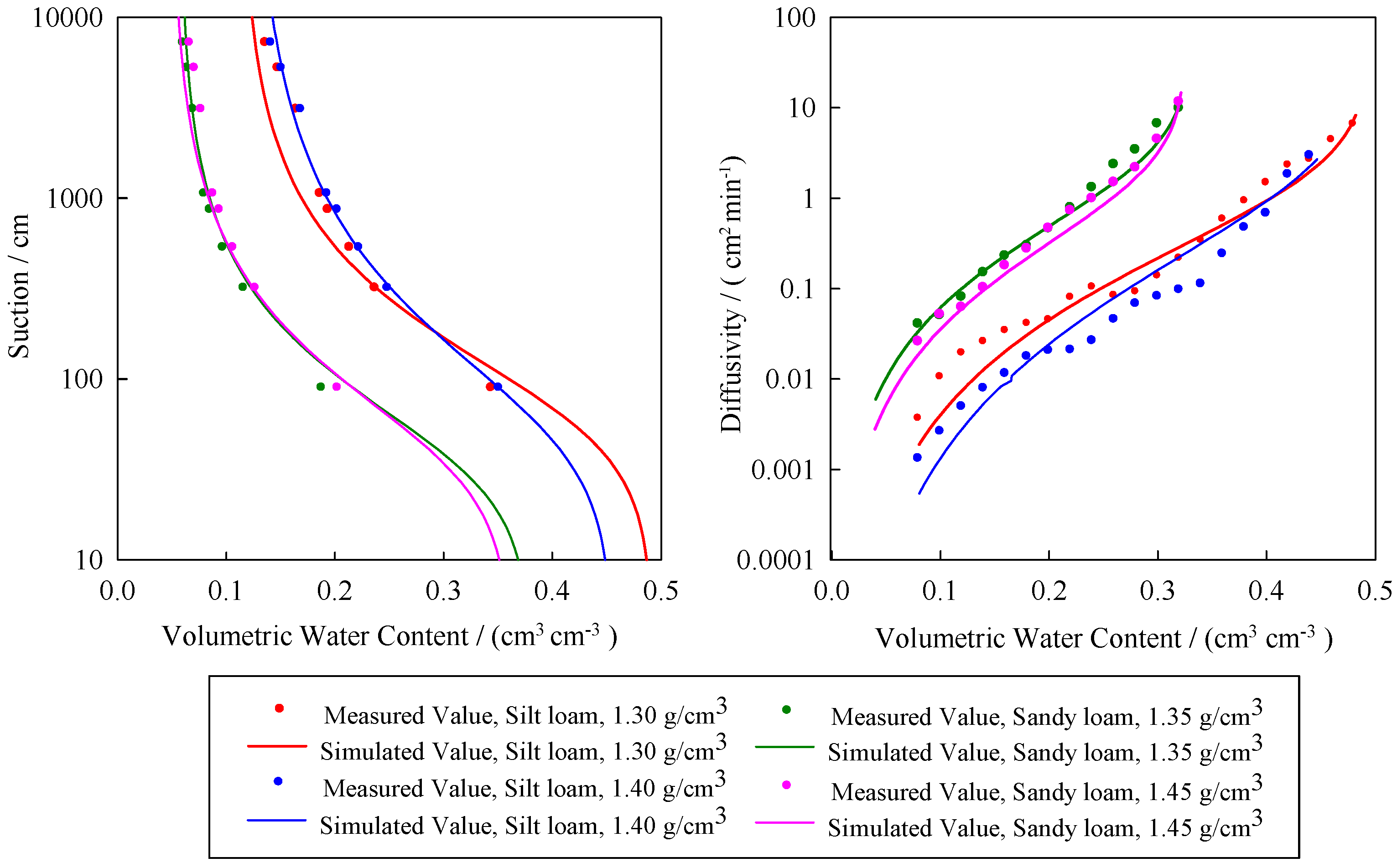
The experimental data of soil water retention and diffusivity were fitted to the van Genuchten–Mualem model by using the RETC code [34,35]. The parameters of the van Genuchten–Mualem model are listed in

Table 2. Parameters for the van Genuchten–Mualem model of experimental soils.

Soil Type	Bulk Density (g/cm3)	θr (cm3/cm3)	θs (cm3/cm3)	α (1/cm)	n	l	Ks (cm/min)
Silt loam	1.30	0.113	0.492	0.014	1.72	0.5	0.0208
	1.40	0.123	0.456	0.017	1.55	0.5	0.0154
Sandy loam	1.35	0.057	0.38	0.025	1.76	0.5	0.0409
	1.45	0.049	0.362	0.024	1.69	0.5	0.0257
Sand	-	0.045	0.430	0.145	2.68	0.5	0.4950
Sandy loam	-	0.065	0.410	0.075	1.89	0.5	0.0737
Loam	-	0.078	0.430	0.036	1.56	0.5	0.0173
Loamy sand	-	0.057	0.040	0.124	2.28	0.5	0.2432
Silt	-	0.034	0.460	0.016	1.37	0.5	0.0042
Silt loam	-	0.067	0.450	0.020	1.41	0.5	0.0075
Sandy clay loam	-	0.100	0.390	0.059	1.48	0.5	0.0218
Clay loam	-	0.095	0.410	0.019	1.31	0.5	0.0043
Silty clay loam	-	0.089	0.430	0.001	1.23	0.5	0.0012

. A comparison of fitted soil water retention and diffusivity curves by model and measured data is shown in Figure 3.

The van Genuchten–Mualem model parameters for 11 selected types of soil, including silt loam, sandy loam, sand, sandy loam, loam, loamy sand, silt, silt loam, sandy clay loam, clay loam, and silty clay loam, were obtained using RETC software [35] and are listed in Table 2.

2.3. Simplified Kostiakov Model for Film Hole Infiltration

The cumulative infiltration and duration were described using the Kostiakov model given as Equation (13). In this study, six influencing factors for film hole irrigation were analyzed. Moreover, dominant factors were selected, and a simplified equation based on the Kostiakov model for film hole infiltration would be further proposed.

$$I=k{t}^{\alpha }$$

(13)

where I is the cumulative infiltration (mm), t is the infiltration duration (min), k is an infiltration coefficient (mm min⁻¹), and α is the infiltration index.

2.4. Error Analysis

Four indicators, namely mean absolute error (MAE), root mean squared error (RMSE), percent bias (PBIAS), and Nash–Sutcliffe coefficient (NS), were selected to make error analyses between the measured and simulated values of SWC and cumulative infiltration.

$$\mathrm{MAE}=\frac{{{\displaystyle \sum }}_1^n\left|Y_i^{sim}-Y_i^{obs}\right|}{n}$$

(14)

$$\mathrm{RMSE}=\sqrt{\frac{1}{n-1}{\displaystyle \sum }_{i=1}^n{\left(Y_i^{sim}-Y_i^{obs}\right)}^2},\mathrm{for} i=1,2\dots n$$

(15)

$$\mathrm{PBIAS}=\frac{{{\displaystyle \sum }}_{i=1}^n\left(Y_i^{sim}-Y_i^{obs}\right)}{{{\displaystyle \sum }}_{i=1}^n{Y}_i^{obs}}$$

(16)

$$\mathrm{NS}=1-\frac{{{\displaystyle \sum }}_{i=1}^n{\left(Y_i^{sim}-Y_i^{obs}\right)}^2}{{{\displaystyle \sum }}_{i=1}^n{(Y_i^{obs}-{\overline{Y}}_i^{obs})}^2}$$

(17)

where n is the total number of data points in each case,.$Y_i^{\mathit{sim}}$ is the ith simulated datum, and $Y_i^{obs}$ is the ith measured datum. The MAE can potentially identify the presence of bias. The RMSE provides an overall measure of the degree to which the data differ from the model predictions, whereas the PBIAS is the deviation of data being evaluated, expressed as a percentage. If PBIAS within ±10%, the PBIAS values are considered to be within a very accurate range. A value of 1 for the NS means the simulated value is as accurate as the measured value [36].

3. Results and Discussion

3.1. Application of SWMS-2D to Film Hole Irrigation and Comparison with the Experimental Results

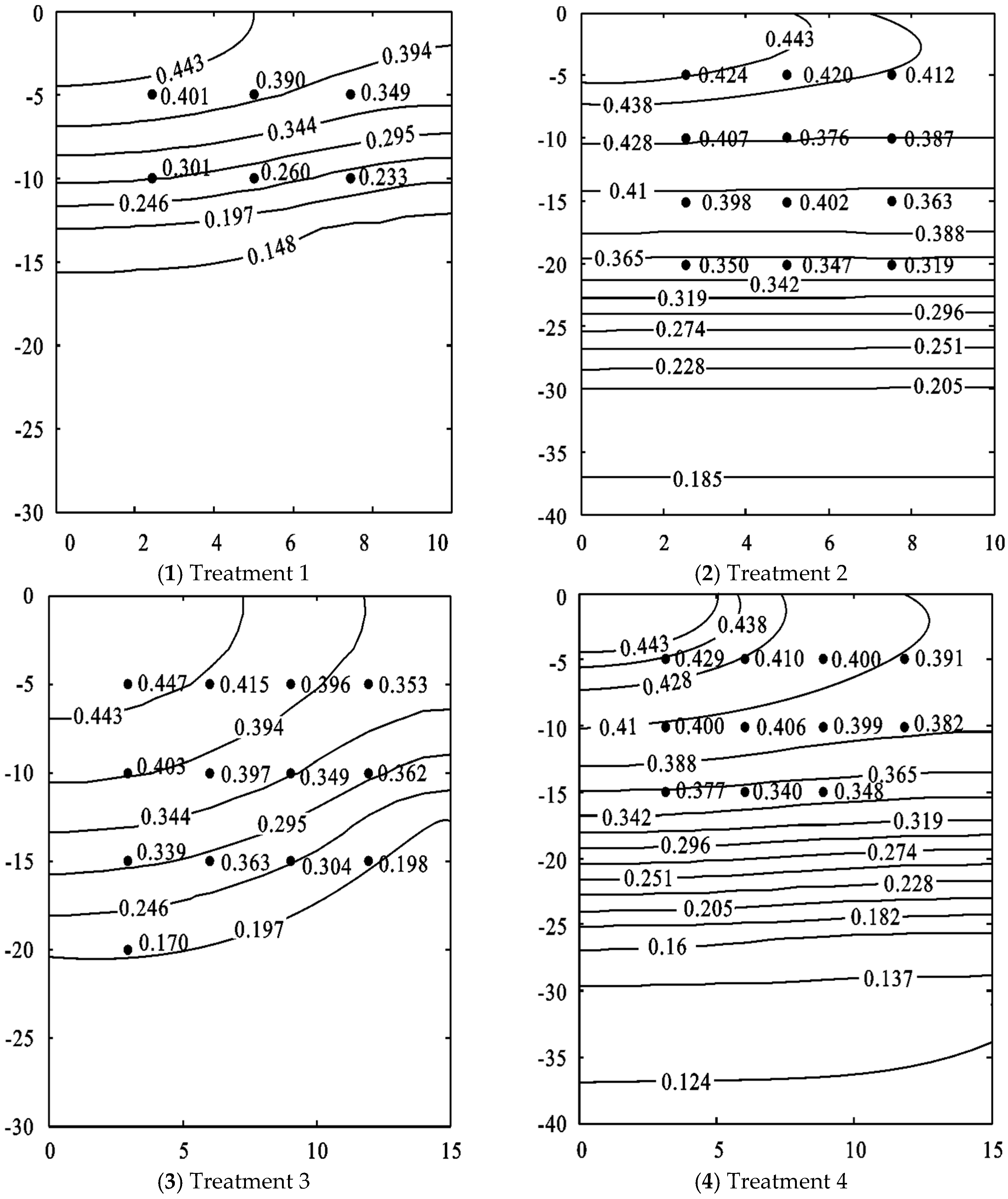
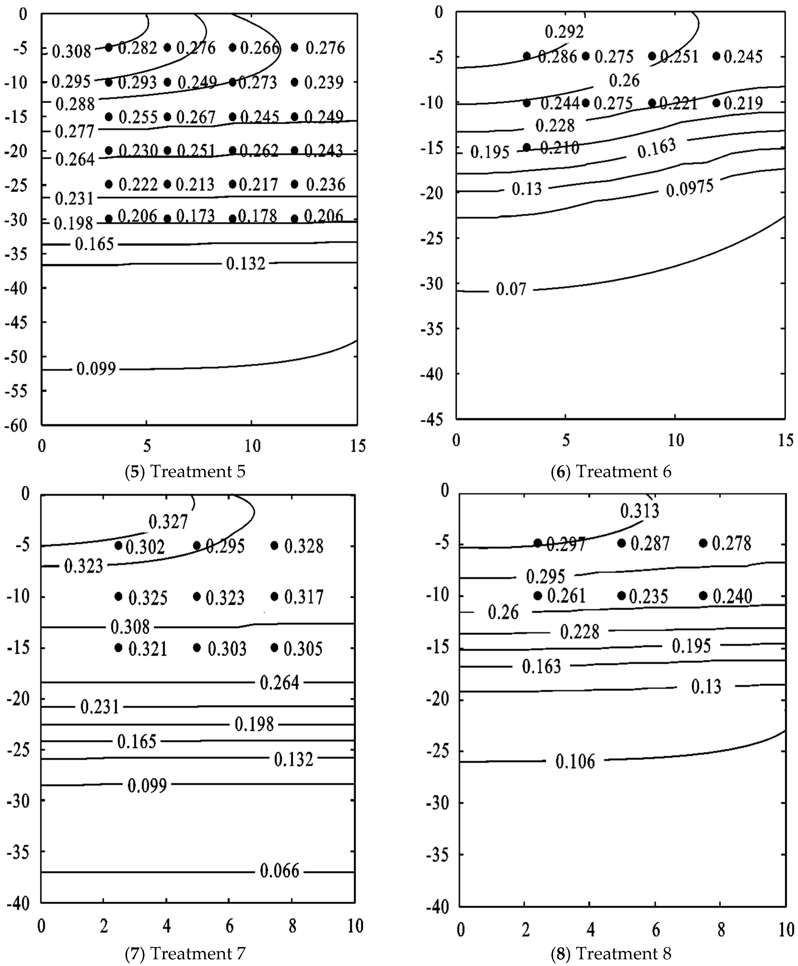
Figure 4 shows the measured and simulated SWC distribution data for the eight treatments in Table 1. The measured SWC is represented by black dots, whereas simulation results obtained through SWMS-2D are shown as contour lines. The MAE, RMSE, PBIAS, and NS values for measured and simulated SWC are presented in

Table 3. Correlation between simulated and measured SWC levels.

Treatment	MAE (cm3/cm3)	RMSE (cm3/cm3)	PBIAS (%)	NS
1	0.013	0.016	2.947	0.979
2	0.022	0.028	2.711	0.998
3	0.026	0.034	3.648	0.997
4	0.011	0.013	1.962	0.995
5	0.020	0.023	3.508	0.968
6	0.011	0.013	1.438	0.998
7	0.013	0.016	0.461	0.998
8	0.026	0.028	2.762	0.999

; the results indicated the SWMS-2D model to be suitable for describing soil water distributions resulting from film hole irrigation, because it had extremely small MAE, RMSE, and PBIAS values (1.091–2.600 cm³·cm⁻³, 0.013–0.034 cm³·cm⁻³, and 0.461–3.648%, respectively), and a large NS (very close to 1.0).

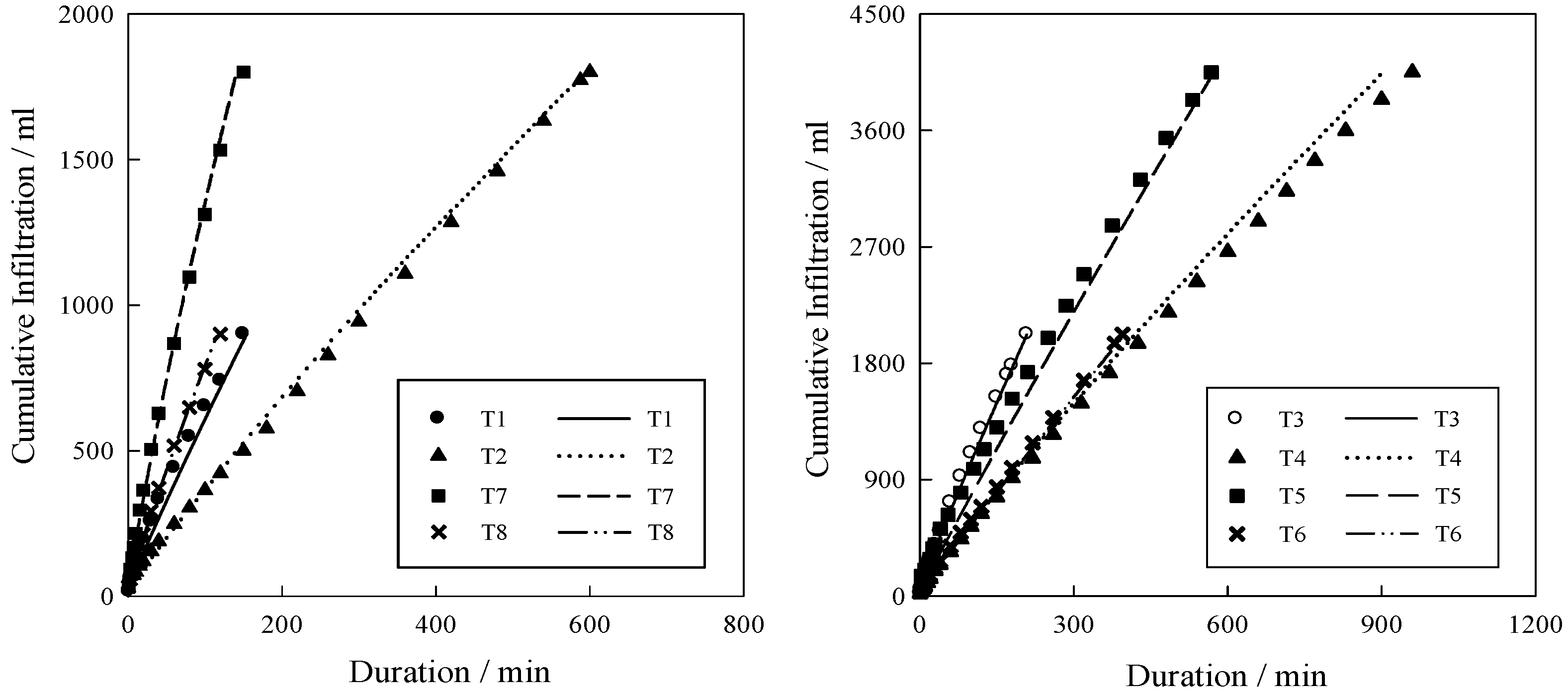
Figure 5 compares simulated and measured cumulative infiltration values for different treatments. The simulated values agreed reasonably well with the measured values, with small PBIAS values from −0.197% to 0.914% and large NS values from 0.989 to 0.999, which indicated that the SWMS-2D model can effectively simulate cumulative infiltration resulting from film hole irrigation.

3.2. Different Factors Affecting Cumulative Infiltration of Film Hole Irrigation

3.2.1. Effect of Initial SWC on Cumulative Infiltration

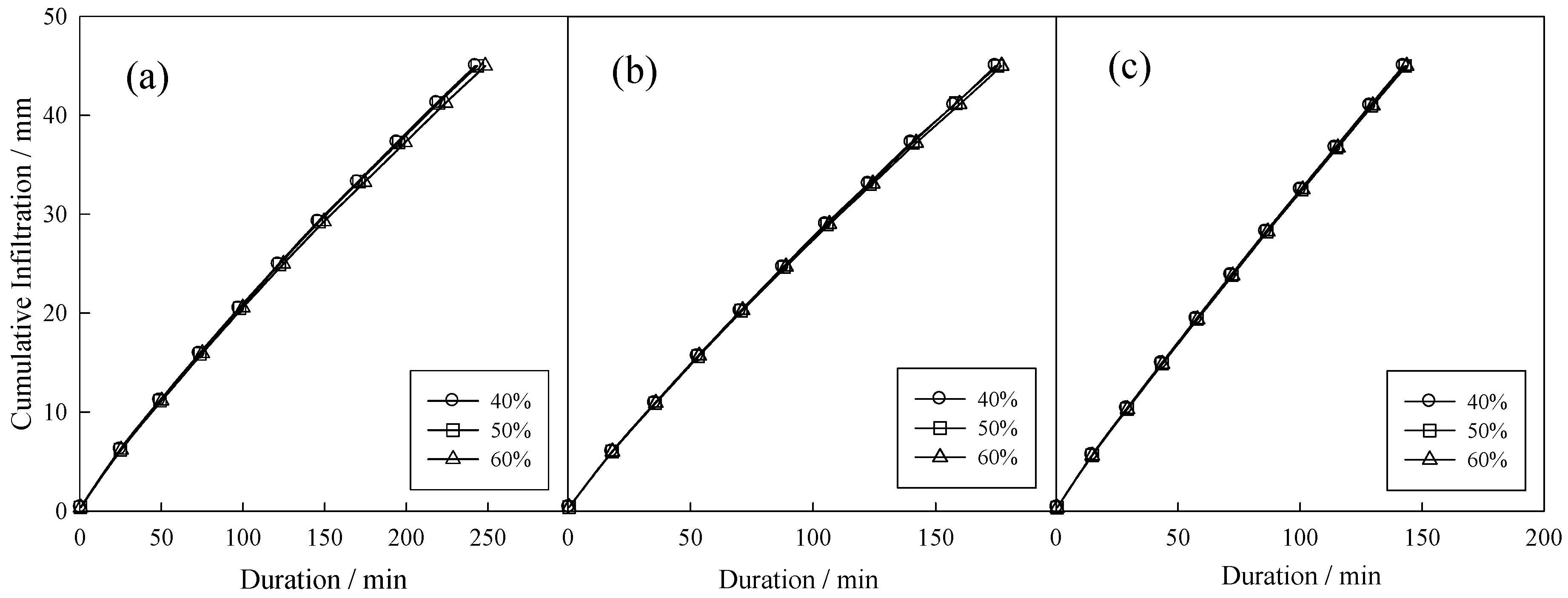
Simulations of three soil types, namely silt loam (γ_d = 1.30 g·cm⁻³), sandy loam (γ_d = 1.35 g·cm⁻³), and loamy sand (simulated on the basis of information obtained from RETC software), were executed at different initial SWC levels with a film hole diameter of 5 cm, spacing of 20 cm, irrigation depth of 6 cm, and irrigation amount of 450 m³·hm⁻². The field capacities of the silt loam, sandy loam, and loamy sand were 0.243, 0.126, and 0.160 cm³·cm⁻³, respectively. The cumulative infiltration curves of the film holes at different initial SWC levels are shown in Figure 6; the initial SWC had little effect on the cumulative infiltration dynamic of a single film hole. As the SWC increased, the water potential gradient slightly decreased, leading to a slight decrease in cumulative infiltration. Therefore, the impacts of initial SWC could be ignored in film hole irrigation research.

3.2.2. Effect of Irrigation Depth on Cumulative Infiltration

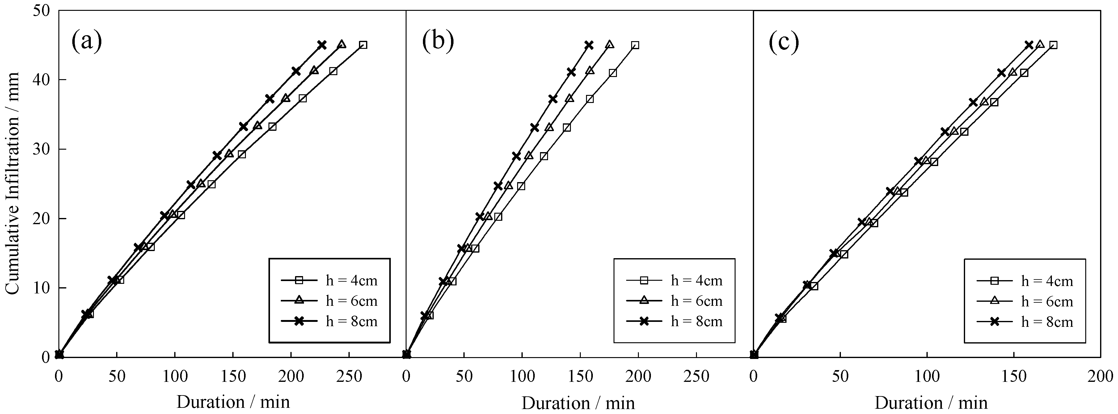
Figure 7 illustrated the effects of different irrigation depths in the silt loam, sandy loam, and loamy sand. All simulations were conducted at a film hole diameter of 5 cm, film hole spacing of 20 cm, initial SWC of 50% field water capacity, and irrigation amount of 450 m³·hm⁻². The irrigation depth had little effect on the film hole infiltration characteristics (Figure 7). As the irrigation depth increased, the film hole infiltration rate slightly increased. However, because the value of gravity potential caused by irrigation depth was so small, relative to matrix potential that changes of gravity potential at different irrigation depths was smaller, that it can be ignored. Accordingly, because of the slight changes in film hole infiltration at different irrigation depths, the infiltration was disregarded in later investigations.

3.2.3. Effect of Layered-Soil Depth on Cumulative Infiltration

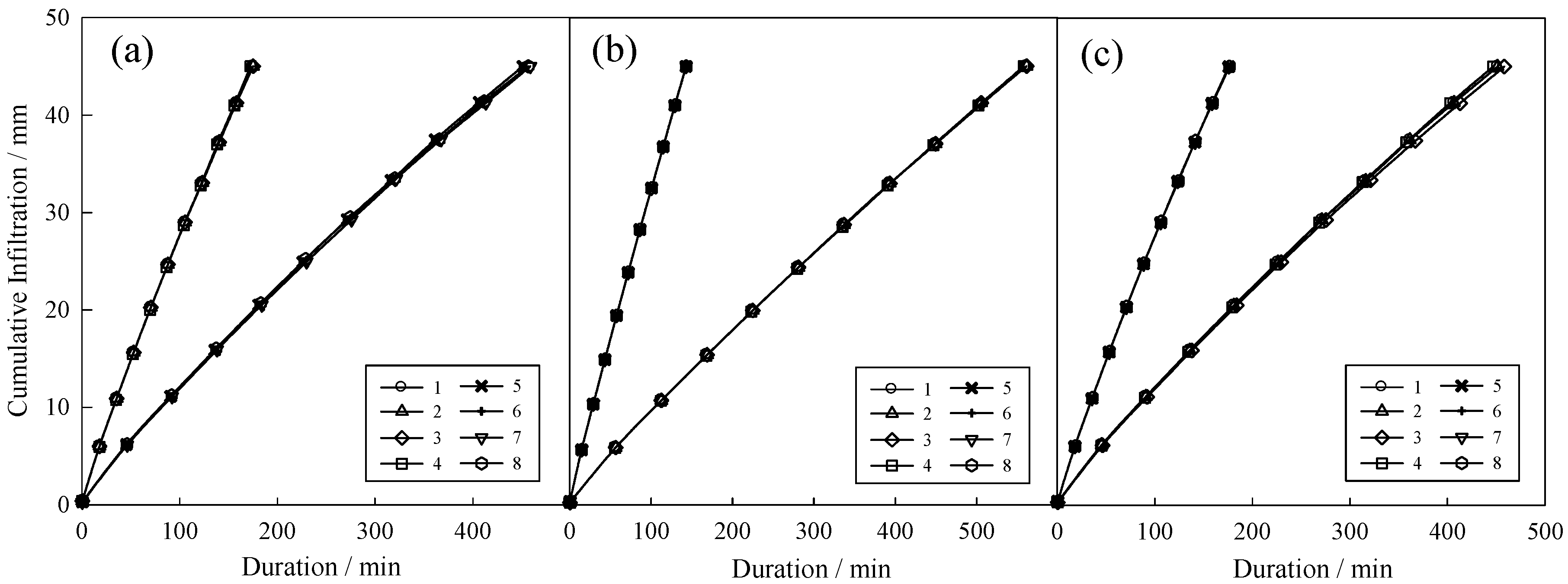
To consider the actual soil conditions in the field, and to analyze the effect of upper soil depth on film hole infiltration, this study conducted simulations of six cases of layered soil. Different soil types and bulk densities were obtained at various upper soil depths. Homogeneous soils and upper soils with 15-, 20-, and 30-cm-deep soil layers were simulated for all cases. Case 1 involved sandy loam (1.35 g·cm⁻³) on top with silt loam (1.30 g·cm⁻³) underneath. Case 2 involved silt loam (1.40 g·cm⁻³) on top with sandy loam (1.45 g·cm⁻³) underneath. Case 3 involved loamy sand on top with loam underneath. Case 4 involved loam on top with loamy sand underneath. Cases 5 and 6 involved combinations of the same soil types but with different bulk densities: Case 5 considered silt loam soil with bulk densities of 1.40 and 1.30 g·cm⁻³, whereas Case 6 considered sandy loam with bulk densities of 1.35 and 1.45 g·cm⁻³. As illustrated in Figure 8, the hydraulic characteristics of the soil at the lower layers (at depths beyond 15 cm) had no significant effect on cumulative infiltration, which was predominantly affected by the characteristics of the soil at the upper layers. In other words, the upper soil characteristics predominantly affected film hole infiltration characteristics under film hole irrigation with the normal amount of water. Thus, the soil at depths of 0–15 cm has the dominant influence on the cumulative infiltration of layered soil.

3.2.4. Effect of Film Hole Diameter and Opening Ratio on Cumulative Infiltration

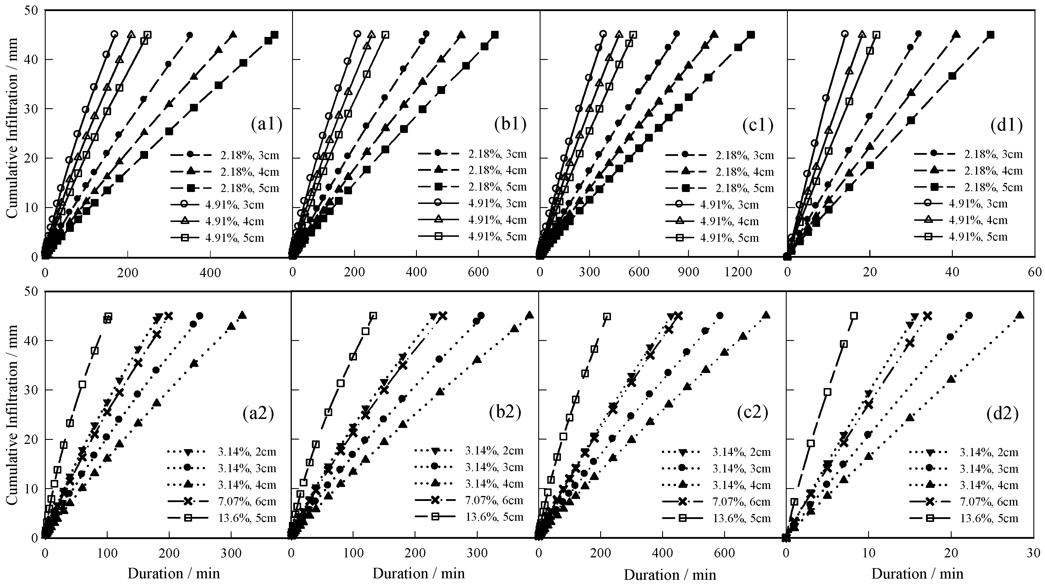
Silt loam (γ_d = 1.30 g·cm⁻³), sandy loam (γ_d = 1.45 g·cm⁻³), loam, and sand were selected to simulate cumulative infiltration of film hole irrigation under different D and ρ values. The simulations were conducted at a film hole spacing of 20 cm, an irrigation water depth of 6 cm, an initial SWC of 50% field capacity, and an irrigation amount of 450 m³·hm⁻². As shown in Figure 9, for all treatments, the cumulative infiltration increased as ρ increased, but decreased as D increased under the same ρ; in addition, sand had the highest infiltration rate, followed by loam and sandy loam. From the above analysis, the effects of D and ρ should be taken into account in film hole irrigation research.

3.3. Establishment and Universality of a Simplified Model

3.3.1. Establishment of a Simplified Model

This study selected 11 soil types, including silt loam (γ_d = 1.30 and 1.40 g·cm⁻³) and sandy loam (γ_d = 1.35 and 1.45 g·cm⁻³) as well as other sandy, loam, and silt soils, to analyze the characteristics of film hole infiltration. Cumulative infiltration was simulated at a film hole diameter of 5 cm, spacing of 20 cm, irrigation water depth of 6 cm, and irrigation amount of 450 m³·hm⁻².

Equation (13) was used to fit the relationship between k and α, listed in

Table 4. Fitted infiltration parameter values.

Opening Ratio (%)	Film Hole Diameter (cm)	Silt Loam		Silt Loam		Sandy Loam		Sandy Loam		Loam		Sand		Sandy Loam
		(γd = 1.30 g/cm3)		(γd = 1.40 g/cm3)		(γd = 1.35 g/cm3)		(γd = 1.45 g/cm3)
		k	α	k	α	k	α	k	α	k	α	k	α	k	α
2.18	3	0.2553	0.877	0.1636	0.858	0.2919	0.901	0.199	0.89	0.1247	0.866	1.5957	0.96	0.3166	0.923
	4	0.2104	0.871	0.135	0.853	0.2325	0.902	0.161	0.888	0.105	0.861	1.281	0.955	0.2658	0.912
	5	0.1811	0.866	0.1155	0.852	0.1987	0.901	0.138	0.886	0.0928	0.854	1.0895	0.95	0.2327	0.904
	Mean	0.2156	0.871	0.138	0.855	0.241	0.901	0.166	0.888	0.1075	0.86	1.3221	0.955	0.2717	0.913
3.14	2	0.5242	0.858	0.3354	0.839	0.6107	0.875	0.414	0.865	0.2503	0.849	3.2732	0.954	0.6146	0.923
	3	0.3825	0.861	0.2466	0.841	0.4345	0.885	0.298	0.873	0.186	0.852	2.3225	0.953	0.4627	0.915
	4	0.3164	0.856	0.2052	0.836	0.3469	0.888	0.243	0.873	0.1582	0.846	1.8665	0.948	0.3912	0.903
	Mean	0.4077	0.858	0.2624	0.839	0.464	0.883	0.318	0.87	0.1982	0.849	2.4874	0.951	0.4895	0.913
4.91	3	0.6265	0.835	0.4062	0.815	0.7098	0.857	0.448	0.846	0.303	0.83	3.6961	0.937	0.7405	0.899
	4	0.5152	0.834	0.335	0.815	0.5732	0.863	0.397	0.851	0.2558	0.828	2.9535	0.937	0.6232	0.891
	5	0.4495	0.83	0.294	0.813	0.4959	0.862	0.346	0.849	0.2321	0.82	2.5265	0.932	0.5543	0.881
	Mean	0.5304	0.833	0.3451	0.814	0.593	0.861	0.397	0.849	0.2636	0.826	3.0587	0.935	0.6393	0.89
7.07	6	0.6129	0.806	0.4041	0.788	0.6652	0.84	0.467	0.827	0.3208	0.796	3.2753	0.916	0.7475	0.859
13.6	5	1.408	0.855	0.9345	0.737	1.5422	0.776	1.087	0.768	0.7197	0.759	7.3773	0.863	1.6553	0.828
Opening Ratio (%)	Film Hole Diameter (cm)	Loamy Sand		Silt		Silt Loam		Sandy Clay Loam		Clay Loam		Silt Clay Loam
		k	α	k	α	k	α	k	α	k	α	k		α
2.18	3	0.7757	0.967	0.0311	0.905	0.0445	0.923	0.0789	0.946	0.0236	0.922	0.0989		0.805
	4	0.6049	0.969	0.0258	0.898	0.0426	0.896	0.0619	0.946	0.0247	0.886	0.1071		0.752
	5	0.4996	0.973	0.0194	0.915	0.0314	0.917	0.0491	0.956	0.0152	0.93	0.0441		0.861
	Mean	0.6268	0.969	0.0255	0.906	0.0395	0.912	0.0633	0.95	0.0212	0.913	0.0833		0.806
3.14	2	1.6726	0.944	0.1024	0.827	0.1384	0.847	0.1731	0.924	0.0683	0.861	0.3556		0.686
	3	1.2272	0.952	0.0605	0.864	0.0877	0.878	0.1277	0.931	0.0474	0.879	0.2041		0.737
	4	0.9004	0.96	0.0358	0.903	0.0555	0.91	0.0941	0.937	0.0329	0.896	0.1171		0.791
	Mean	1.2668	0.952	0.0662	0.865	0.0939	0.879	0.1316	0.931	0.0495	0.879	0.2256		0.738
4.91	3	1.8915	0.932	0.1062	0.833	0.15	0.848	0.2123	0.904	0.0801	0.851	0.3878		0.678
	4	1.4747	0.941	0.0709	0.864	0.1104	0.867	0.1662	0.911	0.0634	0.86	0.2464		0.726
	5	1.2257	0.947	0.0581	0.872	0.0914	0.874	0.1355	0.919	0.0518	0.868	0.1781		0.754
	Mean	1.5306	0.94	0.0784	0.856	0.1173	0.863	0.1713	0.912	0.0651	0.86	0.2708		0.719
7.07	6	1.6189	0.929	0.0856	0.847	0.1336	0.848	0.1858	0.902	0.0762	0.843	0.2581		0.720
13.6	5	4.0632	0.846	0.3217	0.738	0.4536	0.746	0.5099	0.838	0.2412	0.763	0.9397		0.580

, for different soils. The correlation coefficients (R²) for all soils were all larger than 0.99, indicating that the Kostiakov model can adequately describe the relationship between cumulative infiltration and duration.

Based on the preceding analysis, with the same soil texture and the same bulk density as actual field film hole irrigation, the initial SWC and irrigation depth weakly affected cumulative infiltration. Therefore, D and ρ were viewed as the two main influencing factors in model establishment for a given soil. The values of k increased with ρ, but decreased with increased D under the same ρ. The values of α decreased with ρ, and had no significant relationship with D. After extensive verification, Equations (18) and (19) were proposed based on the relationships among k, α, ρ, and D.

$$k=A\frac{{\rho }^m}{D^n},$$

(18)

$$\alpha =B-\eta \rho ,$$

(19)

where k is the infiltration coefficient (mm min⁻¹); ρ is the opening ratio (%); D is the film hole diameter (cm); and A, m, n, B, and η are the fitting parameters.

Based on the k and α data for all soil samples listed in Table 4, the model parameters A, B, m, n, and η were fitted using MATLAB, and the values of m, n, and η were 1.131, 0.698, and 0.997 (where 0.997 can be considered as effectively equal to 1.0), respectively; and A and B varied with soil texture and bulk density. Therefore, Equation (13) was reconstructed using a combination of D and ρ as follows:

$$I=A(\frac{{\rho }^{1.131}}{D^{0.698}})t^{B-\rho }$$

(20)

3.3.2. Evaluation of the Simplified Model Universality

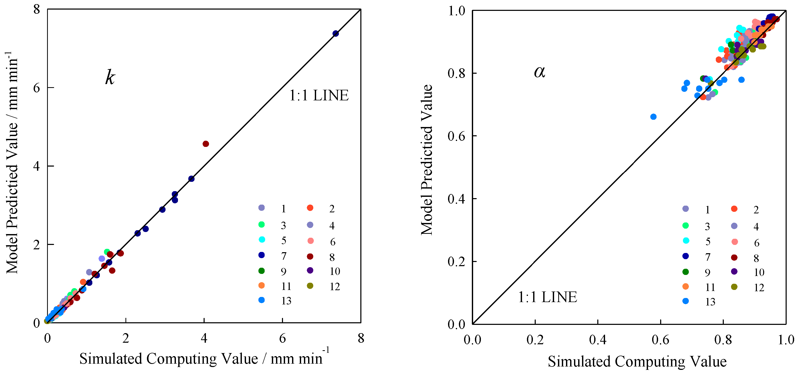
Table 4 compares parameters k and α for different soil texture and bulk densities; their estimated values based on Equations (18) and (19) are shown in Figure 10. The simulated values of k and α were in good agreement with almost all estimated values, indicating that the simplified model, Equation (20), is suitable for infiltration estimation for various soils with different D and ρ values. In addition, α was observed to be numerically stable at approximately 0.9; however, this requires further analysis.

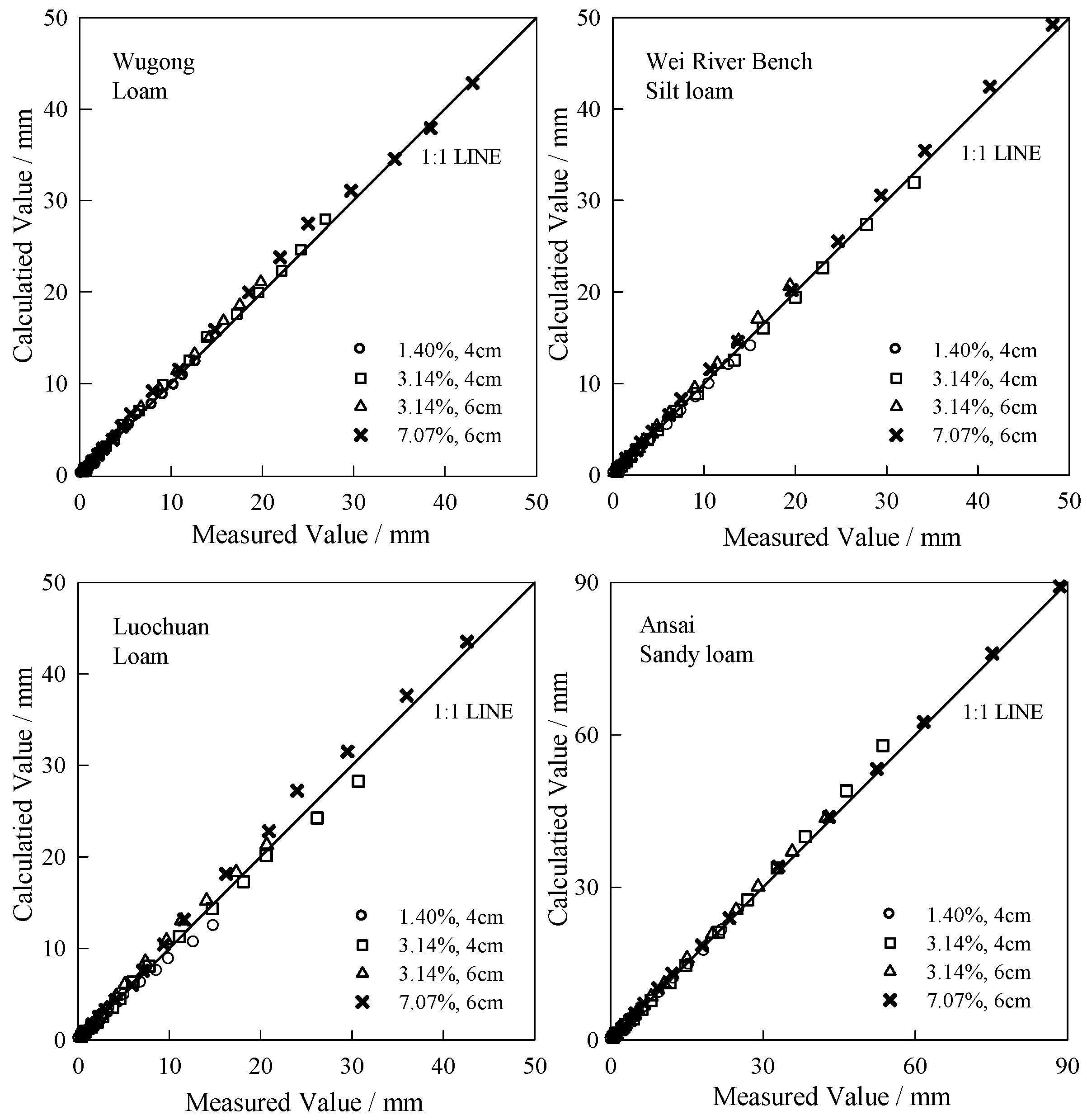
The experiment results, including four soil types located in different regions on the Loess Plateau, China, which were loam from Wugong (γ_d = 1.30 g·cm⁻³), silt loam from Wei River Bench (γ_d = 1.45 g·cm⁻³), loam from Luochuan (γ_d = 1.40 g·cm⁻³) and sandy loam from Ansai (γ_d = 1.35 g·cm⁻³) [37], were used to verify the universality of the simplified model. The infiltration models were obtained based on Equation (20). As presented in Figure 11, the calculated values obtained from Equations (21)–(24) were well matched with the experimental values, signifying that the simplified model of Equation (20) can effectively describe the characteristics of film hole infiltration.

$$I=42.94({\rho }^{1.131}/D^{0.698})t^{0.8635-\rho }$$

(21)

$$I=50.92({\rho }^{1.131}/D^{0.698})t^{0.8809-\rho }$$

(22)

$$I=48.24({\rho }^{1.131}/D^{0.698})t^{0.8677-\rho }$$

(23)

$$I=65.75({\rho }^{1.131}/D^{0.698})t^{0.9362-\rho }$$

(24)

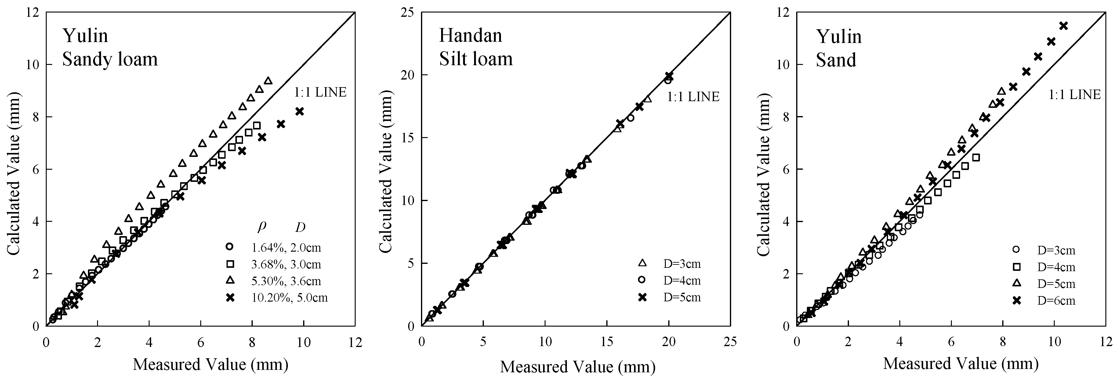
Three published data sets were then next selected for a more thorough evaluation of the simplified model established in this study. The first data set was obtained from Li [21], and the experimental soil was sandy loam with dry bulk density of 1.30 g·cm⁻³, which was taken from the Yulin region, located in the North Loess Plateau, China. The cumulative infiltration was analyzed with four different combinations of the ρ and D values. The D of the experiments was 2–5 cm. The second data set came from Hu [38], whose experimental soil was silt loam with bulk density of 1.35 g·cm⁻³, selected from Handan City, located in the North China Plain. The D of the experiments was 3–5 cm and the spacing between holes was 17.5 cm. The third data set obtained by Wu [18] with sand as the experimental soil and bulk density of 1.52 g·cm⁻³, which taken from the Yulin region. The film hole diameters in the experiment were 3–6 cm, and the spacing between holes was 12 cm. The details from these experiments have been provided in their respective publications.

A comparison between the calculated and measured values of the cumulative infiltration of a single film hole within the controlling area under different D and ρ values is illustrated in Figure 12. Equations (25)–(27) are the simplified model equations for each soil type motioned above; the MAE, RMSE, PBIAS, and NS values for measured and calculated cases are presented in

Table 5. Correlation between measured and calculated values of cumulative infiltration.

Soil	MAE (mm)	RMSE (mm)	PBIAS (%)	NS
Loam from Wugong	0.190	0.190	−2.131	0.995
Silt Loam from Weihe Bench	0.391	0.552	−1.082	0.997
Loam from Luochuan	2.299	2.722	−1.756	0.989
Sandy Loam from Ansai	0.508	0.830	−1.375	0.985
Sandy Loam from Yulin	0.431	0.566	1.479	0.999
Silt Loam from Handan	0.141	0.177	−1.569	0.982
Sand from Yulin	0.390	0.466	−1.170	0.998

. The MAE, RMSE, and PBIAS values ranged from 0.141 to 2.299 mm, 0.177 to 2.722 mm, and −2.131% to 1.479%, respectively; meanwhile, the NS values were very close to 1.0. Notably, all results were in good agreement, indicating that the model can effectively describe the characteristics of film hole infiltration.

$$I=62.64({\rho }^{1.131}/D^{0.698})t^{0.7415-\rho }$$

(25)

$$I=51.05({\rho }^{1.131}/D^{0.698})t^{0.9217-\rho }$$

(26)

$$I=480.53({\rho }^{1.131}/D^{0.698})t^{0.9245-\rho }$$

(27)

4. Conclusions

Film hole infiltration is a low-cost and high-efficiency irrigation method that is widely used in China. In this study, the SWMS-2D-simulated wetting patterns and cumulative infiltration observed for film hole irrigation were in good agreement with experimental observations for silt loam and sandy loam at different soil bulk densities. Therefore, the SWMS-2D model is suitable for simulating film hole irrigation. In addition, the initial SWC and irrigation depth had little effect on cumulative infiltration during film hole irrigation, whereas the D and ρ significantly affected the cumulative infiltration. Furthermore, the observed cumulative infiltration increased with ρ, but it decreased with increased D with the same ρ. Finally, we proposed a simplified model for film hole irrigation, and this model has extensive applicability. In conclusion, cumulative infiltration can be adequately described with D and ρ for a soil with certain texture and bulk density.

References

- Matti, K.; Ward, P.J.; Moel, H.D.; Varis, O. Is physical water scarcity a new phenomenon? Global assessment of water shortage over the last two millennia. Environ. Res. Lett. 2010, 5. [Google Scholar] [CrossRef] [Green Version]
- Wallace, J.S. Increasing agricultural water use efficiency to meet future food production. Agric. Ecosyst. Environ. 2001, 82, 105–119. [Google Scholar] [CrossRef]
- Swatuk, L.; Mcmorris, M.; Leung, C.; Zu, Y. Seeing “invisible water”: Challenging conceptions of water for agriculture, food and human security. Can. J. Dev. Stud. 2015, 36, 24–37. [Google Scholar] [CrossRef]
- Deng, X.P.; Shan, L.; Zhang, H.; Turner, N.C. Improving agricultural water use efficiency in arid and semiarid areas of China. Agric. Water Manag. 2006, 80, 23–40. [Google Scholar] [CrossRef]
- Li, X.Y.; Gong, J.D.; Wei, X.H. In-situ rainwater harvesting and gravel mulch combination for corn production in the dry semi-arid region of China. J. Arid Environ. 2000, 46, 371–382. [Google Scholar] [CrossRef]
- Camp, C.R. Subsurface drip irrigation: A review. Trans. ASAE 1998, 41, 1353–1367. [Google Scholar] [CrossRef]
- Tarara, J.M. Microclimate modification with plastic mulch. Hortscience 2000, 35, 169–180. [Google Scholar]
- McKenzie, C.; Duncan, L.W. Landscape fabric as a physical barrier to neonate diaprepes abbreviatus (Coleoptera: Curculionidae). FL Entomol. 2001, 84, 721–722. [Google Scholar] [CrossRef]
- Chalker-Scott, L. Impact of mulches on landscape plants and the Environment—A review. J. Environ. Hort. 2007, 25, 239–249. [Google Scholar]
- Espí, E.; Salmerón, A.; Fontecha, A.; García, Y.; Real, A.I. Plastic films for agricultural applications. J. Plast. Film Sheet 2006, 22, 85–102. [Google Scholar] [CrossRef]
- Lamont, W.J. Plastic mulches for the production of vegetable crops. Horttechnology 1993, 3, 35–39. [Google Scholar]
- Scarasciamugnozza, G.; Sica, C.; Russo, G. Plastic materials in European agriculture: Actual use and perspectives. J. Agric. Eng. 2011, 42, 15–28. [Google Scholar] [CrossRef]
- Steinmetz, Z.; Wollmann, C.; Schaefer, M.; Buchmann, C.; David, J.; Tröger, J.; Muñoz, K.; Frör, O.; Schaumann, G.E. Plastic mulching in agriculture. Trading short-term agronomic benefits for long-term soil degradation? Sci. Total Environ. 2016, 550, 690–705. [Google Scholar] [CrossRef] [PubMed]
- Kader, M.A.; Senge, M.; Mojid, M.A.; Ito, K. Recent advances in mulching materials and methods for modifying soil environment. Soil Till. Res. 2017, 168, 155–166. [Google Scholar] [CrossRef]
- National Bureau of Statistics of China. China Statistical Year Book 2014; National Bureau of Statistics of China: Beijing, China, 2014.
- Xu, S. Fim hole irrigation technology. Xinjiang Water Res. 1994, 83, 22–26. (In Chinese) [Google Scholar]
- Saeed, M.; Mahmood, S. Application of film hole irrigation on borders for water saving and sunflower production. Arab J. Sci. Eng. 2013, 38, 1347–1358. [Google Scholar] [CrossRef]
- Wu, J.; Fei, L.; Wang, W. Study on the infiltration characteristics of single filmed hole and its mathematical model under filmed hole irrigation. Adv. Water Sci. 2001, 9, 307–311. (In Chinese) [Google Scholar]
- Li, Y.; Tian, J. Research advances irrigating technique of film hole irrigation. J. Ningxia Agric. Coll. 2003, 24, 96–100. (In Chinese) [Google Scholar]
- Bautista, E.; Clemmens, A.J.; Strelkoff, T.S.; Schlegel, J. Modern analysis of surface irrigation systems with WinSRFR. Agric. Water Manag. 2009, 96, 1146–1154. [Google Scholar] [CrossRef]
- Li, F.; Zhang, X.; Fei, L. Experimental study on influential factors in film hole bilateral interference infiltration. J. Irrig. Drain. 2002, 22, 44–48. (In Chinese) [Google Scholar]
- Dong, Y.; Wang, B.; Jia, L.; Fei, L. Effects of different irrigation treatments on maize water consumption, growth and yield under film hole irrigation. Appl. Mech. Mater. 2014, 501–504, 1986–1992. [Google Scholar] [CrossRef]
- Šimůnek, J.; Huang, K.; Genuchten, M.T.V. The SWMS-2D Code for Simulating Water Flow and Solute Transport in Two-Dimensional Variably-Saturated Media; Version 1.0; US Salinity Laboratory, US Department of Agriculture, Agricultural Research Service: Riverside, CA, USA, 1995.
- Skaggs, T.H.; Trout, T.J.; Simunek, J.; Shouse, P.J. Comparison of HYDRUS-2D simulations of drip irrigation with experimental observations. J. Irrig. Drain. Eng. 2014, 130, 304–310. [Google Scholar] [CrossRef]
- Zhou, Q.Y.; Kang, S.Z.; Zhang, L. Comparison of APRI and Hydrus-2D models to simulate soil water dynamics in a vineyard under alternate partial root zone drip irrigation. Plant Soil 2007, 291, 211–223. [Google Scholar] [CrossRef]
- Lazarovitch, N.; Poulton, M.; Furman, A.; Warrick, A.W. Water distribution under trickle irrigation predicted using artificial neural networks. J. Eng. Math. 2009, 64, 207–218. [Google Scholar] [CrossRef]
- Mguidiche, A.; Provenzano, G.; Douh, B.; Khila, S.; Rallo, G.; Boujelben, A. Assessing hydrus-2D to simulate soil water content (SWC) and salt accumulation under an SDI system: Application to a potato crop in a semi-arid area of Central Tunisia. Irrig. Drain. 2015, 64, 263–274. [Google Scholar] [CrossRef]
- Hou, L.; Zhou, Y.; Bao, H.; Wenninger, J. Simulation of maize (Zea mays L.) water use with the HYDRUS-1D model in the semi-arid Hailiutu River catchment, Northwest China. Hydrol. Sci. J. 2016, 62, 1–11. [Google Scholar] [CrossRef]
- Kandelous, M.M.; Šimůnek, J. Numerical simulations of water movement in a subsurface drip irrigation system under field and laboratory conditions using HYDRUS-2D. Agric. Water Manag. 2010, 97, 1070–1076. [Google Scholar] [CrossRef]
- Jiang, L. Technique element of film hole infiltration on cotton. China Rural Water Hydropower 1995, 5, 3–6. (In Chinese) [Google Scholar]
- Zhang, G.; Zhu, L. Study on irrigating technique of film hole irrigation in Weibei dry plateau. Res. Soil Water Conserv. 1999, 6, 60–63. (In Chinese) [Google Scholar]
- Xing, X.; Kang, D.; Ma, X. Differences in loam water retention and shrinkage behavior: Effects of various types and concentrations of salt ions. Soil Till. Res. 2017, 167, 61–72. [Google Scholar] [CrossRef]
- Yao, W.W.; Ma, X.Y.; Li, J.; Parkes, M. Simulation of point source wetting pattern of subsurface drip irrigation. Irrig. Sci. 2011, 29, 331–339. [Google Scholar] [CrossRef]
- Maulem, Y. A new model for predicting the hydraulic conductivity of unsaturated porous media. Water Resour. Res. 1976, 12, 513–522. [Google Scholar] [CrossRef]
- Van Genuchten, M.T.; Leij, F.J.; Yates, S.R. The RETC Code for Quantifying the Hydraulic Functions of Unsaturated Soils; Research Report No. EPA/600/2-91/065; US Salinity Laboratory, US Department of Agriculture, Agricultural Research Service: Riverside, CA, USA, 1991. Available online: http://www.pc-progress.com/documents/programs/retc.pdf (accessed on 1 December 1991).
- Moriasi, D.; Arnold, J.; Van Liew, M.W.; Veith, T.L. Model evaluation guidelines for systematic quantification of accuracy in watershed simulations. Trans. ASABE 2007, 50, 885–900. [Google Scholar] [CrossRef]
- Ma, X.; Fan, Y.; Wang, S.; Sun, X.; Wang, B. Simplified Infiltration Model of Film Hole Irrigation and Its Validation. Trans. Chin. Soc. Agric. Mach. 2009, 40, 67–73. (In Chinese) [Google Scholar]
- Hu, H. Soil Water and Nitrogen Transport Characteristic Experiment and Numerical Simulation of Film Hole Irrigation under Facilities. Ph.D. Dissertation, Wuhan University, Wuhan, China, 2010. (In Chinese). [Google Scholar]
Figure 1.
Simplified experimental setup (h0 represents irrigation depth).
Figure 2.
Simplified graph of film hole irrigation model ((a) represents the three-dimensional axisymmetric domain; (b) represents the wetting pattern during the infiltration process).
Figure 3.
Measured (dots) and fitted (line) water retention and diffusivity curves of silt loam and sandy loam using the van Genuchten–Mualem Model.
Figure 4.
Comparison of simulated and measured values of soil wetting patterns (Measured data are represented by black dots, whereas simulated values are shown using water content as contour lines).
Figure 5.
Comparison of simulated and measured values of cumulative infiltration under different treatments (cumulative infiltration represents the irrigation volume of the controlling area of a single hole in the experimental setup (see Figure 1); measured values are represented by dots, whereas simulated values are represented by lines).
Figure 6.
Effect of initial SWC on film hole infiltration: (a) silt loam γd = 1.30 g·cm−3; (b) sandy Loam γd = 1.35 g·cm−3; and (c) loamy sand (the percentage is the percentage of field capacity).
Figure 7.
Infiltration pattern curves under different irrigated water depths: (a) silt loam, γd = 1.30 g·cm−3; (b) sandy loam, γd = 1.35 g·cm−3; and (c) loamy sand.
Figure 8.
Effect of layered soil depth on film hole infiltration. (a) Experimental soils: 1–4 sandy loam (γd = 1.35 g·cm−3) + silt loam (γd = 1.30 g·cm−3); 5–8 silt loam (γd = 1.40 g·cm−3) + sandy loam (γd = 1.45 g·cm−3); (b) The soils selected from RETC software: 1–4 loamy sand + loam, 5–8 loam + loamy sand; (c) Double bulk densities: 1–4 silt loam, 1.40 g·cm−3 + 1.30 g·cm−3; 5–8 sandy loam, 1.35 g·cm−3 + 1.45 g·cm−3. For Nos. 1–8: 1 and 5—upper depth 15 cm; 2 and 6—upper depth 20 cm; 3 and 7—upper depth 30 cm; 4 and 8—homogeneity.
Figure 9.
Infiltration pattern curve under different film hole spacing: (a1,a2) silt loam, γd = 1.30 g·cm−3; (b1,b2) sandy loam, γd = 1.45 g·cm−3; (c1,c2) loam; and (d1,d2) sand. In the legend, the percentage values are equal to ρ, and the following values are equal to D.
Figure 10.
Comparison of simulated and estimated k and α. Nos. 1–13 indicate 13 types of tested soil form experiments performed using RETC software: 1 = silt loam (1.30 g·cm−3); 2 = silt loam (1.30 g·cm−3); 3 = sandy loam (1.35 g·cm−3); 4 = sandy loam (1.45 g·cm−3); 5 = loam; 6 = sand; 7 = sandy loam; 8 = loamy sand; 9 = silt; 10 = silt loam; 11 = sandy clay loam; 12 = clay loam; and 13 = silt clay loam.
Figure 11.
Comparison of four soil types between calculated values and measured values of cumulative infiltration.
Figure 12.
Comparison of three infiltration models (cited from published studies) between calculated and measured values of cumulative infiltration.