Simulation of Typhoon-Induced Storm Tides and Wind Waves for the Northeastern Coast of Taiwan Using a Tide–Surge–Wave Coupled Model


1
National Science and Technology Center for Disaster Reduction, New Taipei City 23143, Taiwan
2
Department of Hydraulic and Ocean Engineering, National Cheng Kung University, Tainan City 70101, Taiwan
*
Author to whom correspondence should be addressed.
Water 2017, 9(7), 549; https://doi.org/10.3390/w9070549
Submission received: 13 June 2017
/
Revised: 17 July 2017
/
Accepted: 19 July 2017
/
Published: 21 July 2017
Abstract
:The storm tide is a combination of the astronomical tide and storm surge, which is the actual sea water level leading to flooding in low-lying coastal areas. A full coupled modeling system (Semi-implicit Eulerian-Lagrangian Finite-Element model coupled with Wind Wave Model II, SELFE-WWM-II) for simulating the interaction of tide, surge and waves based on an unstructured grid is applied to simulate the storm tide and wind waves for the northeastern coast of Taiwan. The coupled model was driven by the astronomical tide and consisted of main eight tidal constituents and the meteorological forcings (air pressure and wind stress) of typhoons. SELFE computes the depth-averaged current and water surface elevation passed to WWM-II, while WWM-II passes the radiation stress to SELFE by solving the wave action equation. Hindcasts of wind waves and storm tides for five typhoon events were developed to validate the coupled model. The detailed comparisons generally show good agreement between the simulations and measurements. The contributions of surge induced by wave and meteorological forcings to the storm tide were investigated for Typhoon Soudelor (2015) at three tide gauge stations. The results reveal that the surge contributed by wave radiation stress was 0.55 m at Suao Port due to the giant offshore wind wave (exceeding 16.0 m) caused by Typhoon Soudelor (2015) and the steep sea-bottom slope. The air pressure resulted in a 0.6 m surge at Hualien Port because of an inverted barometer effect. The wind stress effect was only slightly significant at Keelung Port, contributing 0.22 m to the storm tide. We conclude that wind waves should not be neglected when modeling typhoon-induced storm tides, especially in regions with steep sea-bottom slopes. In addition, accurate tidal and meteorological forces are also required for storm tide modeling.
1. Introduction
Typhoon-induced storm surge and wind waves are major forces that pose a potential hazard in the form of coastal inundation and to shipping routes. Storm surge is classified as long gravity waves, whereas wind wave are short-period waves. Only long gravity waves can ascend to land, causing inundation that leads to severe loss of life and substantial damage to infrastructure in low-lying areas near the coast. Although short-period wind waves could be dangerous over the ocean, they would break at shallow waters and cannot climb land. Storm tide is the actual level of the water in the sea and adjacent tidal waterways during a typhoon event. The storm tide level results from the additive combination of the normal astronomical tide and the increase in water level due to the storm surge. The total surge depends on the interaction of wave forcing, wind stress, inverted barometer effects, tidal stage and bathymetry in the path of the typhoon [1,2,3,4,5,6,7]. The wave-induced radiation stress was usually neglected in early storm surge modeling [8,9,10,11,12,13,14,15,16]. The contributions of wind waves to the momentum equation were replaced by adding an additional drag coefficient to the wind stress equation. Although this simple method is convenient in storm surge modeling, the momentum transfer rate from wave breaking is highly dependent on the slope and depth of the sea-bottom [17]. Fully coupled wave–current models based on structured or unstructured grids have been recently developed for storm tide modeling despite the high computational cost [6,7,18,19,20,21,22].
To better understand the wave effects on storm tide modeling, the tide–surge–wave coupled modeling system based on unstructured grids was implemented for the Taiwan Waters in this study, and fully coupled simulations were conducted for storm tides and wind waves using an unstructured-grid finite-element model. This paper is organized as follows. The study site and unstructured grid system for the numerical model are described in Section 2. A brief outline of models used in the present study is given in Section 3. Section 4 describes the model validation for typhoon-induced storm tides and waves. In Section 5, numerical experiments were conducted to investigate the contributions of wave-, wind stress- and air pressure-induced surge to storm tides. The conclusions are summarized in the last section.
2. Description of Study Area
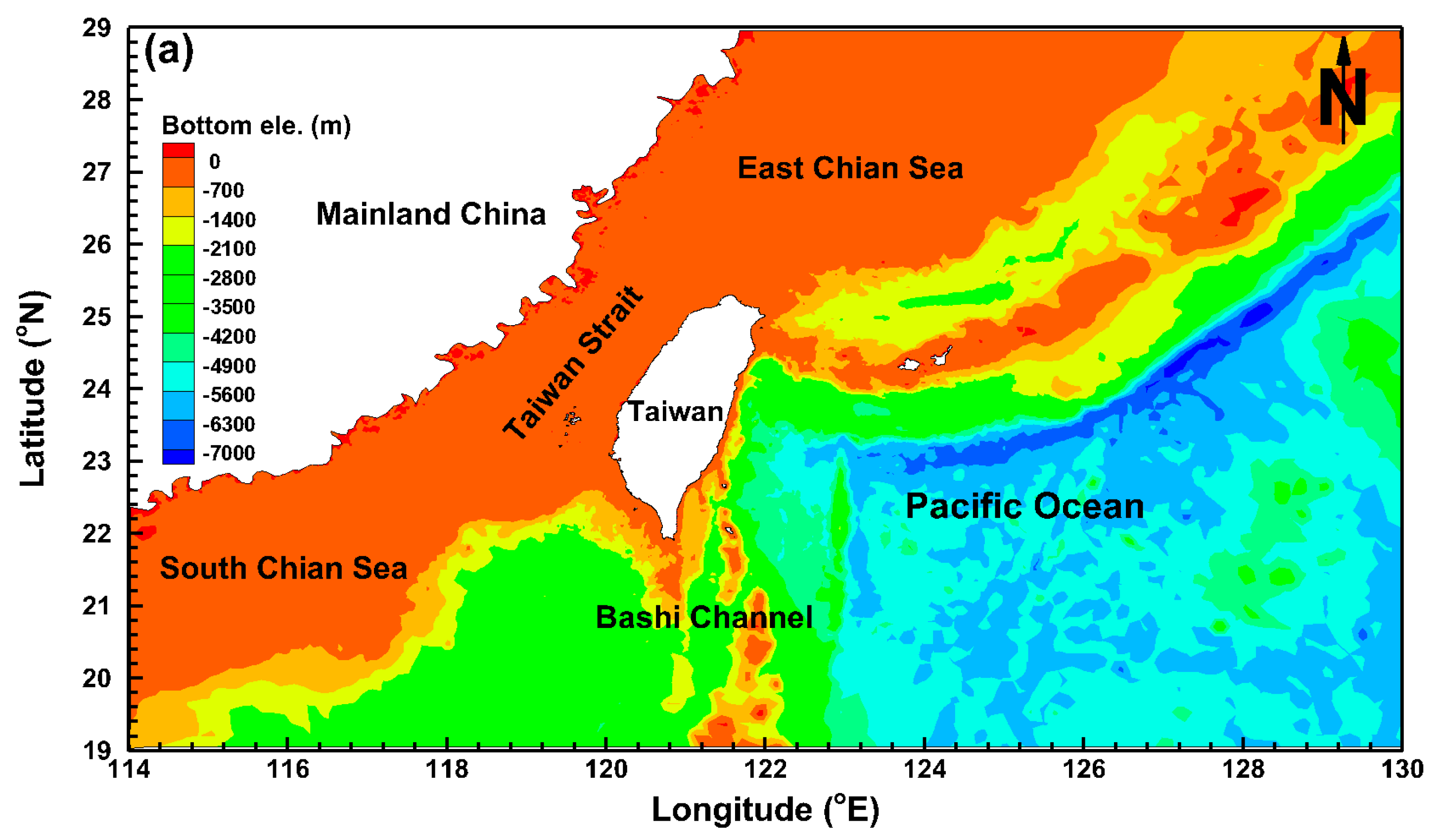
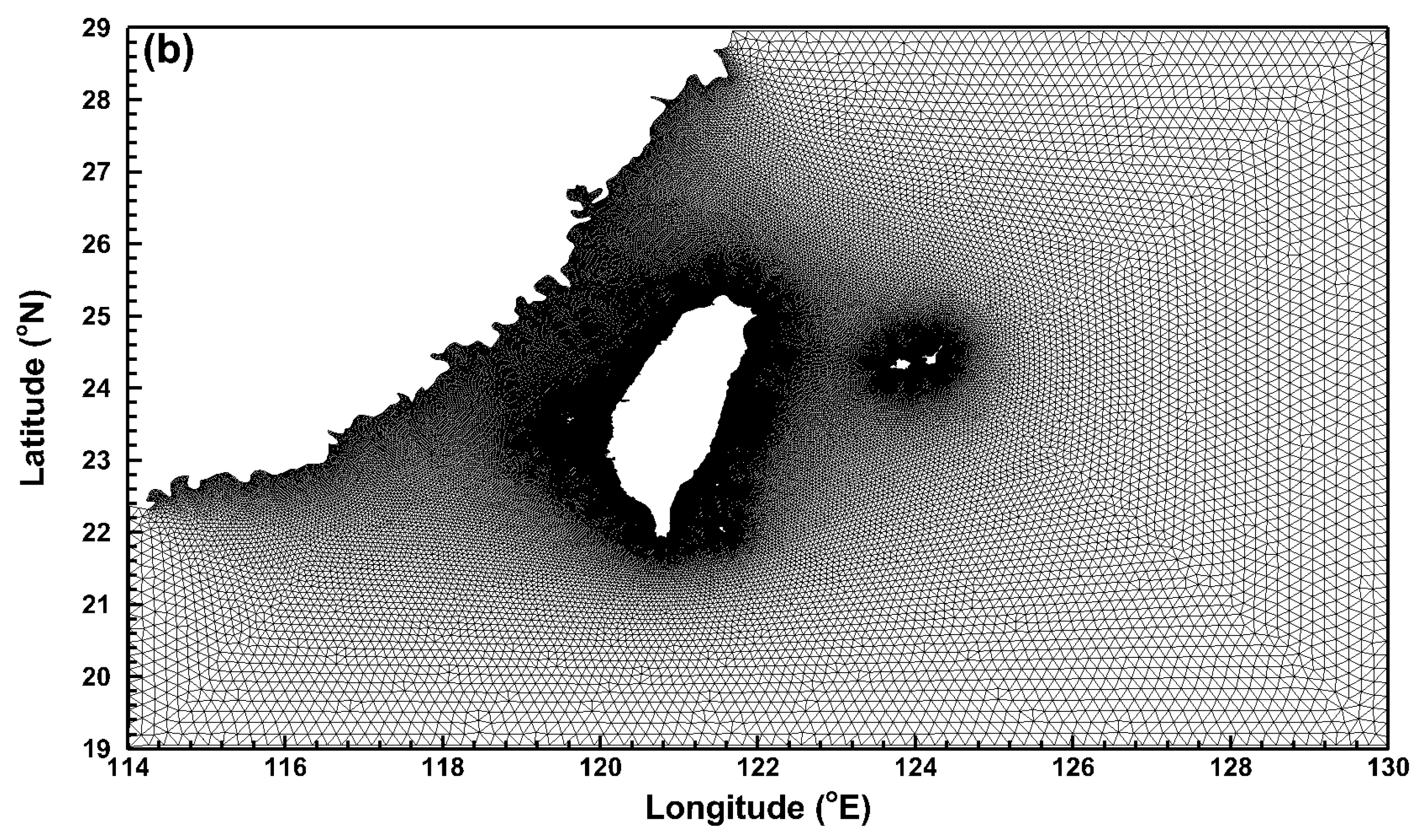
The computational domain in the present study covers the region within a longitude of 114° to 130° E and latitude of 19° to 29° N. This area is composed of the western Pacific Ocean, the Taiwan Strait, the South China Sea and the East China Sea, which are located in the east, the west, the south and the north of Taiwan, respectively (Figure 1a). The bathymetric data used in the present study were obtained from coastal digital elevation models (DEMs) and ETOPO1 [23], a global relief model. ETOPO1 integrates land topography and the ocean bathymetry of Earth’s surface with a 1-arc-minute resolution. It is quite clear in Figure 1a that the sea-bottom elevations along the eastern coast of Taiwan are very steep. The bottom elevations vary rapidly from tens of meters at the shoreline to several thousand meters at 10 km off the coast. With respect to the north coast, the slopes of the sea-bottom are relatively flatter. A total of 278,630 non-overlapping unstructured triangular cells and 142,041 nodes were used in the horizontal to fit the complex shoreline of Taiwan and its adjacent small islands. The resolutions of the mesh range from 30 km to 300 m. The fine meshes are along the coastline of Taiwan and small offshore islands, while the coarse meshes are along the open ocean boundaries (Figure 1b).
3. Methodology
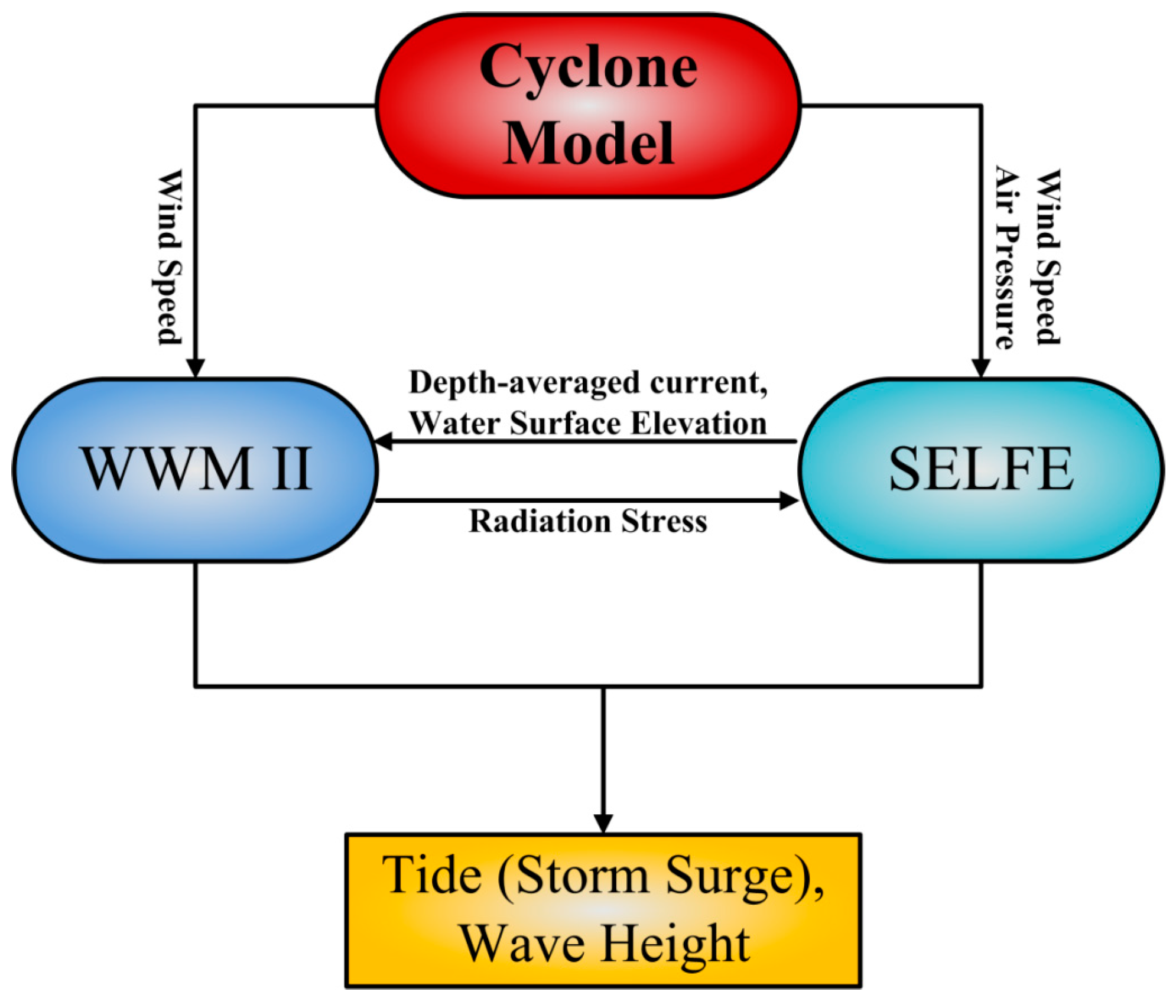
The effects of the wave forcing and meteorological forcing induced by typhoons on storm tide modeling are taken into account using the coupled modeling system for wind waves, tide and storm surge. The numerical tide–surge–wave modeling system used in the present study consists of a hydrodynamic model (Semi-implicit Eulerian-Lagrangian Finite-Element model, SELFE [24]) and a third-generation spectral wind wave model (Wind Wave Model II, WWM-II [25]). The same computational domain and unstructured-grid system are shared in the coupled model SELFE-WWM-II [26], which avoids the need for data interpolation between the two models and ensures parallel efficiency. SELFE computes the depth-averaged current and water surface elevation passed to WWM-II, while WWM-II passes the radiation stress to SELFE by solving the wave action equation. Figure 2 shows a schematic diagram of the coupled modeling system. More details about the processes of model coupling and model validation with analytical solutions can be found in [26].
3.1. The Hydrodynamic Model
The hydrodynamic model, SELFE, coupled with WWM-II, is used to compute tides and surges. SELFE is a semi-implicit Eulerian–Lagrangian finite-element model that has been widely used for the simulation of tsunami propagation [27], water quality and ecosystem dynamics [28,29], oil spill dynamics [30], generating inundation maps [31,32] and modeling inundation induced by extreme river flows, typhoons and hurricanes [33,34]. The SELFE model used in the present study is a two-dimensional vertically integrated version with a barotropic mode (SELFE-2DH). The governing equations in two-dimensional form are given as:
where is the free-surface elevation; , is the bathymetric depth; and are the horizontal velocity in the direction, respectively; is the Coriolis factor; g is the acceleration due to gravity; is the earth’s tidal potential; is the effective earth elasticity factor; is the reference density of water; and is the atmospheric pressure at the free surface. and are the wind stress in the direction, which can be expressed as:
where is the wind drag coefficient; is the air density; and are the wind speed in components. Although is often modeled as an increasing function of wind velocity, Powell et al. [35] suggested that should be limited at high wind speed. The formula for calculating the in SELFE-2HD is as:
where is the wind speed at 10 m above the sea surface.
and are the wave-induced stresses in the direction, which can be computed following [36]:
where , and are the wave radiation stresses and are represented according to [37]:
where is the wave action, is the wave relative angular frequency, is the wave direction, and and are the wave group velocity and wave phase velocity, respectively.
and are the bottom shear stress in the direction and are computed by following formula:
where is the bottom drag coefficient, and can be parameter
where is the Manning coefficient and will be determined through the model validation. A time step of 120 s was used for the hydrodynamic model in simulations with no signs of numerical instability for the present model grid system. The time step of WWM-II is 600 s, i.e., SELFE and WWM-II exchange information every five hydrodynamic time steps. Chen et al. [38] used the coupled ADCRIC+SWAN model to predict the storm surges and wind waves in Mobile Bay, Alabama. They exchanged the hydrodynamic model information with the wind wave model every 30 min and suggested that model results are insensitive to increases in the exchange frequency.
3.2. The Spectral Wind Wave Model
The governing equation for the third-generation spectral wind wave model, WWM-II, is the wave action equation, given as:
where is the wave action, and are the wave group velocity in the direction, and are the horizontal velocity in the direction, is the wave relative angular frequency, is the wave direction, and are the propagation velocity in space, and is the sum of the source terms for wave variance. The maximum wave direction in WWM-II is 360°, and this measure is discretized into 36 bins. The low- and high-frequency limits of the discrete wave period are 0.03 and 1.0 Hz, respectively, and are divided into 36 bins. The bottom friction is set equal to 0.067 based on the formulation of JONSWAP [39]. The wave breaking in shallow water area is computed in WWM-II using the method presented by [40] with a constant wave breaking coefficient of 0.78.
3.3. Global Model for the Prediction of Ocean Tides
For many practical applications of modeling in coastal environments, accurate predictions of tidal currents and elevations are always indispensable. Due to the necessity of simulating the interaction between astronomical tide and storm surge, the driving forces at the open boundaries of the tide–surge model are tidal elevations. In the present study, a global ocean tidal prediction model, TPXO, developed by Oregon State University, was adopted to extract the tidal harmonic constants and then specified at the open boundaries of SELFE-2HD for simulating tidal propagation. TPXO uses inverse theory and measured data assimilated from tide gauges and the TOPEX/Poseidon satellite. This model finds an optimum balance between observations and hydrodynamics. The extracted tidal harmonic constants provided complex amplitudes of the earth-relative sea-surface elevation for eight primary (M2, S2, N2, K2, K1, O1, P1 and Q1) tidal constituents. The detailed methodologies used to compute the tides in TPXO can be found in [41,42].
3.4. Parametric Cyclone Model
The meteorological boundary conditions for storm surge calculation consist of the wind speed and atmospheric pressure of typhoons. A common way to generate wind and air pressure fields for typhoons is to reconstruct them using the analytical parametric cyclone model. Over the years, many parametric cyclone models have been developed to provide meteorological information for storm surge modeling [43,44,45,46,47,48]. Jakobsen and Madsen [49] investigated and compared parametric cyclone models based on cyclone position, central pressure, maximum wind speed and radius to maximum wind speed. They found that the analytical models provide very similar air pressure and tangential wind speed distributions for a cyclone. Therefore, a parametric cyclone model presented by Holland [45] was employed:
where is the air pressure; is the ambient pressure; the central air pressure of the typhoon; is the radius to the maximum wind speed; is the radial distance from the typhoon center; is the wind speed; is the air density; is the Coriolis factor; and is a parameter that characterizes the scale of the typhoon. The wind field was modified from gradient height to 10 m above sea surface with a wind-reducing coefficient of 0.85 following [50]. The formula of presented by Hubbert et al. [51] was adopted. With regard to the estimation of , the formula used to simulate the storm surge in the northwest Pacific Ocean [52] was adopted in this study:
where ; , and were set to be 5.0377, −0.0232 and 0.4502, respectively [52].
Holland model is an axisymmetric model, the asymmetric structure of a typhoon cannot be represented by the model. Highly asymmetric structures in a landfalling typhoon often lead to large errors in storm surge forecasting. To overcome this limitation, Georgiou [53] introduced a hurricane translation speed () to Holland model and was used in the present study:
is the total wind speed; is the typhoon translation speed; are the wind speed in components; is the angle from the direction of the hurricane movement; is the azimuthal angle with respect to the typhoon’s eye; and is the inflow angle at the surface. Although the local wind and surge estimates are less sensitive to inflow angle [50], the inflow angle was considered in the present study, and can be described as a function of [54]:
Table 1 lists the parameters used in SELFE-WWM-II and parametric cyclone model.
3.5. Indicators of Model Performance
Three criteria are adopted to assess the model performance for water level simulation, including the mean absolute error (MAE), the root mean square error (RMSE), and percent bias (PBIAS) [55]. The optimal value of PBIAS is 0, with low-magnitude values indicating accurate model simulations. Positive values of PBIAS indicate that the model was overestimating while negative values indicate that the model was underestimating [56]. The equations for these three criteria are shown as follows:
is the simulations and is the measurements.
4. Model Validation
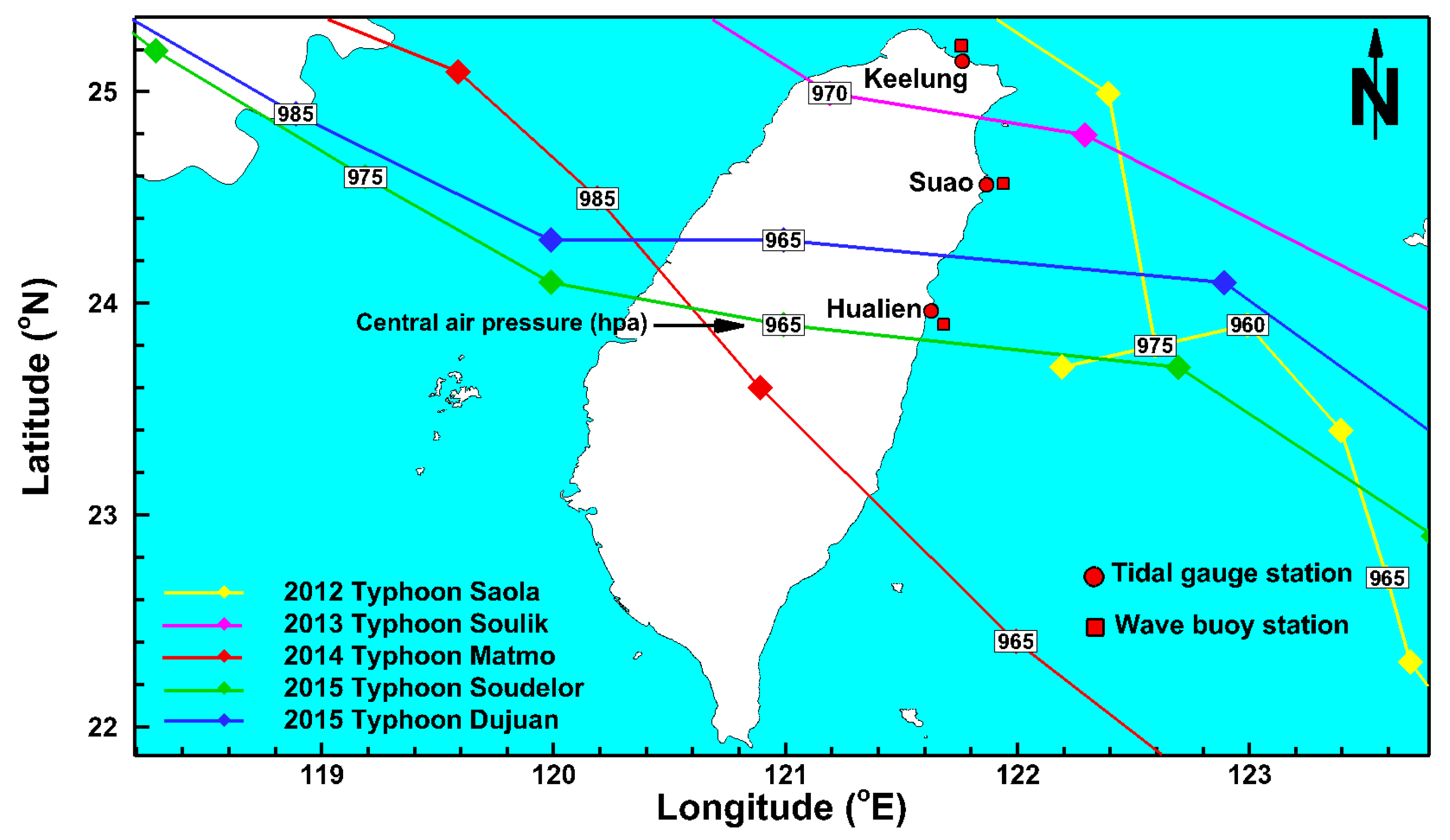
The hindcasts of wave height and storm tide induced by five typhoon events, including Typhoon Saola (2012), Typhoon Soulik (2013), Typhoon Matmo (2014), Typhoon Soudelor (2015) and Typhoon Dujuan (2015), were conducted to validate the coupled model. The paths of these five typhoons were crossed or passed Taiwan from the east to the west or from the southeast to the northwest. Besides, the 10 min average wind speed near the typhoon center were in the range of 38 m/s to 51 m/s, and were classified as the moderate to the severe typhoon (according to the categories of Central Weather Bureau in Taiwan). Therefore, the surges induced by these five typhoons would be significant along the northeastern of Taiwan.
The tracks of these five typhoons and their corresponding central air pressures are shown in Figure 3. Three wave buoys (Keelung buoy, Suao buoy and Hualien buoy) and three tide gauge stations (Keelung Port, Suao Fish Port and Hualien Port) located along the northeastern coast of Taiwan were selected to compare wave heights and sea water levels between the simulations and observations. Figure 3 also illustrates the locations of wave buoys and tide gauge stations. The historical data used to construct the wind and air pressure fields for the five typhoon events were obtained from The Regional Specialized Meteorological Center (RSMC) Tokyo-Typhoon Center Best Track database. Hourly data for wave height and sea water level measured at three wave buoys and three tide gauge stations were provided by the Harbor and Marine Technology Center and the Central Weather Bureau in Taiwan.
4.1. Validation of Storm Tide
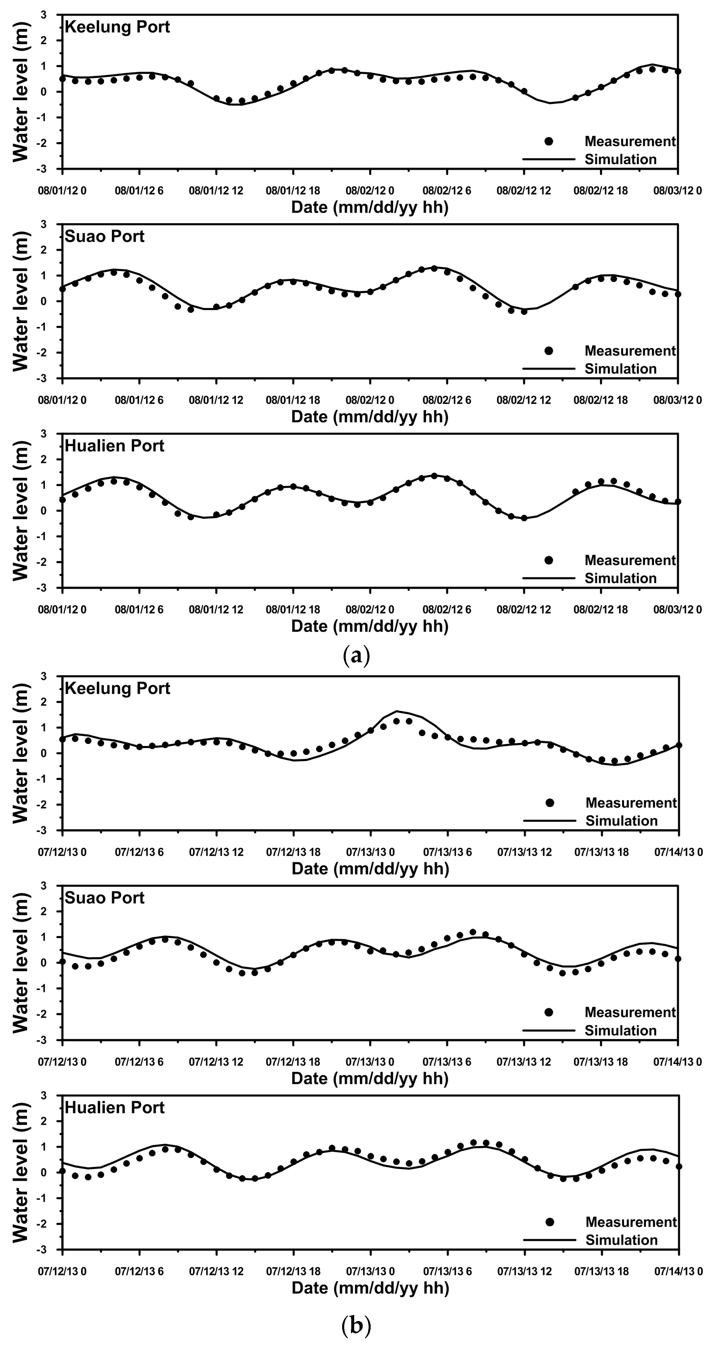
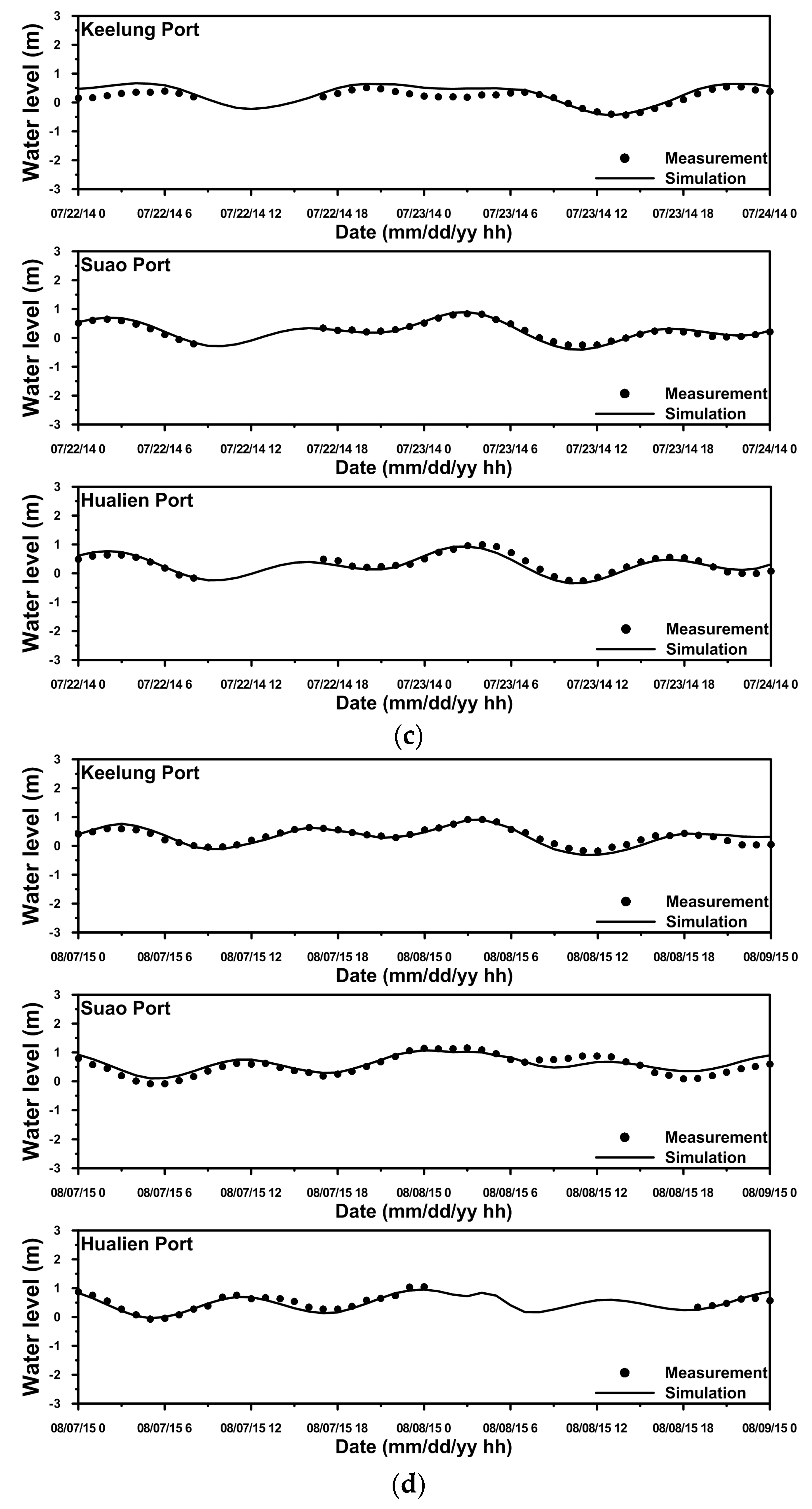
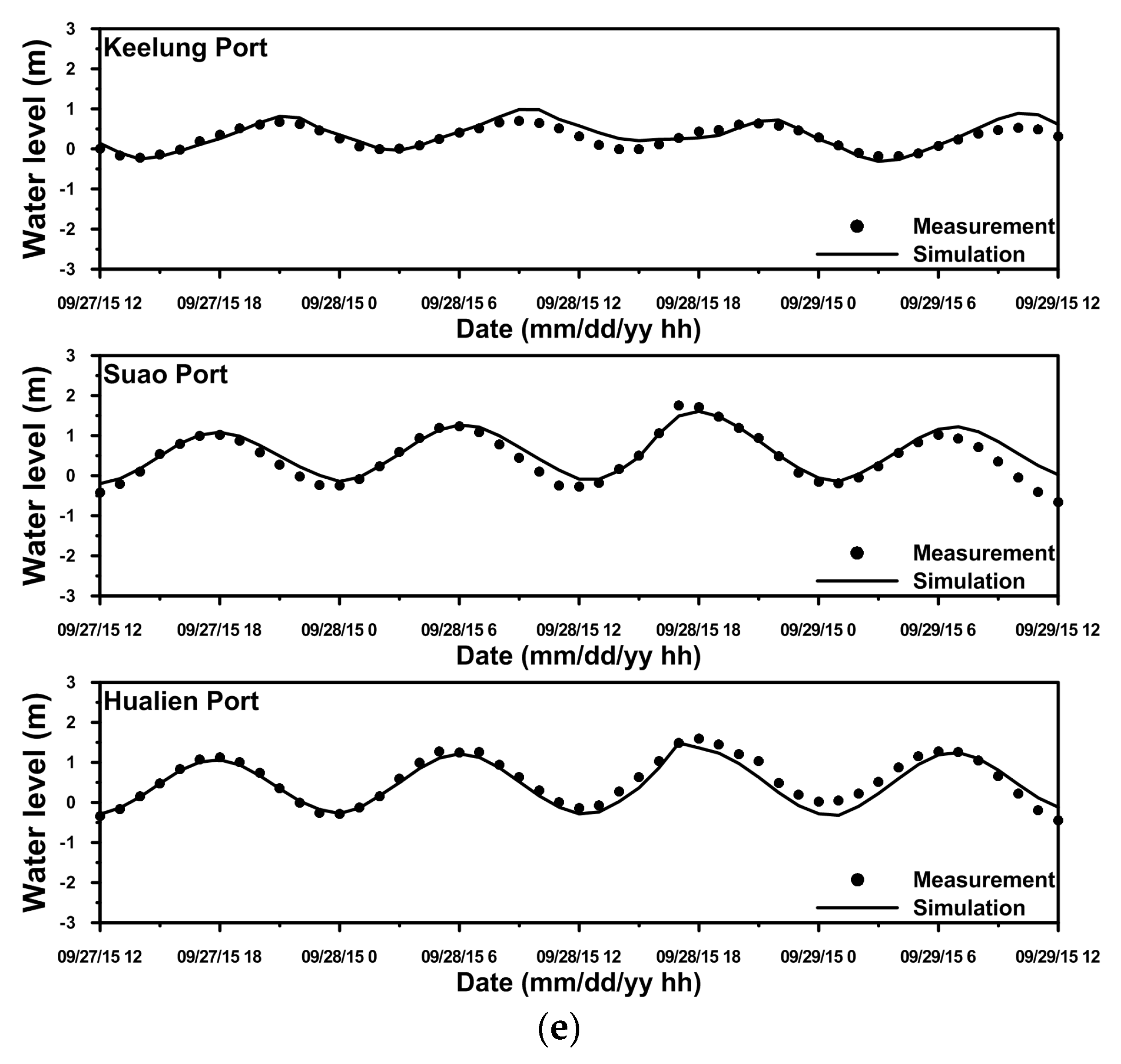
Figure 4 presents the comparisons of the modeled and observed water levels at Keelung Port, Suao Fish Port and Hualien Port for the five typhoon events. Although the water level hydrographs show that the simulations have good agreements with the observations in both astronomical tides and storm tides, the model results sometimes underestimate or overestimate the water level. These discrepancies may be due to the inaccuracy of the wind field and air pressure field created by the parametric cyclone model. The parametric cyclone model has difficulty representing the accurate structure of typhoons at certain locations and is not expected to reproduce the wind conditions far away from the center [54]. Feng et al. [57] also suffered from a similar problem when Jelesnianski’s circular hurricane model was employed to simulate storm surge at Tianjin in China. The statistical errors for the differences between the simulated and observed water levels at three tidal gauge stations can be found in Table 2. The maximum MAE is 0.11 m for Keelung Port, while the minimum MAE is 0.09 m for Hualien Port. The RMSE is 0.12 m for Keelung Port and Suao Port and 0.09 m for Hualien Port. PBIAS is below 10% for Keelung Port and Suao Port and approximately −5% for Hualien Port.
4.2. Validation of Wave Height and Wave Period
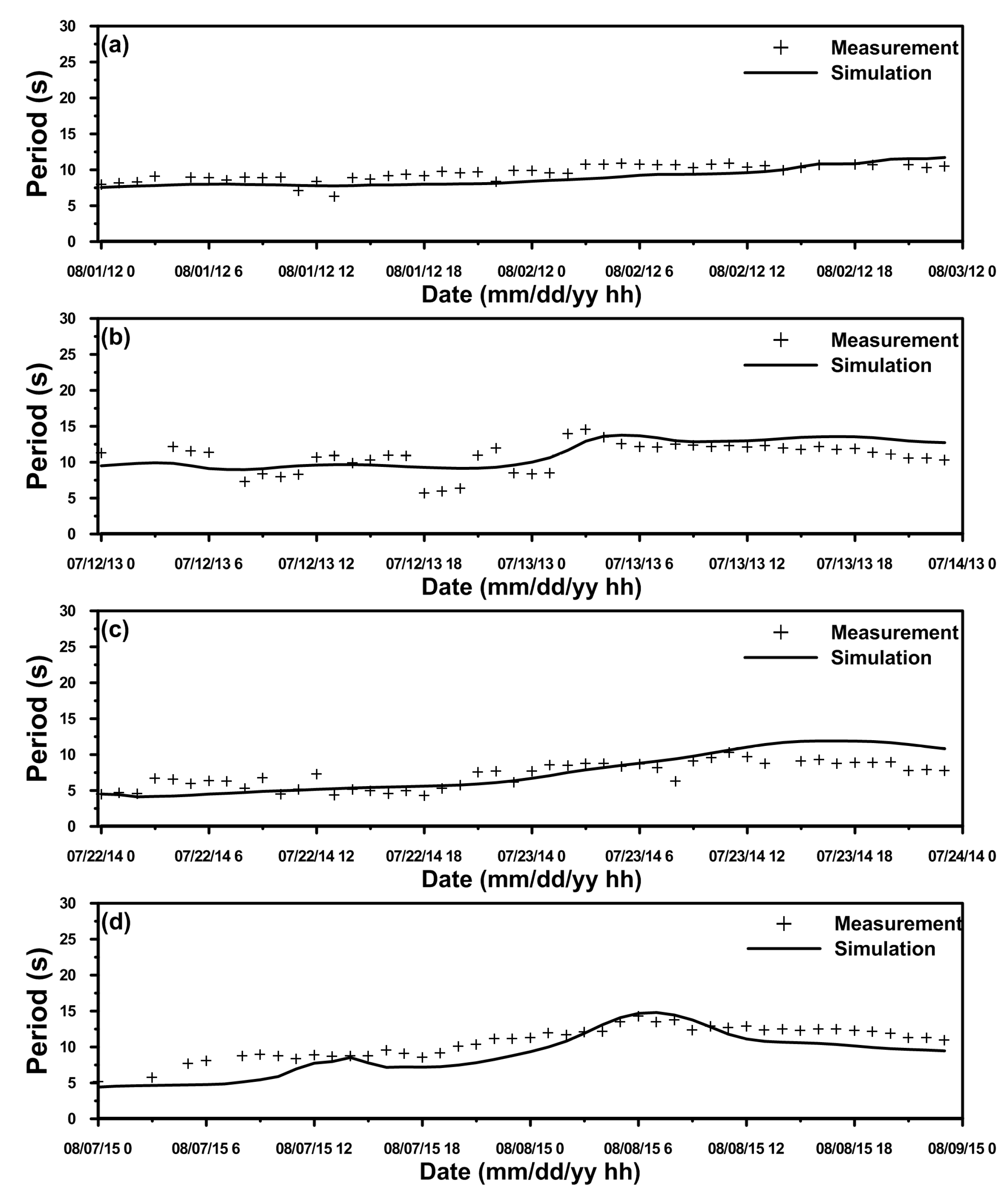
Due to the scarcity of measured wave direction date at the Keelung buoy, Suao buoy and Hualien buoy and measured wave period data at the Suao buoy and Hualien Buoy, model-observation comparisons of wave parameters were only conducted for wave height at the Keelung buoy, Suao buoy and Hualien buoy and for wave period at the Keelung buoy. It should be noted that the simulated and measured wave height and wave period are significant wave height and peak period. These two wave parameters are often specified in the measurement of sea states.
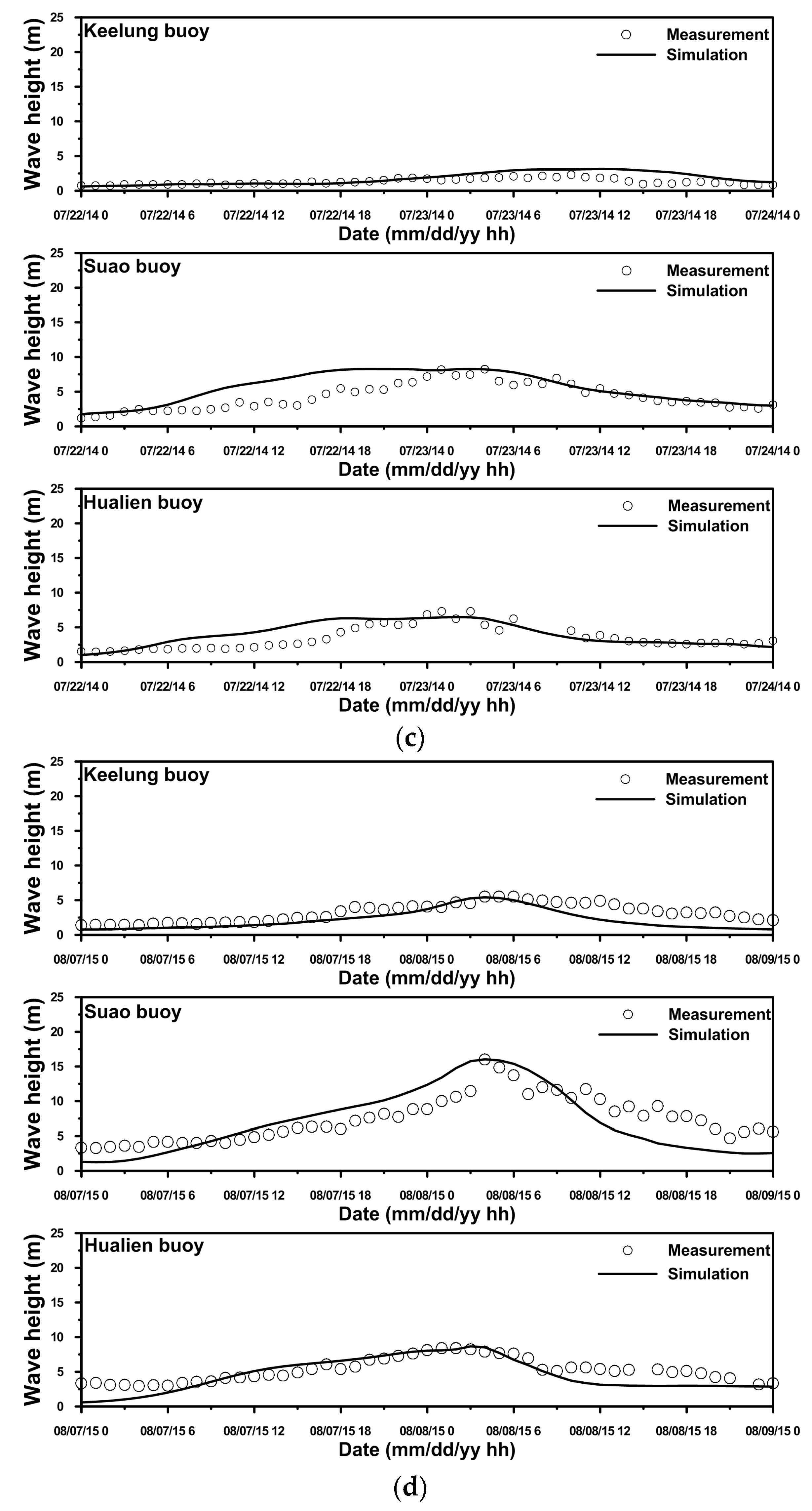
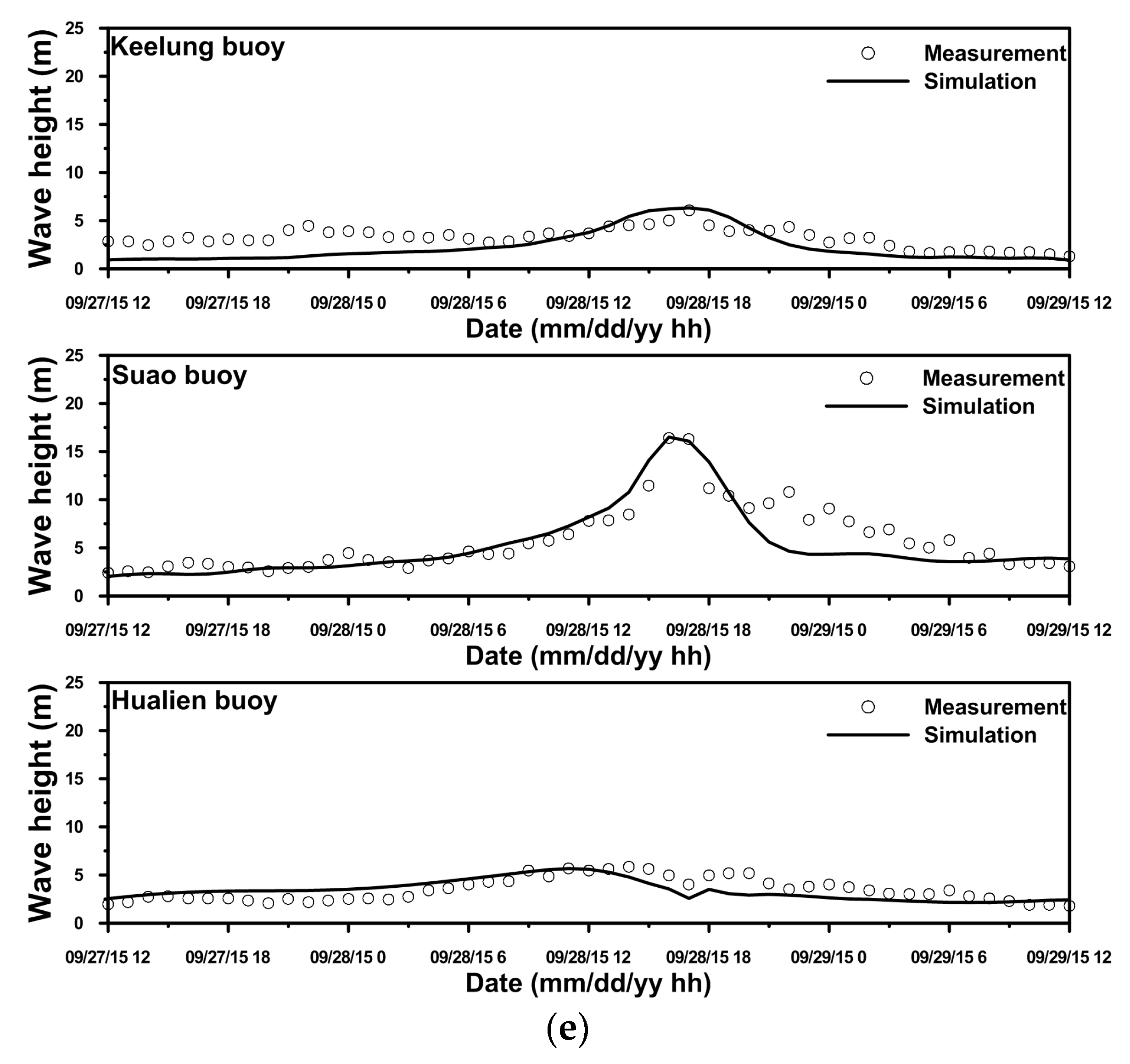
The comparisons of wave height between the simulation and observations at the Keelung buoy, Suao buoy and Hualien buoy for the five typhoon events are shown in Figure 5. The wave heights increased as the typhoon approached and decreased when typhoon was far away. The largest measured wave height exceeded 16 m at the Suao buoy during Typhoon Soudelor (2015) and Typhoon Dujuan (2015) (Figure 5d,e). The wave height measured at the Keelung buoy was almost 10 m during Typhoon Soulik (2013), while wave heights of 7.5 m were recorded during Typhoon Matmo (2014) and Typhoon Soudelor (2015) at Hualien buoy. The coupled model can only catch the peak values well but fails to mimic the measured wave heights around peak waves because the wind fields are not very accurate. Figure 6 represents the results of comparing the simulated and measured wave period at the Keelung buoy. As the typhoon passed, the wave periods also gradually increased. The maximum wave period is approximately 13 s during the period of Typhoon Soudelor (2015). Table 2 summarizes the statistical errors for wave height and wave period. The maximum wave period MAE, RMSE and PBIAS are 1.27 m, 1.56 m and 12.41% at the Suao buoy for wave height and 1.31 s, 1.51 s and −9.62% at the Keelung buoy, respectively. Overall, our tide–surge–wave coupled model demonstrates a great performance in simulating storm tides and wave heights. The best-simulated wave height, wave period and water level results were produced with a Manning coefficient set equal to 0.025. The Manning coefficient was a constant in the model due to the scarcity of type of the sea-bottom material. However, the bottom drag coefficient is varied with .
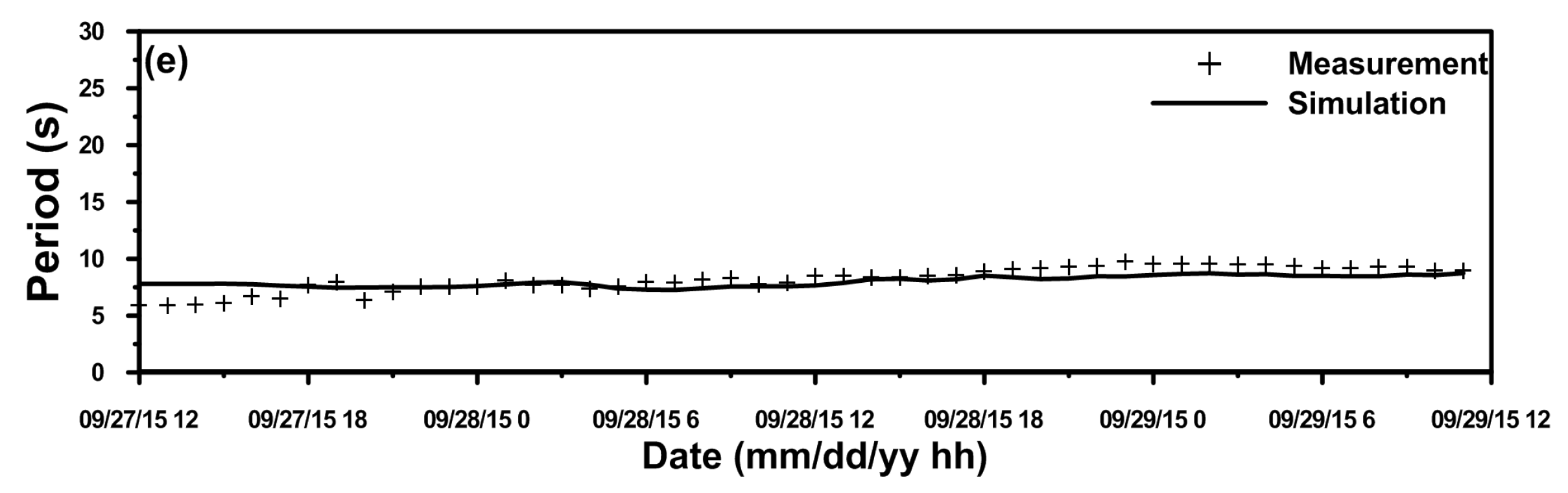
The spatial distributions of wave height predicted by WWM-II during Typhoon Soudelor (2015) are shown in Figure 7. The extent of wave height over 18 m increases as the typhoon moved northwestward. The maximum wave heights appear in the right forward quadrant of the typhoon center. This is due to the enhancement of wind velocity along the right side of typhoon by adding the typhoon translation speed [58].
5. Results and Discussion
The storm tide is caused by several components, including the astronomical tide, the low-pressure of typhoons, the wind stress of typhoons, the wave setup and the Coriolis force [59]. In the present study, three numerical experiments (as shown in Table 3) were conducted to investigate the contribution of air pressure, wind stress and waves to the storm tide at three tide gauge stations (Figure 3) during Typhoon Soudelor (2015). The baseline is a full coupled modeling; Case 1 is a decoupled modeling in which only the wave-induced radiation stress was not included; Case 2 is a decoupled modeling in which the wave-induced radiation stress and wind stress were not included; and Case 3 is a decoupled modeling in which the wave-induced radiation stress and air pressure were not included.
5.1. Effects of Waves on Storm Tides
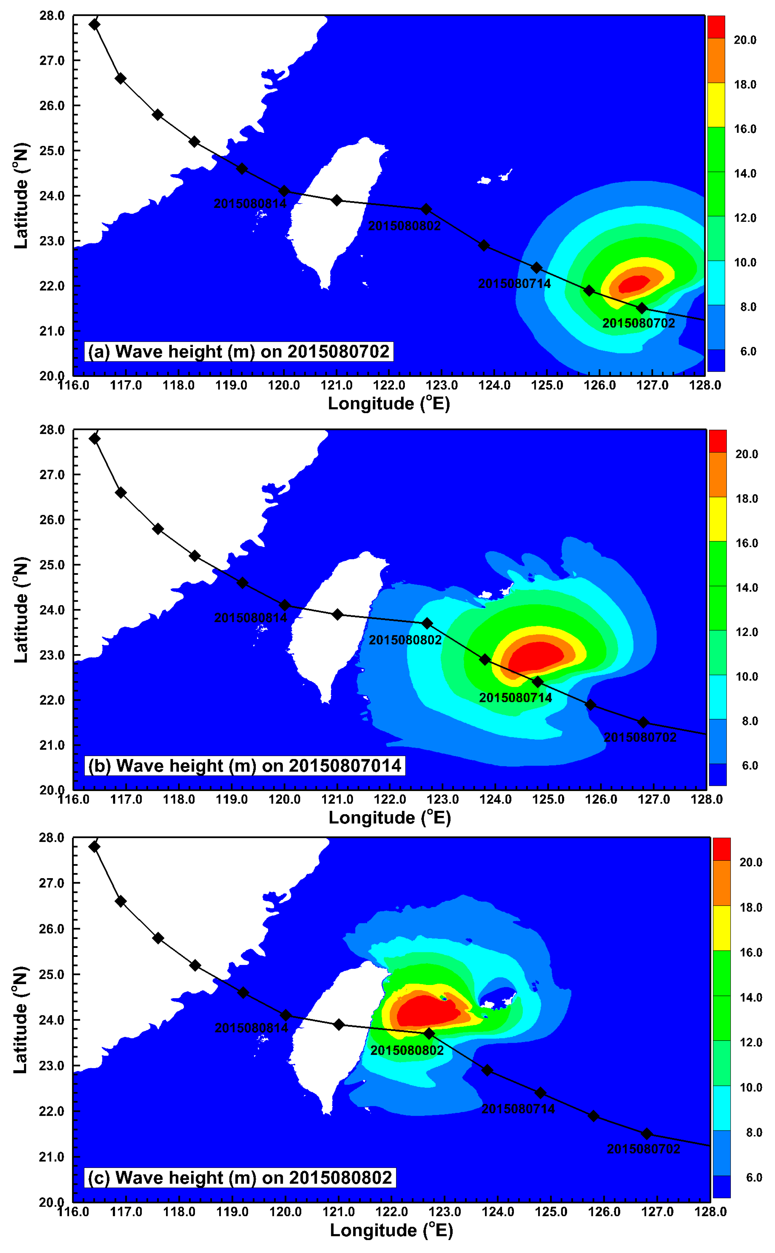
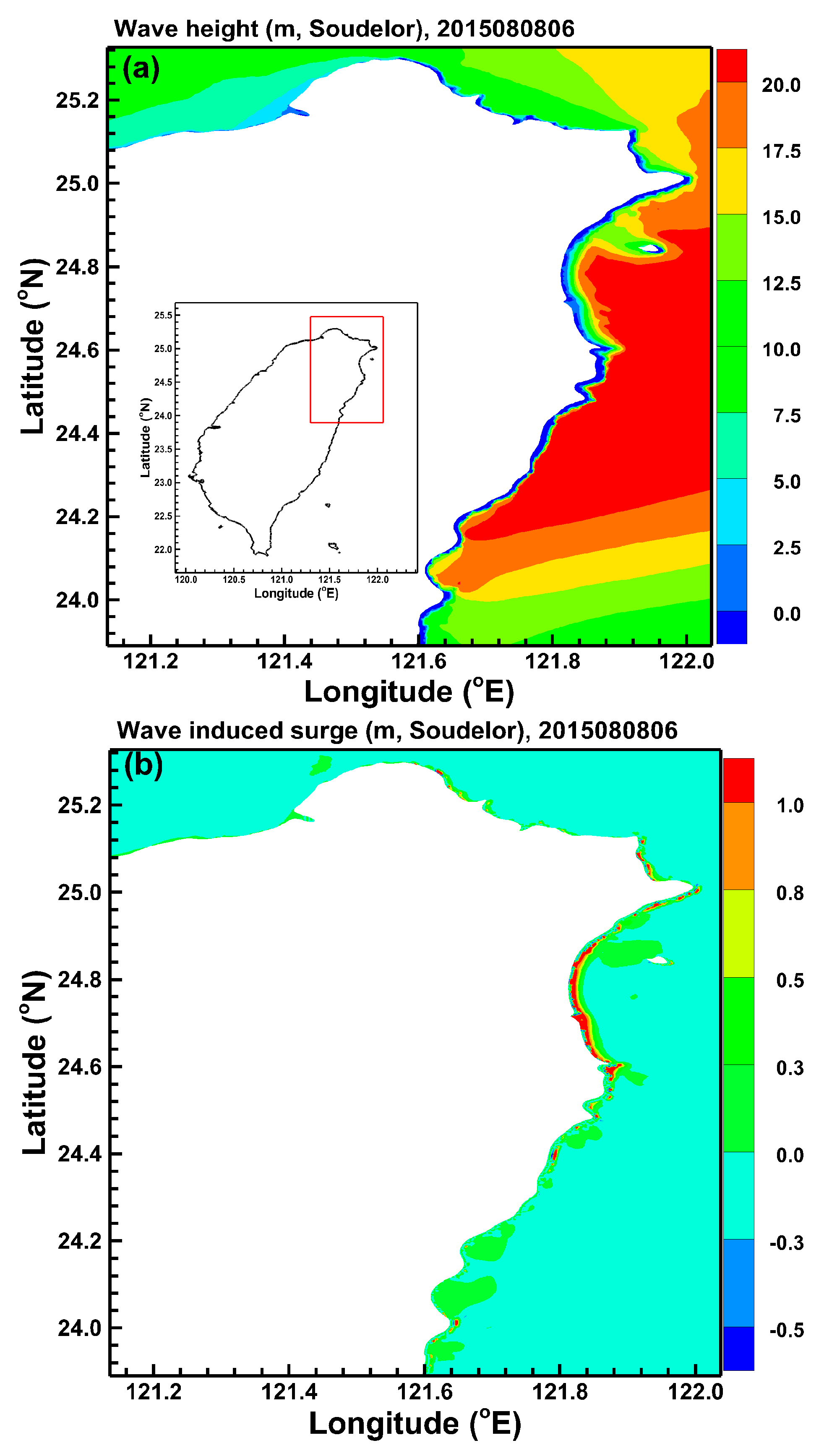
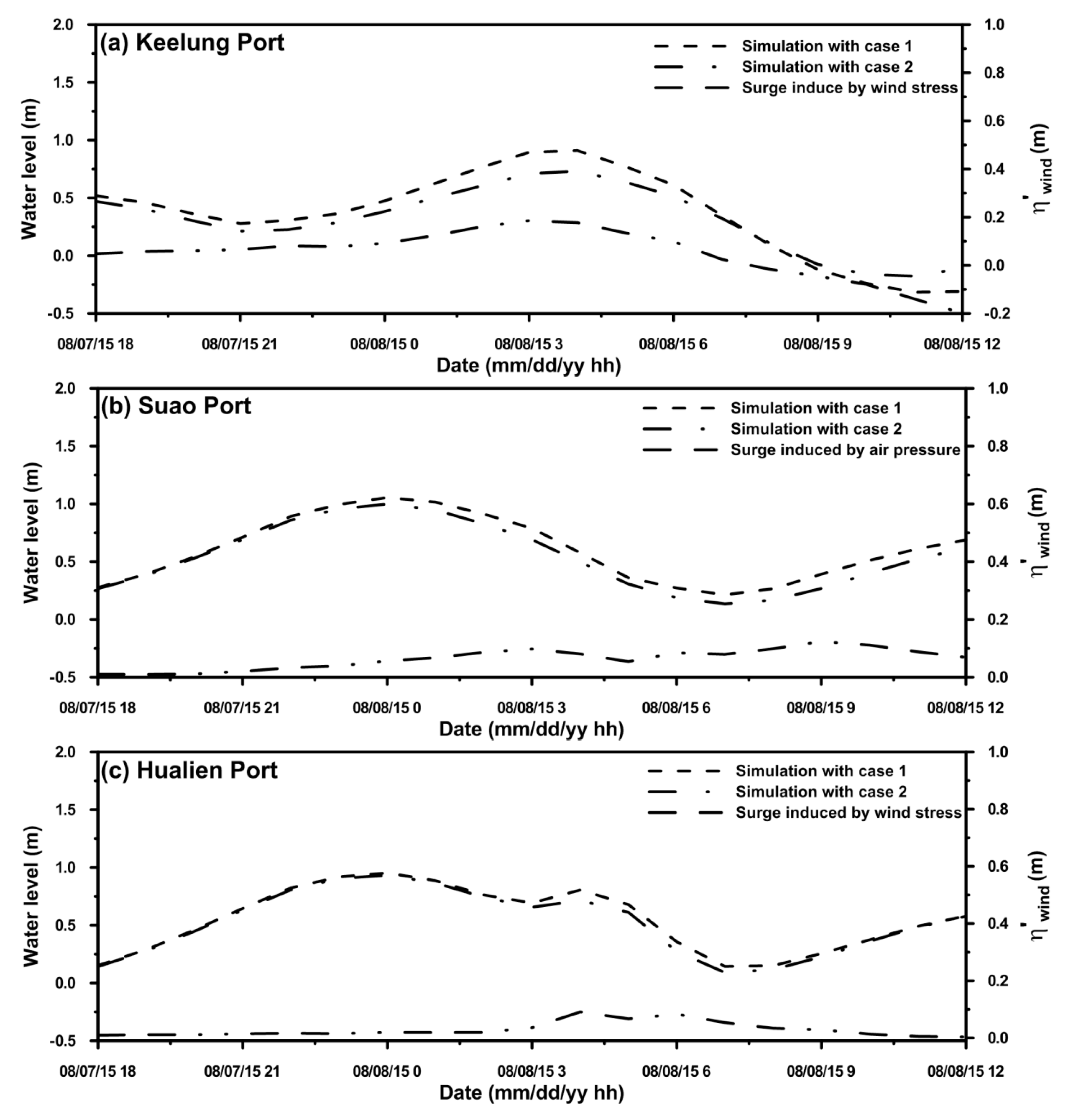
The wave-induced surge (wave setup, ) was computed by subtracting the results of Case 1 from that of the baseline. Figure 8 present the comparison of the simulated water level between the baseline and Case 1 at three tide gauge stations, and the time series of is also depicted. The contributions of to the storm tide are quite different at the three tide gauge stations. The appears to be non-significant at Keelung Port and Hualien Port (Figure 8a,c), but it is nonetheless significant, reaching 0.55 m at Suao Port (Figure 8b). The spatial distributions of wave height and are shown in Figure 9. The can be as high as 1.0 m along the coastline in relatively shallow areas, (Figure 9b) because of the offshore giant wave (Figure 9a). Huang et al. [18] found that the wave-induced forces result in an additional 0.3–0.5 m of surge relative to surge-only simulation for an Ivan-like hurricane impacting Tampa Bay, Florida. Bertin et al. [7] concluded that the maximum wave setup exceeds 0.3 and 0.4 m in the Bay of Biscay, France during the extra-tropical storms Xynthia and Joachim. The result obtained in this study is similar to their findings and reveals that the wave-induced surge is significant and essential for storm tide modeling when large wave heights occur in a region with a steep sea-bottom slope [17,60,61,62].
5.2. Effects of Wind Stress on Storm Tides
The simulations of Case 2 were compared against those of Case 1 to evaluate the contribution of wind-induced surge () to the storm tide (Figure 10). A larger of almost 0.22 m can be found at Keelung Port (Figure 10a), while weak contributions of are at Suao Port and Hualien Port (Figure 10b,c). A simple one-dimensional equation (as shown in Equation (24)) can be used to represent the [57]:
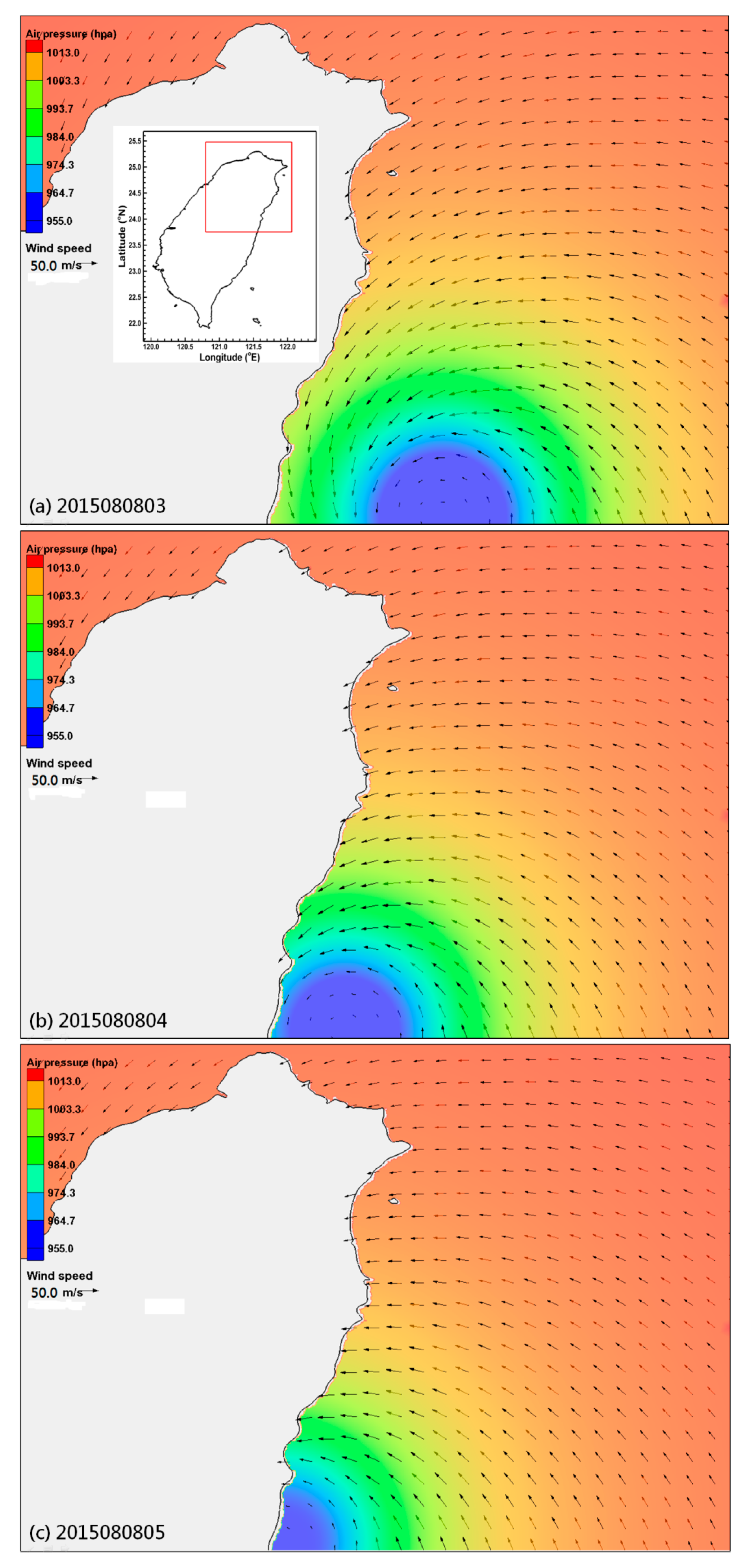
As the total water depth () becomes shallow, the wind-induced surge () is larger for the same wind stress. The sea-bottom elevations in the region of Keelung Port are shallower compared to those around Suao Port and Hualien Port (Figure 1a). The wind direction was onshore at Keelung Port during the approach of Typhoon Soudelor (2015) (Figure 11a,b). The effect of wind stress on storm tide would be significant in the shallow water area with onshore wind. According to the results derived in Section 5.1 and Section 5.2, it is concluded that the typhoon-induced wind wave would be larger along coast with the steep sea-bottom slope, for instance in the eastern coast of Taiwan, while the wind-induced surge would be smaller there.
5.3. Effects of Air Pressure on Storm Tides
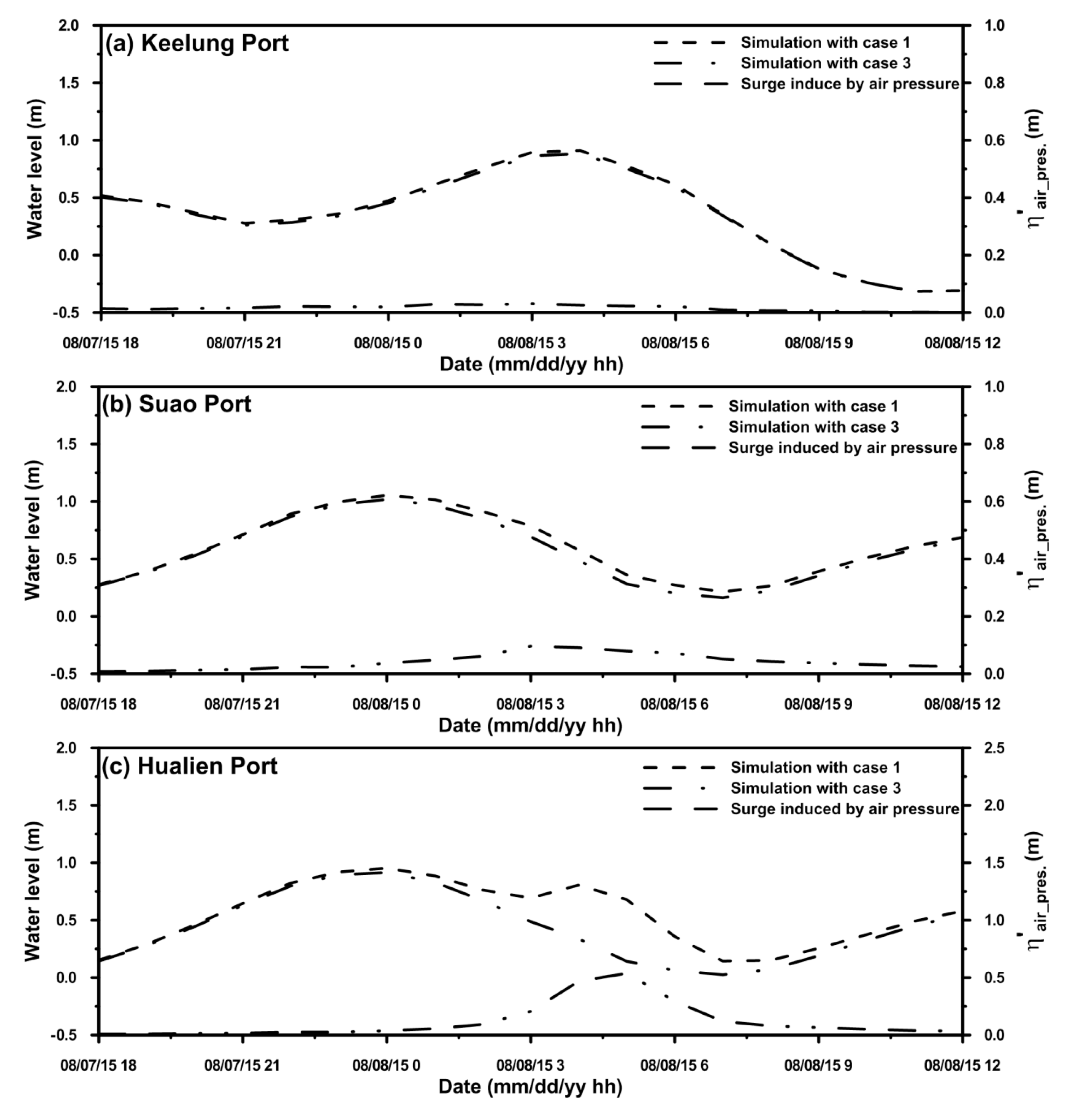
Figure 12 illustrates the comparisons of the Case 1 and the Case 3 simulations and the surge induced by air pressure (). The largest is 0.6 m at Hualien Port but is less than 0.1 m at Keelung Port and Suao Port. Hualien Port is the station closest to the center of the typhoon when Typhoon Soudelor (2015) made landfall and was thus exposed to the lowest air pressure. The can also be estimated using a simple formula based on the inverted barometer effect [60]:
5.4. Future Work
This is a preliminary study for the simulation of storm tide along the coast of Taiwan using a coupled tide–surge–wave modeling system. A further application modeling the coastal inundation associated with typhoons will be performed using high-spatial resolution grids to properly represent the natural barriers and seawalls. Using a three-dimensional coupled tide–surge–wave modeling system would likely be close to reality [63] and allow a proper representation of the vertical circulation that occurs in breaking zones [7]. Therefore, a three-dimensional coupled model should be applied to forecast the astronomical tide, storm tide and wave heights along the coast of Taiwan. Besides, the parametric cyclone model is insufficient for an accurate representation of the structure of a typhoon. Therefore the numerical weather model, such as WRF (Weather Research and Forecasting) model, is essential for storm tide modeling or forecasting in the near future.
6. Conclusions
A two-dimensional hydrodynamic (SELFE-2DH) and wind wave (WWM-II) coupled modeling system (SELFE-WWM-II) was applied to hindcast the storm tide and waves induced by typhoons for the northeastern coast of Taiwan. The detailed comparisons generally show good agreement between the model simulations and the available data measured at tide gauge stations and wave buoys. The numerical experiments were designed to analyze the contributions of waves, wind stress and air pressure to the storm tide associated with Typhoon Soudelor (2015) using a well-calibrated SELFE-WWM-II model. The results reveal that the wave-induced surge could reach to 0.55 m at Suao Port due to the offshore giant wind wave (exceeding 16.0 m) and its steep sea-bottom slope. The effects of wind stress were only slightly significant at Keelung Port, contributing 0.22 m to the storm tide as a result of shallow water and onshore wind. The air pressure results in a 0.6 m surge at Hualien Port because of the inverted barometer effect. It must be noted that the influence of waves, wind stress and air pressure on storm tides is also highly dependent on the track of the typhoon. However, it is concluded that waves should not be omitted in modeling typhoon-induced storm tides. In addition, accurate tidal and meteorological forces are indispensable in suppressing inaccuracies in storm tide predictions. Moreover, more detailed wave data from offshore buoys are needed to elucidate and verify the simulated wave dynamics in the coastal waters of Taiwan.
Acknowledgments
This research was supported by the Ministry of Science and Technology (MOST), Taiwan, grant No. MOST 105-2625-M-865-002. The authors thank the Harbor and Marine Technology Center, Taiwan for providing the measured data and Joseph Zhang at the Virginia Institute of Marine Science, College of William & Mary, and Aron Roland at the Institute for Hydraulic and Water Resources Engineering, Technische Universität Darmstadt, for kindly sharing their experiences with using the numerical model.
Author Contributions
Lee-Yaw Lin, Jiun-Huei Jang, Chih-Hsin Chang and Wei-Bo Chen conceived the study and collected measurements; and Wei-Bo Chen performed the model simulations. The final manuscript has been read and approved by all authors.
Conflicts of Interest
The authors declare no conflict of interest.
References
- Tolman, H.L. Effects of tides and storm surges on North Sea wind waves. J. Phys. Oceanogr. 1991, 21, 766–781. [Google Scholar] [CrossRef]
- Zhang, M.Y.; Li, Y.S. The synchronous coupling of a third-generation wave model and a two-dimensional storm surge model. Ocean Eng. 1996, 6, 533–543. [Google Scholar] [CrossRef]
- Xie, L.; Wu, K.; Pietrafesa, L.J.; Zhang, C. A numerical study of wave-current interaction through surface and bottom stresses: Wind-driven circulation in the South Atlantic Bight under uniform winds. J. Geophys. Res. 2001, 106, 16841–16855. [Google Scholar] [CrossRef]
- Xie, L.; Pietrafesa, L.J.; Wu, K. A numerical study of wave-current interaction through surface and bottom stresses: Coastal ocean response to Hurricane Fran of 1996. J. Geophys. Res. 2003, 108, 3049. [Google Scholar] [CrossRef]
- Jennifer, M.B. A case study of combined wave and water levels under storm conditions using WAM and SWAN in a shallow water application. Ocean Model. 2010, 35, 215–229. [Google Scholar]
- Sun, Y.; Chen, C.; Beardsley, R.C.; Xu, Q.; Qi, J.; Lin, H. Impact of current-wave interaction on storm surge simulation: A case study for Hurricane Bob. J. Geophys. Res. 2013, 118, 2685–2701. [Google Scholar] [CrossRef]
- Bertin, X.; Li, K.; Roland, A.; Bidlot, J.R. The contribution of short-wave in storm surge: Two case studies in the Bay of Biscay. Cont. Shelf Res. 2015, 96, 1–15. [Google Scholar] [CrossRef]
- Flather, R.A.; Proctor, R.; Wolf, J. Oceanographic forecast models. In Computer Modeling in the Environmental Sciences; IMA Conference Series 28; Famer, D.G., Rycroft, M.J., Eds.; Clarendon Press: Oxford, UK, 1991; pp. 15–30. [Google Scholar]
- Jelesnianski, C.P.; Chen, J.; Shaffer, W.A. SLOSH: Sea, Lake, and Overland Surges from Hurricane; National Weather Service: Silver Springs, MD, USA, 1992.
- Luettich, R.A.; Westerink, J.J.; Scheffner, N.W. ADCIRC: An Advanced Three-Dimensional Circulation Model for Shelves, Coasts, and Estuaries, Report I: Theory and Methodology of ADCIRC-2DDI and ADCIRC-3DL; Technical Report DRP-92-6; U.S. Army Corps of Engineers: Vicksburg, MS, USA, 1992.
- Verboom, G.K.; Ronde, J.G.; Van Dijk, R.P. A fine grid tidal flow and storm surge model of the North Sea. Cont. Shelf Res. 1992, 12, 213–233. [Google Scholar] [CrossRef]
- Westerink, J.J.; Luettich, R.A.; Baptista, A.M.; Scheffner, N.W.; Farrar, P. Tide and storm surge predictions using a finite element model. J. Hydraul. Eng. 1992, 118, 1373–1390. [Google Scholar] [CrossRef]
- Hubbert, G.D.; McInnes, K.L. A storm surge inundation model for coastal planning an impact studies. J. Coast. Res. 1999, 15, 168–185. [Google Scholar]
- Dube, S.K.; Chittibabu, P.; Sinha, P.C.; Rao, A.D.; Murty, T.S. Numerical modeling of storm surge in the head Bay of Bengal using location specific model. Nat. Hazards 2004, 31, 437–453. [Google Scholar] [CrossRef]
- Dietsche, D.; Hagen, S.C.; Bacopoulos, P. Storm surge simulation for Hurricane Hugo (1989), on the significance of inundation areas. J. Waterw. Port Coast Ocean Eng. 2007, 133, 183–191. [Google Scholar] [CrossRef]
- Chen, W.B.; Liu, W.C.; Hsu, M.H. Computational investigation of typhoon-induced storm surges along the Coast of Taiwan. Nat. Hazards 2012, 64, 1161–1185. [Google Scholar] [CrossRef]
- Resio, D.T.; Westerink, J.J. Modeling the physics of storm surges. Phys. Today 2008, 61, 33. [Google Scholar] [CrossRef]
- Huang, Y.; Weisberg, R.H.; Zheng, L. Coupling of surge and waves for an Ivan-like hurricane impacting the Tampa Bay, Florida region. J. Geophys. Res. 2010, 115, C12009. [Google Scholar] [CrossRef]
- Sebastian, A.; Proft, J.; Dietrich, J.C.; Du, W.; Bedient, P.B.; Dawson, C.N. Characterizing hurricane storm surge behavior in Galveston Bay using the SWAN+ADCRIC model. Coast. Eng. 2014, 88, 171–181. [Google Scholar] [CrossRef]
- Zhao, C.; Ge, J.; Ding, P. Impact of sea level rise on storm surges around the Changjiang estuary. J. Coast. Res. 2014, 68, 27–34. [Google Scholar] [CrossRef]
- Lee, H.S.; Kim, K.O. Storm surge and storm waves mideling due to Typhoon Haiyan in November 2013 with improve dynamic meteorological conditions. Procedia Eng. 2015, 116, 699–706. [Google Scholar] [CrossRef]
- Yoon, J.-J.; Jun, K.-C. Coupled storm surge and wave simulations for the southern coast of Korea. Ocean Sci. J. 2015, 50, 9–28. [Google Scholar] [CrossRef]
- Amante, C.; Eakins, B.W. ETOPO1 1 Arc-Minute Global Relief Model: Procedures, Data Sources and Analysis. NOAA Technical Memorandum NESDIS NGDC-24; National Geophysical Data Center Marine Geology and Geophysics Division Boulder, Colorado: Boulder, CO, USA, 2009. [CrossRef]
- Zhang, Y.J.; Baptista, A.M. SELFE: A semi-implicit Eulerian-Lagrangian finite-element model for cross-scale ocean circulation. Ocean Model. 2008, 21, 71–96. [Google Scholar] [CrossRef]
- Roland, A. Development of WWM II: Spectral Wave Modelling on Unstructured Meshes. Ph.D. Thesis, Technische Universität Darmstadt, Darmstadt, Germany, 2008. [Google Scholar]
- Roland, A.; Zhang, Y.J.; Wang, H.V.; Meng, Y.; Teng, Y.-C.; Maderich, V.; Brovchenko, I.; Dutour-Sikiric, M.; Zanke, U. A fully coupled 3D wave-current interaction model on unstructured grids. J. Geophys. Res. 2012, 117, C00J33. [Google Scholar] [CrossRef]
- Hasselmann, K.; Barnett, T.P.; Bouws, E.; Carlson, H.; Cartwright, D.E.; Enke, K. Measurements of wind-wave growth and swell decay during the Joint North Sea Wave Project (JONSWAP). Dtsch. Hydrogr. Z. 1973, 12, 1–95. [Google Scholar]
- Battjes, J.A.; Janssen, J.P.F.M. Energy loss and set-up due to breaking of random waves. In Proceedings of the 16th International Conference on Coastal Engineering, Hamburg, Germany, 27 August–3 September 1978; pp. 569–587. [Google Scholar]
- Zhang, Y.J.; Witter, R.C.; Priest, G.R. Tsunami-tide interaction in 1964 Prince William Sound tsunami. Ocean Model. 2011, 40, 246–259. [Google Scholar] [CrossRef]
- Rodrigues, M.; Oliveira, A.; Queiroga, H.; Fortunato, A.B.; Zhang, Y.J. Three-dimensional modeling of the lower trophic levels in the Ria de Aveiro (Portugal). Ecol. Model. 2009, 220, 1274–1290. [Google Scholar] [CrossRef]
- Rodrigues, M.; Oliveira, A.; Guerreior, M.; Fortunato, A.B.; Menaia, J.; David, L.M.; Cravo, A. Modeling fecal contamination in the Aljezur coastal stream (Portugal). Ocean Dyn. 2011, 61, 841–856. [Google Scholar] [CrossRef]
- Azevedo, A.; Oliveira, A.; Fortunato, A.B.; Bertin, X. Application of an Eulerian-Lagrangian oil spill modeling system to the prestige accident: Trajectory analysis. J. Coast. Res. 2011, 777–781. [Google Scholar]
- Fortunato, A.B.; Rodrigues, M.; Dias, J.M.; Lopes, C.; Oliveira, A. Generating inundation maps for a coastal lagoon: A case study in the Ria de Aveiro (Portugal). Ocean Eng. 2013, 64, 60–71. [Google Scholar] [CrossRef]
- Chen, W.B.; Liu, W.C. Assessment of storm surge inundation and potential hazard maps for the southern coast of Taiwan. Nat. Hazards 2016, 82, 591–616. [Google Scholar] [CrossRef]
- Chen, W.B.; Liu, W.C. Modeling flood inundation Induced by river flow and storm surges over a river basin. Water 2014, 6, 3182–3199. [Google Scholar] [CrossRef]
- Wang, H.V.; Loftis, J.D.; Liu, Z.; Forrest, D.; Zhang, J. The storm surge and sub-grid inundation modeling in New York City during hurricane Sandy. J. Mar. Sci. Eng. 2014, 2, 226–246. [Google Scholar] [CrossRef]
- Powell, M.D.; Vickery, P.J.; Reinhold, T.A. Reduced drag coefficient for high wind speeds in tropical cyclones. Nature 2003, 422, 279–283. [Google Scholar] [CrossRef] [PubMed]
- Longuet-Higgins, M.S.; Stewart, R.W. Radiation stress in water waves: A physical discussion with applications. Deep Sea Res. 1964, 11, 529–562. [Google Scholar]
- Battjes, J.A. Computation of Set-up, Longshore Currents, Run-up and Overtopping Due to Wind-Generated Waves. Ph.D. Thesis, Department of Civil Engineering, Delft University of Technology, Delft, The Netherlands, 1974. [Google Scholar]
- Chen, Q.; Wang, L.; Zhao, H.; Douglass, S.L. Predictions of storm surges and wind waves on coastal Highways in hurricane-prone areas. J. Coast. Res. 2007, 23, 1304–1317. [Google Scholar] [CrossRef]
- Egbert, G.D.; Bennett, A.F.; Foreman, M.G.G. Topex/poseidon tides estimated using a global inverse model. J. Geophys. Res. 1994, 99, 821–852. [Google Scholar] [CrossRef]
- Egbert, G.D.; Erofeeva, S.Y. Efficient inverse modeling of barotropic ocean tides. J. Atmos. Ocean. Technol. 2002, 19, 183–204. [Google Scholar] [CrossRef]
- Fujita, T. Pressure distribution in typhoon. Geophys. Mag. 1952, 23, 437. [Google Scholar]
- Jelesnianski, C.P. A numerical computation of storm tides induced by a tropical storm impinging on a continental shelf. Mon. Weather Rev. 1965, 93, 343–358. [Google Scholar] [CrossRef]
- Holland, G.J. An analytical model of the wind and pressure profiles in hurricanes. Mon. Weather Rev. 1980, 108, 1212–1218. [Google Scholar] [CrossRef]
- Wang, X.; Qian, C.; Wang, W.; Yan, T. An elliptical wind field model of typhoons. J. Ocean Univ. China 2004, 3, 33–39. [Google Scholar] [CrossRef]
- MacAfee, A.W.; Pearson, G.W. Development and testing of tropical Cyclone parametric wind models tailored for midlatitude application-preliminary results. J. Appl. Meteorol. Climatol. 2006, 45, 1244–1260. [Google Scholar] [CrossRef]
- Wood, V.T.; White, L.W.; Willoughby, H.E.; Jorgensen, D.P. A new parametric tropical cyclone tangential wind profile model. Mon. Weather Rev. 2013, 141, 1884–1909. [Google Scholar] [CrossRef]
- Jakobsen, F.; Madsen, H. Comparison and further development of parametric tropical cyclone models for storm surge modelling. J. Wind Eng. Ind. Aerodyn. 2004, 92, 375–391. [Google Scholar] [CrossRef]
- Lin, N.; Chavas, D. On hurricane parametric wind and applications in storm surge modeling. J. Geophys. Res. 2012, 117, D09120. [Google Scholar] [CrossRef]
- Hubbert, G.D.; Holland, G.J.; Leslie, L.M.; Manton, M.J. A real-time system for forecasting tropical cyclone storm surges. Weather Forecast. 1991, 6, 86–97. [Google Scholar] [CrossRef]
- Zhang, H.; Sheng, J. Examination of extreme sea levels due to storm surges and tides over the northwest Pacific Ocean. Cont. Shelf Res. 2015, 93, 81–97. [Google Scholar] [CrossRef]
- Georgiou, P. Design Wind Speeds in Tropical Cyclone Prone Regions. Ph.D. Thesis, University of Western Ontario, London, ON, Canada, 1985. [Google Scholar]
- Phake, A.C.L.; Martion, C.D.; Cheung, K.F.; Souston, S.H. Modeling of tropical cyclone winds and waves for emergency management. Ocean Eng. 2003, 30, 553–578. [Google Scholar] [CrossRef]
- Gupta, H.V.; Sorooshian, S.; Yapo, P.O. Status of automatic calibration for hydrologic models: Comparison with multilevel expert calibration. J. Hydrol. Eng. 1999, 4, 135–143. [Google Scholar] [CrossRef]
- Moriasi, D.N.; Arnold, J.G.; Van Liew, M.W.; Bingner, R.L.; Harmel, R.D.; Veith, T.L. Model evaluation guidelines for systematic quantification of accuracy in watershed simulations. Am. Soc. Agric. Biol. Eng. 2007, 50, 885–900. [Google Scholar]
- Feng, W.; Yin, B.; Yang, D. Effect of hurricane paths on storm surge response at Tianjin, China. Estuar. Coast. Shelf Sci. 2012, 106, 58–68. [Google Scholar] [CrossRef]
- Moon, I.-J.; Ginis, I.; Hara, T.; Tolman, H.; Wright, C.W.; Walsh, E.J. Numerical simulation of sea-surface directional wave spectra under hurricane wind forcing. J. Phys. Oceanogr. 2003, 33, 1680–1706. [Google Scholar] [CrossRef]
- Dean, R.G.; Dalrymple, R.A. Coastal Processes with Engineering Applications; Cambridge University Press: Cambridge, UK, 2002. [Google Scholar]
- Wolf, J. Coupled wave and surge modelling and implications for coastal flooding. Adv. Geosci. 2008, 17, 19–22. [Google Scholar] [CrossRef]
- Dietrich, J.C.; Zijlema, M.; Westerink, J.J.; Holthuijsen, L.H.; Dawson, C.; Luettich, R.A., Jr.; Jesen, R.E.; Smith, J.M.; Stelling, G.S.; Stone, G.W. Modeling hurricane wave and storm surge using integrally-couple scalable computations. Coast. Eng. 2011, 58, 45–65. [Google Scholar] [CrossRef]
- Vatvani, D.; Zweers, N.C.; van Ormondt, M.; Smale, A.J.; de Vries, H.; Makin, V.K. Storm surge and wave simulations in the Gulf of Mexico using a consistent drag relation for atmospheric and storm surge model. Nat. Hazards Earth Syst. Sci. 2012, 12, 2399–2410. [Google Scholar] [CrossRef]
- Bruneau, N.; Dodet, G.; Bertin, X.; Fortunato, A.B. Development of a three-dimensional coupled wave-current model for coastal environments. J. Coast. Res. 2011, 64, 986–990. [Google Scholar]
Figure 1.
(a) Bathymetry and (b) unstructured grids for the computational domain.


Figure 2.
Schematic diagram for the coupled model.

Figure 3.
Tracks of typhoons and locations of tidal gauge stations and wave buoy stations used for model validation.
Figure 3.
Tracks of typhoons and locations of tidal gauge stations and wave buoy stations used for model validation.

Figure 4.
Comparisons of modeled and observed water levels during: (a) Typhoon Saola in 2012; (b) Typhoon Soulik in 2013; (c) Typhoon Matmo in 2014; (d) Typhoon Soudelor in 2015; and (e) Typhoon Dujuan in 2015.
Figure 4.
Comparisons of modeled and observed water levels during: (a) Typhoon Saola in 2012; (b) Typhoon Soulik in 2013; (c) Typhoon Matmo in 2014; (d) Typhoon Soudelor in 2015; and (e) Typhoon Dujuan in 2015.


Figure 5.
Comparisons of modeled and observed wave heights during: (a) Typhoon Saola in 2012; (b) Typhoon Soulik in 2013; (c) Typhoon Matmo in 2014; (d) Typhoon Soudelor in 2015; and (e) Typhoon Dujuan in 2015.
Figure 5.
Comparisons of modeled and observed wave heights during: (a) Typhoon Saola in 2012; (b) Typhoon Soulik in 2013; (c) Typhoon Matmo in 2014; (d) Typhoon Soudelor in 2015; and (e) Typhoon Dujuan in 2015.
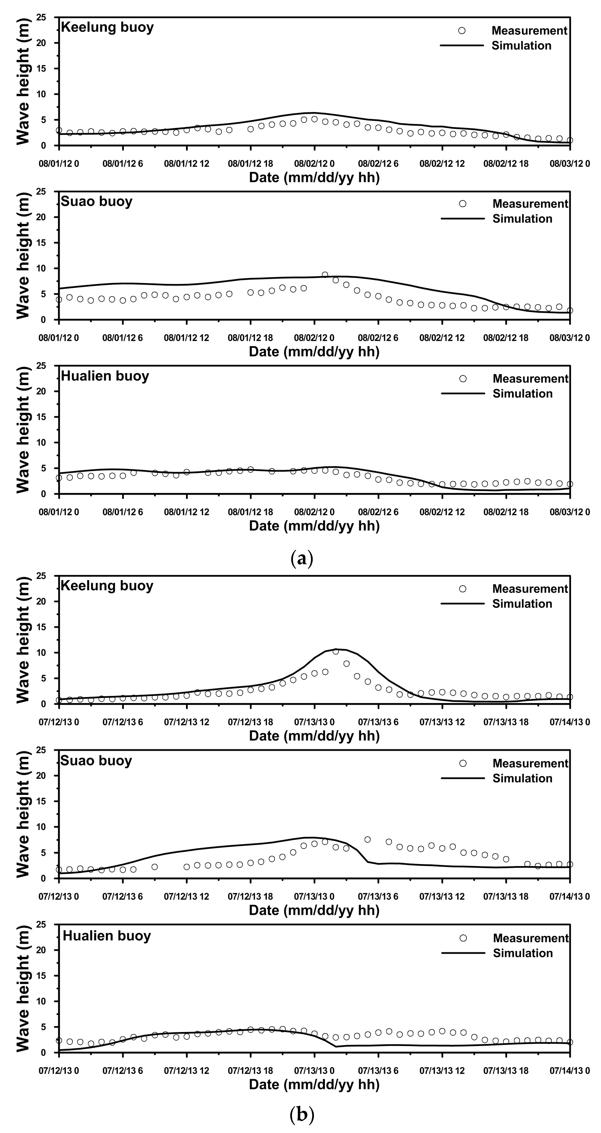


Figure 6.
Comparisons of modeled and observed wave periods during: (a) Typhoon Saola (2012); (b) Typhoon Soulik (2013); (c) Typhoon Matmo (2014); (d) Typhoon Soudelor (2015); and (e) Typhoon Dujuan (2015) at the Keelung buoy.
Figure 6.
Comparisons of modeled and observed wave periods during: (a) Typhoon Saola (2012); (b) Typhoon Soulik (2013); (c) Typhoon Matmo (2014); (d) Typhoon Soudelor (2015); and (e) Typhoon Dujuan (2015) at the Keelung buoy.


Figure 7.
Spatial distribution of simulated wave height along the track of the typhoon at: (a) 02:00 on 7 August 2015, (b) 14:00 on 7 August 2015; and (c) 02:00 on 8 August 2015 for Typhoon Soudelor (2015).
Figure 7.
Spatial distribution of simulated wave height along the track of the typhoon at: (a) 02:00 on 7 August 2015, (b) 14:00 on 7 August 2015; and (c) 02:00 on 8 August 2015 for Typhoon Soudelor (2015).

Figure 8.
Comparison of the simulated water level between the baseline and Case 1 and calculated wave-induced surge at: (a) Keelung Port; (b) Suao Port; and (c) Hualien Port during Typhoon Soudelor (2015).
Figure 8.
Comparison of the simulated water level between the baseline and Case 1 and calculated wave-induced surge at: (a) Keelung Port; (b) Suao Port; and (c) Hualien Port during Typhoon Soudelor (2015).

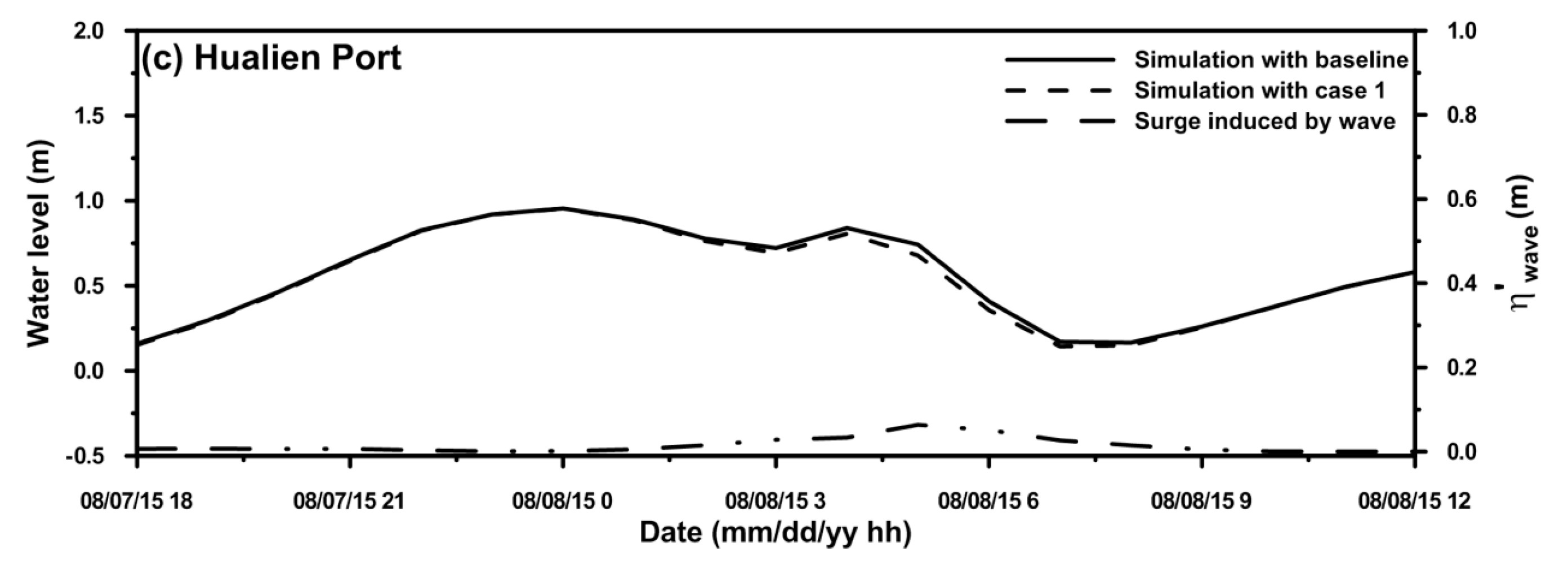
Figure 9.
Spatial distribution of simulated: (a) wave height; and (b) wave-induced surge at 06:00 on 8 August 2015 for Typhoon Soudelor (2015).
Figure 9.
Spatial distribution of simulated: (a) wave height; and (b) wave-induced surge at 06:00 on 8 August 2015 for Typhoon Soudelor (2015).

Figure 10.
Comparison of the simulated water level between Case 1 and Case 2 and the calculated wind induced surge at: (a) Keelung Port; (b) Suao Port; and (c) Hualien Port during Typhoon Soudelor (2015).
Figure 10.
Comparison of the simulated water level between Case 1 and Case 2 and the calculated wind induced surge at: (a) Keelung Port; (b) Suao Port; and (c) Hualien Port during Typhoon Soudelor (2015).

Figure 11.
Distribution of air pressure (color) and wind speed (vector) at: (a) 03:00; (b) 04:00; and (c) 05:00 on 8 August 2015 for Typhoon Soudelor (2015).
Figure 11.
Distribution of air pressure (color) and wind speed (vector) at: (a) 03:00; (b) 04:00; and (c) 05:00 on 8 August 2015 for Typhoon Soudelor (2015).

Figure 12.
Comparison of the simulated water level between Case 1 and Case 3 and the calculated air pressure-induced surge at: (a) Keelung Port; (b) Suao Port; and (c) Hualien Port during Typhoon Soudelor (2015).
Figure 12.
Comparison of the simulated water level between Case 1 and Case 3 and the calculated air pressure-induced surge at: (a) Keelung Port; (b) Suao Port; and (c) Hualien Port during Typhoon Soudelor (2015).

Table 1.
The parameters used in SELFE-WWM-II and parametric cyclone model.
| Parameters | Model | Source |
|---|---|---|
| SEFLE-WWM-II | Equation (5) | |
| SEFLE-WWM-II | Equation (14) | |
| Parametric cyclone model | 1013.0 | |
| Parametric cyclone model | From RSMC dataset | |
| Parametric cyclone model | Equation (18) | |
| Parametric cyclone model | Equation (19) | |
| Parametric cyclone model | Equation (20) | |
| SEFLE-WWM-II | 0.025 |
Table 2.
Statistical errors at available tidal gauge stations and wave buoys for model validation.
| Station | Wave Height | Water Level | Wave Period | ||||||
|---|---|---|---|---|---|---|---|---|---|
| MAE (m) | RMSE (m) | PBIAS (%) | MAE (m) | RMSE (m) | PBIAS (%) | MAE (s) | RMSE (s) | PBIAS (%) | |
| Keeling | 1.07 | 1.26 | −5.41 | 0.11 | 0.12 | 9.86 | 1.31 | 1.51 | −9.62 |
| Suao | 1.27 | 1.56 | 12.41 | 0.10 | 0.12 | 9.98 | -- | -- | -- |
| Hualien | 0.84 | 0.97 | 4.5 | 0.09 | 0.11 | −5.38 | -- | -- | -- |
Notes: --: Observations are scarce for comparison.
Table 3.
Designed numerical experiments for investigating the factors contributing to surge.
| Simulation | Conditions | Investigated Factors |
|---|---|---|
| Baseline | Simulation with air pressure, wind stress and wave | None |
| Case 1 | Simulation only with air pressure, wind stress | Wave |
| Case 2 | Simulation only with air pressure | Wind stress |
| Case 3 | Simulation only with wind stress | Air pressure |
© 2017 by the authors. Licensee MDPI, Basel, Switzerland. This article is an open access article distributed under the terms and conditions of the Creative Commons Attribution (CC BY) license (http://creativecommons.org/licenses/by/4.0/).
Share and Cite
MDPI and ACS Style
Chen, W.-B.; Lin, L.-Y.; Jang, J.-H.; Chang, C.-H. Simulation of Typhoon-Induced Storm Tides and Wind Waves for the Northeastern Coast of Taiwan Using a Tide–Surge–Wave Coupled Model. Water 2017, 9, 549. https://doi.org/10.3390/w9070549
AMA Style
Chen W-B, Lin L-Y, Jang J-H, Chang C-H. Simulation of Typhoon-Induced Storm Tides and Wind Waves for the Northeastern Coast of Taiwan Using a Tide–Surge–Wave Coupled Model. Water. 2017; 9(7):549. https://doi.org/10.3390/w9070549
Chicago/Turabian StyleChen, Wei-Bo, Lee-Yaw Lin, Jiun-Huei Jang, and Chih-Hsin Chang. 2017. "Simulation of Typhoon-Induced Storm Tides and Wind Waves for the Northeastern Coast of Taiwan Using a Tide–Surge–Wave Coupled Model" Water 9, no. 7: 549. https://doi.org/10.3390/w9070549
Note that from the first issue of 2016, this journal uses article numbers instead of page numbers. See further details here.