A Hydrological and Geomorphometric Approach to Understanding the Generation of Wadi Flash Floods
by
 , , , and
Mohammed Abdel-Fattah
1,* ,
,
Mohamed Saber
2,3,
Sameh A. Kantoush
2,
Mohamed F. Khalil
3,
Tetsuya Sumi
2 and
Ahmed M. Sefelnasr
3 1
Graduate School of Engineering, Kyoto University, Kyoto 615-8540, Japan
2
Disaster Prevention Research Institute (DPRI), Kyoto University, Kyoto 611-0011, Japan
3
Geology Department, Assiut University, 71516 Assiut, Egypt
*
Author to whom correspondence should be addressed.
Water 2017, 9(7), 553; https://doi.org/10.3390/w9070553
Submission received: 14 June 2017
/
Revised: 16 July 2017
/
Accepted: 20 July 2017
/
Published: 24 July 2017
(This article belongs to the Special Issue Innovative Aspects in Flood Risk Evaluation, Mapping and Communication)
Abstract
:The generation and processes of wadi flash floods are very complex and are not well understood. In this paper, we investigate the relationship between variations in geomorphometric and rainfall characteristics and the responses of wadi flash floods. An integrated approach was developed based on geomorphometric analysis and hydrological modeling. The Wadi Qena, which is located in the Eastern Desert of Egypt, was selected to validate the developed approach and was divided into 14 sub-basins with areas ranging from 315 to 1488 km2. The distributed Hydrological River Basin Environment Assessment Model (Hydro-BEAM) was used to obtain a good representation of the spatial variability of the rainfall and geomorphology in the basin. Thirty-eight geomorphometric parameters representing the topographic, scale, shape and drainage characteristics of the basins were considered and extracted using geographic information system (GIS) techniques. A series of flash flood events from 1994, 2010, 2013, and 2014, in addition to synthetic virtual storms with different durations and intensities, were selected for the application of this study. The results exhibit strong correlations between scale and topographic parameters and the hydrological indices of the wadi flash floods, while the shape and drainage network metrics have smaller impacts. The total rainfall amount and duration significantly impact the relationship between the hydrologic response of the wadi and its geomorphometry. For most of the parameters, we found that the impact of the wadi geomorphometry on the hydrologic response increases with increasing rainfall intensity.
1. Introduction
Flash flood disasters occurring in the arid environment of a wadi, which means valley in Arabic, are associated with several challenges related to the unique characteristics of wadi systems, current data limitations and the use of inconsistent methods [1,2,3]. Arid wadis are characterized by the prevalence of a dry climate throughout the entire year, except during infrequent rainfall events that can produce flash floods. Costa [4] indicated that arid or semiarid environments may experience more severe floods than humid areas with greater rainfall intensity. The infrequent nature of wadi flash floods (WFFs) and the absence of efficient disaster management strategy, combined with recent unplanned development activities [5] and increased poverty, have reduced the ability of the wadi community to face such devastating disasters. In wadis, land reclamation and housing construction usually occur across the wadi channel and floodplain without undertaking the proper mitigation measures. However, floods in arid wadis are also an essential source of water, particularly for groundwater recharge.
Egypt is one of the arid countries that suffers from the effects of WFFs in the coastal and Nile River dry wadis (Figure 1). For instance, during the January 2010 floods, ten people died and hundreds of houses were destroyed in Sinai and Southern Egypt, and the May 2014 flood resulted in approximately 150 million USD of damages in Taba City. Although water demand in Egypt is increasing due to population growth and several recent development activities, Egypt’s share from the Nile River could be reduced by the completion of the planned dams in upstream countries (e.g., the Renaissance dam in Ethiopia). To mitigate flood disasters and solve the problem of limited water supply, an appropriate decision support system should be established based on effective methodologies. The first step towards achieving this goal is to understand the natural processes that occur during WFFs.
Because the flood peak originates from the optimal combination of storm intensity and variant basin characteristics (e.g., geomorphology, land use, vegetation cover and soil type), the use of only one component cannot adequately express flood size or occurrence [4]. In arid regions, vegetation cover has only a minor effect, therefore, the impacts of wadi geomorphology and rainfall on flood generation are more significant than those of vegetation cover. Therefore, the following questions arise:
- What kind of relationship exists between wadi geomorphology and its hydrologic responses?
- What changes in this relationship will occur when different storm duration intensities are applied?
Many researchers have used various approaches to investigate the relationship between basin geomorphology and hydrologic responses. For example, some researchers correlated the observed hydrologic data of discharge rates from natural or experimental watersheds with the morphometric characteristics of basins (e.g., [4,6,7,8,9]) and utilized physical watershed models to establish this relationship (e.g., [10]). Others used hydrological models to predict hydrological indices and link them to the geomorphometry of the basin (e.g., [11,12,13]). Some studies have also been performed to derive the basin unit hydrograph based on its geomorphometric features, which is called the Geomorphological Instantaneous Unit Hydrograph (GIUH) and employs probabilistic concepts (e.g., [14,15,16]).
The previous reviewed analysis of the relationship between geomorphologic parameters and hydrologic response is very rare for wadi systems compared to humid environments. Few studies have discussed this relationship for wadi systems (e.g., [17,18,19,20]). Some authors used measured wadi flow data [17,19] that were barely related to spatially homogenous storms, which could have had a deceptive effect on this analysis. Other researchers used empirical equations to estimate hydrological indices, such as peak discharge, using the wadi area, which may not represent the real characteristics of the basin and thus may not yield a reliable relationship with morphometric parameters (e.g., [20]). Although geomorphologic parameters have been used for WFF hazard assessment (e.g., [21,22,23,24]), this assessment was mainly based on morphometric analysis, whereas the hydrologic component was not sufficiently covered.
The hydrological models are indispensable due to the limitations of hydrological measurement techniques and complexity of the natural hydrological systems [25], however, most of the arid wadis are ungauged catchments [18], which represent major challenge for selecting the best method of rainfall-runoff modeling. Many researchers have discussed the methods that could be applied to wadi systems, however there is still inadequate guidance on the choice of model type (e.g., lumped or distributed and conceptual or physical-based) [1]. The simple hydrological modeling methods such as the rational method are usually used in practical hydrology due to their simplicity and the effective compromise between theory and data availability [26], however, the recent progress in computational resources and data measurement techniques such as remote sensing encourage the hydrologists to use more advanced tools. Nouh [17] stated that none of the indirect regional methods provide accurate predictions of flood peaks in arid catchments, whereas Kumar [27] argued that the Rodríguez-Iturbe GIUH is only applicable to the direct surface runoff component of the stream flow. Sen [18] reported that synthetic hydrograph methods are incompatible with the morphological and meteorological characteristics of wadi systems, which limits the use of the unit hydrograph model [28].
Physically-based, distributed models make predictions that are distributed in space by discretizing the catchment into a large number of elements, with state variables constrained within specific ranges that represent the average local physical condition of each element, whereas the lumped models treat the catchment as a single unit with state variables that represent averages over the catchment area [25]. There are some drawbacks to the application of distributed models due to the relatively greater requirements of data, model complexity and computational burden compared to the lumped models [29]. However, some previous studies highlighted the necessity to consider the spatial features of the rainfall and the variability of losses and surface characteristics through using the distributed models after matching the model complexity to the available data [1,30,31]. Moreover, the distributed hydrologic models can possibly have the same performance or outperform the calibrated lumped models [1,29,31,32] and can be consistent with the regional analysis methods [33] in the arid or ungauged basins. Therefore, the use of a physical-based distributed model in addition to high-resolution topographic data may be more representative of wadi geomorphology and the key hydrological processes related to WFFs.
The Hydrological River Basin Environment Assessment Model (Hydro-BEAM), which is a physically-based distributed model [34], was adopted based on the former discussion to answer the questions raised by this paper and due to the successful recent applications of this model in humid [35,36], semiarid [37] and arid environments [38,39], where, it is able to simulate saturation-excess surface runoff, subsurface flow through the soil, groundwater flow and additionally can reflect some unique features of the wadi system such as transmission losses. The main objectives of this work are twofold: to propose a consistent methodology in order to obtain the reliable simulation and assessment of WFFs in cases of limited field data and to better understand and assess the contributions of wadi geomorphology and rainfall variations to the generation of WFFs. Following the descriptions of the study area and methods, the results of WFF hydrological modeling and geomorphometric analysis are presented, analyzed and discussed.
2. Study Area
Wadi Qena, which is located in the Eastern Desert, is one of the largest wadi basins in Egypt and is bounded by the Red Sea to the east and the Nile River to the west (Figure 1). Wadi Qena covers a total area of 16,000 km2, extending 215 km southward from its most remote point in the north to its main outlet at the Nile River, with an average width of 75 km. The wadi flows from the northeast to the southwest, unlike the other major Egyptian Nile drainage systems, which are generally oriented from east to west. Hence, it has been described as a critical area in a stable shelf [40] due to its unique geomorphic and geologic features. Wadi Qena records varying geological formations on both sides of its main channel. The Red Sea Mountains, which are located in the eastern part of Wadi Qena, comprise igneous and metamorphic rocks. The majority of the remaining outcrops in Wadi Qena consist of sedimentary rocks, which are mainly Eocene limestone. The surface Quaternary deposits, which are mainly alluvial hills and terraces, are composed of gravels and sands [41].
The Wadi Qena catchment is a typical arid basin (Figure 2), with an extremely high evapotranspiration rate (yielding an average monthly evapotranspiration rate of 6.2 mm/day [42]) and low precipitation (with an average annual precipitation of 7.0 mm for the period 2000 to 2013 [43]). However, intense precipitation (usually occurring between October and March) occasionally results in flash floods, such as those that occurred in 1987, 1994, 1997, 2010, 2014 [42] and 2016. However, Wadi Qena was chosen as a study site not only due to its flood hazards but also because it is one of the most promising areas for national development. The highways (Figure 1) connecting the Nile River and Red Sea governorates run through Wadi Qena, representing a vital tourism pathway from highly populated cities to Red Sea resorts or rich touristic sites in the south, such as Luxor. These important roads have been severely damaged by flash floods several times. Surrounding the aforementioned roads are vast, flat land areas (Figure 2a) that are suitable for reclamation [41]. Wadi Qena contains numerous natural resources, such as vast quarries of sand, gravel, limestone, marl and shale. Some cement factories have also been constructed in this area. The Egyptian government has invested approximately 200 million USD [44] in the New Qena City project, which is located 8 km from old Qena City and lies completely within the region downstream of Wadi Qena. However, it is challenging to implement these development activities due to the threat of floods, which should be managed to achieve sustainable development in this promising wadi.
The geomorphology, paleodrainage setting, geology and hydrogeology of Wadi Qena have been extensively studied (e.g., [41,45,46,47]). However, other aspects that are more related to WFFs (e.g., hydrological modeling, risk assessment and integrated management) have attracted less attention. In some Wadi Qena hydrological modeling studies, authors focused on only the hydrologic characteristics of the wadi and did not make any connections to its geomorphometry (e.g., [39,42,48,49]). Hence, the present study addresses a crucial issue of rainfall-runoff analysis and contributes to the nexus of geomorphology-hydrology studies in this vital area and in other general wadi systems.
3. Materials and Methods
Despite facing increasing challenges due to WFF hazards and the stress on water resources in arid regions, the application of rainfall-runoff models can be used to evaluate and manage flash flood disasters as well as to sustain precious water resources. The most valuable merit of the adopted approach is its applicability to arid basins, where data are usually limited. This methodology consists of two main parts. The first part is the use of hydrological modeling tools (i.e., the Hydro-BEAM model) along with remote sensing data (e.g., Global Satellite Mapping of Precipitation (GSMaP) and Digital Elevation Model (DEM)) to simulate real WFFs or virtual storms. The second part is based on quantitative geomorphological analysis and is linked to hydrological indicators. A summary of the methodology and data used is illustrated in Figure 3. Field investigations were conducted in the Wadi Qena in order to (1) identify land use types (Figure 2a); (2) explore wadi channel geometry; and (3) investigate the current applied flood mitigation structures.
Geographic information system (GIS) tools were used for data acquisition, the preprocessing and analysis of input data, the estimation of different spatial and geomorphometric parameters, and the visualization and export of maps. The delineated watershed and other topographic information (i.e., flow direction, channel and hillslope gradient) were also used as inputs for the hydrological model. A total of 14 sub-basins were delineated, with areas ranging from 315 km2 to 1488 km2. Each sub-basin does not have any other upstream basin so that the hydrologic response of each individual sub-basin can be assessed without any effects from adjacent sub-basins. Inaccurate watershed delineation could be generated due to errors in the DEM data such as flat or sink areas [50], that can be found in the low relief or flat areas [51,52].
The generated streams were confirmed and validated by comparing available satellite images from Google Earth and geological maps. This manual verification is an efficient method in such arid wadi, where bare land or mountains with no vegetation represent more than 95 % of the total area. The final product of the generated stream network has good matching with the used satellite images because of the following reasons (1) most of the flat and low relief areas of the basin were excluded from this study as indicated in Figure 1 and the used 14 sub-basins could be considered as high relief basins with less expected errors from DEM processing than the flat or low relief regions; (2) The adopted methodology of watershed delineation was not fully automated, however, after the generation of the stream network it was manually check and modified using the overlaid satellite images throughout the entire basin and (3) employing of a relatively high resolution DEM data (SRTM 1s) compared to the other available products.
Thirty-eight geomorphometric parameters, as indicated in Table 1 and Figure 4, were analyzed for the target sub-basins in the study area and classified into four categories: scale, topographic, shape and drainage network parameters. The highlighted parameters were identified using high-resolution remote sensing data, GIS tools and other in-house developed codes (i.e., FORTRAN codes and Python GIS scripts). Four flash flood events (November 1994, January 2010, January 2013 and March 2014) with different characteristics were simulated. When the rainfall pattern over the drainage basin is uniform, the hydrograph shape may reflect only the effects of certain catchment characteristics [10]. Therefore, an Additional nine synthetic storms with total rainfall amounts of 40 mm, 60 mm and 80 mm and durations of 1 h, 3 h and 5 h were homogeneously applied over all the sub-basins of Wadi Qena. These parameters were chosen because 40 mm is the amount of effective rainfall that can begin to generate hillslope surface runoff, whereas 60 mm and 80 mm are the estimated rainfall amounts for the return periods of 50 years and 100 years, respectively [53]. The storm durations were chosen based on the work of Gheith and Sultan [48], which states that storm durations in Egyptian wadis are approximately 1 h to 3 h; the storm duration of 5 h was recorded in the used rainfall satellite data.
To describe the relationship between the characteristics of the basin and its hydrologic response, simple correlations were established between the estimated flood hydrograph indices, such as the outlet peak discharge (Qp), the time to peak discharge (Tp), and the assessed geomorphologic metrics under different rainfall characteristics. The coefficient of determination R2 (i.e., the Pearson product-moment correlation) was divided into the following classifications: very strong (0.9–1), strong (0.65–0.9), good (0.35–0.65), weak (0.1–0.35) and very weak (0–0.1). To compare values of Qp throughout target sub-basins with different scales, the Qp values were standardized by the basin area A, and Qp/A (m3s−1km−2) was used to represent the unit area contribution to the peak discharge at the outlet. To highlight the dependent and independent geomorphometric parameters, a linear intercorrelation matrix was established between them, which is indicated in Figure 5.
3.1. Data Processing
3.1.1. Topographic Data
The main input data used for the geomorphometric and hydrological analysis are DEM data. The effect of the topographic data scale has been documented by many researchers (e.g., [66]); this effect indicates that the estimated channel length decreases when low-resolution topographic data are used. We tested different DEM spatial resolutions to select the most suitable DEM resolution that can facilitate the best identification of streams. Figure 6 shows the tested SRTM DEM products [67], which include SRTM 1 arc-second (~30 m) and two other SRTM products with lower resolutions of 3 arc-seconds (~90 m) and 30 arc-seconds (~900 m). The small stream channels are only discernable in the 1 arc-second DEM, in which larger stream channels are much more clearly characterized. Furthermore, the elevation range is different at each resolution; the 1 arc-second DEM has an elevation range of 69.5–1930 m, while the 30-second DEM has an elevation range of 74–1644 m. The rough DEM resolution underestimates the maximum elevation and overestimates the minimum elevation because the elevation is averaged over a large mesh area. Therefore, the 1 arc-second void-filled SRTM DEM was used to accurately regenerate the topographical conditions of the target wadi basin.
3.1.2. Rainfall Data
For the 1994 event, which was used for model verification, interpolated measured rainfall data from Gheith and Sultan [48] were used. For other flood events, the rainfall data used were the GSMaP data [43]. These global data have a temporal resolution of 1 hour and a spatial resolution of 0.1 degrees (10 km). Due to the well-known uncertainty in rainfall satellite data, bias correction was applied using measured Global Precipitation Climatology Centre data (GPCC) [68]. We refer the reader to Saber et al. [39] for more information about the GSMaP bias correction methodology. Because there are only two stations located within the vast Wadi Qena area [53] with very inconsistent and poor data, the corrected satellite rainfall data were used.
3.1.3. Land Use Data
Global Land Cover Characterization (GLCC) data were used to identify different land use types [69] and to specify the surface (e.g., roughness, runoff coefficient, infiltration rate) and subsurface (e.g., porosity, thickness of the model layers, storage tank coefficients) characteristics for each mesh in the hydrological model grid. The original GLCC land use data consist of 24 types of land that were grouped and reclassified as forest, field, desert, urban and water. Desert land represents more than 95% of the total area of the Wadi Qena. The other types of land use occupy less than 5% of the total area and mainly lie in the developed downstream region. Therefore, the applied land use is nearly homogenous. It is advantageous to have this homogenous parameter setting throughout the wadi to focus solely on the impacts of geomorphometric and rainfall characteristics on the hydrologic response.
3.2. Hydro-BEAM Model
The Hydrological River Basin Environment Assessment Model (Hydro-BEAM) was originally developed by Kojiri et al. [34] and has been used in many studies as a river basin environment model for assessing water quantity, water quality, sediment, reservoir operations, and the impacts of climate change and anthropogenic activity (e.g., [35,36]). However, all of these applications were limited to environments with humid conditions until the model was later modified for flash flood simulations in the arid wadis [38,39] and semi-arid basins [37].
The most beneficial merit of distributed hydrological models such as Hydro-BEAM is their representation of the spatial variations in watershed characteristics and hydrological processes. The watershed under investigation is divided into a number of unit mesh cells (in this study, approximately 16,000 mesh cells with a resolution of 1 km). The unit grid mesh is divided into two pairs of rectangular hill slopes and one river channel. The river channel geometry (depth and width) is related to the upstream area and is tested using Google Earth and DEM data. Vertically, each mesh is represented by a combination of one surface layer and three subsurface layers (Figure 7). The integrated kinematic wave model is used to describe the flow over the surface layer A and throughout the channel by considering the diverse surface characteristics of the different land use types, as expressed in Figure 7b. The subsurface layers (layers B, C and D) are modeled using the linear storage model (Figure 7c). The Natural Resources Conservation Service (NRCS) method is used to calculate the initial losses in the target catchments [70], and a regression formula developed for the arid regions and wadis by Walters [71] is adopted to estimate the instantaneous transmission losses with runoff.
Hydro-BEAM Model Calibration
For several reasons, the calibration of rainfall-runoff models in wadi systems is hampered by a lack of data [1,18]. To our knowledge, no flow rate data have ever been recorded in Wadi Qena. In this study, model parameterization is performed based on the calibrated model parameters conducted by Saber et al. [39] in Wadi Al-Khoudh in Oman. Applying a calibrated hydrological model from another wadi to a wadi under similar conditions has been done by some researchers, such as Milewski et al. [49], who transferred the SWAT model calibration in Wadi Girafi in Palestine to all major wadis in the Saini Peninsula and the Eastern Desert in Egypt.
Both Al-Khoudh and Qena wadis record arid conditions with high average potential evapotranspiration values. However, the mean annual rainfall is higher in Wadi Al-Khoudh (150 mm). Topographically, the relief in Wadi Al-Khoudh ranges from 0–2460 m, while the relief in Wadi Qena ranges from 70–1930 m. Their land use settings are very similar; both areas mainly consist of desert and bare mountain land (comprising 90–95% of the total area) with very few houses and agricultural activities mainly existing in the downstream regions (5–10%). Both wadis have three main outcrop/soil type units: Quaternary alluvium (comprising 20–30% of the total area); sedimentary rocks, which are mainly limestone (40–55%); and volcanic or metamorphic rocks (25–30%). Therefore, these similar outcrop units and land use, topography, and climatic conditions could support the application of the Wadi Al-Khoudh parameter settings to Wadi Qena.
To verify this approach, the available rainfall and discharge volume data for the November 1994 flood, as determined by Gheith and Sultan [48], were used. These data indicated that the received flood volume at the Wadi Qena outlet was 9 × 10⁶ m3, with a runoff percentage of 3.7% of the total rainfall volume. Using the same rainfall input, our model predicted a flood volume of 10 × 106 m3 with a runoff percentage of 4.5%, which are very consistent with the reference values.
Before the calibration and verification of the hydrological model, a sensitivity analysis was conducted for the Hydro-BEAM’s parameters using ranges established form expert judgment and detailed literature review. This sensitivity analysis revealed that parameters related to the soil characteristics such as soil porosity and thickness in addition to the hillslope runoff coefficient have a large influence on the estimated hydrograph peak and time to peak. The roughness coefficient of the wadi channel and hillslope have also significant impact on the simulated peak discharge and time to peak. Other key parameters affecting the shape and timing of the estimated hydrograph (i.e., rising and recession curves), are highly related to the features of the subsurface layers such as the thickness and the horizontal outlet coefficient especially for the first subsurface layer (B-layer), however these parameters have a marginal effect on the peak flow. The highlighted key parameters of the Hydro-BEAM model are recommended to be carefully adjusted for a reliable simulation of the WFFs.
4. Results and Discussion
4.1. Hydrological Modeling of the Wadi Flash Floods
The November 1994, January 2010, January 2013 and March 2014 flash flood events had severe impacts on many wadis throughout Egypt. The simulation results (Figure 8) described below focus on the assessment of surface runoff and transmission losses in order to determine their implications for flood disasters and groundwater recharge potential. Four locations on the main channel of the wadi (Figure 8a) were selected to characterize the spatiotemporal variability of flash floods in the wadi system (Figure 8b–e).
The simulated hydrographs of the target flood events show the flow features of WFFs, in which it takes only a few hours to reach the peak discharge value, Qp, before gradually decreasing to return to a zero-flow status (Figure 8). Variations can be observed in the values of the hydrograph Qp, Tp as well as in the shape of the hydrograph from one event to another due to differences in the rainfall spatial patterns and intensities of each event. The maximum and minimum Qp values were observed in the 1994 flood (110 m3/s) and the 2013 event (12 m3/s), respectively (Table 2 and Figure 8). The behavior of the hydrograph is directly linked to the pattern of the hyetograph. Even within the same storm, the discharge rate can vary between locations due to the spatiotemporal variability of rainfall and the geomorphologic parameters of the upstream catchment.
The geographic distribution maps of rainfall input and the simulated discharge values of the target flood events are shown in Figure 9. Despite being affected by significant rainfall, the Wadi Qena sub-catchments do not record any surface runoff due to their high losses. Figure 9 shows that the 1994 and 2014 storms have more homogeneous distributions than the 2010 and 2013 storms, which have local rainfall distributions. The discharge distribution maps and simulated hydrographs record different patterns for each event, especially in their upstream regions, due to the spatiotemporal variability of rainfall. In the 1994 flood, the upstream area recorded higher discharge than the downstream area due to the greater rainfall intensity in the upstream region, in contrast to the 2013 event. However, there is no substantial difference between the downstream and upstream regions for the 2014 flood events because the 2014 storm covered a wider area of Wadi Qena than the other flood events, especially within the central part of the wadi.
It is clear from Table 2 that a significant amount of water could only be received by one event in such an arid environment and should thus be efficiently managed. Comparisons of the target flood events reveal that the 2014 event has a much greater total rainfall volume (393 × 106 m3) than the other events (which range from 124–237 × 106 m3). However, the 2014 flood outlet discharge percentage is lower than that of the 2010 flood, which has a total rainfall amount that is one-third of that of the 2014 flood, because the duration of the 2014 event was longer.
Although the simulated flash flood event discharge rates are small, especially for a basin as large as Wadi Qena, these flash floods are risky and have caused substantial amounts of damage, as surveyed by Moawad et al. [42]. One of the unique features of WFFs is that the dry natural wadi channel does not have a consistent geometry like humid rivers, where the drainage network can be enhanced and maintained to receive water without flooding. Conversely, wadi channels can be flooded by any amount of discharge [72]. Furthermore, the absence of efficient mitigation strategies and unmanaged development, as discussed in the introduction, could increase the flood vulnerability and risk, even for low-stage floods.
To clearly assess the effect of rainfall variability on WFFs, nine synthetic storms (with total rainfall amounts of 40 mm, 60 mm and 80 mm and durations of 1 h, 3 h and 5 h) were uniformly applied throughout all the Wadi Qena sub-basins. The resulting outlet discharge values are presented in Figure 10. The rainfall intensity has a direct effect on the surface runoff amount, as indicated by the results, in which there are substantial differences between the hydrograph shapes and values of Qp and Tp between the results obtained using different total rainfall amounts. Qp and Tp have direct and indirect relationships, respectively, with the applied rainfall amount; thus, the 80 mm storm has the highest Qp values and the lowest Tp values. Despite the constant 20 mm interval between each rainfall group, the simulated Qp values have inconsistent differences due to variations in the losses and runoff percentages with variations in total rainfall, as indicated in Table 2. For instance, the majority of the 40 mm storm is consumed by soil saturation and initial losses, which causes it to yield a small outlet discharge volume percentage (22%). In contrast, in the 80 mm storm, the percentage of consumed water losses from the total rainfall is smaller and the outlet discharge volume percentage is higher (47%) due to the high possibility of saturation excess flow.
Furthermore, for the same amount of rainfall, the storm duration variation resulted in variant hydrograph features. Most of the sub-basins show that a 1 h storm can generate greater Qp values than a longer storm with the same total amount of rainfall. However, within the entire Wadi Qena catchment, using the longest storm duration (5 h) for the same total rainfall amount can produce higher Qp values (Figure 10). Therefore, higher rainfall intensity does not always yield higher Qp. As indicated in Figure 10, the storm duration effect becomes more significant as the total rainfall intensity increases. Therefore, the 80 mm storm exhibits more distinguishable differences between different storm durations, while the 40 mm storm does not exhibit substantial differences between the applied storm durations. This is due to the increased fraction of surface runoff (either hillslope or channel surface runoff) with increasing rainfall amount, which could represent a clear impact of the storm duration. The hydrologic response differs for each storm type within each sub-basin (Figure 10) due to variations in the scale, slope and other factors of the sub-basins. The highest Qp is not obtained in the largest sub-basin; for example, sub-basin 7 yields higher Qp than sub-basin 11 in the 1 h-80 mm storm, although sub-basin 7 has half the area of sub-basin 11. This reflects the significant impacts of the other basin characteristics, which are studied in detail in the following sections.
The assessment of transmission losses is important not only due to their effect on channel flow reduction but also due to their influence on recharging the groundwater of alluvial and quaternary aquifers in wadi systems. The results of the estimated transmission losses (Table 2) indicate that they are affected by the volume of surface runoff as a translation of Walter’s equation. In real flood events, the volume and percentages of total transmission losses are usually bigger than the outlet discharge total volume; for example, the 2014 flood has 13.8 × 10⁶ m3 of transmission losses and an outlet discharge total volume of 10.9 × 10⁶ m3 (Table 2), which indicates how significant transmission losses are as processes in wadi systems. For synthetic storms that have much higher rainfall than real events, the volume and percentages of transmission losses are smaller than those of the outlet discharge; their percentage increasing rate is smaller than the outlet discharge increasing rate as the rainfall intensity increases. The 40 mm storm transmission losses percentage is 16% of the total rainfall volume, whereas that of the 80 mm storm is 26%; thus, this value exhibits just a 10% difference, whereas the outlet discharge value increases by 24%. This is likely because the surface runoff increases with increasing rainfall, however, the channel bed capacity for surface water infiltration is limited and more surface runoff will pass without losses.
4.2. The Impact of Geomorphometry and Rainfall Variability on Flash Flood Generation
The extracted geomorphologic parameters (Table 1 and Figure 4) were classified into four categories: scale, topographic, shape and drainage network parameters. Statistical correlations were established between the geomorphometric measures and the values of peak discharge (Qp), Qp standardized by the basin area (Qp/A) and the time to peak (Tp). To examine only the effects of basin geomorphology, the pre-simulated real events were replaced by spatially homogenous synthetic storms of varying intensities (40 mm, 60 mm and 80 mm) that each lasted 1 h. The other storm durations did not cause any significant variations in the values of Tp between the different sub-basins.
4.2.1. Scale Parameters
Scale metrics, such as the basin area (A), basin perimeter (P), basin length (Lb) and time of concentration (Tc), are the main factors to determine the flood magnitude. If there are two basins with similar characteristics and different scales, the bigger basin will receive more rainfall and will consequently produce more discharge. In this study, Tc is a scale parameter and is estimated by a formula that is applicable to large target sub-basins [54]. Figure 11 indicates that there is a strong relationship between the estimated hydrological indices and scale metrics.
Basin area (A) may be the most commonly used parameter for estimating stream discharge (e.g., [11,18,73]). Qp and Tp are directly proportional to scale parameters, whereas A exhibits the strongest correlation with Qp. Other scale parameters (P, Lb or Tc) record less strong correlations with Qp because basins with smaller areas can sometimes have larger values of P, Lb or Tc when they are compact, elongated or gently sloping, respectively. Therefore, the standardized Qp/A index was used, which generally exhibits good correlation with scale parameters other than A and is indirectly proportional to them (in contrast to Qp and Tp). As the basin scale increases, the area unit contribution to the outlet Qp (Qp/A) decreases due to the increasing potentiality of losses. If a raindrop falls at the farthest point of a relatively large-scale basin, its probability of reaching the mouth of the basin is lower than that of another raindrop falling in a smaller-scale basin. Thus, for Tp, A exhibits the lowest correlation with the scale parameters and, as expected, Tc exhibits the strongest correlation with Tp.
The magnitude of the effect of scale metrics on Qp, Qp/A and Tp is different for each applied storm (Figure 11). For Qp, the correlation degree, R2, decreases with increasing rainfall intensity. Sub-basins 14 and 2 have the biggest scale metrics, producing the highest Qp values for the 40 mm storm; however, for high intensity storms and higher effective rainfall, lower Qp values may be obtained for larger sub-basins than for smaller-scale sub-basins (e.g., sub-basin 7), as is shown in Figure 10. This finding is consistent with the work of Costa [4], who found that there could be a greater risk of floods in smaller basins. Therefore, using only scale parameters cannot fully represent the likelihood of the occurrence of a WFF; thus, other basin characteristics, such as topography or drainage networks, should also be considered. For Qp/A and Tp, the degree of correlation R2 generally increases with increasing rainfall intensity, which indicates that scale parameters become more significant with increasing rainfall intensity. This could be interpreted in line with the results of previous hydrological modeling, which have shown that the surface runoff percentage of the total rainfall amount increases with increasing rainfall intensity.
4.2.2. Topographic Parameters
The basin relief (R) and slope metrics, such as the main stream slope (Sms), are considered to be important parameters by many researchers, such as Howard [11], who reported that these parameters play significant roles in determining hydrologic response. In this study, Qp did not exhibit good correlation with any of the topographic metrics (except for the slope ratio (Rs)), potentially because the topography effect is clouded by the basin scale. Therefore, in this study, only Qp/A (which exhibits better correlation with topographic parameters) and Tp will be used to express the relationship between basin topography and flood response, which is depicted in Figure 12.
R shows weak to very weak correlation with Qp/A and Tp under the variant applied storms, which is consistent with the results of other studies [72]. However, R and Qp/A are directly proportional, whereas R and Tp are inversely proportional. This indicates that greater R values reflect higher flood potentiality, which was also reported by Patton and Baker [73]. The relief ratio (Rr) and Melton relative relief (RM) are the dimensionless ratios of relief and Lb or A, respectively, which are used to compare values of relief, regardless of the scale. Rr was used by Howard [11] to estimate Qp and Tp. Rr showed the best correlation (good to strong) between the relief parameters and Qp/A and Tp. Because RM also exhibits better correlation than R, it is recommended to use the relative relief, not the absolute R, for the purposes of flood prediction or risk assessment, due to its elimination of scale effects.
The hypsometric integral (HI) exhibits weak correlation with the hydrologic indices. It is recommended to estimate more complex hypsometric forms than the HI, as hypsometric skewness, density skewness and density kurtosis have been found to have significant correlations with Tp [7]. The ruggedness number (Rn) shows weak correlations with Qp/A and Tp. This may be because of the weak relationship between drainage density (used for the estimation of Rn (Table 1)) and the hydrological indices, which will be discussed later. The mean elevation of the basin (Hmean) and the dissection index (Di) have weak to very weak correlations with the assessed hydrologic indices, because they do not adequately reflect variations in the topography and have weak correlations with the slope parameters, as is depicted in Figure 5.
The relationship between the slope, Qp and Tp is well known and has been widely approved. Black [10] reported that the slope has the most profound effect on Qp. The basin mean slope (Sb) only exhibits a good correlation with Qp/A under the conditions of the 60 mm storm. However, Sb still exhibits a direct relationship with Qp/A for all storms. Tp displays a good to weak indirect correlation with Sb, which is compatible with the results of Schmidt et al. [12].
The other important slope metric is the mainstream slope (Sms), which exhibits the best correlation between all the slope metrics and the hydrological indices (Figure 12). Sms has a stronger impact on the hydrologic response than Sb because Sb affects the hillslope runoff that is subsequently also controlled by Sms, which has a direct effect on the channel water velocity that translates to Qp and Tp. Nouh [17] and Al-Rawas and Valeo [19] used the Sms (wadi slope) in their mean annual peak flow assessments. However, Schmidt et al. [12] found a strong correlation between the longest stream slope (Sls) and Qp. The present results indicate that it is better to represent the stream slope using Sms, which is estimated by using the stream path that has a greater upstream area, regardless of the stream length, and is sometimes different than Sls. The slope ratio (Rs), which is the ratio of Sms and Sb, shows good correlation with Qp, Qp/A and Tp, in which the powerful Sms parameter enforces the impact of Sb on the hydrologic response.
4.2.3. Basin Shape Parameters
Dimensionless shape measures, such as the form factor (F), compactness (C), the circularity ratio (Rc) and the elongation ratio (Rc) were estimated (Table 1 and Figure 4). These calculated shape measures reflect the dominance of the elongated shape of all the study sub-basins, except for sub-basin 4. It appears that compact, circular and not elongated wadis are likely to yield greater Qp and smaller Tp values. However, all shape metrics generally show weak correlation with the estimated hydrological indices (Figure 13), which is consistent with the results of Nouh [17] and Al-Rawas and Valeo [19], who claimed that the basin shape has a less significant effect on the hydrologic indices than the scale and slope of the basin. Nevertheless, there is a direct relationship between Qp/A and the F, Rc or Re of the basin and an inverse relationship between Qp/A and C that is in agreement with the results of Patton and Baker [73] and Costa [4], which indicate that basins with larger elongation ratios and equidimensional basins (such as circular basins) tend to have greater flood peaks. Furthermore, Figure 13 shows better correlation between shape metrics and Tp than the other hydrological indices.
According to laboratory experiments, basin eccentricity () is an effective measure of the hydrologic response of a basin [10]. However, our results revealed a very weak relationship between and all the estimated hydrological indices, potentially because of the complexity of the real catchment, especially the wadi system, or because eccentricity only represents the shape of the basin from its center to its outlet (the lower half of the basin) and thus may not yield an accurate representation of the entire basin shape. Therefore, other watershed eccentricity calculation methods should be tested.
Notably, the degree of correlation of all shape metrics with Qp/A is directly related to rainfall intensity. The best relationships are obtained by using the 80 mm storm (100 year return period), which means that as the surface water runoff increases, the basin shape metrics will have more contribution for Qp. However, Tp relationship with the basin shape parameters, does not exhibit a clear connection to the applied rainfall intensity. It is recommended to use a new parameter that can provide a link between basin shape and drainage network symmetry, where a circular basin shape does not necessary imply a symmetric drainage network due to geological factors such as tectonic control. For example, in sub-basin 2, the main channel is not located around the central axis of the basin and is instead located at the left edge of the basin; consequently, most of the water falling into the basin takes a relatively longer time to reach the main channel and to contribute to the values of Qp and Tp.
4.2.4. Drainage Network Parameters
The drainage network of the Wadi Qena is strongly asymmetrical (Figure 4v); the eastern half and the southern half of the wadi drainage represent 70% and 80% of the total drainage area, respectively [45]. The values of total stream number (TNs) and total stream length (TLs) are strongly correlated with A (Figure 5); thus, the relationships of TNs and TLs with the hydrological indices, as indicated in Figure 14, exhibit the same behavior as A and the other scale metrics. Additionally, their correlation with Qp decreases with increasing rainfall intensity, whereas the opposite is true for Tp.
The mainstream length (Lms) exhibits a better correlation (strong to good) with the hydrological indices than the longest stream length Lls. This good correlation that was observed for Lms with Qp and Tp may also be related to its strong correlation with A. However, Qp/A still has a good indirect relationship with Lms, because as Lms becomes longer, the area unit contribution to the outlet Qp decreases due to the increasing potentiality for losses. The R2 value between Lms and Qp/A increases from 0.42 to 0.66 as the rainfall intensity increases from 40 mm to 80 mm. This might be because the water quantity in the channel increases as the rainfall intensity increases, which consequently allows the Lms to have a greater impact on the resulting Qp/A. Sen [18] used the product of Lms and the stream length from the basin centroid to its outlet (Lcs) to express the values of Tp and Qp; however, based on our analysis, the correlation of Lms with the hydrological indices is better than the correlation of the product of Lms with Lcs.
Stream sinuosity may have a relationship with the water movement time because the water flow speed decreases with channel sinuosity. However, in our analysis, mainstream sinuosity (Sims) and the longest stream sinuosity (Sils) exhibit weak correlation, which may be due to the minor effects of sinuosity compared to those of channel slope and length or because using a mesh resolution of 1 km for hydrological modeling cannot represent the real channel sinuosity.
The variations in the drainage system intensity parameters, such as drainage frequency (Df), 1st order streams frequency (F1) or drainage density (Dd), are due to the effects of climate, topography, infiltration capacity, land use, weathering resistivity and the total upstream area. The Dd for the Wadi Qena sub-basins varies from 2.42 at sub-basin number 14 to 2.85 at sub-basin number 10 (Figure 4r). According to the classification of Strahler [65], low Dd values are related to Carboniferous and sandstone geological types, which is consistent with the fact that the major rock type in Wadi Qena is limestone, especially in the eastern region of Wadi Qena. However, the basins that are underlain by igneous and metamorphic rocks, such as sub-basin number 8, have lower Dd values than those defined by Strahler [65]. This may be because the values of Dd are lower in arid environments with low rainfall frequency than in humid areas [74]. These estimated Dd values are consistent with estimates from other studies of arid environments (e.g., [19,20]). The relative similarity of the Df, F1 and Dd values of the Wadi Qena sub-basins is probably due to their existence in the same wadi and the fact that they have been developed under relatively similar climatological conditions.
The drainage intensity metrics could reflect the possibility of collecting hillslope water into channels, that is, the drainage efficiency. Thus, basins with higher drainage intensities might feature faster surface runoff to their outlets with fewer losses, which could translate to higher values of Qp and lower values of Tp. Hence, Melton [58] reported that Df, F1 and Dd could be used to estimate the water delivered from upstream areas to basin outlets. The use and importance of drainage network parameters (such as Dd and Df) in runoff prediction were reviewed by Wharton [75], who demonstrated the dynamic natures of drainage networks and their importance in rainfall-runoff modeling. In this study, Df, F1 and Dd exhibit weak to very weak correlations with the hydrological indices. Consequently, other Dd or Df-based parameters, such as the channel maintenance constant (Cm), the length of overland flow (Lo) and drainage texture (T), also display weak correlations with the estimated hydrologic indices. We will try to explain this unexpected behavior, especially for Dd, considering the results of previous studies in the following sections.
In addition to A and stream slope, Dd was suggested by Horton [63] to be highly correlated with the flood Qp. Gregory and Walling [76] suggested that both peak flow and base flow are related to Dd, and that its value is dynamic and should be correctly derived in order to be consistently related to the suitable flow type (e.g., base flow, average flow or peak flow). However, Black [10] found that Qp decreased with increasing Dd (the same behavior was observed in the results of the present study) and stated that a conclusion based on this relationship is untenable and that the accurate impact of Dd on the hydrograph remains a mystery because Dd could be correlated to annual rainfall, evapotranspiration, extreme flood events, the map scale or the basin shape. Baker [6] revealed that higher Dd values are related to basins with higher flood potential. However, Costa [4] found that Dd is not dominantly representative of flood-prone areas. Harlin [7] stated that Dd behaves unpredictably in hydrologic models and can often change many hydrologic characteristics. Al-Rawas and Valeo [19] found a weak correlation between the measured mean wadi flood peak and drainage density. However, Price et al. [8] used Dd and F1 as variables to interpret low flow variability (i.e., not flood flow or Qp). From this review, it can be concluded that drainage network parameters, such as Dd, are very complex and can be affected or masked by many other factors.
In this study, drainage network intensity parameters, such as Dd, exhibit weak correlation with the estimated hydrological indices, likely due to their very small range or the basic structure of the Hydro-BEAM model, which assumes that every mesh has a river channel (with its width and depth calculated by the upstream area) in addition to the hillslope process. This assumption may be suitable for the current 1 km modeling mesh, but may not adequately represent the accurate situation of the natural basin. Despite the fact that drainage network parameters that are calculated using the basin area, such as Dd or Df, exhibit weak correlations with the hydrologic indices, other parameters calculated using the basin perimeter as a textural ratio (Rt) or a fineness ratio (Rf) show better (but still weak) correlations with Qp/A and Tp, as is depicted in Figure 14. They also show good to strong correlation with Qp, due to their strong correlation with A, as indicated in Figure 5.
• Stream Order-Based Drainage Network Metrics
Stream order (Su) designation is the first step in performing drainage basin analysis [65]. The Su analysis is shown in Figure 4v, where the main trunk of Wadi Qena is of the 9th order, with a total length of 88 km that reflects the widely contributing watershed areas and the vast drainage network of Wadi Qena. Other studies, such as those performed by Abdelkareem and El-Baz [45] and Abdel Moneim [41], estimated that Wadi Qena was a 6th order wadi. Their use of a lower DEM spatial resolution and incomplete drainage network generation may be the source of this discrepancy. The maximum Su frequency is obtained for first-order streams, and the stream frequency decreases as Su increases.
The values of the well-known Horton’s ratios, namely, the bifurcation ratio (Rb), length ratio (Rl), and area ratio (Ra), and the maximum-order stream length (Lumax) exhibit correlations with Qp/A and Tp that are weak to good (Figure 15) but stronger than those of other drainage metrics, such as Dd or Df. These results are consistent with those of Howard [11], who suggested that basin-scale-based parameters mainly affect the hydrologic response and that the parameters related to the basin shape or network arrangement, such as Rb, Ra and Rl, are less significant. To study the effects of the combinations of these parameters on their relationships with the hydrologic response, we followed the methodology of Rodríguez-Iturbe and Valdes [14], in which their unit hydrograph Qp was directly proportional to Rl and 1/Lumax and their Tp was directly proportional to Lumax, Rb, 1/Ra and 1/Rl. The use of these combinations yields better correlations with Qp/A and Tp, as is indicated in Figure 15e,f. Therefore, it is recommended to use these combinations instead of individual measures to represent the impacts of the drainage network on the hydrologic response. The relationships between all the stream order-based parameters and the hydrological indices improve as the rainfall intensity increases, potentially because a greater percentage of rainfall will be transferred to the drainage network in the form of surface runoff as the rainfall intensity increases, allowing the drainage network parameters to have a greater impact on the resulting hydrologic response. This observation was also noted by Rodríguez-Iturbe and Valdes [14], but only for Rl; that is, when the rainfall duration increases at a constant Lumax value, the influence of Rl will increase.
Overall, the geomorphometric parameters that revealed the most consistent impacts on the WFF indices, such as Qp and Tp, were the scale parameters and topographic parameters. The majority of the geomorphometric parameters record less correlation with Tp than with other hydrological indices, which is consistent with the results of Schmidt et al. [12], except for the shape metrics that record better correlations with Tp than other hydrologic measures. Qp, only, could be a misleading index for determining the relationships between the WFF response and some geomorphometric measures; thus, it is more representative to assess its relationship with Qp/A in addition to Qp and Tp.
It can be concluded that the approach proposed here is an efficient, simple, applicable and cost-effective methodology that can be used in arid wadi systems, especially those in which insufficient or no data are available. This analysis could also be performed entirely by using remote sensing data that was proved to be effective either in hydrological modeling or geomorphometric analyses. Here, the specific application to Wadi Qena offers diverse data sets with which decision-makers can assess and manage the increasing flood risk as well as manage precious water resources. Using the distributed hydrological model provides a physical and reasonable representation of the geomorphometry of the wadi system and its hydrological response.
In general, the main challenges of this study are the limitations of the measured data and the need for a broader range of geomorphometric parameters, especially for the drainage network measures. It is recommended to obtain more data in order to validate this method and to apply the same approach in more wadis with a wider range of basin characteristics. For the Hydro-BEAM model, kinematic wave flow routing was used, which may be more physical than other simple lumped models. However, in natural hillslopes and channel networks, more complex routing techniques, such as dynamic or diffusive wave models, may provide more appropriate representation. Transported sediments also represent a significant problem that increase the risk of a WFF and decrease the efficiency of flood mitigation structures. Therefore, it is important to study this factor and to link it to wadi geomorphometry. Accordingly, this study should be updated and improved for the enhanced assessment of WFFs. Although the key factors controlling WFFs and their behaviors under different storm intensities and patterns were highlighted, it is recommended that this method should consequently be used in basin-based classifications of WFF risk and water resource potentiality. Additionally, future work will require a comprehensive study providing more clarification of the independent parameters using further statistical analysis.
5. Conclusions
This paper revealed some of the characteristics of WFFs through a case study of Wadi Qena. Several hydrological and geomorphometric aspects were addressed to provide an integrated approach for the deeper understanding of WFFs in terms of their geomorphometric and rainfall characteristics, thus demonstrating the practicality and versatility of the proposed approach for its use in arid and ungauged wadi systems. The hydrological Hydro-BEAM model has been used to predict and simulate recent flash flood events. A series of virtual, spatially homogeneous storms with different total rainfall amounts and durations were proposed and simulated. The results reveal the unique characteristics of WFFs, such as the rapid increase in their discharge from their zero-flow status to the flood peak. The amounts of water that were assessed should be sustainably managed in such arid and vital areas, based on a deep understanding of the processes controlling WFFs. For instance, the estimated outlet discharge and the total volume of transmission losses in the 2014 flood were estimated to be 11 and 14 million m3, respectively. The relationships between the estimated hydrological indices and the geomorphometric features of the target basins were also investigated, and it was confirmed that the wadi system floods bear the signatures of their geomorphometric properties. The impacts of the most effective geomorphometric parameters on the WFF generation process were highlighted (e.g., area, slope ratio, shape factor and Horton ratios), and the impact of rainfall variability was also studied. Generally, all of the geomorphometric parameters, except for the topographic parameters, have greater impacts on the hydrologic response of the wadi as the rainfall intensity increases. The complex geomorphometric parameters could be more strongly related to the WFF indices than the simple individual parameters, especially the topographic and drainage network metrics. As an extension of this study, we plan to use the assessed wadi geomorphology and hydrological relationships to further classify the wadi sub-basins based on their flood risk and water resource potentiality.
Acknowledgments
This research was partially funded by (1) the Ministry of Education, Culture and Sports (MEXT), Japan; (2) the Academy of Scientific Research and Technology (ASRT), Egypt; and (3) the TEMPUS Project of Applied Environmental Geosciences and Water Resources Management (JEP-32005-2004), Assiut University, Egypt. This work is dedicated to Abo Dief Abdel-Aal; may ALLAH’s mercy be upon him. The first author highly appreciates Ibraheem Abdel-Azim’s comments.
Author Contributions
Mohammed Abdel-Fattah developed the initial and final versions of this manuscript, analyzed the data and computed the results. Mohamed Saber, Sameh A. Kantoush, Mohamed F. Khalil, Tetsuya Sumi and Ahmed M. Sefelnasr contributed their expertise and insights, overseeing all of the analysis and supporting the writing of the final manuscript
Conflicts of Interest
The authors declare no conflict of interest, and the founding sponsors had no role in the design of the study; in the collection, analyses, or interpretation of data; in the writing of the manuscript, and in the decision to publish the results.
References
- McIntyre, N.; Al-Qurashi, A. Performance of ten rainfall–runoff models applied to an arid catchment in Oman. Environ. Model. Softw. 2009, 24, 726–738. [Google Scholar] [CrossRef]
- Cools, J.; Vanderkimpen, P.; El Afandi, G.; Abdelkhalek, A.; Fockedey, S.; El Sammany, M.; Abdallah, G.; El Bihery, M.; Bauwens, W.; Huygens, M. An early warning system for flash floods in hyper-arid Egypt. Nat. Hazards Earth Syst. Sci. 2012, 12, 443–457. [Google Scholar] [CrossRef] [Green Version]
- Abdel-Fattah, M.; Kantoush, S.A.; Saber, M.; Sumi, T. Hydrological modelling of flash flood at wadi samail, Oman. Annu. Disaster Prev. Res. Inst. 2016, 59, 533–541. [Google Scholar]
- Costa, J.E. Hydraulics and basin morphometry of the largest flash floods in the conterminous United States. J. Hydrol. 1987, 93, 313–338. [Google Scholar] [CrossRef]
- Saber, M.; Kantoush, S.; Abdel-Fattah, M.; Sumi, T. Assessing flash floods prone regions at wadi basins in Aswan, Egypt. Annu. Disaster Prev. Res. Inst. 2017, 60, 427–437. [Google Scholar]
- Baker, V.R. Stream-channel response to floods, with examples from central texas. Geol. Soc. Am. Bull. 1977, 88, 1057–1071. [Google Scholar] [CrossRef]
- Harlin, J.M. Watershed morphometry and time to hydrograph peak. J. Hydrol. 1984, 67, 141–154. [Google Scholar] [CrossRef]
- Price, K.; Jackson, C.R.; Parker, A.J.; Reitan, T.; Dowd, J.; Cyterski, M. Effects of watershed land use and geomorphology on stream low flows during severe drought conditions in the southern Blue Ridge Mountains, Georgia and North Carolina, United States. Water Resour. Res. 2011, 47, 1198–1204. [Google Scholar] [CrossRef]
- Patnaik, S.; Biswal, B.; Kumar, D.N.; Sivakumar, B. Effect of catchment characteristics on the relationship between past discharge and the power law recession coefficient. J. Hydrol. 2015, 528, 321–328. [Google Scholar] [CrossRef]
- Black, P.E. Hydrograph responses to geomorphic model watershed characteristics and precipitation variables. J. Hydrol. 1972, 17, 309–329. [Google Scholar] [CrossRef]
- Howard, A.D. Role of hypsometry and planform in basin hydrologic response. Hydrol. Process. 1990, 4, 373–385. [Google Scholar] [CrossRef]
- Schmidt, J.; Hennrich, K.; Dikau, R. Scales and similarities in runoff processes with respect to geomorphometry. Hydrol. Process. 2000, 14, 1963–1979. [Google Scholar] [CrossRef]
- Bertoldi, G.; Rigon, R.; Over, T.M. Impact of watershed geomorphic characteristics on the energy and water budgets. J. Hydrometeorol. 2006, 7, 389–403. [Google Scholar] [CrossRef]
- Rodríguez-Iturbe, I.; Valdes, J.B. The geomorphologic structure of hydrologic response. Water Resour. Res. 1979, 15, 1409–1420. [Google Scholar] [CrossRef]
- Gupta, V.K.; Waymire, E.; Wang, C. A representation of an instantaneous unit hydrograph from geomorphology. Water Resour. Res. 1980, 16, 855–862. [Google Scholar] [CrossRef]
- Chutha, P.; Dooge, J.C. The shape parameters of the geomorphologic unit hydrograph. J. Hydrol. 1990, 117, 81–97. [Google Scholar] [CrossRef]
- Nouh, M. Flood hydrograph estimation from arid catchment morphology. Hydrol. Process. 1990, 4, 103–120. [Google Scholar] [CrossRef]
- Sen, Z. Modified hydrograph method for arid regions. Hydrol. Process. 2008, 22, 356–365. [Google Scholar] [CrossRef]
- Al-Rawas, G.A.; Valeo, C. Relationship between wadi drainage characteristics and peak-flood flows in arid northern Oman. Hydrol. Sci. J. 2010, 55, 377–393. [Google Scholar] [CrossRef]
- Subyani, A.M.; Qari, M.H.; Matsah, M.I. Digital elevation model and multivariate statistical analysis of morphometric parameters of some wadis, western Saudi Arabia. Arab. J. Geosci. 2012, 5, 147–157. [Google Scholar] [CrossRef]
- Arnous, M.O.; Aboulela, H.A.; Green, D.R. Geo-environmental hazards assessment of the north western gulf of Suez, Egypt. J. Coast. Conserv. 2011, 15, 37–50. [Google Scholar] [CrossRef]
- Youssef, A.M.; Pradhan, B.; Hassan, A.M. Flash flood risk estimation along the St. Katherine road, southern Sinai, Egypt using GIS based morphometry and satellite imagery. Environ. Earth Sci. 2011, 62, 611–623. [Google Scholar] [CrossRef]
- Abuzied, S.; Yuan, M.; Ibrahim, S.; Kaiser, M.; Saleem, T. Geospatial risk assessment of flash floods in Nuweiba area, Egypt. J. Arid Environ. 2016, 133, 54–72. [Google Scholar] [CrossRef]
- Basahi, J.; Masoud, M.; Zaidi, S. Integration between morphometric parameters, hydrologic model, and geo-informatics techniques for estimating wadi runoff (case study WADI HALYAH—Saudi Arabia). Arab. J. Geosci. 2016, 9, 610. [Google Scholar] [CrossRef]
- Beven, K.J. Rainfall-Runoff Modelling: The Primer; John Wiley & Sons: Chichester, West Sussex, UK, 2011. [Google Scholar]
- Grimaldi, S.; Petroselli, A. Do we still need the rational formula? An alternative empirical procedure for peak discharge estimation in small and ungauged basins. Hydrol. Sci. J. 2015, 60, 67–77. [Google Scholar] [CrossRef]
- Kumar, R.; Chatterjee, C.; Singh, R.; Lohani, A.; Kumar, S. Runoff estimation for an ungauged catchment using geomorphological instantaneous unit hydrograph (GIUH) models. Hydrol. Process. 2007, 21, 1829–1840. [Google Scholar] [CrossRef]
- Liu, Y.B.; Gebremeskel, S.; De Smedt, F.; Hoffmann, L.; Pfister, L. A diffusive transport approach for flow routing in GIS-based flood modelling. J. Hydrol. 2003, 283, 91–106. [Google Scholar] [CrossRef]
- Sharif, H.O.; Sparks, L.; Hassan, A.A.; Zeitler, J.; Xie, H.J. Application of a distributed hydrologic model to the November 17, 2004, flood of bull creek watershed, Austin, Texas. J. Hydrol. Eng. 2010, 15, 651–657. [Google Scholar] [CrossRef]
- Foody, G.M.; Ghoneim, E.M.; Arnell, N.W. Predicting locations sensitive to flash flooding in an and environment. J. Hydrol. 2004, 292, 48–58. [Google Scholar] [CrossRef]
- Reed, S.; Schaake, J.; Zhang, Z.Y. A distributed hydrologic model and threshold frequency-based method for flash flood forecasting at ungauged locations. J. Hydrol. 2007, 337, 402–420. [Google Scholar] [CrossRef]
- Sharif, H.O.; Al-Juaidi, F.H.; Al-Othman, A.; Al-Dousary, I.; Fadda, E.; Jamal-Uddeen, S.; Elhassan, A. Flood hazards in an urbanizing watershed in Riyadh, Saudi Arabia. Geomat. Nat. Hazards Risk 2016, 7, 702–720. [Google Scholar] [CrossRef]
- Moretti, G.; Montanari, A. Inferring the flood frequency distribution for an ungauged basin using a spatially distributed rainfall-runoff model. Hydrol. Earth Syst. Sci. 2008, 12, 1141–1152. [Google Scholar] [CrossRef]
- Kojiri, T.; Tokai, A.; Kinai, Y. Assessment of river basin environment through simulation with water quality and quantity. Annu. Disaster Prev. Res. Inst. Kyoto Univ. 1998, 41, 119–134. [Google Scholar]
- Kojiri, T.; Hamaguchi, T.; Ode, M. Assessment of global warming impacts on water resources and ecology of a river basin in Japan. J. Hydro-Environ. Res. 2008, 1, 164–175. [Google Scholar] [CrossRef]
- Sato, Y.; Kojiri, T.; Michihiro, Y.; Suzuki, Y.; Nakakita, E. Assessment of climate change impacts on river discharge in Japan using the super-high-resolution MRI-AGCM. Hydrol. Process. 2013, 27, 3264–3279. [Google Scholar] [CrossRef]
- Saber, M.; Yilmaz, K. Bias correction of satellite-based rainfall estimates for modeling flash floods in semi-arid regions: Application to Karpuz River, Turkey. Nat. Hazards Earth Syst. Sci. Discuss. 2016, 2016, 1–35. [Google Scholar] [CrossRef]
- Abdel-Fattah, M.; Kantoush, S.A.; Sumi, T. Integrated management of flash flood in wadi system of Egypt: Disaster prevention and water harvesting. Annu. Disaster Prev. Res. Inst. Kyoto Univ. 2015, 58, 485–496. [Google Scholar]
- Saber, M.; Hamaguchi, T.; Kojiri, T.; Tanaka, K.; Sumi, T. A physically based distributed hydrological model of wadi system to simulate flash floods in arid regions. Arab. J. Geosci. 2015, 8, 143–160. [Google Scholar] [CrossRef]
- Said, R. The Geology of Egypt; Elsevier: Amsterdam, NY, USA, 1962. [Google Scholar]
- Abdel Moneim, A.A. Hydrogeological conditions and aquifers potentiality for sustainable development of the desert areas in Wadi Qena, Eastern Desert, Egypt. Arab. J. Geosci. 2014, 7, 4573–4591. [Google Scholar] [CrossRef]
- Moawad, M.B.; Aziz, A.O.A.; Mamtimin, B. Flash floods in the Sahara: A case study for the 28 January 2013 flood in Qena, Egypt. Geomat. Nat. Hazards Risk 2016, 7, 215–236. [Google Scholar] [CrossRef]
- Tropical Rainfall Measuring Mission. About gsmap and satellite data. In GSMaP: Global Satellite Mapping of Precipitation; Real-Time Office, Japan Aerospace Exploration Agency, Earth Observation Research Center: Ibaraki, Japan, 2013. [Google Scholar]
- NUCA. New Qena City. Available online: http://www.newcities.gov.eg/english/New_Communities/Qena/default.aspx (accessed on 1 June 2016).
- Abdelkareem, M.; El-Baz, F. Evidence of drainage reversal in the ne sahara revealed by space-borne remote sensing data. J. Afr. Earth Sci. 2015, 110, 245–257. [Google Scholar] [CrossRef]
- Philobbos, E.R.; Essa, M.A.; Ismail, M.M. Geologic history of the Neogene “Qena Lake” developed during the evolution of the Nile Valley: A sedimentological, mineralogical and geochemical approach. J. Afr. Earth Sci. 2015, 101, 194–219. [Google Scholar] [CrossRef]
- Hussien, H.M.; Kehew, A.E.; Aggour, T.; Korany, E.; Abotalib, A.Z.; Hassanein, A.; Morsy, S. An integrated approach for identification of potential aquifer zones in structurally controlled terrain: Wadi Qena basin, Egypt. Catena 2017, 149, 73–85. [Google Scholar] [CrossRef]
- Gheith, H.; Sultan, M. Construction of a hydrologic model for estimating Wadi runoff and groundwater recharge in the Eastern Desert, Egypt. J. Hydrol. 2002, 263, 36–55. [Google Scholar] [CrossRef]
- Milewski, A.; Sultan, M.; Yan, E.; Becker, R.; Abdeldayem, A.; Soliman, F.; Gelil, K.A. A remote sensing solution for estimating runoff and recharge in arid environments. J. Hydrol. 2009, 373, 1–14. [Google Scholar] [CrossRef]
- Wang, Y.; Peng, H.; Cui, P.; Zhang, W.; Qiao, F.; Chen, C.E. A new treatment of depression for drainage network extraction based on DEM. J. Mt. Sci. 2009, 6, 311–319. [Google Scholar] [CrossRef]
- Lindsay, J.B.; Creed, I.F. Removal of artifact depressions from digital elevation models: Towards a minimum impact approach. Hydrol. Process. 2005, 19, 3113–3126. [Google Scholar] [CrossRef]
- Kenny, F.; Matthews, B.; Todd, K. Routing overland flow through sinks and flats in interpolated raster terrain surfaces. Comput. Geosci. 2008, 34, 1417–1430. [Google Scholar] [CrossRef]
- MWRI. Floods Atlas for Qena Governorate Wadis; Minisrty of Water Resources and Irrigation: Cairo, Egypt, 2014.
- Johnstone, D.; Cross, W.P. Elements of Applied Hydrology; The Ronald Press Company: New York, NY, USA, 1949. [Google Scholar]
- Schumm, S.A. Evolution of drainage systems and slopes in badlands at Perth Amboy, New Jersey. Geol. Soc. Am. Bull. 1956, 67, 597–646. [Google Scholar] [CrossRef]
- Melton, M.A. The geomorphic and paleoclimatic significance of alluvial deposits in southern Arizona. J. Geol. 1965, 73, 1–38. [Google Scholar] [CrossRef]
- Pike, R.J.; Wilson, S.E. Elevation-relief ratio, hypsometric integral, and geomorphic area-altitude analysis. Geol. Soc. Am. Bull. 1971, 82, 1079–1084. [Google Scholar] [CrossRef]
- Melton, M.A. An Analysis of the Relations among Elements of Climate, Surface Properties, and Geomorphology; Columbia University: New York, NY, USA, 1957. [Google Scholar]
- Singh, S.; Dubey, A. Geoenvironmental Planning of Watersheds in India; Chugh: Allahabad, India, 1994. [Google Scholar]
- Horton, R.E. Drainage-basin characteristics. EOS Trans. Am. Geophys. Union 1932, 13, 350–361. [Google Scholar] [CrossRef]
- Miller, V.C. A Quantitative Geomorphic Study of Drainage Basin Characteristics in the Clinch Mountain Area, Virginia and Tennessee, Project nr:389-042, Technical Report 3; Columbia University: New York, NY, USA, 1953. [Google Scholar]
- Mueller, J.E. An introduction to the hydraulic and topographic sinuosity indexes 1. Ann. Assoc. Am. Geogr. 1968, 58, 371–385. [Google Scholar] [CrossRef]
- Horton, R.E. Erosional development of streams and their drainage basins; hydrophysical approach to quantitative morphology. Geol. Soc. Am. Bull. 1945, 56, 275–370. [Google Scholar] [CrossRef]
- Smith, K.G. Standards for grading texture of erosional topography. Am. J. Sci. 1950, 248, 655–668. [Google Scholar] [CrossRef]
- Strahler, A.N. Quantitative analysis of watershed geomorphology. Eos Trans. Am. Geophys. Union 1957, 38, 913–920. [Google Scholar] [CrossRef]
- Moussa, R. On morphometric properties of basins, scale effects and hydrological response. Hydrol. Process. 2003, 17, 33–58. [Google Scholar] [CrossRef]
- USGS. The Shuttle Radar Topography Mission (Srtm) Collection User Guide; Land Processes Distributed Active Archive Center (LPDAAC): Sioux Falls, SD, USA, 2015.
- Schneider, U.; Becker, A.; Finger, P.; Meyer-Christoffer, A.; Rudolf, B.; Ziese, M. GPCC Full Data Reanalysis Version 6.0 at 1.0°: Monthly Land-Surface Precipitation from Rain-Gauges Built on GTS-Based and Historic Data. 2011. Available online: ftp://ftp-anon.dwd.de/pub/data/gpcc/html/fulldata_v6_doi_download.html (accessed on 7 September 2012).
- GLCC. Global Land Cover Characterization; U.S. Geological Survey: Reston, VA, USA, 2008.
- SCS. Soil conservation service, chapter 5, stream flow data. In Hydrology National Engineering Handbook; USDA: Washington, DC, USA, 1997. [Google Scholar]
- Walters, M.O. Transmission losses in arid region. J. Hydraul. Eng. 1990, 116, 127–138. [Google Scholar] [CrossRef]
- Shamir, E.; Ben-Moshe, L.; Ronen, A.; Grodek, T.; Enzel, Y.; Georgakakos, K.; Morin, E. Geomorphology-based index for detecting minimal flood stages in arid alluvial streams. Hydrol. Earth Syst. Sci. 2013, 17, 1021–1034. [Google Scholar] [CrossRef]
- Patton, P.C.; Baker, V.R. Morphometry and floods in small drainage basins subject to diverse hydrogeomorphic controls. Water Resour. Res. 1976, 12, 941–952. [Google Scholar] [CrossRef]
- Moglen, G.E.; Eltahir, E.A.; Bras, R.L. On the sensitivity of drainage density to climate change. Water Resour. Res. 1998, 34, 855–862. [Google Scholar] [CrossRef]
- Wharton, G. Progress in the use of drainage network indices for rainfall-runoff modelling and runoff prediction. Prog. Phys. Geogr. 1994, 18, 539–557. [Google Scholar] [CrossRef]
- Gregory, K.; Walling, D. The variation of drainage density within a catchment. Hydrol. Sci. J. 1968, 13, 61–68. [Google Scholar] [CrossRef]
Figure 1.
Location map of Wadi Qena showing the existing highway roads, target sub-basins, main streams and its topography with the main drainage systems of Egypt in the Eastern Desert and Sinai Peninsula.
Figure 1.
Location map of Wadi Qena showing the existing highway roads, target sub-basins, main streams and its topography with the main drainage systems of Egypt in the Eastern Desert and Sinai Peninsula.

Figure 2.
Wadi Qena. (a) Main channel showing the dry conditions and limited vegetation of the wadi and (b) electricity towers located in the main channel of the wadi (observed during a field trip in 2013).
Figure 2.
Wadi Qena. (a) Main channel showing the dry conditions and limited vegetation of the wadi and (b) electricity towers located in the main channel of the wadi (observed during a field trip in 2013).
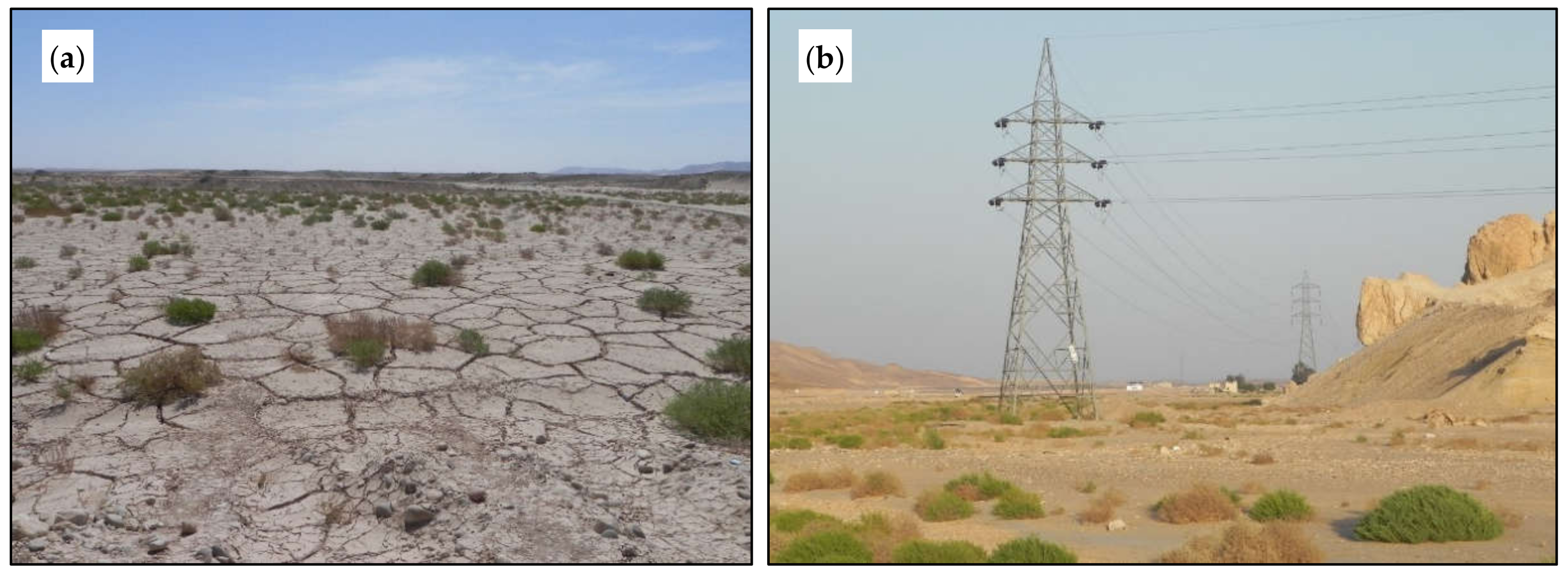
Figure 3.
Simplified outline for the proposed methodology in this research.

Figure 4.
Wadi Qena geomorphometric analysis. The inner basin (15) records the average parameter values of the entire Wadi Qena basin.
Figure 4.
Wadi Qena geomorphometric analysis. The inner basin (15) records the average parameter values of the entire Wadi Qena basin.
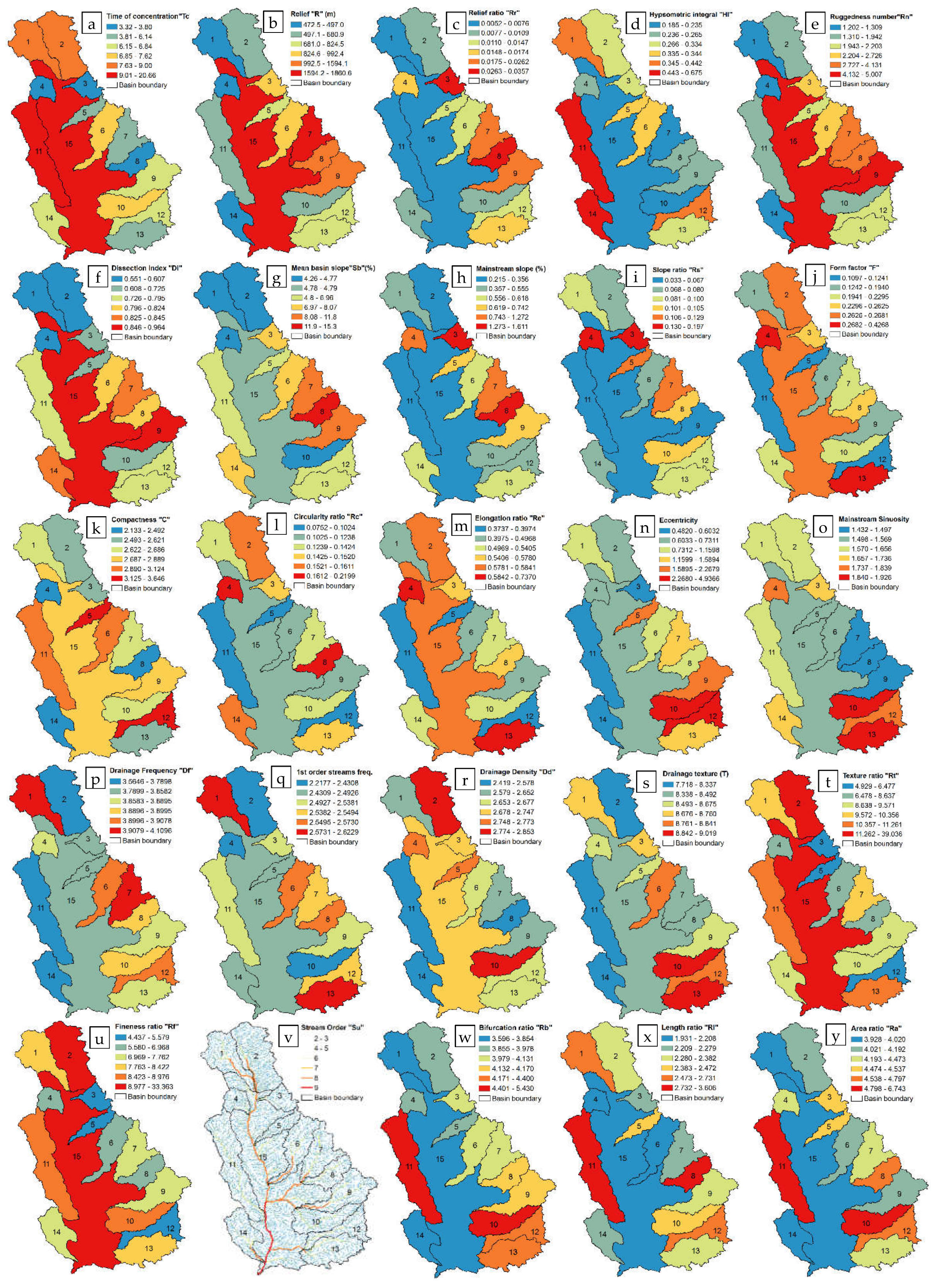
Figure 5.
Correlation matrix between the assessed geomorphologic parameters based on R2 values. This figure indicates that each geomorphologic parameter is best correlated with the other metrics of its same group.
Figure 5.
Correlation matrix between the assessed geomorphologic parameters based on R2 values. This figure indicates that each geomorphologic parameter is best correlated with the other metrics of its same group.
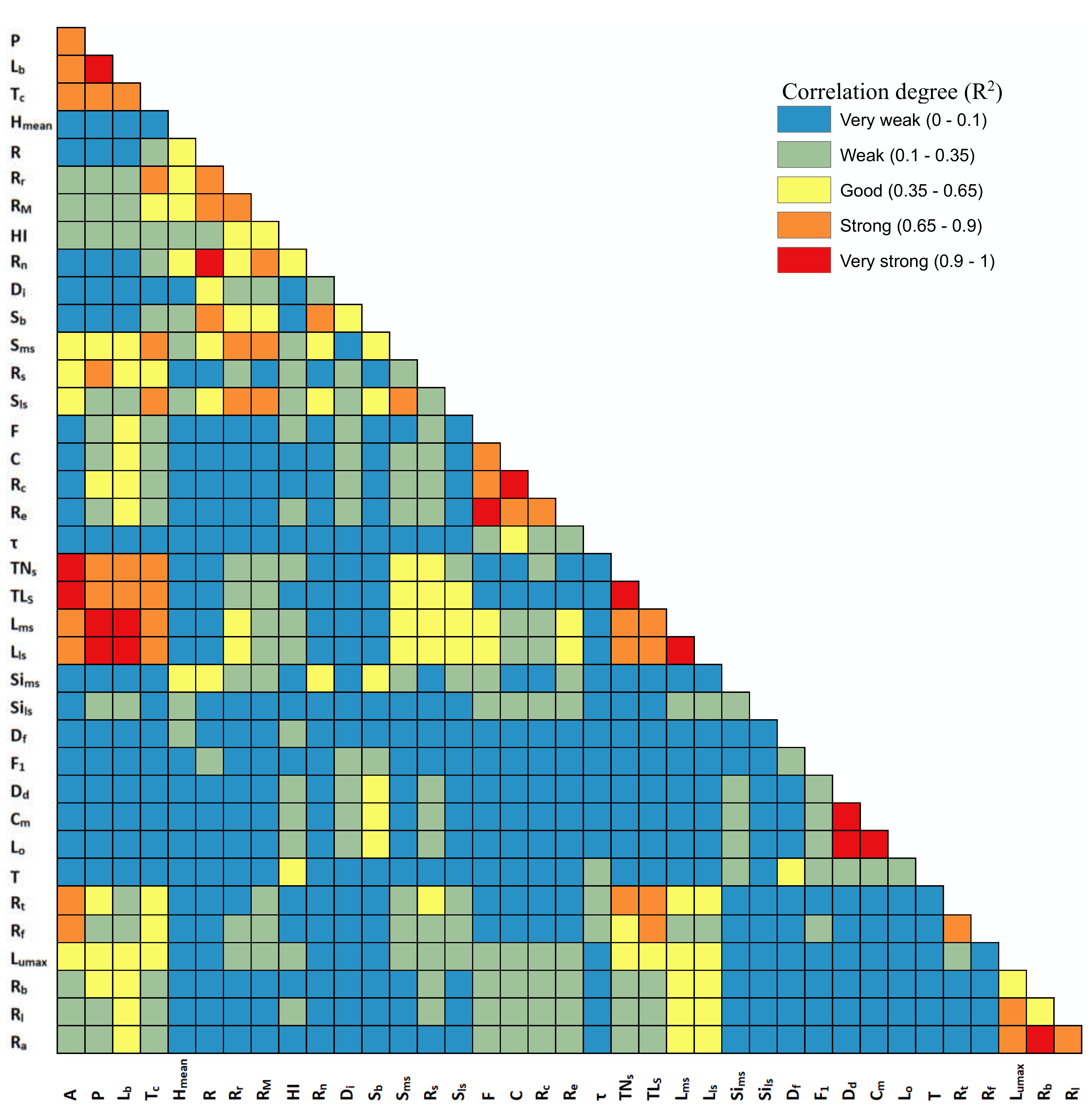
Figure 6.
Comparisons between different SRTM Digital Elevation Model (DEM) data: (a) 30 arc-sec resolution, (b) 3 arc-sec resolution and (c) 1 arc-resolution; the last dataset captures the drainage system better than the lower resolution DEM data, and is thus the preferred choice with which to study the flash floods at Wadi Qena.
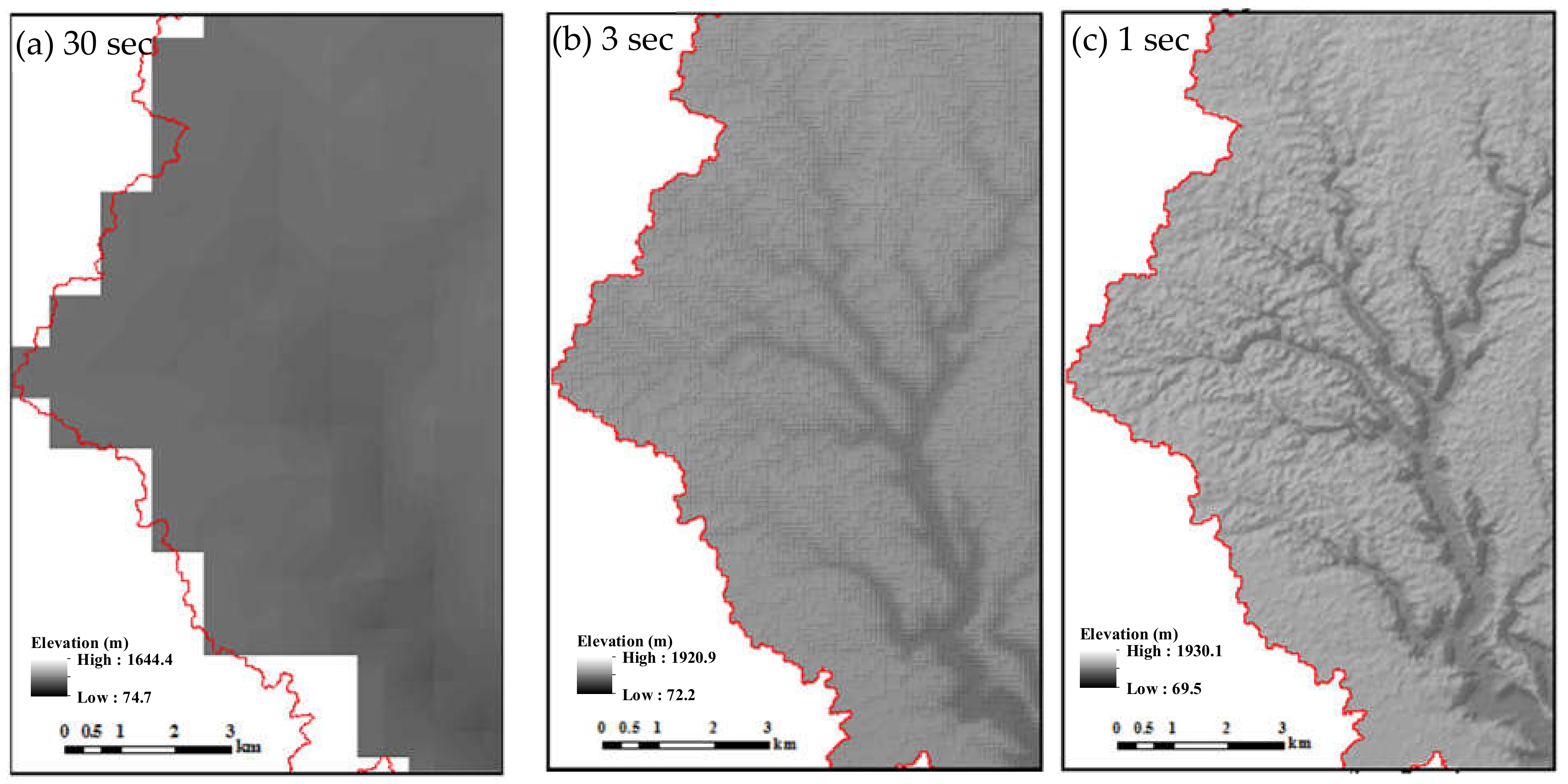
Figure 7.
Hydro-BEAM schematic diagram (after Kojiri et al. [34]). (a) Hydro-BEAM basic structure; (b) surface layer kinematic wave model; (c) simple representation of subsurface storage tank layers.
Figure 7.
Hydro-BEAM schematic diagram (after Kojiri et al. [34]). (a) Hydro-BEAM basic structure; (b) surface layer kinematic wave model; (c) simple representation of subsurface storage tank layers.
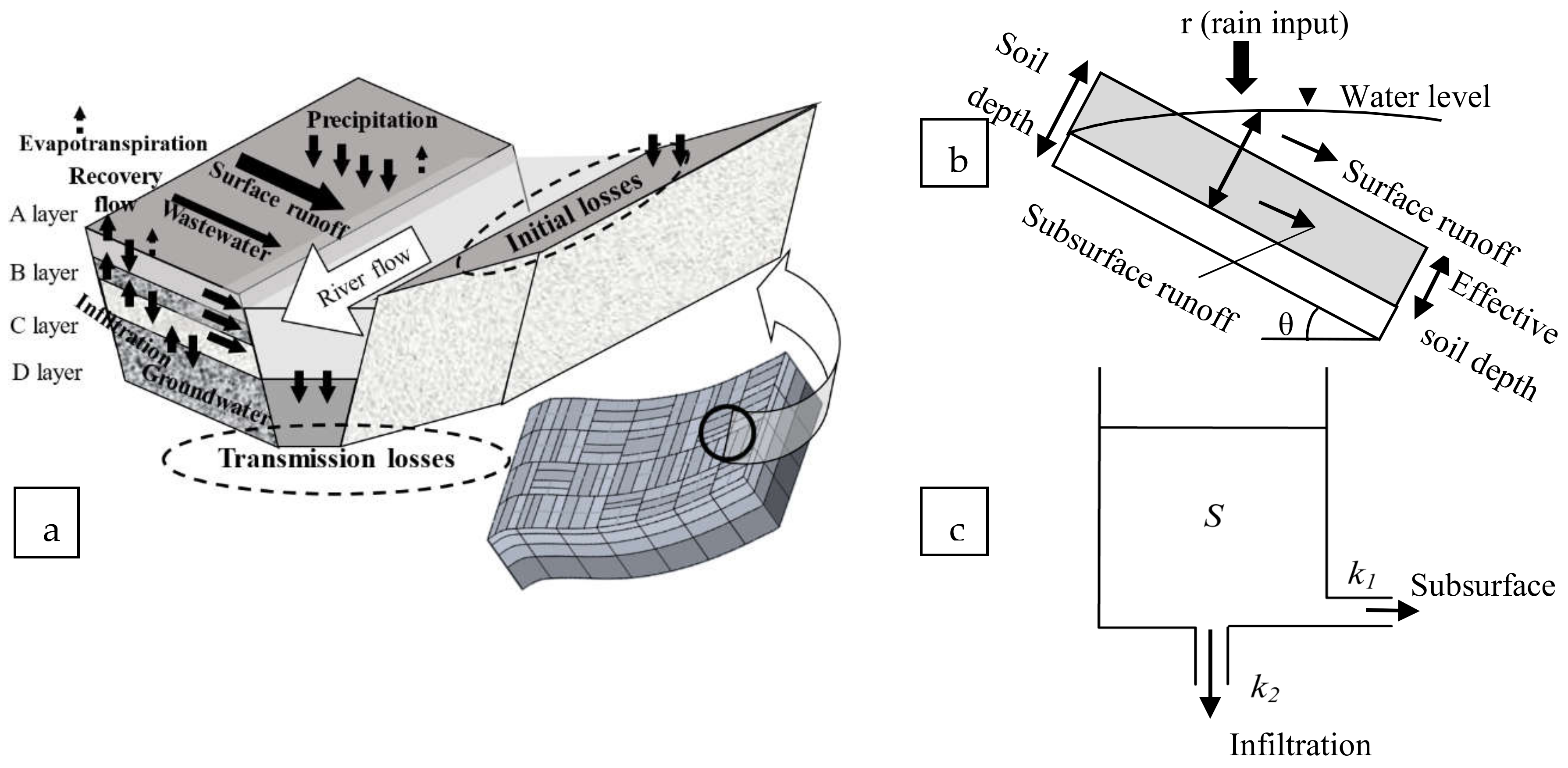
Figure 8.
(a) Wadi Qena watershed and locations where the simulated floods hydrographs are shown; for the (b) November 1994, (c) January 2010, (d) January 2013 and (e) March 2014 flood events.
Figure 8.
(a) Wadi Qena watershed and locations where the simulated floods hydrographs are shown; for the (b) November 1994, (c) January 2010, (d) January 2013 and (e) March 2014 flood events.
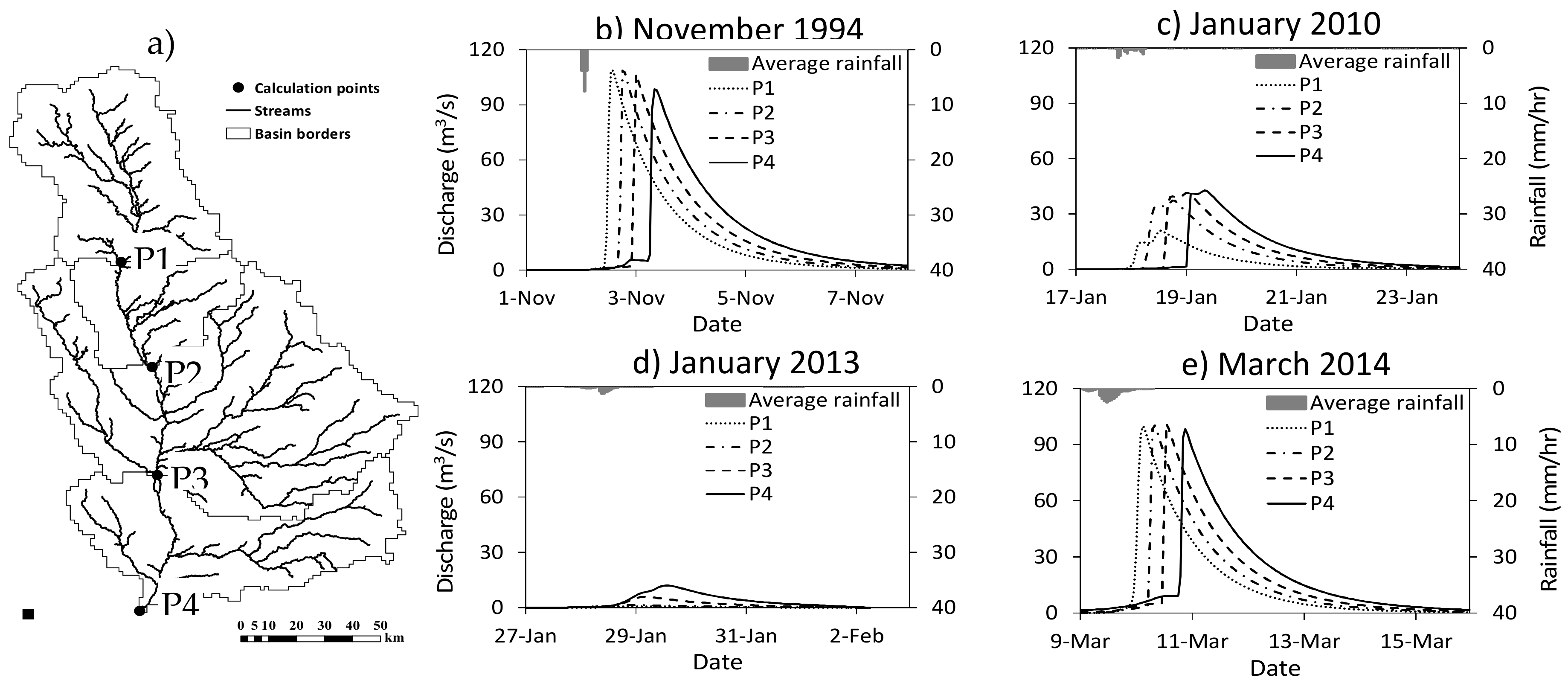
Figure 9.
Geographical distribution maps at Wadi Qena for (1) total rainfall input; (2) simulated peak surface runoff for the (a) November 1994, (b) January 2010, (c) January 2013 and (d) March 2014 flood events. The rainfall data of Nov. 1994 event were used form Geith and Sultan [48] with a resolution of 0.5 degree whereas the GSMaP data of 0.1 degree resolution were used for the other events.
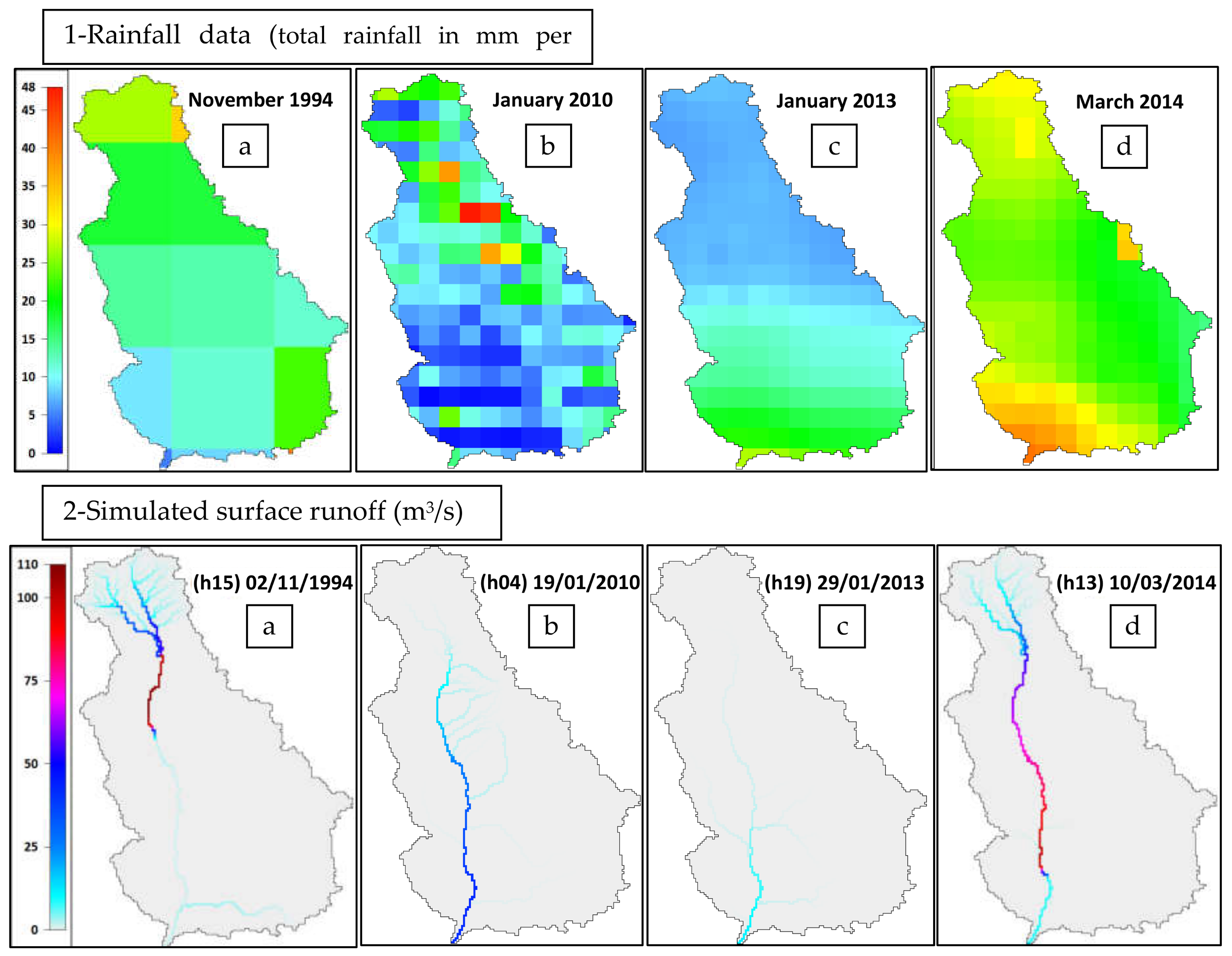
Figure 10.
Simulated hydrographs at the different sub-basins outlets (sub-basin 1–14) and the entire Wadi Qena basin for the nine applied synthetic storm types based on total rainfall amount and duration.
Figure 10.
Simulated hydrographs at the different sub-basins outlets (sub-basin 1–14) and the entire Wadi Qena basin for the nine applied synthetic storm types based on total rainfall amount and duration.
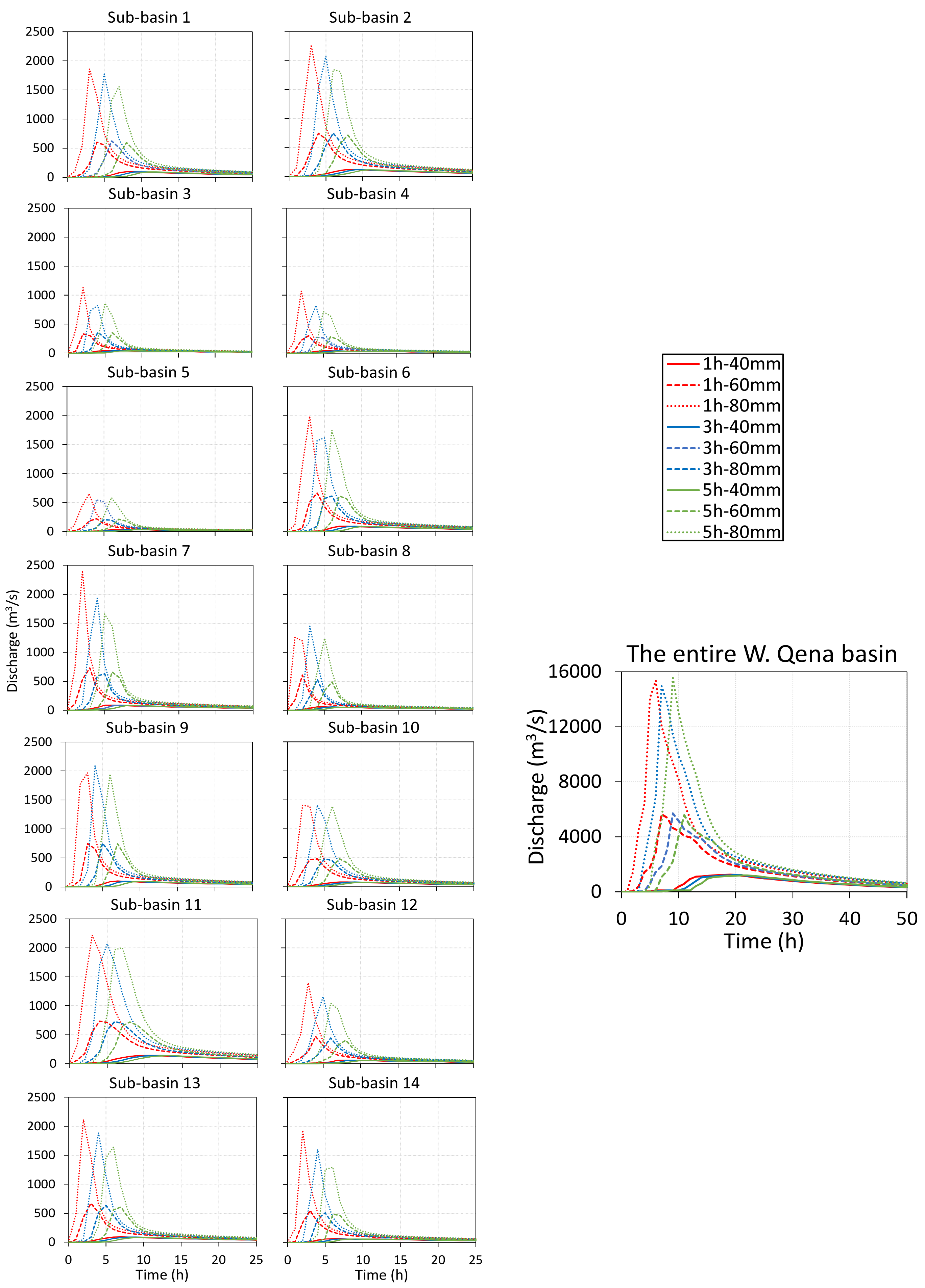
Figure 11.
Relationship between the estimated hydrological indices and basin scale parameters: (a) area (A), (b) basin length (Lb) and (c) time of concentration (Tc) for the different applied storm intensities at all sub-basins.
Figure 11.
Relationship between the estimated hydrological indices and basin scale parameters: (a) area (A), (b) basin length (Lb) and (c) time of concentration (Tc) for the different applied storm intensities at all sub-basins.

Figure 12.
Relationship between the hydrological indices and significant basin topographic parameters: (a) Relief ratio (Rr), (b) Melton relative relief (RM), (c) mean basin slope (Sb), (d) mainstream slope (Sms) and (e) slope ratio (Rs) under different storm intensities.
Figure 12.
Relationship between the hydrological indices and significant basin topographic parameters: (a) Relief ratio (Rr), (b) Melton relative relief (RM), (c) mean basin slope (Sb), (d) mainstream slope (Sms) and (e) slope ratio (Rs) under different storm intensities.

Figure 13.
Relationship between the hydrological indices and some basin shape parameters: (a) form factor (F) and (b) compactness (C) with different storm intensities.
Figure 13.
Relationship between the hydrological indices and some basin shape parameters: (a) form factor (F) and (b) compactness (C) with different storm intensities.

Figure 14.
Relationship between the hydrological indices and significant basin drainage parameters: (a) total stream number (TNS), (b) mainstream length (Lms), (c) texture ratio (Rt) and (d) fineness ratio (Rf) under different storm intensities.
Figure 14.
Relationship between the hydrological indices and significant basin drainage parameters: (a) total stream number (TNS), (b) mainstream length (Lms), (c) texture ratio (Rt) and (d) fineness ratio (Rf) under different storm intensities.
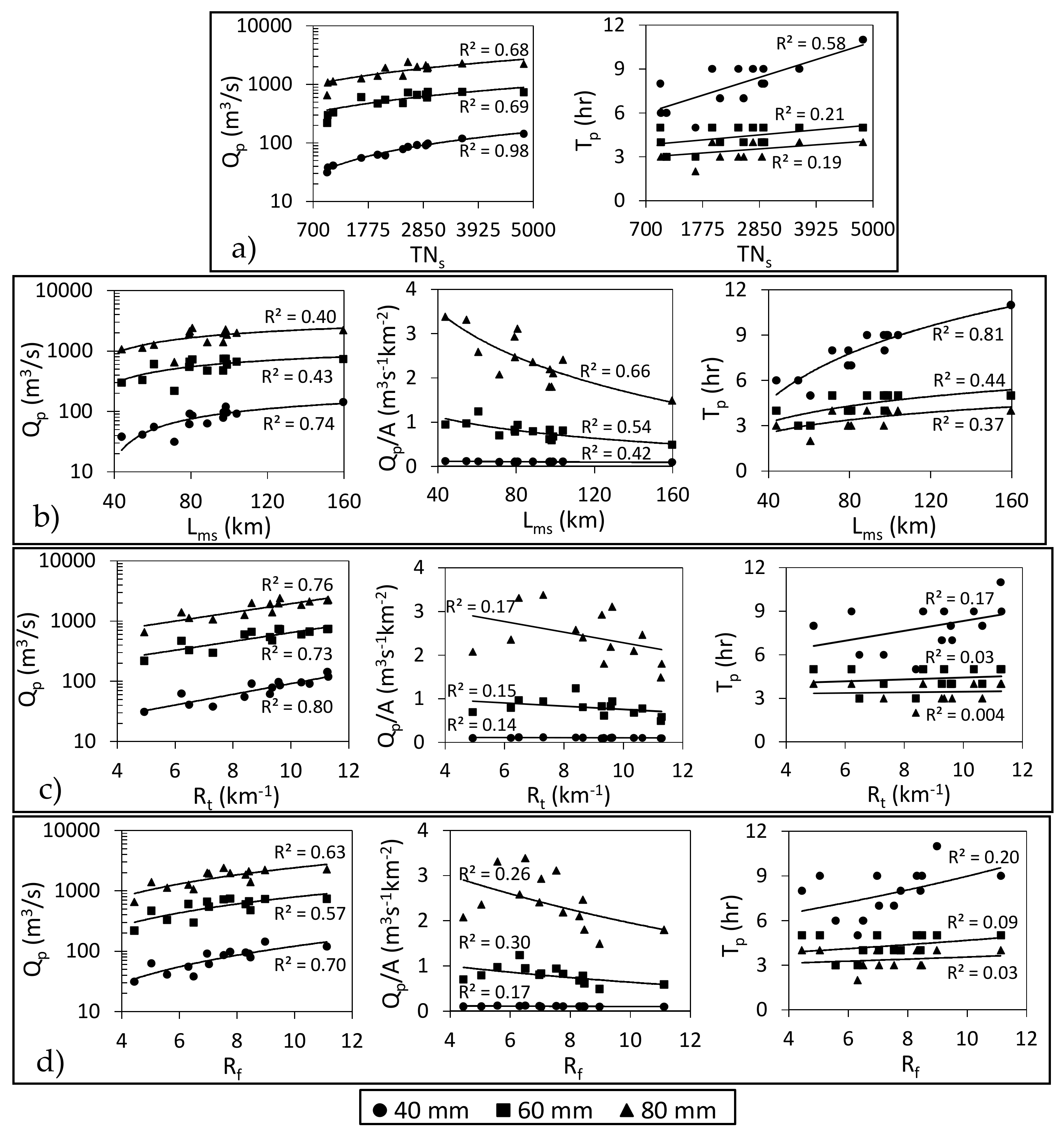
Figure 15.
Correlation between the hydrological indices and drainage network measures based on stream order: (a) maximum order stream length (Lumax), (b) bifurcation ratio (Rb), (c) length ratio (Rl), (d) area ratio (Ra), (e) Rl/Lumax and (f) Rb.Lumax/(Rl.Ra) under different storm intensities.
Figure 15.
Correlation between the hydrological indices and drainage network measures based on stream order: (a) maximum order stream length (Lumax), (b) bifurcation ratio (Rb), (c) length ratio (Rl), (d) area ratio (Ra), (e) Rl/Lumax and (f) Rb.Lumax/(Rl.Ra) under different storm intensities.


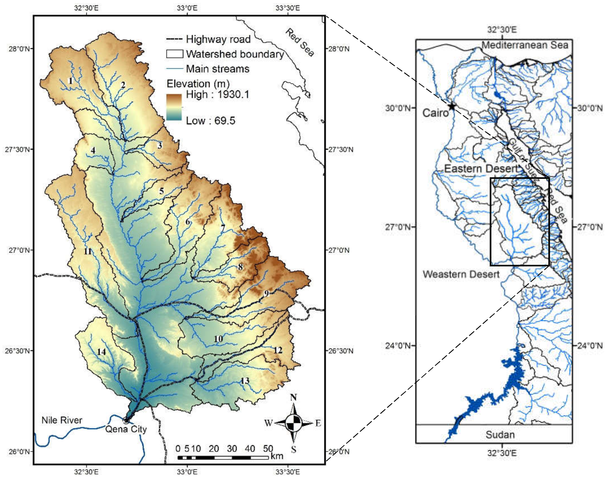
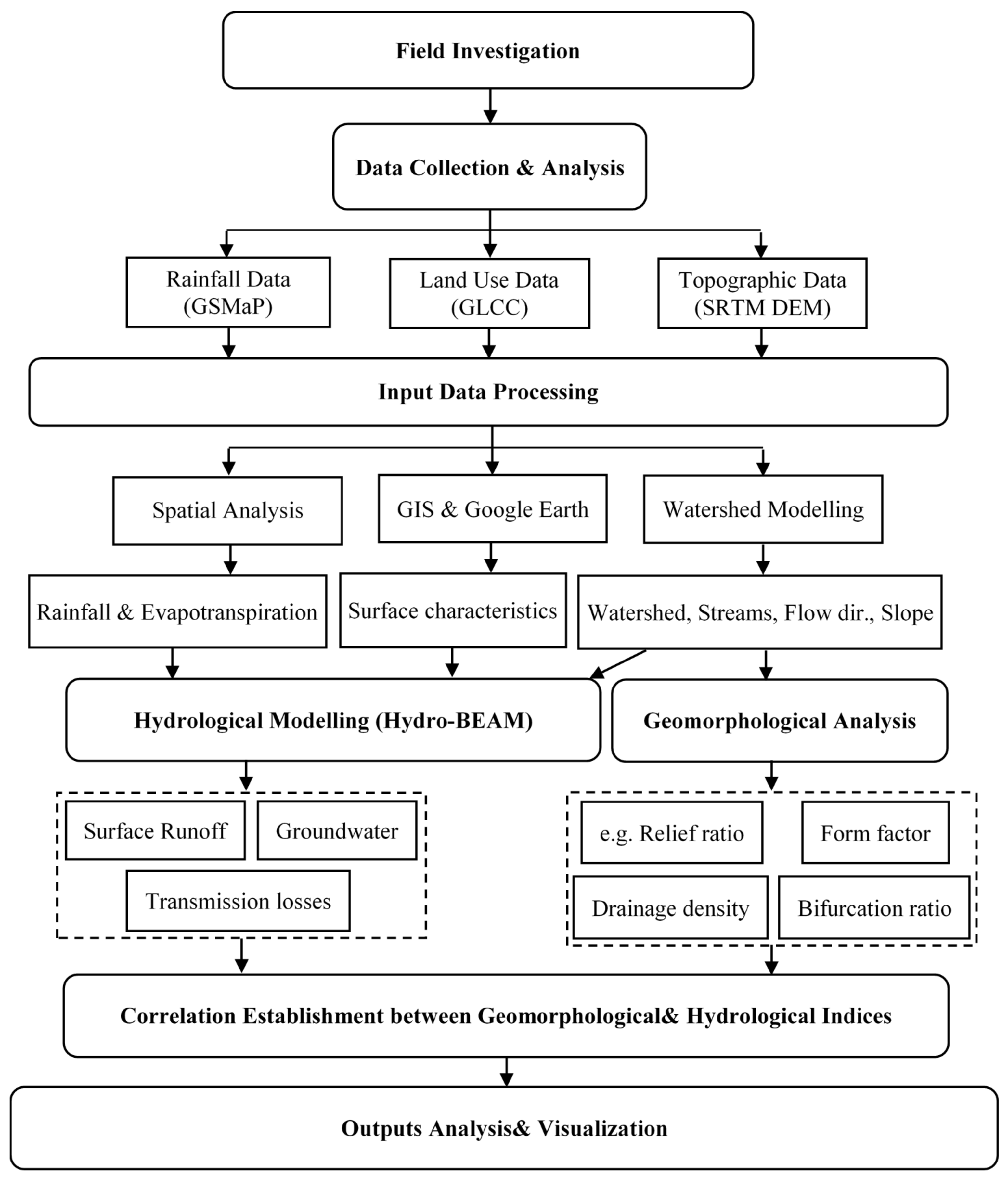
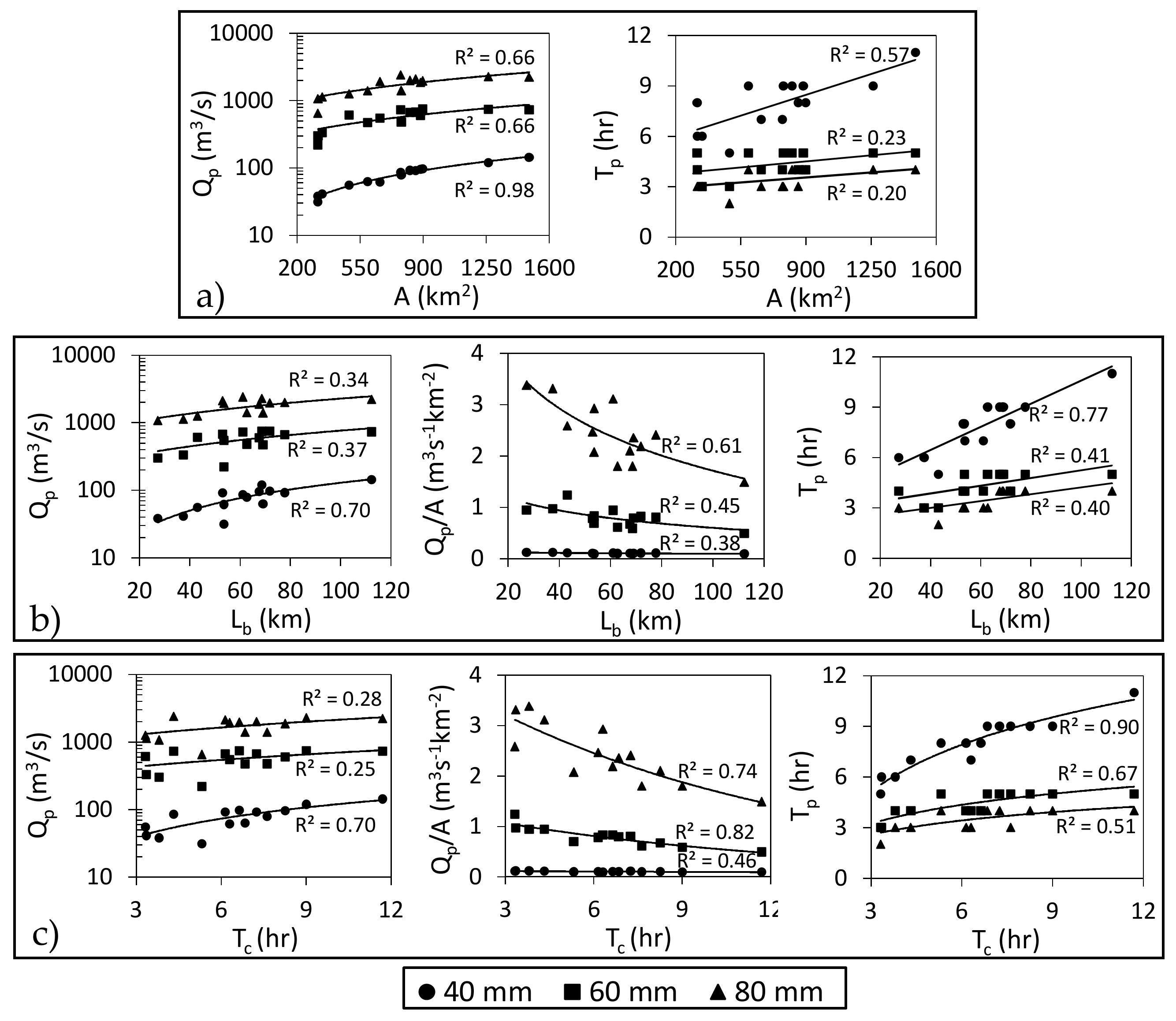
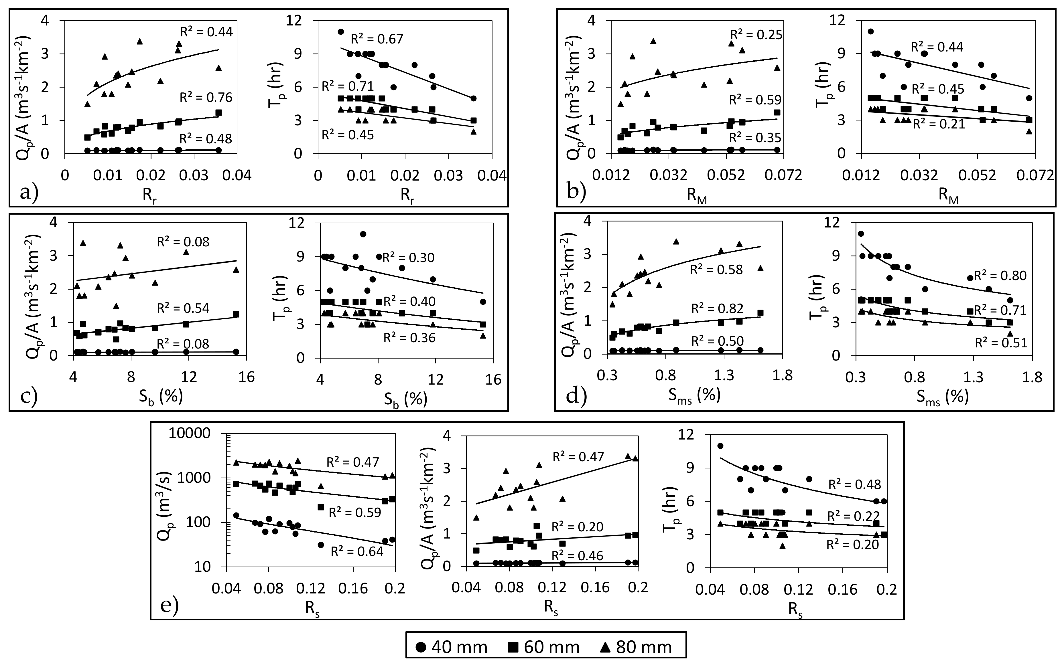
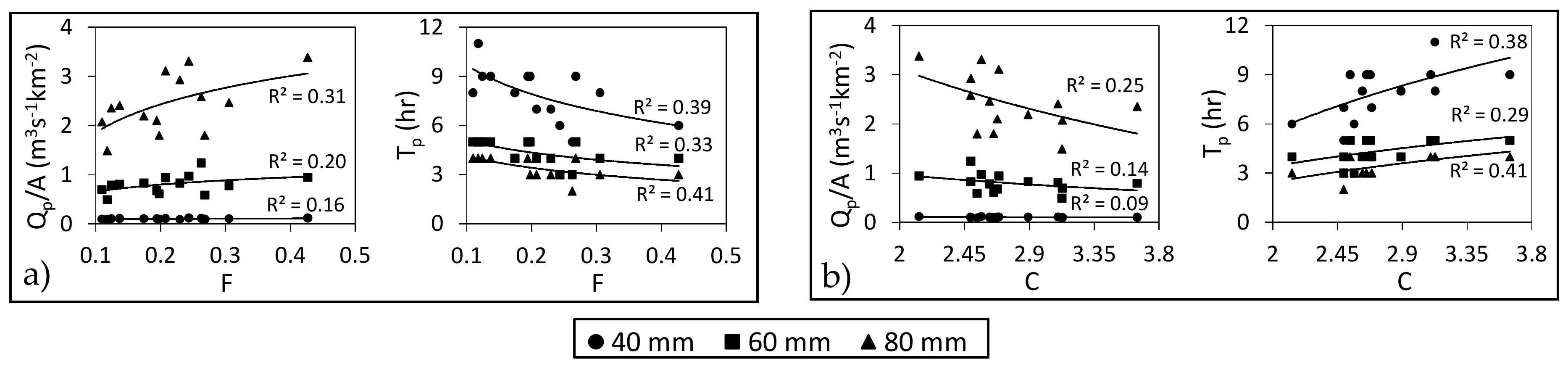
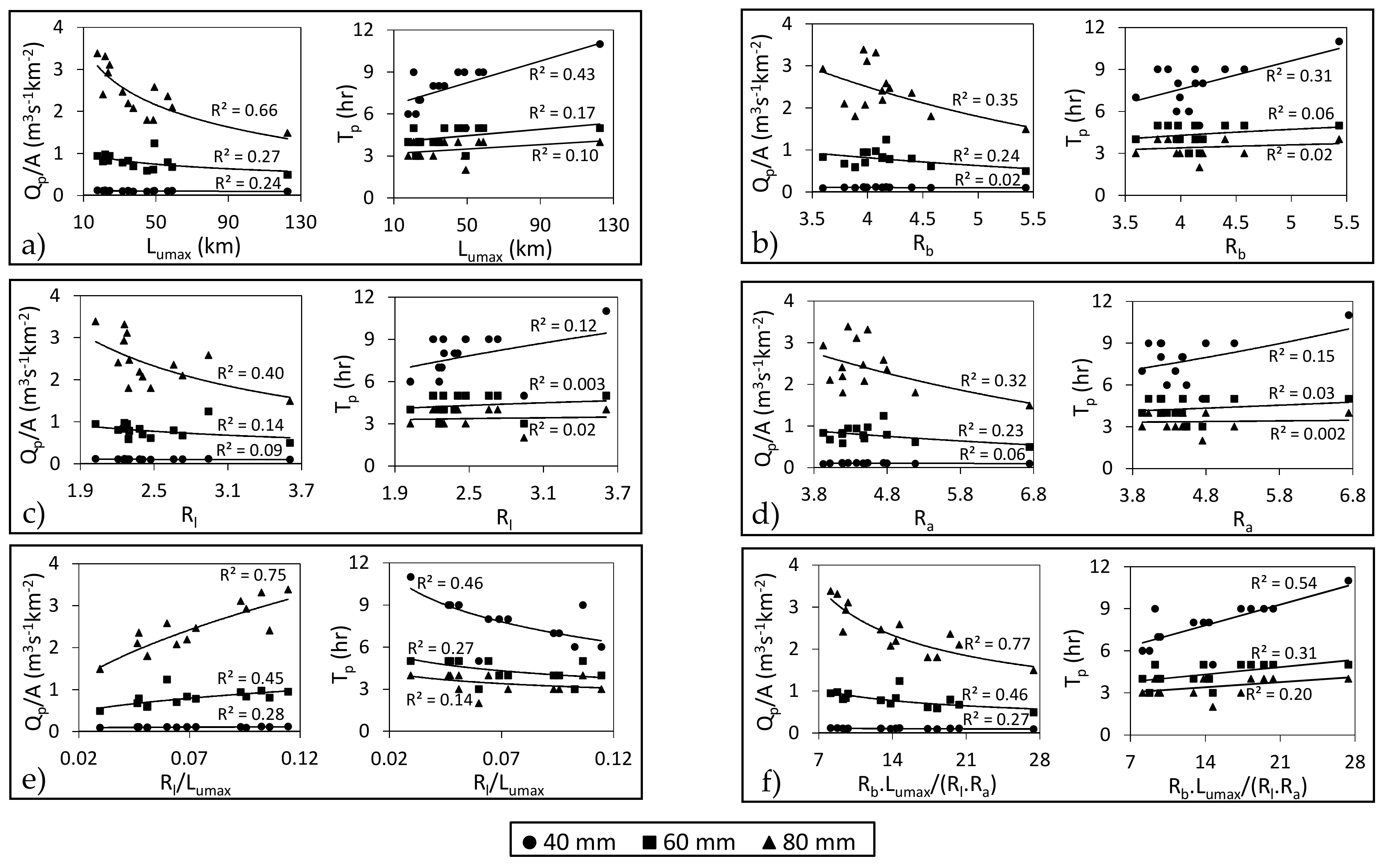
Table 1.
List and description of the used geomorphometric parameters.
| Parameter (Abbreviation) | Unit | Range | SD | Formula | Reference |
|---|---|---|---|---|---|
| Scale metrics | |||||
| Area (A) | km2 | 314.9–1487.9 | 328.7 | Basin area | |
| Perimeter (P) | km | 134.5–427.3 | 72.6 | Basin perimeter | |
| Basin length (Lb) | km | 27.2–112.3 | 19.6 | Basin maximum dimension | |
| Time of concentration (Tc) | h | 3.3–11.7 | 2.26 | [54] | |
| Topographic metrics | |||||
| Mean elevation (Hmean) | m | 426.9–727.4 | 95.9 | Mean basin elevation | |
| Relief (R) | m | 472.5–1601.3 | 391.7 | [55] | |
| Relief ratio (Rr) | - | 0.005–0.036 | 0.0084 | [55] | |
| Melton relative relief (RM) | km−1 | 0.0152–0.07 | 0.0169 | [56] | |
| Hypsometric Integral (HI) | - | 0.185–0.675 | 0.137 | [57] | |
| Ruggedness number (Rn) | - | 1.202–4.228 | [58] | ||
| Dissection index (Di) | 0.54–0.85 | 1.00 | [59] | ||
| Mean basin slope (Sb) | % | 4.3–15.3 | 2.98 | Average basin slope | |
| Mainstream slope (Sms) | % | 0.34–1.61 | 0.39 | Main stream average slope | |
| Slope ratio (Rs) | - | 0.049–0.197 | 0.0414 | [19] | |
| Longest stream slope (Sls) | % | 0.35–1.68 | 0.42 | Longest stream average slope | |
| Shape metrics | |||||
| Form factor (F) | - | 0.11–0.43 | 0.083 | [60] | |
| Compactness (C) | - | 2.13–3.65 | 0.36 | [60] | |
| Circularity ratio (Rc) | - | 0.075–0.22 | 0.034 | [61] | |
| Elongation ratio (Re) | - | 0.374–0.737 | 0.098 | [55] | |
| Eccentricity ( ) | - | 0.48–4.94 | 1.17 | [10] | |
| Drainage network aspects | |||||
| Total stream number (TNs) | - | 970–4812 | 1030.3 | Total stream number | |
| Total streams length (TLs) | km | 873.2–3835.6 | 879.1 | Total stream length | |
| Mainstream length (Lms) | km | 43.8–159.6 | 26.8 | Main stream length | |
| Longest stream length (Lls) | km | 45.1–160.0 | 26.3 | Longest stream length | |
| Main stream sinuosity (Sims) | - | 1.432–1.926 | 0.155 | [62] | |
| Longest stream sinuosity (Sils) | - | 1.509–1.959 | 0.146 | [62] | |
| Drainage frequency (Df) | km−2 | 3.56–4.11 | 0.117 | [63] | |
| 1st order streams frequency (F1) | km−2 | 2.218–2.623 | 0.097 | ||
| Drainage density (Dd) | km−1 | 2.42–2.85 | 0.117 | [60] | |
| Channel maintenance (Cm) | km | 0.351–0.413 | 0.016 | [55] | |
| Overland flow length (Lo) | km | 0.175–0.207 | 0.008 | [63] | |
| Drainage texture (T) | km−1 | 7.72–9.02 | 0.34 | [64] | |
| Texture ratio (Rt) | km−1 | 4.9–11.3 | 1.87 | [64] | |
| Fineness ratio (Rf) | - | 4.4–11.1 | 1.68 | [58] | |
| Stream order (Su) | - | 1–9 | Hierarchical rank | [65] | |
| Main trunk length (Lumax) | km | 17.7–122.7 | 25.9 | Highest stream order length | |
| Bifurcation ratio (Rb) | - | 3.596–5.43 | 0.421 | [60] | |
| Length ratio (Rl) | - | 2.02–3.61 | 0.386 | [60] | |
| Area ratio (Ra) | - | 3.93–6.74 | 0.68 | [60] |
SD: Standard deviation, Hmin: Minimum elevation, Hmax: Maximum elevation, Lc: Distance from basin centroid to its outlet, Wc: Basin width at the centroid.
Table 2.
Summary of target flood events simulated at Wadi Qena.
| Simulation Results | 1994 | 2010 | 2013 | 2014 | 3 h Synthetic Homogenous Storm | ||
|---|---|---|---|---|---|---|---|
| 40 mm | 60 mm | 80 mm | |||||
| Total rain volume (×106 m3) | 237 | 124 | 153 | 393 | 628 | 942 | 1256 |
| Peak discharge (m3/s) | 109.5 | 42.67 | 12.0 | 101.1 | 1230.9 | 5564.6 | 14,964 |
| Total outlet discharge volume (×106 m3) | 10.6 | 5.6 | 1.79 | 10.9 | 139 | 327 | 588 |
| Outlet discharge percent (%) | 4.49 | 4.57 | 1.17 | 2.76 | 22.21 | 34.72 | 46.91 |
| Total transmission losses volume (×106 m3) | 14.6 | 6.9 | 1.4 | 13.8 | 102 | 212 | 328 |
| Total transmission losses percent (%) | 6.16 | 5.47 | 0.92 | 3.52 | 16.27 | 22.0 | 26.22 |
© 2017 by the authors. Licensee MDPI, Basel, Switzerland. This article is an open access article distributed under the terms and conditions of the Creative Commons Attribution (CC BY) license (http://creativecommons.org/licenses/by/4.0/).
Share and Cite
MDPI and ACS Style
Abdel-Fattah, M.; Saber, M.; Kantoush, S.A.; Khalil, M.F.; Sumi, T.; Sefelnasr, A.M. A Hydrological and Geomorphometric Approach to Understanding the Generation of Wadi Flash Floods. Water 2017, 9, 553. https://doi.org/10.3390/w9070553
AMA Style
Abdel-Fattah M, Saber M, Kantoush SA, Khalil MF, Sumi T, Sefelnasr AM. A Hydrological and Geomorphometric Approach to Understanding the Generation of Wadi Flash Floods. Water. 2017; 9(7):553. https://doi.org/10.3390/w9070553
Chicago/Turabian StyleAbdel-Fattah, Mohammed, Mohamed Saber, Sameh A. Kantoush, Mohamed F. Khalil, Tetsuya Sumi, and Ahmed M. Sefelnasr. 2017. "A Hydrological and Geomorphometric Approach to Understanding the Generation of Wadi Flash Floods" Water 9, no. 7: 553. https://doi.org/10.3390/w9070553
Note that from the first issue of 2016, this journal uses article numbers instead of page numbers. See further details here.