Article

Optimal Hedging Rules for Water Supply Reservoir Operations under Forecast Uncertainty and Conditional Value-at-Risk Criterion

1
College of Hydrology and Water Resources, Hohai University, NO. 1, Xikang Road, Nanjing 210098, China
2
Nanjing Hydraulic Research Institute, No. 223, Guangzhou Road, Nanjing 210029, China
3
National Engineering Research Center of Water Resources Efficient Utilization and Engineering Safety, Hohai University, NO. 1, Xikang Road, Nanjing 210098, China
4
Power China Zhongnan Engineering Corporation Limited, NO. 16, East Xiangzhang Road, Changsha 410014, China
5
State Key Laboratory of Hydrology-Water Resources and Hydraulic Engineering, Hohai University, NO. 1, Xikang Road, Nanjing 210098, China
*
Author to whom correspondence should be addressed.
Water 2017, 9(8), 568; https://doi.org/10.3390/w9080568
Submission received: 1 May 2017 / Revised: 4 July 2017 / Accepted: 26 July 2017 / Published: 30 July 2017

Abstract

:
Hedging rules for water supply reservoir operations provide guidelines for balancing the consequences of competing water allocations. When inflow forecast uncertainty is addressed, hedging acts as insurances for offsetting the negative influence of water shortage in the future, especially when drought is anticipated. This study used a risk-averse criterion, the conditional value-at-risk (CVaR), rather than the expected value (EV) criterion, to rationalize water delivery for overcoming the shortcomings of risk-neutral hedging rules in minimizing water shortage impacts in unfavorable realizations, in which actual inflow is less than anticipated. A two-period hedging model with the objective of maximizing the CVaR of total benefits from water delivery and water storage is established, and the optimal hedging rules using first-order optimality condition are analytically derived. Differences in hedging rules under the two criteria are highlighted by theoretical analysis and numerical experiments. The methods are applied to guide the operations of a water supply reservoir, and results show that: (1) the hedging rules under the EV criterion are special cases under the CVaR criterion; (2) water delivery in the current period would be greatly curtailed under the high influence of forecast uncertainty or the significant risk-averse attitude of decision makers; (3) hedging to maximize the CVaR of total benefit is at the cost of reducing the EV of total benefit; and (4) in real-time operations, compared with the hedging policies under the EV criterion, the hedging policies under the CVaR criterion would be more effective when applied to dry and extremely dry hydrological conditions, especially when inflow is overestimated. These implications provide new insights into rationing water supply and risk aversion.

1. Introduction

Modern water resource systems face water shortage risks from multiple uncertainties, which could cause negative social, economic, and ecological impacts. To alleviate the negative impacts of water shortage, management techniques such as increasing water supply and decreasing water demand are essential for the supply–demand balance. As a common component of a water resources system, reservoirs [1,2] can redistribute natural water resources over time by using water storage. However, during drought, total water availability may be insufficient to meet total demand, resulting in conflicts among competing water uses in different periods. In such cases, whether limited water is delivered for immediate use or kept for future use should be decided to best balance the consequences of current water use versus those in the future. For water supply reservoir, the consequence means that both the benefits of the current water delivery and carryover storage (for future water deliveries) can be jointly assessed. When potential drought is anticipated, the water delivery in the current period can be curtailed to alleviate the negative influence of water shortage in the future [3], although the current availability is adequate to satisfy immediate water demand. This condition is a hedging policy [4,5], which is a water-saving approach to reducing maximum drought impacts.
Early studies have focused on developing various forms of hedging policies [6] or models for reservoir operations. Hashimoto et al. [7] analyzed the formulation of loss function and its corresponding optimal operational rules. Klemes [8] verified that the standard operating policy (SOP) is the best policy given a linear loss function. For nonlinear loss or benefit functions, hedging rules vary with regard to various model formulations and purposes. Draper and Lund [3] introduced a two-stage optimal hedging model that determines the optimal water delivery strategy for maximizing the summation of current and future benefits, and they found that the optimality condition for hedging is at which the marginal benefit of storage equals the marginal benefit of water release. They then derived the analytic hedging rules for monotonic increasing benefit functions. Shiau [9] noted that either the release or the storage deviating from their targets could cause economic loss and used normalized deviations as loss functions to characterize competing water allocations. Zeng et al. [10] extended the study of Draper and Lund [3] to explore optimal hedging rules for multiple reservoirs that operate in parallel with a joint water demand.
Decision makers often rely on inflow forecasts [11] to estimate potential water available for allocations, considering that water supply reservoir operations usually require scheduling releases and storage over several months. The influence of inflow forecast uncertainty should be incorporated into decision making, given that it is often difficult to precisely forecast the actual inflow at the beginning of the current time. Therefore, the hedging model turns out to be a stochastic optimization problem wherein the conventional objective [12,13] is to optimize the expected value (EV) of total benefit or total loss. This model yields a risk-neutral decision that is suited for all possible future inflow realizations, considering both cases wherein inflow is overestimated or underestimated. You and Cai [14] examined how reservoir inflow uncertainty affects hedging operations using the EV of total benefit as the objective. They concluded that hedging should reduce the current release to face future risk induced by hydrological uncertainty. Zhao et al. [15] developed optimal hedging rules for reservoir flood operations considering the influence of forecast uncertainty. To minimize the total expected flood damages, they analyzed how the expected flood-safety margin should be optimally allocated to the current and future time periods for different levels of flood events.
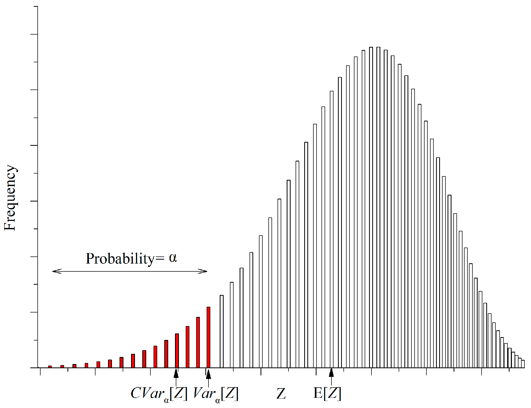
The expected value (EV) criterion provides a risk-neutral policy that is indifferent between gaining benefit in favorable realizations and suffering loss in unfavorable realizations because it seeks the best average outcome. Consequently, high benefit can be obtained when inflow is high, whereas high loss could also be a result of a low inflow. The optimal policy yielded from the EV criterion is often vulnerable to risks in unfavorable realizations. In water resource allocations, decision makers are often more concerned about the overall benefit in unfavorable realizations wherein water is less than anticipated [16,17]. This concern suggests a more conservative criterion, rather than EV, to focus on outcomes under unfavorable or even worst-case scenarios. The conditional value-at-risk (CVaR), or the expected shortfall, is a suitable criterion for assessing the mean value of outcome from undesirable cases, which is originally used in finance [18,19] to measure expected losses above a given loss threshold. Yamout et al. [20] verified that applying the CVaR criterion to water allocation problems presents continuous and consistent model behavior compared with the modeling results under the value-at-risk (VaR) criterion. Piantadosi et al. [21] proposed a model for managing the urban storm water to minimize CVaR, and they showed that the optimal policy under CVaR differs from the optimal policy obtained under expected loss minimization criterion. Hu et al. [22] established a multiobjective model including water allocation equality and economic efficiency risk control, and the model incorporates a constraint to bind the CVaR of economic efficiency risk induced by the uncertainty of water availability. The optimal decision and model performance under the CVaR criterion differ from that under the expectation criterion. Thus, analytic derivations and analysis on the related formulations of hedging rules could provide decision makers intuitive and effective guidance in rationing water resource allocations.
The purposes of this study are: (1) to derive the hedging rules for water supply reservoir operations under the CVaR criterion considering inflow forecast uncertainty and (2) to explore the differences in rationing water deliveries and related performances under two criteria (CVaR and EV). Specifically, this study extends the studies of Draper and Lund [3] and You and Cai [14] and establishes a stochastic programming model for hedging under the consideration of inflow forecast uncertainty. Setting the objectives of maximizing the EV and the CVaR of total benefit, we derive the optimality condition of hedging policies and their analytic formulations. Comparative experiments and model simulations are conducted to investigate the differences. The methods are derived under the background of a reservoir solely for water supply, and the utility of water supply and water storage are evaluated in monetary values. These methods could limit the application of the methodologies to the operations of multipurpose reservoirs, except for the cases wherein the utility of operational purposes can be common-measured or converted into the same measuring unit using weights or conversion factors.
The remainder of this paper is organized as follows. Section 2 reviews the classical two-period optimal hedging model under the EV criterion and extends it to a hedging model using the CVaR criterion. Thereafter, we derive the optimality condition for the hedging model under the CVaR criterion and obtain analytically formulated hedging rules. Section 3 applies the methodology to a water supply reservoir, the Foziling Reservoir in China, and investigates the influences of parameters on the hedging rules and their statistical measures via sensitivity analysis. Section 4 discusses the differences in performances of hedging rules when applied to guide real-time operations using numerical simulations. Finally, Section 5 concludes the study.

2. Materials and Methods

2.1. Model Formulation

2.1.1. Two-Period Optimal Hedging Model under the EV Criterion

The classical two-period optimal hedging model, which is established for a water supply reservoir, seeks the optimal solution of water delivery that resolves the conflict between immediate and future water use. Specifically, Draper and Lund [3] used a benefit function B ( ) to assess the current benefit associated with water delivery D and a carryover storage value function C ( ) to calculate the future benefit related to carryover storage S . B ( ) and C ( ) can be measured in terms of monetary values or utilities for the reservoir. These two functions are assumed to be monotonically increasing and concave. The model formulation is provided as follows:
max D   E [ Z ] = E [ B ( D ) + C ( S ) ] = B ( D ) + E [ C ( S ) ]
where Z is the total benefit measured by monetary value assessed by Chinese Yuan, (CNY); E [ ] is the EV function; and E [ Z ] is the EV of the total benefit, (CNY).
The following constraints are addressed:
E [ S ] + D = A
A = S 0 + I E P
0 S k
0 D d m
where A is the water available for allocation, which equals the summation of storage volume at the beginning of current time period ( S 0 ) and the EV of inflow volume ( I ) during the current period subtracting the EV of evaporation ( E P ), (m3); k is the storage capacity of the reservoir, (m3); and d m is the user demand, (m3).
For the given functions of B ( D ) and C ( S ) , the optimal solution of water delivery ( D ) can be obtained. D could be less than dm such that a certain amount of water is kept for future use, even when the water available can meet the current user demand. This strategy saves some water from current use to hedge against the negative influence of future water shortage induced by streamflow uncertainty.
The model provides the optimal hedging policy under the EV criterion considering streamflow uncertainty. However, the model exhibits two limitations when applied to guide real-time decision making. First, the model does not explicitly explore the use of streamflow forecasts because it only uses the EV of the current inflow to address uncertainty. In real-time applications, the estimation of the current inflow highly depends on the technologies of inflow forecasts, and the accuracy of inflow forecasts directly affects hedging decisions. Second, the expectation criterion can only provide a risk-neutral solution that suits all possible outcomes of streamflow realizations. When hedging is necessary for water delivery, decision makers often hold a risk-averse attitude and concern about the benefit that can be obtained under unfavorable situations.

2.1.2. Two-Period Optimal Hedging Model under the CVaR Criterion and Forecast Uncertainty

High risk is positively correlated with high returns and losses; as a risk-neutral criterion, which is indifferent with high returns and losses, the EV criterion fails to control the risk of loss. For risk-averse decision makers who expect to decrease the risk of high losses, the EV criterion could be inappropriate for rationing water supply decisions. Therefore, a more conservative index, rather than the EV, should be employed to manage the risk of loss.
The CVaR [18,21] is such a criterion, which assesses the mean value of loss above the threshold V a R under the given confidence level of α . For a specific loss function ( L = f ( X , Y ) ) related to a decision variable X and a random variable Y , C V a R α [ L ] can be characterized as follows:
C V a R α [ L ] = E { L | L V a R α [ L ] }
V a R α [ L ] = min { L | P ( L ) α }
where P ( ) is the cumulative probability function of L ; α is the confidence level ( α [ 0 , 1 ] ); and V a R α [ L ] is the VaR that evaluates the minimum loss such that the probability of exceeding the loss at 1 α .
We use the concept of CVaR to assess the mean value of total benefit below its VaR. The benefit function, rather than the loss function, is used in this study. Thus, the definition of CVaR is changed as follows:
C V a R α [ Z ] = E { Z | Z V a R α [ Z ] } = 1 α V a R α [ Z ] Z g ( Z ) d Z
where g ( Z ) is the probability density function of Z .
The above equations imply that the EV criterion is a special case of the C V a R criterion for α = 1 . Compared with the EV criterion, variations in α allow the C V a R index to measure varied benefit outcomes in the left tail of the benefit distribution. For instance, maximizing C V a R α [ Z ] when α = 0 is equivalent to maximizing the minimum total benefit under the worst case. The relationship among E [ Z ] , V a R α [ Z ] , and C V a R α [ Z ] is shown in Figure 1.
To maximize the total benefit under unfavorable situations, a modified two-period optimal hedging model is established with the objective of maximizing the CVaR of the total benefit:
max D   C V a R α [ Z ] = C V a R α [ B ( D ) + C ( S ) ] = B ( D ) + C V a R α [ C ( S ) ]
Aside from the storage capacity constraint (Equation (4)) and the delivery limit constraint (Equation (5)), the water balance constraints (Equations (2) and (3)) in the model introduced in Section 2.1.1 are modified in this model to consider inflow forecast uncertainty:
S + D = A f + ε
A f = S 0 + I f E P
where A f is the forecasted available water (m3); ε is the forecasting error that obeys the normal distribution such that ε N ( μ , σ 2 ) , and it is the difference between actual inflow and forecasted inflow, ε = I I f (m3); and μ and σ are the mean value and the standard deviation of the forecasting error, (m3), respectively. The forecasted inflow is usually reasonable to be assumed unbiased such that μ = 0 ; otherwise, the system error of forecasted inflow can be corrected by subtracting the mean value μ .
Equations (10) and (11) state that decision makers use forecasted inflow ( I f ) to estimate the water available in real-time decision making, and the uncertainty comes from the forecasting error. Forecasting error ( ε ) directly influences carryover storage ( S ). Thus, the uncertainty of inflow forecasts propagates to S and carryover storage value C ( S ) .

2.2. Optimality Condition and Analytic Solutions

2.2.1. Optimality Condition

With the given values of parameters ( α and σ ) and variables ( S 0 and I f ), Equation (10) implies that the random variable S also obeys the normal distribution with a mean value of A f D and standard deviation of σ ,
S = A f D + ε E [ S ] = A f D σ 2 [ S ] = σ 2
By substituting S using Equation (12) into Equation (9), we can express the objective as a function of D as follows:
max D   C V a R α [ Z ( D ) ] = B ( D ) + C V a R α [ C ( A f D + ε ) ]
F ( D ) is defined as the objective function, and the definition of CVaR is expressed in Equation (8). Equation (13) can then be further expanded as:
max D   F ( D ) = B ( D ) + C V a R α [ C ( A f D + ε ) ] = B ( D ) + 1 α V a R α [ ε ] C ( A f D + ε ) p ( ε ) d ε
where p ( ε ) is the probability density function of ε as given by: p ( ε ) = 1 2 π σ e ε 2 2 σ 2 ( μ = 0 ).
When the storage capacity constraint (Equation (4)) and the delivery limit constraint (Equation (5)) are not binding on the value of D , the optimal D for the objective can be obtained by applying the first-order optimality condition as follows:
F ( D ) D = d B ( D ) d D + 1 α V a R α [ ε ] C ( A f D + ε ) p ( ε ) d ε D = 0
The use of Taylor’s series to expand C ( A f D + ε ) in terms of ε and the neglect of high order terms give the following approximation:
C ( A f D + ε ) C ( A f D ) + C ( A f D ) ε + C ( A f D ) 2 ε 2
C ( A f D + ε ) is substituted back to Equation (15), and then the first-order optimality condition can be derived (Appendix A) as
d B ( D ) d D = C ( A f D ) D + C V a R α [ ε ] C ( A f D ) + C V a R α [ ε 2 ] C ( A f D ) 2
where C V a R α [ ε ] and C V a R α [ ε 2 ] are the CVaR of the random variable ε and that of ε 2 , respectively, which can be characterized as follows:
C V a R α [ ε ] = { μ σ / ( 2 π α ) e V a R α 2 [ ε ¯ ] 2 ,   μ 0 σ / ( 2 π α ) e V a R α 2 [ ε ¯ ] 2 ,   μ = 0
C V a R α [ ε 2 ] = { σ 2 + μ 2 1 α [ σ 2 V a R α [ ε ¯ ] + 2 σ μ 2 π e V a R α 2 [ ε ¯ ] 2 ] ,   μ 0 σ 2 { 1 1 α [ V a R α [ ε ¯ ] 2 π e V a R α 2 [ ε ¯ ] 2 ] } ,   μ = 0
where ε ¯ obeys the standard normal distribution, ε ¯ ~ N ( 0 , 1 ) .

2.2.2. Implications from the Optimality Condition

Defining S f = A f D , we can rewrite the first term in the right hand side of Equation (17) as follows: C ( A f D ) D = C ( A f D ) ( A f D ) ( A f D ) D = d C ( S f ) d S f , which is the marginal benefit of storage. Therefore, Equation (17) indicates that the optimal water delivery ( D ) is derived when the marginal benefit of water delivery equals the summation of marginal benefit of storage and two added terms. To facilitate discussions on the difference of optimal water delivery under the EV and CVaR criteria, we let Δ 1 = C V a R α [ ε ] C ( A f D ) and Δ 2 = C V a R α [ ε 2 ] C ( A f D ) 2 . The value of D is highly influenced by the value of Δ 1 + Δ 2 .
Under the EV criterion, for α = 1 and C V a R 1 [ ε ] = 0 , as well as C V a R 1 [ ε 2 ] = σ 2 , Δ 1 | α = 1 + Δ 2 | α = 1 = C V a R 1 [ ε ] C ( A f D ) + C V a R 1 [ ε 2 ] C ( A f D ) 2 = 0 + σ 2 C ( A f D ) 2 . Under the CVaR criterion, given α < 1 , Δ 1 | α < 1 + Δ 2 | α < 1 = C V a R α [ ε ] C ( A f D ) + C V a R α [ ε 2 ] C ( A f D ) 2 . The difference between the results under the two criteria Δ = ( Δ 1 | α < 1 + Δ 2 | α < 1 ) ( Δ 1 | α = 1 + Δ 2 | α = 1 ) would be calculated as follows, using Equations (18) and (19):
Δ = σ α 2 π e V a R α 2 [ ε ¯ ] 2 [ C ( A f D ) + V a R α [ ε ¯ ] σ C ( A f D ) 2 ]
Equation (20) implies that Δ is strictly nonnegative when α 0.5 for the following reasons: (1) σ α 2 π e V a r α 2 [ ε ¯ ] 2 is negative; (2) C ( A f D ) 0 for a concave storage value function with diminishing marginal storage value; (3) V a r α [ ε ¯ ] is nonpositive for α 0.5 ; and (4) following the assumption made by [14,23], the marginal storage value function is convex in considering precautionary water-saving motive for hedging against future risk. Therefore, the third derivative of storage value function is nonnegative: C ( A f D ) 0 .
Figure 2 plots the equilibriums between the marginal benefits of water delivery and storage under the two criteria. The equilibrium point between the two marginal benefit curves under the expectation criterion is A, and this point would be B under the CVaR criterion with α 0.5 . Accordingly, the optimal water delivery would be further curtailed for α 0.5 ( D α 0.5 ) compared with the optimal water delivery for α = 1 ( D α = 1 ). Consistent with the observations made by You and Cai [14], the forecast uncertainty and precautionary water-saving motive would suggest an increased marginal future utility, especially when decision makers decide to hedge against unfavorable situations wherein the confidence level is below 0.5: α 0.5 .
Consequently, the current water delivery is reduced by ( D α = 1 D α 0.5 ). The reduced release helps increase the water storage S such that the risk of water shortage induced by overestimation of inflow is decreased.
The level of reduced delivery ( D α = 1 D α 0.5 ) is jointly determined by σ and α . Δ 1 + Δ 2 is an increasing function of σ but a decreasing function of α . Thus, D α = 1 D α 0.5 would increase as σ increases or α decreases, which means that water delivery would be greatly curtailed if σ is high or α is low.

2.2.3. Analytic Solutions of Hedging

The examples introduced by Draper and Lund [3] are used, and the analytic hedging solutions can be calculated by solving the optimality condition expressed in Equation (17). The analytic solution of hedging decision obtained from solving Equation (17) remains an approximation of the global optimum, considering Taylor’s series used for approximating the value of C ( A f D + ε ) neglects high order derivatives ( C ( 4 ) ( A f D ) ). Consequently, the approximation error caused by the neglected high order terms would affect the solution optimality, except that the storage value C ( ) can be expressed by a polynomial function where high order derivatives (or approximation error) equal zero. Therefore, the proposed methodologies would suit cases wherein C ( ) can be calibrated as a polynomial function. For other types of functions, the influences of approximation error in affecting the optimality of hedging decisions should be further discussed.
Draper [24] discussed that either a cubic or a quadratic function is adequate for characterizing the storage value function for a water supply reservoir. Accordingly, given that both benefit and carryover value functions are quadratic functions with the following expressions: B ( D ) = a d + b d D + c d D 2 and C ( S ) = a s + b s S + c s S 2 , respectively, the optimal delivery D α under the CVaR criterion can be derived as:
D α = b s b d + 2 A f c s + 2 c s C V a R α [ ε ] 2 ( c s + c d )
The optimal hedging solution is a linear function of A f and C V a R α [ ε ] . If EV criterion is applied such that α = 1 , then the optimal hedging solution ( D α = 1 = b s b d + 2 A f c s 2 ( c s + c d ) ) is consistent with the optimal hedging solution obtained from the study of Draper and Lund [3].
Accordingly, if α 0.5 is determined, then the reduced water delivery ( D α = 1 D α 0.5 ) is given as follows:
D α = 1 D α 0.5 = c s C V a R α 0.5 [ ε ] ( c s + c d )

2.3. Study Case

The Foziling Reservoir located at the East Pi River, one of the tributaries at the upstream of Huai River in China, is selected as the case study. The catchment of the Foziling Reservoir in the humid subtropical monsoon climate zone has an annual precipitation of 1480 mm and annual inflow of 1062 × 10 6   m 3 . The reservoir is a major water source for irrigating the irrigation area of the Pi River Basin and satisfying the municipal water use of two cities, namely, Lu-an and Hefei, with an annual total water demand of 780 × 10 6   m 3 with monthly variations. The irrigation water demand would vary for different months and years considering the influences of varying precipitations. With a limited effective storage capacity of 260 × 10 6   m 3 , the reservoir system could only ensure the water supply reliability of 80% for irrigation and the reliability of 95% for municipal water use, which indicate the probability that the irrigation and municipal demands can be met in a year. For normal hydrology years, the water demand can be guaranteed. However, large seasonal variations in precipitation and inflow raise the conflict between water demand and water supply due to the influence of monsoon climate, which necessitates informed actions on rationing water supply.
During the dry season from October to April, informed decisions on monthly water delivery should be made at the beginning of each month based on forecasted inflow information. Currently, the accuracy remains low due to the limitation of long-term inflow forecasts. The standard deviation of forecasting error for monthly inflow is 40 × 10 6   m 3 , which is estimated from pairs of monthly observed and forecasted inflow samples across all months using the moment estimation method. The benefit function of water supply and the storage value function are assumed to be increasing and concave functions [3], which satisfy the theoretical assumptions made in Section 2, and their related parameters are determined according to the water price charged to municipal and irrigation water users. Table 1 lists the parameters of the case study, and the decision on how much water should be delivered in the coming month is accomplished using the proposed methodologies. Sensitivity tests on the value of parameters σ and α are conducted by setting different scenarios for each parameter to investigate how the improvement in forecasting accuracy and the selection in confidence level affect the hedging decisions and the total benefit.
For a simplified demonstration, most of the parameters in the study are calibrated using the collected samples in all 12 months. Thus, they are assumed to be homogenized over months, including σ , a d , b d , c d , a s , b s , and c s . When applying methodologies to other cases or reservoirs wherein time-dependent parameters should be considered, these parameters can be calibrated by using the samples measured in each specific time period.

3. Results

3.1. Hedging Decisions

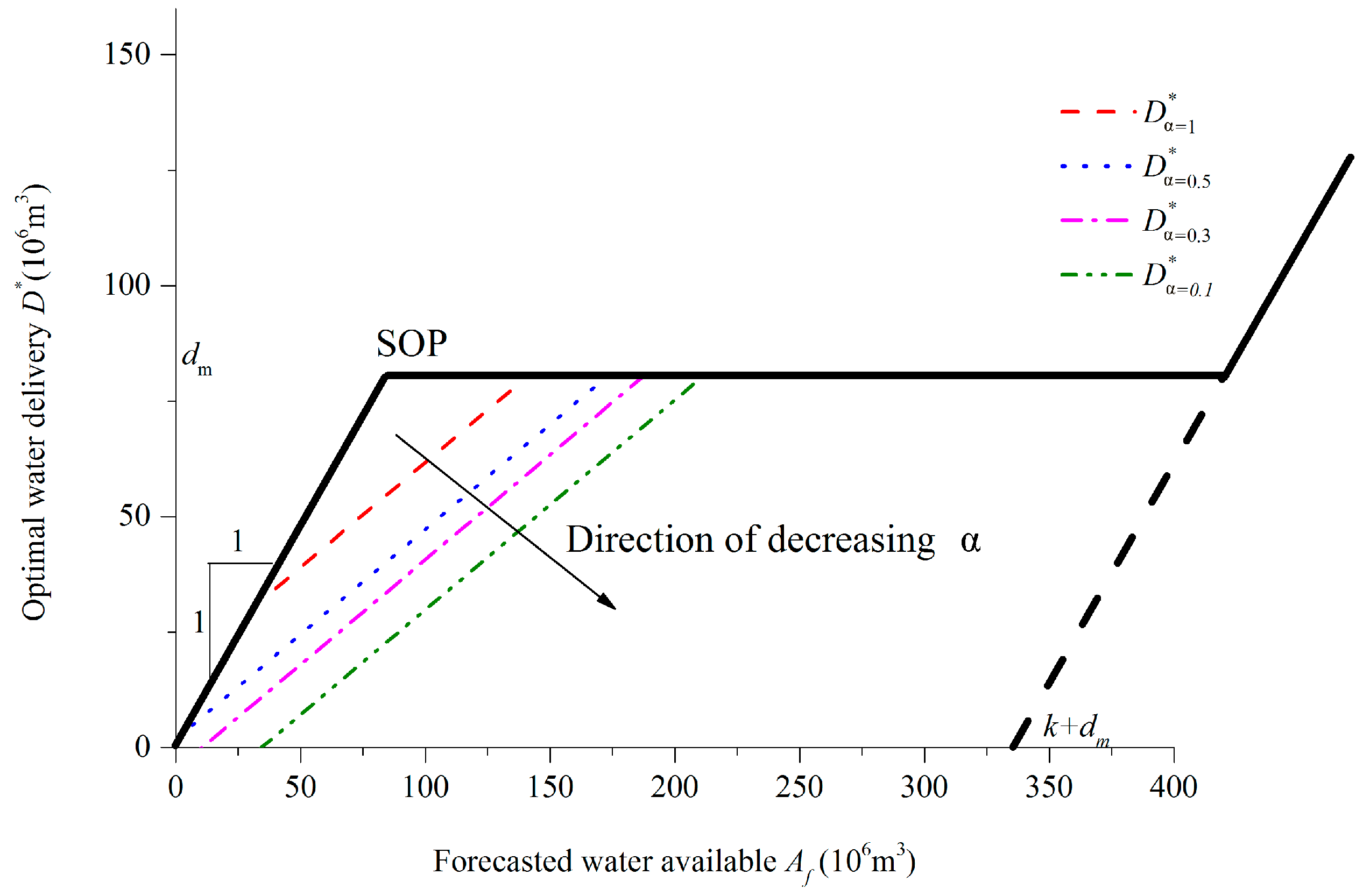
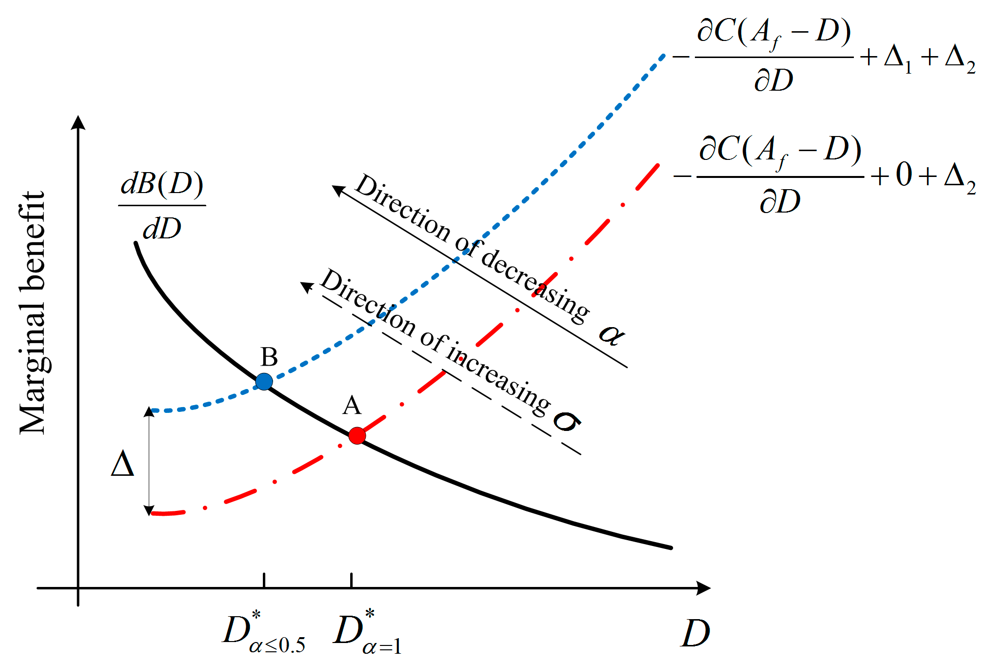
Optimal hedging policies on D can be obtained using Equation (21) under different conditions. For a brief demonstration, in this section, we simulate the hedging policy of reservoir operations at the beginning of March, facing a water demand ( d m ) of 80 × 1 0 6   m 3 . To address the influence of α on the results, 
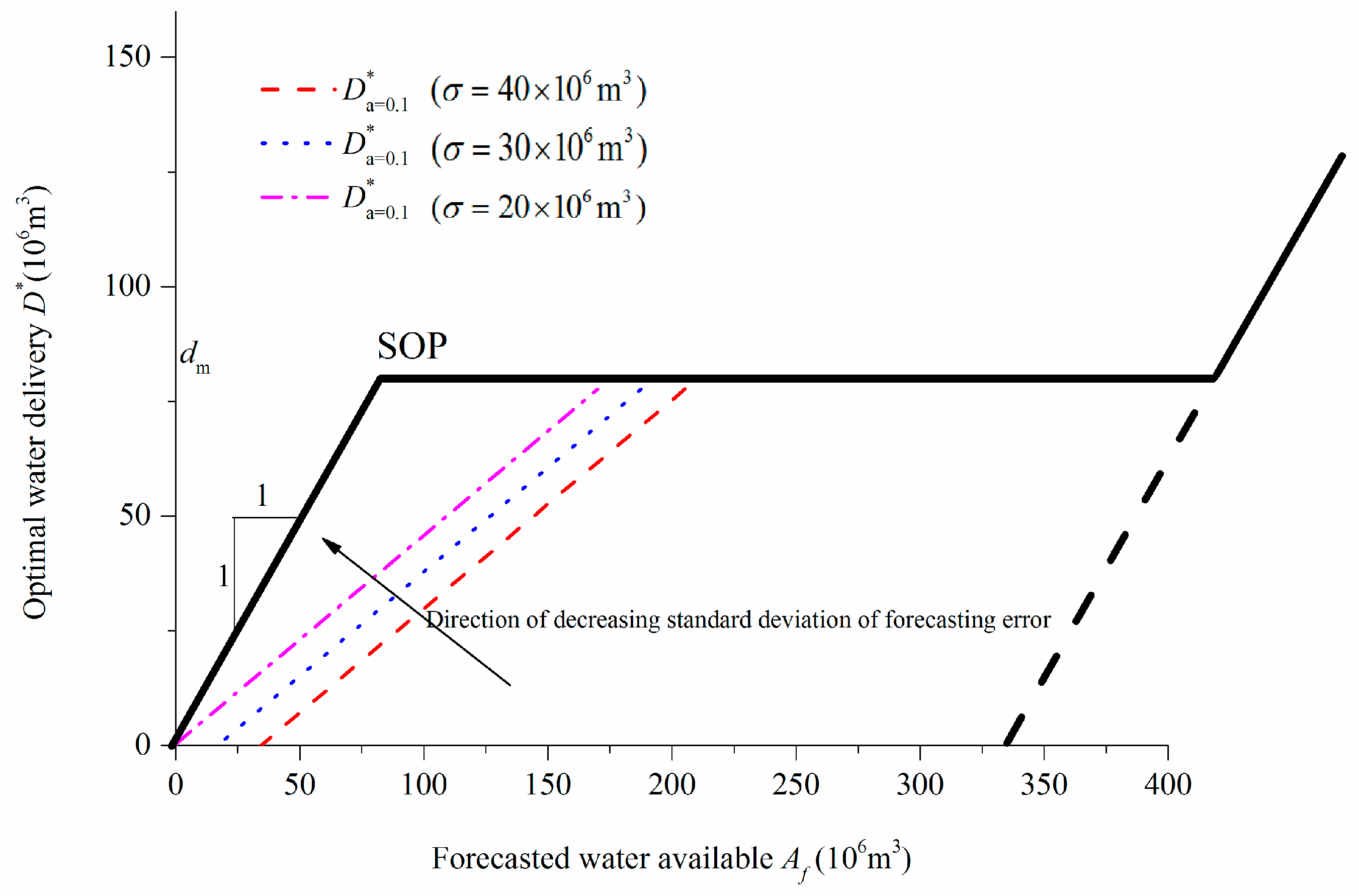
Figure 3 plots the optimal hedging rules under different values of α but the same value of σ ( σ = 40 × 1 0 6   m 3 ).
The hedging rule curves present linear trends with the increase in forecasted available water. Consistent with the analysis made in Section 2.2.3, limited water would be delivered as α decreases. The starting water availability (SWA) [25], which is the threshold of A f for triggering hedging, increases as α decreases when α is less than or equal to 0.5. The ending water availability (EWA), which is the threshold of A f for terminating hedging, increases as α decreases.
The variation ranges of SWA to EWA imply that the water delivery under the CVaR criterion is more conservative than that under the EV criterion. For instance, under the condition of α = 0.5 , hedging would be triggered when A f varies from 0 to 170 × 10 6 m3, whereas the triggered range of A f for α = 1 varies from 32 × 10 6 m3 to 142 × 10 6 m3, indicating that hedging would be undertaken in a wide range of A f when α is low. The “zero-release” range of A f would be great under a low α value, which means water is strictly reserved for anti-adverse hydrological conditions in the future rather than delivered in the current.
The decrease in α indicates that decision makers become risk-averse toward water shortage in the future, i.e., they would sacrifice current benefit to reduce the loss in the future benefit induced by potential drought. Reduced water delivery is a surrogate of insurance for the worst outcomes, and the most conservative decision upon the current water delivery would be made if α approaches zero.
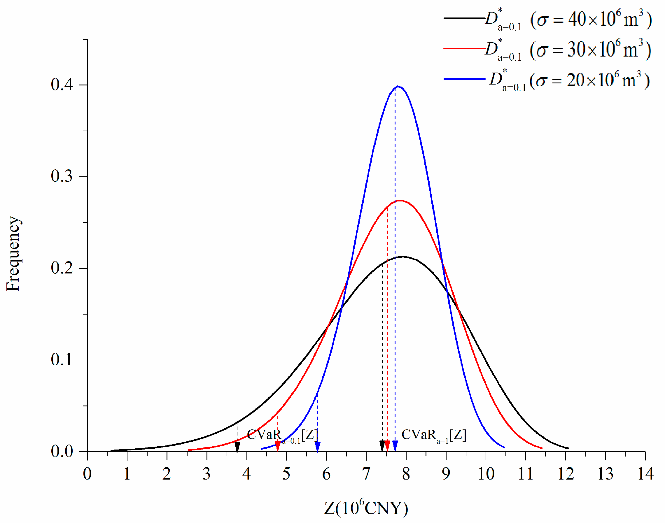
Figure 4 plots the optimal hedging curves under different values of σ but with the same value of α = 0.1 . The optimal water delivery can be increased as σ decreases, which means that abundant water can be delivered to ensure the current benefit if the influence of forecast uncertainty is reduced by improving the precision of inflow forecasts. The decrease in σ results in a sharp forecasting error distribution, in which the probabilities of adverse situations (e.g., inflow is greatly overestimated) are low. Thus, substantial water can be delivered rather than reserved.

3.2. Statistical Measures of Total Benefit

To investigate the statistical measures of total benefit under different water delivery plans, Table 2 lists the corresponding results for the case of A f = 130 × 1 0 6   m 3 and σ = 40 × 1 0 6   m 3 .
The results show that the optimal water delivery solution under the EV criterion ( D α = 1 ) can only guarantee that C V a R α = 1 [ Z ] ( E [ Z ] ) is maximized, but it does not ensure that the statistical results of total benefit under less-profitable situations ( C V a R α < 1 [ Z ] ) are maximized. Similarly, optimal water delivery under the CVaR criterion ( D α < 1 ) guarantees that C V a R α < 1 [ Z ] is maximized at the expense of degradation in the EV of total benefit. For instance, D α = 1 would result in the highest C V a R α = 1 [ Z ] of 7 . 6 × 10 6 CNY, but the lowest value of C V a R α = 0.1 [ Z ] ( 3.57 × 10 6 CNY), whereas D α = 0.1 produces the highest C V a R α = 0.1 [ Z ] of 3.76 × 10 6 CNY but the lowest value of E [ Z ] ( 7 . 4 × 10 6 CNY). Therefore, if decision makers select D α = 0.1 rather than D α = 1 , C V a R α = 0.1 [ Z ] can be increased by 0.19 × 10 6 CNY (5.3%) at the expense of a reduction in E [ Z ] by 0.2 × 10 6 CNY (2.7%). Tradeoffs exist among the indices.
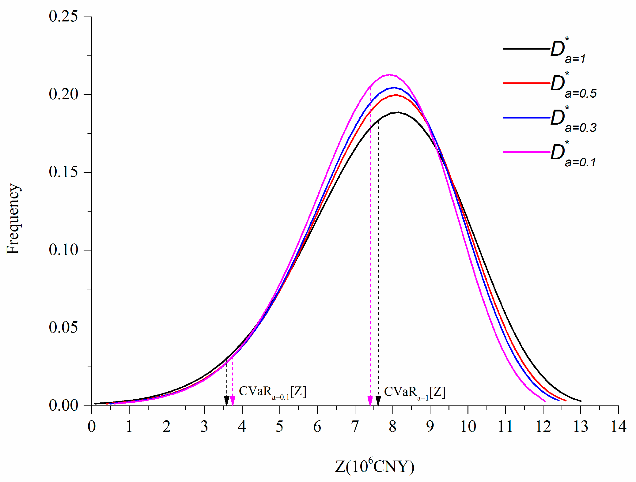
Figure 5 draws the probability density functions of Z under different values of α to determine the reasons for the tradeoffs among different CVaR indices under various hedging policies.
The standard deviation of Z ( σ Z ) decreases as D diminishes. This result can be explained by a theoretical analysis of the variance of Z , as analyzed in Appendix B. The decrease in α could result in water-saving actions, which reduce water delivery D . Therefore, although actual inflow is less than anticipated and water shortage may occur in the future, the influence on Z can be alleviated because reduced water delivery helps increase water storage. Correspondingly, the total benefit in dry hydrological scenarios is improved. If actual inflow is greater than anticipated and water that spills, the reduced water delivery could result in water surplus with minimal marginal benefit. Thus, the total benefit in those wet hydrological scenarios decreases. The probability density function of Z sharpens due to the influence of a reduced σ Z .
Figure 6 plots the probability density function of Z under different values of σ with α = 0.1 . This figure shows how the distribution of total benefit is influenced by improvements in forecasting accuracy.
C V a R α = 0.1 [ Z ] and C V a R α = 1 [ Z ] are improved as forecasting accuracy increases. If σ can be reduced from 40 × 1 0 6   m 3 to 20 × 1 0 6   m 3 , then C V a R α = 0.1 [ Z ] can be increased by nearly 53%, whereas C V a R α = 1 [ Z ] can be increased by 3.4%. The total benefit under a low confidence level of CVaR is more sensitive than the EV of total benefit considering the influence of forecasting accuracy. Therefore, improving the forecasting accuracy is an effective approach to improving total benefit, especially for the results under extremely dry hydrological conditions.

4. Discussion

The results under 49-year (1965–2013) actual streamflow sequences from observation records are simulated to validate the performances of hedging policies under different confidence levels when applied to guide real-time operations. Forecasted streamflow sequences are generated according to the current level of forecasting accuracy and used for guiding operations. Four indices, namely, the reliability η [7], maximum one-month shortage percentage υ [9], total water spillage γ , and actual total benefit during droughts β , are used to assess the performances, which can be characterized as follows:
η = C o u n t { t [ 1 , T ] , t | d m t D t = 0 } / T
υ = max t [ 1 , T ] { | min { D t d m t , 0 } | d m t × 100 % }
γ = t = 1 T { S t k t i f ( S t k t > 0 ) 0 o t h e r w i s e }
β = i = 1 n [ t = T s i T e i B ( D t ) + C ( S T e i + 1 ) ] / n
where C o u n t { } is the number counting function; t is the index of time period; T is the total number of time periods; i is the index of critical drought time spans during which water shortfalls occur; n is the total number of drought events; and T s i and T e i are the starting and ending indices of time period during drought event i , respectively.
Long streamflow sequences are divided into four groups according to the frequency range of annual water volume, namely, the wet (0% to 25%), medium (25% to 50%), dry (50% to 75%), and extremely dry (75% to 100%) patterns to demonstrate the differences in the results under different hydrological patterns. Table 3 presents the results of indices under different hedging decisions denoted by confidence levels.
Table 3 presents the following findings:
(1)
Hedging decisions under the EV criterion ( α = 1 ) result in the highest reliability of water supply for all hydrological patterns. They could also cause the highest one-month water shortage level under dry and extremely dry conditions. By contrast, hedging decisions under the CVaR criterion ( α 1 ) cause frequent but small water shortages, yet the highest one-month water shortages under dry and extremely dry conditions are all less than the results obtained under the hedging decisions using the expectation criterion. However, under wet and medium hydrological conditions, hedging decisions under the CVaR criterion could cause severe one-month water shortage. Hedging decisions under the CVaR criterion would be suited for dry and extremely dry hydrological conditions wherein the occurrence likelihood of drought is high.
(2)
Substantial water would be spilled if the hedging policies under the CVaR criterion are implemented compared with the results of hedging under the expectation criterion. Hedging the loss of water shortage during drought by water conservation would have a side effect in increasing the water spilled considering the influence of forecasting error.
(3)
The effect of hedging under the CVaR criterion can be explored under dry or extremely dry hydrological patterns. Consistent with theoretical analysis, the actual total benefit obtained from hedging decisions under the CVaR criterion is greater than the total benefit obtained from hedging decisions under the expectation criterion, during critical time periods of dry and extremely dry hydrological patterns. In facing wet or medium hydrological patterns, the difference in actual total benefit could be small.
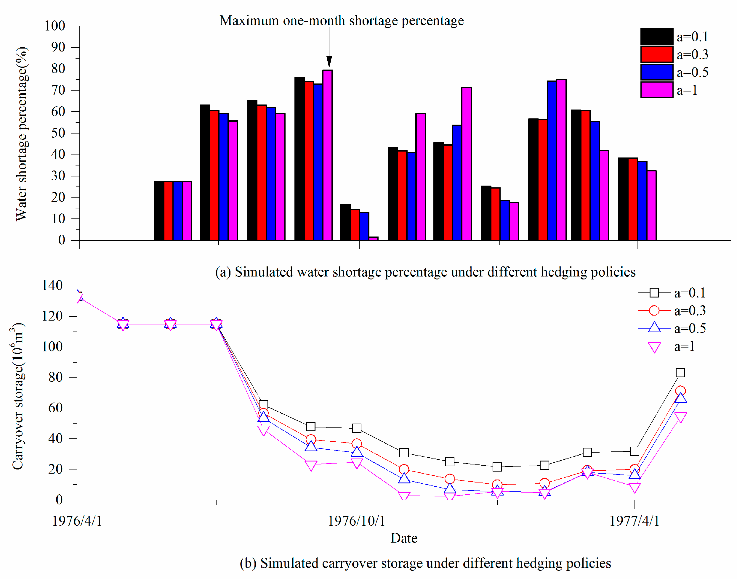
The results of water shortage percentage and carryover storage for the reservoir during a typical dry hydrological time span (with the hydrology frequency of 87%) are compared for the four scenarios of hedging policies, as shown in Figure 7.
During the critical time periods, the total inflows are overestimated by 1%. The highest one-month shortage percentage under the hedging policy using the EV criterion ( α = 1 ) would be 79.4%, whereas that obtained under the hedging policy using the CVaR criterion ( α = 0.3 ) would be 74.2%. Both the highest one-month shortages occurred in September 1976 as actual inflows from June to August 1976 are overestimated by 28%. Under the guidance of forecasted inflow, the policy ( α = 1 ) delivers 5.9% more water than the water delivered by the hedging policy using the CVaR ( α = 0.3 ) criterion. Compared with the result of actual benefit obtained from the hedging policy using the EV criterion ( α = 1 ), the actual benefit can be increased by 0.4% if the policy of the CVaR criterion ( α = 0.3 ) is employed due to a successful water carryover.

5. Conclusions

This paper discusses the optimal hedging policy for a water supply reservoir considering the influence of inflow forecast uncertainty. An optimal hedging model for maximizing the overall benefit of water delivery (current benefit) and water storage (future benefit) is established. Inflow forecast uncertainty is addressed when estimating current water availability. Two different optimization criteria, the EV and CVaR criteria, are introduced to set different measures of total benefit of water delivery and carryover storage. The optimality conditions for the optimal hedging policies under the two criteria are analyzed, and the analytic solutions of hedging rules are derived. Differences in the hedging rules under the two criteria are highlighted with regard to varied inflow forecasting precisions and attitudes of decision makers toward risk hedging (the confidence level). Performances of hedging policies under the two criteria in real-time operations are analyzed by numerical simulations.
The methodology is applied to the Foziling Reservoir in China. The results are as follows:
(1)
Under the influence of forecast uncertainty, the optimal value of water delivery reduces as σ increases or α decreases. Therefore, decision makers will be conservative on current water delivery under a low inflow forecasting precision or a significant risk-averse attitude.
(2)
The maximization of C V a R α [ Z ] is at the expense of potential degradation in E [ Z ] . Hedging the risk of water shortage in the future encourages water saving in the current, but it could also increase the chance of future water spill.
(3)
In real-time operations, compared with the hedging policies using the EV criterion, hedging decisions using the CVaR criterion would be more suited for dry and extremely dry hydrological conditions wherein the occurrence likelihood of drought is high.
Although the optimal hedging rules under CVaR and EV criteria are systematically compared and analyzed via analytic derivations, more complex and practical modeling techniques are encouraged to bridge the gap between mathematical simplifications and real-world implementations. For example, extending the study to guide the operations of multiple-reservoir systems presents challenges in dealing with complex constraints that bind the physical and economic conditions of hedging. Future efforts can improve the current study.

Acknowledgments

We would like to thank three anonymous reviewers for their in-depth reviews and constructive suggestions. The remarks and summary of reviewer comments provided by the Editor and Associate Editor are also greatly appreciated. The help of language editing offered by Martin J. Booth is appreciated. These have facilitated major improvements in this paper. This study is supported by the National Key Technologies R&D Program of China (Grant No. 2016YFC0400909), the National Natural Science Foundation of China (Grant No. 51609062 and Grant No. 51579068), the Fundamental Research Funds for the Central Universities (Grant No. 2015B28414), China Postdoctoral Science Foundation Funded Project (Grant No. 2017M611864), and the Special Fund for Public Welfare Industry of the Ministry of Water Resources of China (Grant No. 201501007).

Author Contributions

Bin Xu and Ping-An Zhong conceived and designed the experiments; Jianqun Wang and Qiyou Huang performed the experiments; Zhongbo Yu and Jianyun Zhang contributed to the discussion; Bin Xu wrote the paper.

Conflicts of Interest

The authors declare no conflict of interest.

Appendix A. First-Order Optimality Condition

According to the definition of CVaR, Equation (15) provides the first-order optimality condition of D using an integration of the forecasting error ε . If we replace the Taylor’s series of C ( A f D + ε ) expressed in Equation (16) back to the integration term in Equation (15), it can be rewritten as:
V a R α [ ε ] C ( A f D + ε ) p ( ε ) d ε V a R α [ ε ] [ C ( A f D ) + C ( A f D ) ε + C ( A f D ) 2 ε 2 ] p ( ε ) d ε
The integration can be decomposed into the summation of the following terms:
V a R α [ ε ] C ( A f D ) p ( ε ) d ε = C ( A f D ) V a R α [ ε ] p ( ε ) d ε = C ( A f D ) α V a R α [ ε ] C ( A f D ) ε p ( ε ) d ε = C ( A f D ) V a R α [ ε ] ε p ( ε ) d ε = C ( A f D ) α C V a R α [ ε ] V a R α [ ε ] C ( A f D ) 2 ε 2 p ( ε ) d ε = C ( A f D ) 2 V a R α [ ε ] ε 2 p ( ε ) d ε = C ( A f D ) 2 α C V a R α [ ε 2 ]
Therefore, Equation (16) can be expanded as:
F ( D ) D d B ( D ) d D + 1 α { C ( A f D ) α C V a R α [ ε ] + C ( A f D ) α C V a R α [ ε ] + C ( A f D ) 2 α C V a R α [ ε 2 ] } D
For F ( D ) D = 0 , Equation (17) can be obtained by expanding the derivative terms and reorganizing Equation (A3).

Appendix B. Influence of D on σ Z 2

The variance of total benefit Z can be expressed as:
G [ Z ] = G [ B ( D ) + C ( S ) ] = G [ C ( S ) ]
where G [ ] is the variance function. B ( D ) is a deterministic term, and its variance is zero. G [ Z ] is only determined by the uncertainty in storage S .
With Equation (12), S = A f D + ε , G [ Z ] can be characterized as G [ C ( A f D + ε ) ] . Similarly, using Equation (17) to expand C ( A f D + ε ) in terms of ε , we can express G [ Z ] as
G [ Z ] = G [ C ( A f D ) + C ( A f D ) ε + C ( A f D ) 2 ε 2 ]
For G [ C ( A f D ) ] = 0 , G [ C ( A f D ) ε ] = [ C ( A f D ) ] 2 G [ ε ] , and G [ C ( A f D ) 2 ε 2 ] = [ C ( A f D ) ] 2 4 G [ ε 2 ] , G [ Z ] can be decomposed into the summation of the following terms:
G [ Z ] = [ C ( A f D ) ] 2 G [ ε ] + [ C ( A f D ) ] 2 4 G [ ε 2 ]
Therefore, the partial derivative of G [ Z ] on D is given by
G [ Z ] D = 2 C ( A f D ) C ( A f D ) G [ ε ] C ( A f D ) C ( A f D ) 2 G [ ε 2 ]
The carryover storage value function C [ ] is an increasing function with decreased marginal benefit. Accordingly, C ( A f D ) > 0 and C ( A f D ) < 0 . C ( A f D ) , G [ ε ] , and G [ ε 2 ] are all positive, and both product terms in Equation (33) are positive such that G [ Z ] D > 0 . Hence, the variance of total benefit increases with water delivery D .

References

  1. Yeh, W.W. Reservoir management and operations models: A state-of-the-art review. Water Resour. Res. 1985, 21, 1797–1818. [Google Scholar] [CrossRef]
  2. Labadie, J.W. Optimal operation of multireservoir systems: State-of-the-art review. J. Water Resour. Plan. Manag. 2004, 130, 93–111. [Google Scholar] [CrossRef]
  3. Draper, A.J.; Lund, J.R. Optimal hedging and carryover storage value. J. Water Resour. Plan. Manag. 2004, 130, 83–87. [Google Scholar] [CrossRef]
  4. Neelakantan, T.R.; Sasireka, K. Review of Hedging Rules Applied to Reservoir Operation. Int. J. Eng. Technol. 2015, 7, 1571–1580. [Google Scholar]
  5. Wang, H.; Liu, J. Reservoir Operation Incorporating Hedging Rules and Operational Inflow Forecasts. Water Resour. Manag. 2013, 27, 1427–1438. [Google Scholar] [CrossRef]
  6. Hu, T.; Zhang, X.; Zeng, X.; Wang, J. A Two-Step Approach for Analytical Optimal Hedging with Two Triggers. Water 2016, 8, 52. [Google Scholar] [CrossRef]
  7. Hashimoto, T.; Stedinger, J.R.; Loucks, D.P. Reliability, Resiliency, and Vulnerability Criteria for Water Resource System Performance Evaluation. Water Resour. Res. 1982, 18, 14–20. [Google Scholar] [CrossRef]
  8. Klemes, V. Value of Information in Reservoir optimization. Water Resour. Res. 1977, 13, 837–850. [Google Scholar] [CrossRef]
  9. Shiau, J.T. Analytical Optimal Hedging with Explicit Incorporation of Reservoir Release and Carryover Storage Targets. Water Resour. Res. 2011, 47, W01515. [Google Scholar] [CrossRef]
  10. Zeng, X.; Hu, T.; Xiong, L.; Cao, Z.; Xu, C. Derivation of operation rules for reservoirs in parallel with joint water demand. Water Resour. Res. 2015, 51, 9539–9563. [Google Scholar] [CrossRef]
  11. Yu, Z.; Barron, E.J.; Yarnal, B.; Lakhtakia, M.N.; White, R.A.; Pollard, D.; Miller, D.A. Evaluation of basin-scale hydrologic response to a multi-storm simulation. J. Hydrol. 2002, 257, 212–225. [Google Scholar] [CrossRef]
  12. Xu, B.; Boyce, S.E.; Zhang, Y.; Liu, Q.; Guo, L.; Zhong, P.A. Stochastic Programming with a Joint Chance Constraint Model for Reservoir Refill Operation Considering Flood Risk. J. Water Resour. Plan. Manag. 2016, 143, 4016061–4016067. [Google Scholar] [CrossRef]
  13. Xu, B.; Zhong, P.; Zambon, R.C.; Zhao, Y.; Yeh, W.W.G. Scenario tree reduction in stochastic programming with recourse for hydropower operations. Water Resour. Res. 2015, 51, 6359–6380. [Google Scholar] [CrossRef]
  14. You, J.; Cai, X. Hedging rule for reservoir operations: 1. A theoretical analysis. Water Resour. Res. 2008, 44, W01415. [Google Scholar] [CrossRef]
  15. Zhao, T.; Zhao, J.; Lund, J.R.; Yang, D. Optimal Hedging Rules for Reservoir Flood Operation from Forecast Uncertainties. J. Water Resour. Plan. Manag. 2014, 140, 04014041. [Google Scholar] [CrossRef]
  16. Xu, J.; Ma, N.; Lv, C. Dynamic equilibrium strategy for drought emergency temporary water transfer and allocation management. J. Hydrol. 2016, 539, 700–722. [Google Scholar] [CrossRef]
  17. Pedro-Monzonís, M.; Solera, A.; Ferrer, J.; Estrela, T.; Paredes-Arquiola, J. A review of water scarcity and drought indexes in water resources planning and management. J. Hydrol. 2015, 527, 482–493. [Google Scholar] [CrossRef]
  18. Rockafellar, R.T.; Uryasev, S. Conditional value-at-risk for general loss distributions. J. Bank. Financ. 2002, 26, 1443–1471. [Google Scholar] [CrossRef]
  19. Andersson, F.; Mausser, H.; Rosen, D.; Uryasev, S. Credit risk optimization with Conditional Value-at-Risk criterion. Math. Program. 2001, 273–291. [Google Scholar] [CrossRef]
  20. Yamout, G.M.; Hatfield, K.; Romeijn, H.E. Comparison of new conditional value-at-risk-based management models for optimal allocation of uncertain water supplies. Water Resour. Res. 2007, 43, W07430. [Google Scholar] [CrossRef]
  21. Piantadosi, J.; Metcalfe, A.V.; Howlett, P.G. Stochastic dynamic programming (SDP) with a conditional value-at-risk (CVaR) criterion for management of storm-water. J. Hydrol. 2008, 348, 320–329. [Google Scholar] [CrossRef]
  22. Hu, Z.; Wei, C.; Yao, L.; Li, L.; Li, C. A multi-objective optimization model with conditional value-at-risk constraints for water allocation equality. J. Hydrol. 2016, 542, 330–342. [Google Scholar] [CrossRef]
  23. Kimball, M.S. Precautionary saving in the small and in the large. Econometrica 1990, 58, 53–73. [Google Scholar] [CrossRef]
  24. Draper, A.J. Implicit Stochastic Optimization with Limited Foresight for Reservoir Systems. Ph.D. Thesis, University of California, Davis, CA, USA, 2001. [Google Scholar]
  25. Bayazit, M.; Unal, N.E. Effects of Hedging on Reservoir Performance. Water Resour. Res. 1990, 26, 713–719. [Google Scholar] [CrossRef]
Figure 1. E [ Z ] , V a R α [ Z ] , and C V a R α [ Z ] of a benefit distribution function.
Water 09 00568 g001
Figure 2. Equilibriums under expectation and CVaR criteria for optimal water delivery.
Water 09 00568 g002
Figure 3. Optimal hedging policies under different values of α ( σ = 40 × 1 0 6   m 3 ).
Water 09 00568 g003
Figure 4. Optimal hedging policies under different values of σ ( α = 0.1 ).
Water 09 00568 g004
Figure 5. Probability density functions of Z under different values of α ( σ = 40 × 1 0 6   m 3 ).
Water 09 00568 g005
Figure 6. Probability density functions of Z under different values of σ ( α = 0.1 ).
Water 09 00568 g006
Figure 7. Simulated water shortage percentage and carryover storage trajectories of hedging policies under a typical dry-hydrology time span. (a) Plots the simulated results of water shortage percentage under different hedging policies during the dry-hydrology time span while (b) draws the corresponding simulated trajectories of carryover storages of the hedging policies.
Water 09 00568 g007
Table 1. Parameters of the case study.
ParametersParameter Values
Storage capacity k (106 m3)260
Standard deviation scenarios of the forecasting error σ (106 m3)40/30/20
Confidence level α 1/0.5/0.3/0.1
Parameters of the benefit function a d b d c d
06.87 × 10⁻²−1.05 × 10⁻⁴
Parameters of the carryover storage value function a s b s c s
06.25 × 10⁻²−8.72 × 10⁻⁵
Table 2. Water delivery plans and statistics of the results.
Water Delivery Plans C V a R α [ Z ] (106 CNY)
D α α = 1 (EV) α = 0.5 α = 0.3 α = 0.1
D α = 1 7.605.915.063.57
D α = 0.5 7.565.955.133.70
D α = 0.3 7.515.945.143.74
D α = 0.1 7.405.895.123.76
Table 3. Simulated statistics of indices under different hedging strategies and hydrological patterns.
α η υ
WetMediumDryExtremely DryWetMediumDryExtremely Dry
0.1086.8%73.1%72.9%70.1%50.6%74.0%67.0%73.0%
0.3087.5%75.0%75.0%70.1%49.5%72.4%68.7%74.2%
0.5087.5%75.0%76.4%70.1%50.0%71.8%74.3%78.3%
1.0088.2%75.6%77.8%70.8%48.0%70.8%75.0%89.8%
α γ (106 m3) β (106 CNY)
WetMediumDryExtremely DryWetMediumDryExtremely Dry
0.1069.5742.6739.4734.394.1214.6116.8219.12
0.3069.2042.4239.2234.174.1214.6216.8719.08
0.5068.9642.3039.0734.014.1314.6216.9019.04
1.0068.4342.0138.6133.564.1414.6116.8319.01

