Article

Multi–Model Ensemble Approaches to Assessment of Effects of Local Climate Change on Water Resources of the Hotan River Basin in Xinjiang, China

1
State Key Laboratory of Desert and Oasis Ecology, Xinjiang Institute of Ecology and Geography, Chinese Academy of Sciences, 830011 Urumqi, China
2
Department of Geography, Ghent University, 9000 Gent, Belgium
3
University of Chinese Academy of Science, 100049 Beijing, China
4
Sino-Belgian Joint Laboratory of Geo-information, 830011 Urumqi, China
5
Research Fund Flanders (FWO), 1000 Brussels, Belgium
6
Sino-Belgian Joint Laboratory of Geo-information, 9000 Gent, Belgium
*
Author to whom correspondence should be addressed.
Water 2017, 9(8), 584; https://doi.org/10.3390/w9080584
Submission received: 19 May 2017 / Revised: 28 July 2017 / Accepted: 31 July 2017 / Published: 5 August 2017
(This article belongs to the Special Issue Adaptation Strategies to Climate Change Impacts on Water Resources)

Abstract

:
The effects of global climate change threaten the availability of water resources worldwide and modify their tempo-spatial pattern. Properly quantifying the possible effects of climate change on water resources under different hydrological models is a great challenge in ungauged alpine regions. By using remote sensing data to support established models, this study aimed to reveal the effects of climate change using two models of hydrological processes including total water resources, peak flows, evapotranspiration, snowmelt and snow accumulation in the ungauged Hotan River Basin under future representative concentration pathway (RCP) scenarios. The results revealed that stream flow was much more sensitive to temperature variation than precipitation change and increased by 0.9–10.0% according to MIKE SHE or 6.5–10.5% according to SWAT. Increased evapotranspiration was similar for both models with a range of 7.6–31.3%. The snow-covered area shrank from 32.5% to 11.9% between the elevations of 4200–6400 m, respectively, and snow accumulation increased when the elevation exceeded 6400 m above sea level (asl). The results also suggested that the fully distributed and semi-distributed structures of these two models strongly influenced the responses to climate change. The study proposes a practical approach to assess the climate change effect in ungauged regions.

1. Introduction

An ever increasing amount of evidence suggests that the continual increase in greenhouse gas emissions is affecting the global climate and altering the local precipitation and temperatures [1,2]. According to the fifth assessment report (AR5) of the Intergovernmental Panel on Climate Change (IPCC), the global temperature increased by 0.85 °C during 1880–2012, and will further increase by 0.3–4.8 °C until 2100 [3]. This global warming is expected to produce significant effects on water resources and freshwater ecosystems [3,4]. The effects and intensity of climate change will vary from region to region [5].
Arid and semi-arid regions in northwestern China are very vulnerable to the effects of climate change because of their fragile ecosystems and scare water resources [6,7]. In recent years, arid and semi-arid regions have received more attention related to future climate change and the effects of that change on water resources [8,9,10,11]. The largest inland river in China, the Tarim River, flows through the arid and semi-arid region of northwestern China. This region characteristically experiences an extremely dry desert climate with low amounts of infrequent rainfall and strong potential evaporation [6]. Many previous studies have indicated that this region is especially sensitive to climate change because the main water sources in this region come from high elevation glaciers and snowmelt [5,12,13,14]. Therefore, for the purposes of managing water resources and flood security, it is essential to assess the possible changes of water resource availability and analyze the responses of hydrological processes under future climate change scenarios.
To analyze the effects of climate change on water resources, a number of researchers have directly input future climate data into hydrological models to acquire the related hydrological results [15,16]. However, the model outputs of General Circulation Models (GCMs), with pixel sizes of ca. 150–300 km, are too coarse to be used in hydrological models for the analysis of local effects [17,18]. Data mismatch problems also exist between GCMs and hydrological models with respect to spatial and temporal scales [19,20]. Therefore, to forecast the effects of possible climate change in arid and semi-arid regions in northwestern China, two ambitious problems should be solved: downscaling climate data and setting up a hydrological model in the ungauged basins.
Many downscaling methods exist such as the Statistical Downscaling Model (SDSM) [21], Automated Statistical Downscaling (ASD) [17,22], Change Factor (Delta) method [23], and Wet Day Perturbation (WDP) method [19,24]. These can be used to downscale the projected GCM data into stationary data for hydrological input. The most common downscaling approach might be the Delta method. This method is based on assuming that the relative changes obtained from the GCMs are more representative than absolute changes [25]. The Delta method has the computing advantage of being able to cluster the entire range of GCM models into a mean level using an ensemble approach [25,26,27]. However, the Delta method ignores the frequency change of precipitation, which is the key factor for flood events. By considering both changes in the frequency and intensity of precipitation in different quantiles, precipitation projections including extreme events could be properly addressed by an advanced quantile perturbation method (wetQPM) [25,28]. Therefore, the suitability of wetQPM in arid regions should be examined in addition to the Delta method.
Hydrological modelling in the arid and semi-arid region of China is relatively difficult with only sparse hydro-metrological data currently available [29]. The spatial heterogeneity of the watersheds as well as the variable hydrological characteristics and morphology of the mountainous areas create great challenges in accurately forecasting hydro-meteorological observations such as precipitation and temperature [30]. In recent years, the availability of remote sensing products has provided an opportunity for hydrological modelling to replace land-based stationary observations [31]. Several satellite-based products can be used to measure precipitation, such as Global Satellite Mapping of Precipitation (GSMaP) [32], Climate Hazards Group Infrared Precipitation with Station data (CHIRPS) [33], the Tropical Rainfall Measuring Mission (TRMM) [34] and the Climate Prediction Center’s morphing technique known as CMORPH [35]. Among these, the TRMM rainfall products possess apparent advantages based on their long service duration and stable quality performance from January 1998 to April 2015 [36]. TRMM data are widely used in hydrological simulations [37,38,39,40]. The Global Precipitation Measurement (GPM) mission replaced the TRMM satellite on February 2014 [41]. To overcome the difficulties of modelling setups in an ungauged watershed in the present study, we applied corrected TRMM rainfall data in the hydrological model to close the data gap for distributed hydrological modelling in the Hotan River Basin. This basin is one of the most important headwater regions of the Tarim River Basin [42,43]. Two widely used hydrological models, MIKE SHE and SWAT, were used to analyze the sensitivity of the effects of climate change to explore the uncertainties of model reactions.
The objective of this study is to reveal the tempo-spatial features of effects of climate change on water resources and extremes in ungauged regions. The Delta and wetQPM downscaling methods were adopted to provide realistic climate change data. Through the application of remote sensing data in this study to set up the hydrological models as the direct input and references of calibration or validation, both the SWAT and MIKE SHE models were used in the assessment of climate change effects. In this way, the spatiotemporal redistributions of runoff, snowmelt and evapotranspiration from the two models are used to explain the effects of the structure of the modules on the response of water resources and to reinforce our understanding of water cycle processes.

2. Study Area and Data
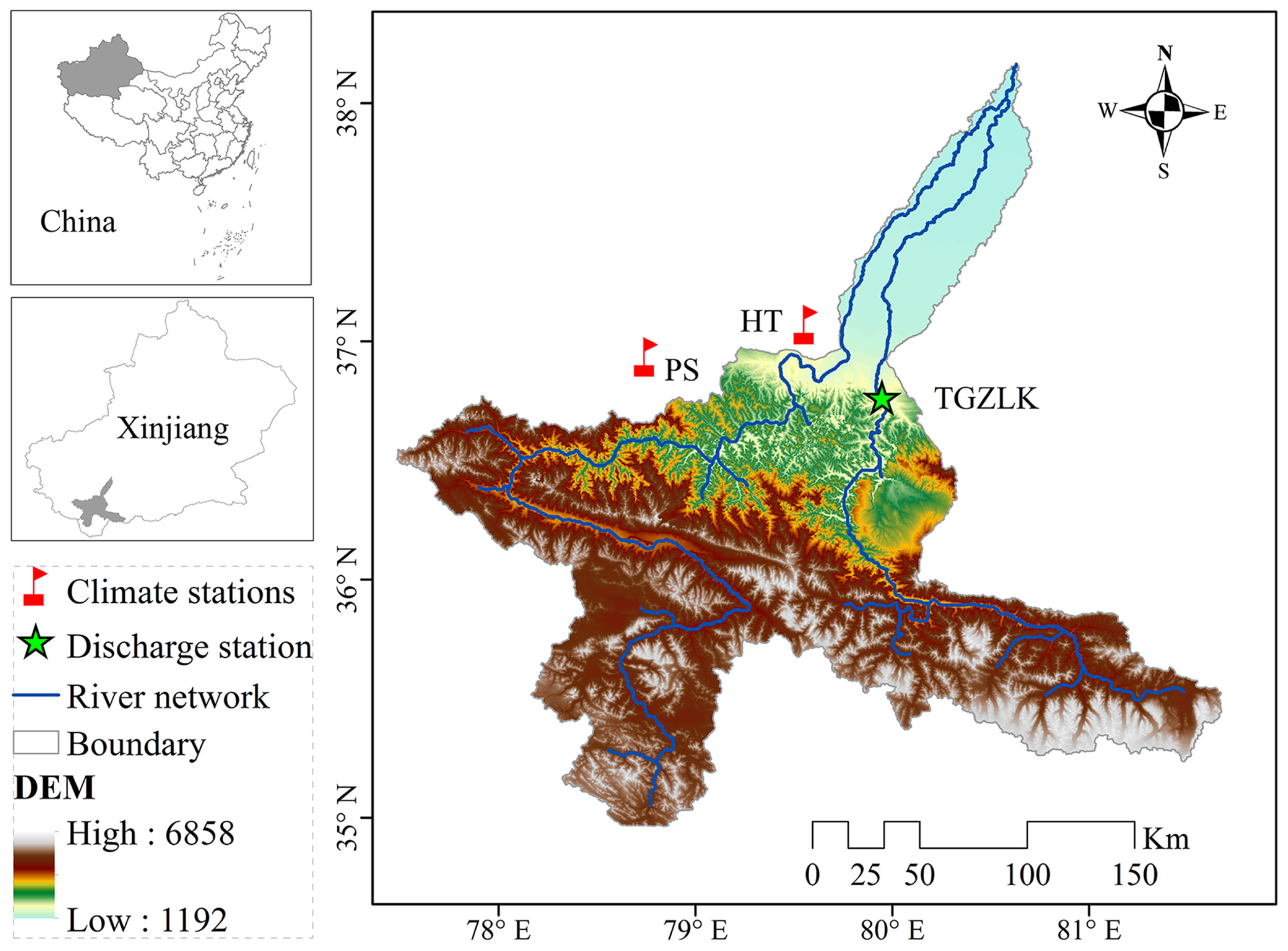
2.1. Study Area

The Hotan River Basin, located in Northwest China, lies between longitude 77°27′–81°43′ E and latitude 34°52′–40°29′ N and covers an area of 4.89 × 10⁴ km2 (Figure 1) in the region of the Tarim River Basin [12]. The complex landforms of the catchment of the Hotan River Basin mainly include woodlands, grasslands, glaciers and desert. The adjacent surrounding areas include alpine mountains with elevations varying from 1192 m to 6858 m·asl (mean 4172 m·asl). The semi-arid climate of the study area is influenced by continental climate variation with a mean annual temperature of 12.2 °C and precipitation of 5.4–89.6 mm [44]. The Hotan River flows for 1127 km [45], with a mean annual water discharge of 4.478 × 10⁹ m3. The Hotan River mainly originates from seasonal snowfall and other precipitation at high elevations in the mountains along with the melting of non-perennial snow and glacial meltwater [46,47]. The water resources in the River are mainly used for agricultural irrigation and to support the aquatic environment of the Hotan sanctuary, which is located south of the Taklimakan Desert, the largest desert in China [48]. As a result of the harsh climatic conditions and water scarcity in the region, the river basin is very vulnerable to climate change [44].

2.2. Data

The daily meteorological data employed in this work were derived from the China Meteorological Data Sharing Service System [49], and included daily parameters of precipitation (Pr), average temperature (Tas), maximum temperature (Tmax) and minimum temperature (Tmin) for Hotan (HT) and Pishan (PS) meteorological stations (Figure 1). The Tarim Water Resources Management Bureau and the Xinjiang Institute of Ecology and Geography of the Chinese Academy of Sciences provided the hydrological and geographical datasets used here. In addition, we also used spatially distributed TRMM 3B42 daily rainfall data for hydrological modelling.
Global climate models, also known as general circulation models (GCMs), provide the most advanced datasets available for modelling future climate [25]. The outputs of GCMs that were based on the fifth phase of the Coupled Model Intercomparison Project were used to extract future climate projections for the study area with the climate downscaling methods. A total of 37 historical models, as well as 21, 29, and 30 models for RCP2.6, RCP4.5, and RCP8.5, respectively, were adopted in this study. The daily climate data also included datasets related to both historical and future periods [50]. For historical simulation, observations for the control period (1965–2004) were extracted. For future projections, the projected simulations under three future scenarios, RCP2.6, RCP4.5 and RCP8.5, were used for the period 2021–2060. The three RCPs represent “low” (RCP2.6), “medium” (RCP4.5) and “high” (RCP8.5) scenarios featured by radiative forcing of 2.6, 4.5 and 8.5 W/m2 by 2100, respectively [51,52].

3. Methodology

3.1. Hydrological Modelling

Two spatially distributed hydrological models, SWAT [53] and MIKE SHE [54], were employed for hydrological modelling in the Hotan River Basin. By using both of these models, the influence of the model structure on the results related to climate change can be assessed. Both models have a large number of effective applications for hydrological simulation [55,56,57,58], as well as for climate change effect analysis in arid and semi-arid regions in northwestern China [23,59]. Considering the difference in the model structure, both models were used to simulate the comprehensive hydrological processes in the study area with their unique characteristics.
The SWAT model is a conceptual, physically based, semi-distributed model developed by the United States Department of Agriculture, Agricultural Research Service (USDA-ARS) [52]. SWAT operates on a daily time step and is used to predict the effects of watershed management practices and climate change on a gauged or ungauged watershed [60]. The SWAT model requires specific information related to topography, meteorological variables (such as precipitation and maximum/minimum temperature), soil textural and physicochemical properties and land use data [61]. This model simulates at a sub-basin level: an entire watershed/catchment is divided into sub-basins, and sub-basins are further divided into hydrologic response units (HRUs), according to a unique combination of homogeneous land use, soil properties and slope. More detailed descriptions of the model are given in the SWAT theoretical documentation [62].
MIKE SHE is a deterministic, physically based, fully distributed model designed to simulate different processes of the land phase in the hydrologic cycle [63]. The MIKE SHE model works using five model components including overland, channel, unsaturated, and saturated flow as well as evapotranspiration [64]. According to the spatial variation in the catchment area, MIKE SHE divides a basin horizontally into an orthogonal grid network and uses vertical columns; every horizontal grid square represents a unique variation in the vertical direction. This is achieved by dividing the catchment into members of square grids [65,66].
In order to evaluate the performance of the calibrated and validated results provided by the two models, statistical performance indices, such as goodness of fit (R2), Nash-Sutcliffe efficiency coefficient (NS) [67] and relative error (RE) were applied in this research. The equations of these indices are presented using Equations (1)–(3).
R 2 = i = 1 n ( Q s i Q ¯ s ) ( Q a i Q ¯ a ) i = 1 n ( Q s i Q ¯ s ) 2 i = 1 n ( Q a i Q ¯ a ) 2 ;   0 R 2 1 ,
N S = 1 i = 1 n ( Q a i Q s i ) 2 i = 1 n ( Q a i Q ¯ a ) 2 ;     N S     1 ,
R E = i = 1 n ( Q a i Q s i ) i = 1 n Q a i   R E + ,
where, Q ¯ a and Q ¯ s are the mean value of the observed and simulated values, respectively, Q ai and Q si are the observed and simulated values, respectively, at time step i, and n is the number of observations. Normally, when R2 > 0.6, NS > 0.5 and RE < 25%, the modelling results of the discharge are considered to be satisfactory, and the modelling results can be evaluated as excellent if R2 > 0.8, NS > 0.75 and RE < 10% [59,68].

3.2. Inter-Comparison and Evaluation of the Performance of GCMs

Inter-comparison and evaluation of the performance of GCMs were carried out with respect to their ability to reproduce monthly rainfall totals and temperature; in addition, we found that certain filters of GCMs runs were not suitable for the current study region [25,69]. This process was based on certain criteria, which involved comparing both the observed data and the historical GCM datasets [70]. The Taylor diagram method was used as criteria for the evaluation of GCMs and meteorological gauging data results [69]. Taylor diagrams [71] provide a method of graphically summarizing data, showing how closely a pattern (or a set of patterns) matches observations. The similarities between pattern and observation are quantified in terms of their correlation coefficients (Rs), the value of the Root Mean Square Error (E) and the amplitude of standard deviations (Std). Multiple aspects of complex models can be evaluated using a Taylor diagram [72,73]. In recent years, Taylor diagrams have been widely used especially for the evaluation of the performance of GCM models [74,75,76,77,78]. Equations used for calculating the Rs, E, Std, and the standard deviations of the model ( σ f ) and the observation ( σ r ) are presented in Equations (4)–(8).
R s = 1 N n = 1 N ( f n f ¯ ) ( r n r ¯ ) σ f σ r ,
E = [ 1 N n = 1 N ( f n r n ) 2 ] 1 / 2 ,
σ f 2 =   1 N n = 1 N ( f n f ¯ ) 2   ,
σ r 2 = 1 N n = 1 N ( r n r ¯ ) 2   ,
S t d = σ f σ r ,
where, f n and r n represent the model field and observation (reference) field, respectively, N is the number of time steps, f ¯ and r ¯ are the mean values, and σ f and σ r are the Stds of f n and r n , respectively.

3.3. Downscaling Methods

3.3.1. Delta Method for Downscaling Precipitation and Temperature

The Delta method is an ordinary downscaling method [79,80]. This method is based on the assumption that the change factors obtained from the GCMs are more representative than the absolute values, and this method can help researchers to avoid the noise contained in massive datasets [25]. The main processes of the Delta method are modifying the daily time series of climatic variables for the future by multiplying/adding monthly or annual changes from the multi-model median. The future daily Pr, Tas, Tmax and Tmin are expressed using Equations (9) and (10).
P Fur , m , d = P Obs , m , d ×   P Sce , m P His , m ,
T Fur , m , d = T Obs , m , d + T Sce , m T His , m ,
where PFur,m,d and PObs,m,d are the future and observed daily rainfall, TFur,m,d and TObs,m,d are the future and observed daily average/maximum/minimum temperature in specific month m, respectively; P Sce , m and P His , m are the monthly mean rainfall, T Sce , m and T His , m are the monthly average/maximum/minimum temperatures of the GCM outputs for the future and historical years, respectively.

3.3.2. Advanced Quantile Perturbation Method (wetQPM) for Downscaling Precipitation

Unlike the Delta method, both rainfall intensity and changes in rainfall frequency are considered in the advanced quantile perturbation method (wetQPM) [25,28,81]. Based on the wet day perturbation factors for wet day frequency and intensity, the workflow of wetQPM can be summarized as shown below for each calendar month.
(1)
Selected rainfall threshold intensity was used to define a wet day, e.g., >0.01 mm/day for this study.
(2)
For each calendar month, the number of counts of wet days for both GCM simulated and observed series was used. Afterwards, the change factor of wet day frequency was calculated.
f F ( m ) =   F S ( m ) F H ( m ) ,
N ( m ) = F O ( m )   ×   ( f F ( m ) 1 ) ,
where F S ( m ) and F H ( m ) are the number of wet days for the GCM scenario and historical runs in mth month, respectively, f F ( m ) is the wet day frequency change in mth month, N(m) is the number of wet day changes. For months where N(m) > 0, the number of N(m) dry days in that month is randomly selected and replaced by random wet day intensity from that month. When the N(m) < 0, the absolute value of N(m) wet days is selected randomly and replaced by zero. The changed observed time series include the wet day frequency changes in that area denoted as PNObs.
(3)
According to the wet day threshold, the GCM scenario time series quantiles were ranked as sx1 sx2 sxi sxN; GCM historical series were ranked as hx1 hx2 hxi hxN; the observed quantiles were ranked as ox1 ox2 oxi oxN, where i is the rainfall intensity rank; that is, i = 1 for the highest rainfall intensity and i = N for the lowest rainfall intensity. Then, the quantile perturbation factors, Qpi, were calculated using the equation Qpi = sxi/hxi.
(4)
Based on the value of Qpi, the wet day intensity changes were applied to the new observed time series, PNobs, using Equation (13):
P Fur , d = P NObs , d × Q pi ,
(5)
The new climate change signals were calculated between PFur,d and PObs,d and the new climate changes were compared with the change signals between the GCM scenario and the historical runs calculated in step (2).
(6)
Steps 2 to 5 were repeated until the generated value was small enough to be equivalent to the difference between steps (2) and (5). The climate change signals in step (5) were used as the future climate projections.

4. Results and Discussion

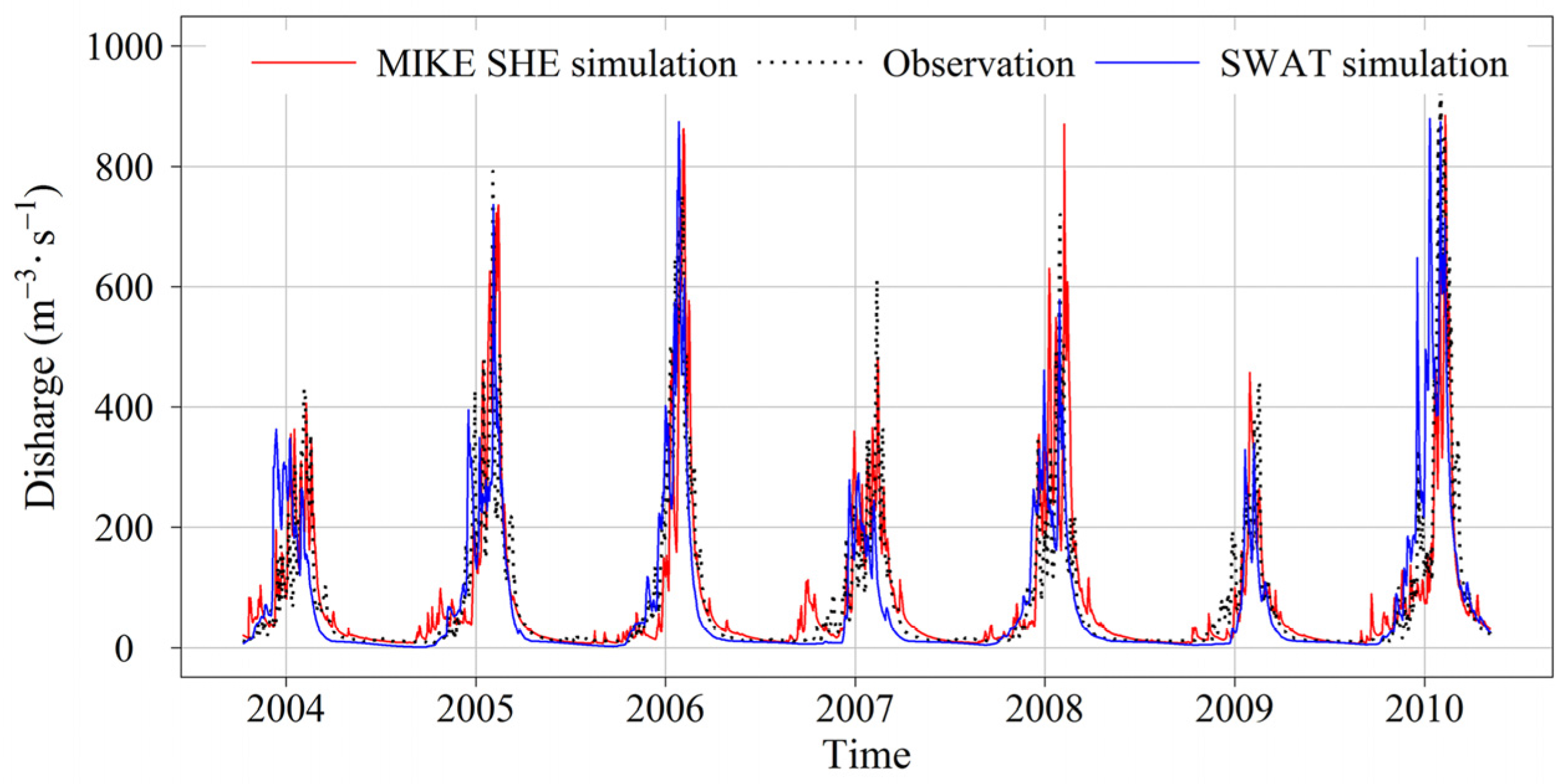
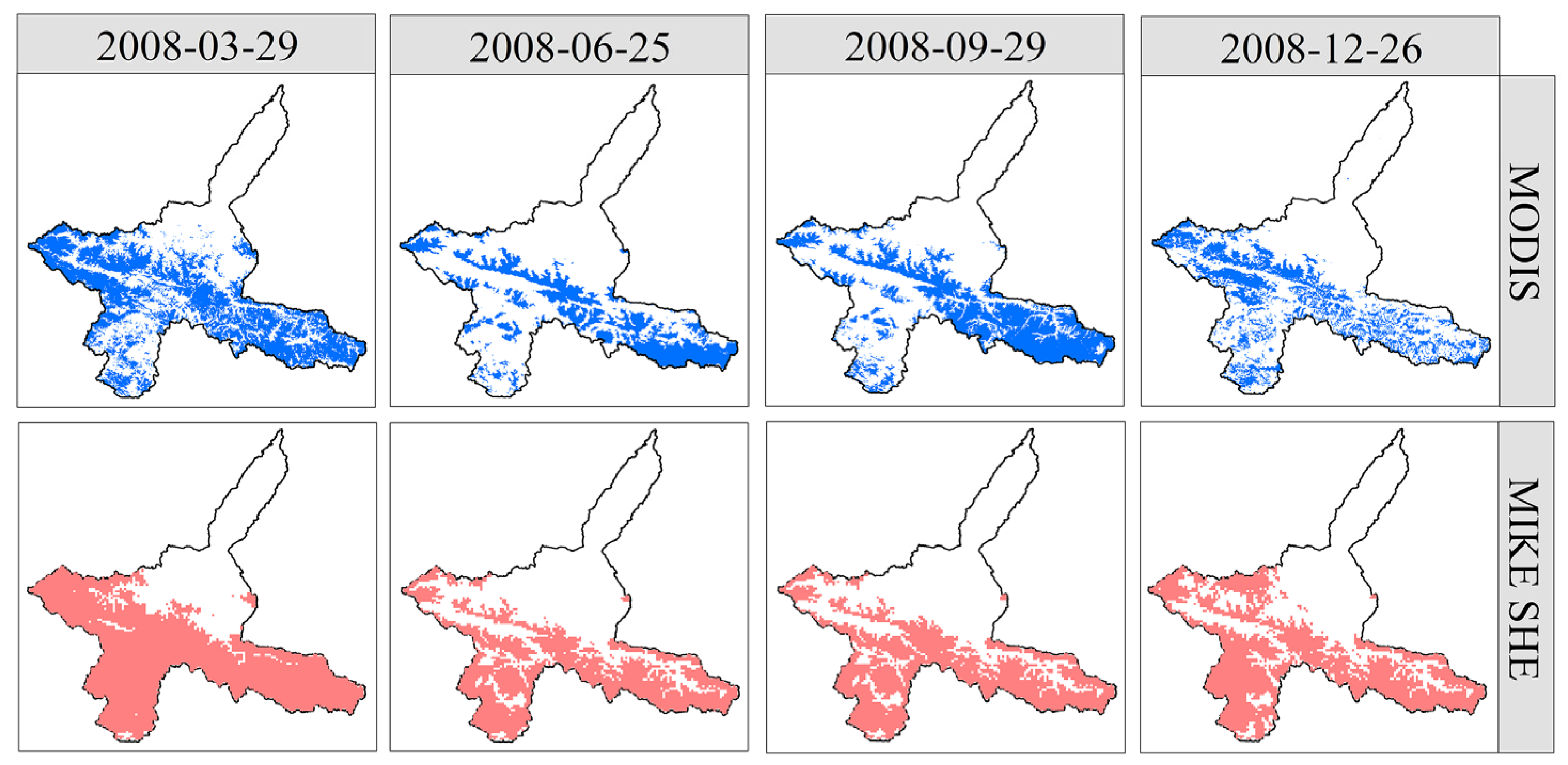
4.1. Results of Hydrological Modelling

The performance of the hydrological models forced by the TRMM rainfall data and other observed meteorological data is shown in Table 1. Both the models simulated conditions quite well, including the results of hydrological simulation for both the calibration (2004–2008) and validation (2009–2010) periods. The results showed that the SWAT model generated good statistical results at a daily time scale (R2, 0.85; NS, 0.71) for calibration and similarly for the validation period (R2, 0.87; NS, 0.76). In addition, the MIKE SHE model provided similar results for calibration (R2, 0.82; NS, 0.66) and validation (R2, 0.89; NS, 0.62). RE for both models was less than 20%. The simulations also captured the peak and low flows as well at a daily time scale (Figure 2), which provided opportunities for an analysis of the effects of climate change on extreme conditions [23]. Both model simulations showed excellent performance with high R2 (over 0.9) and NS (over 0.8) values for the monthly time step. As can be verified from the statistical results, the simulated results from SWAT and MIKE were accepted at both daily and monthly time scales. This study also indirectly shows that TRMM rainfall data can used for both models instead of the ground-based observational data.
When considering that snow cover plays very important role in the study area, the MODIS 10A2 snow cover data and MIKE SHE-modelled snow cover were also compared in our study (Figure 3). Results from four spatial time points in different seasons in 2008 were calculated. The spatial time points from the four seasons in a year are likely to reflect the accumulating and melting processes very well. The following statistical analysis was adopted to evaluate the similarity of the snow cover areas [82]:
U c = A m d A r s A m d A r s ,
where A m d is snow cover area from the MIKE SHE-modelled result, and A r s is the snow cover area from the MODIS 10A2 data. In this research, the U c correlation indicators of the four time points were 0.93, 0.62, 0.77 and 0.67. The similarity between MODIS snow cover and modelled results demonstrated that the MIKE SHE model is able to present the spatial and temporal distribution of snow cover adequately.

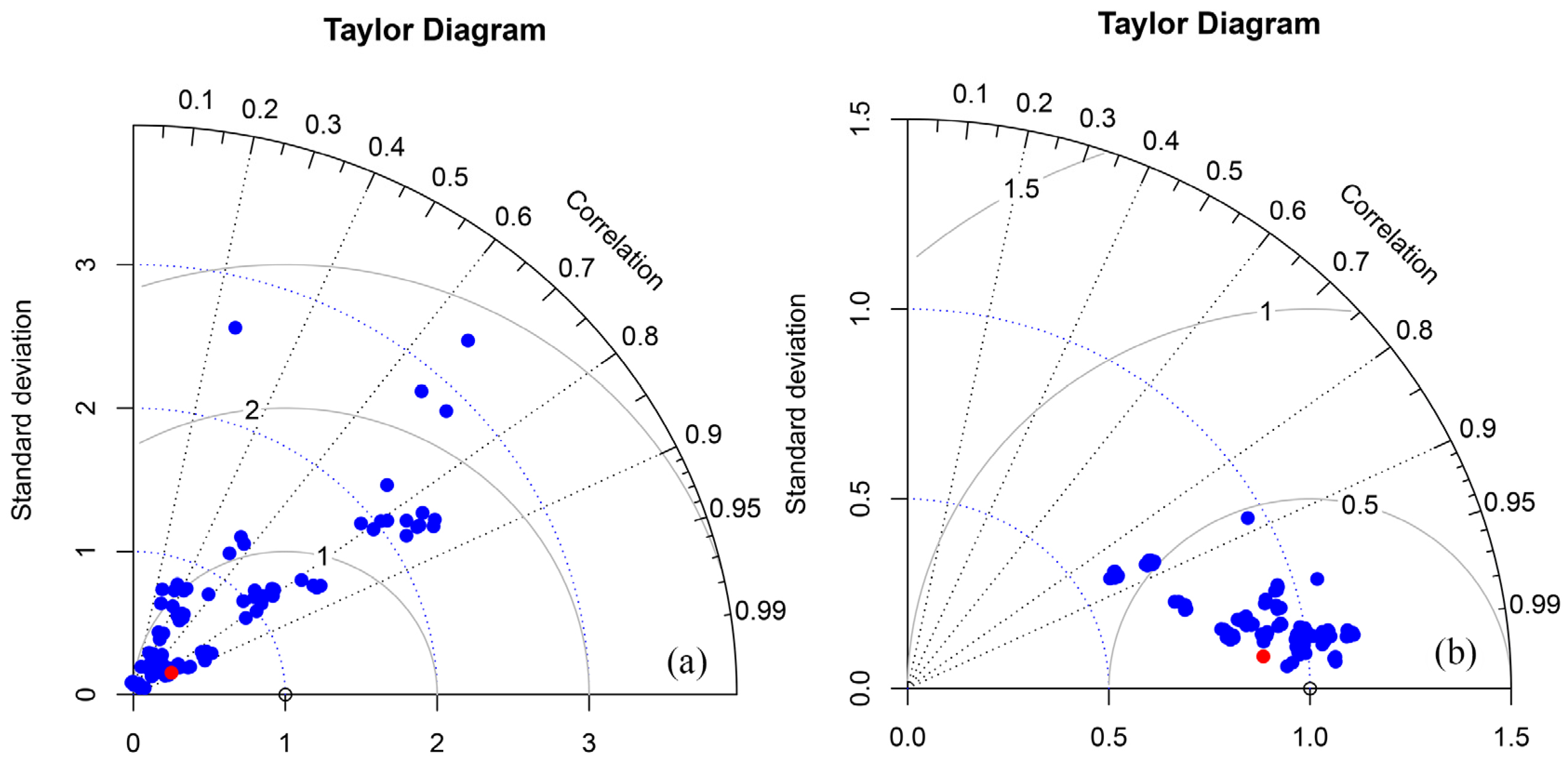
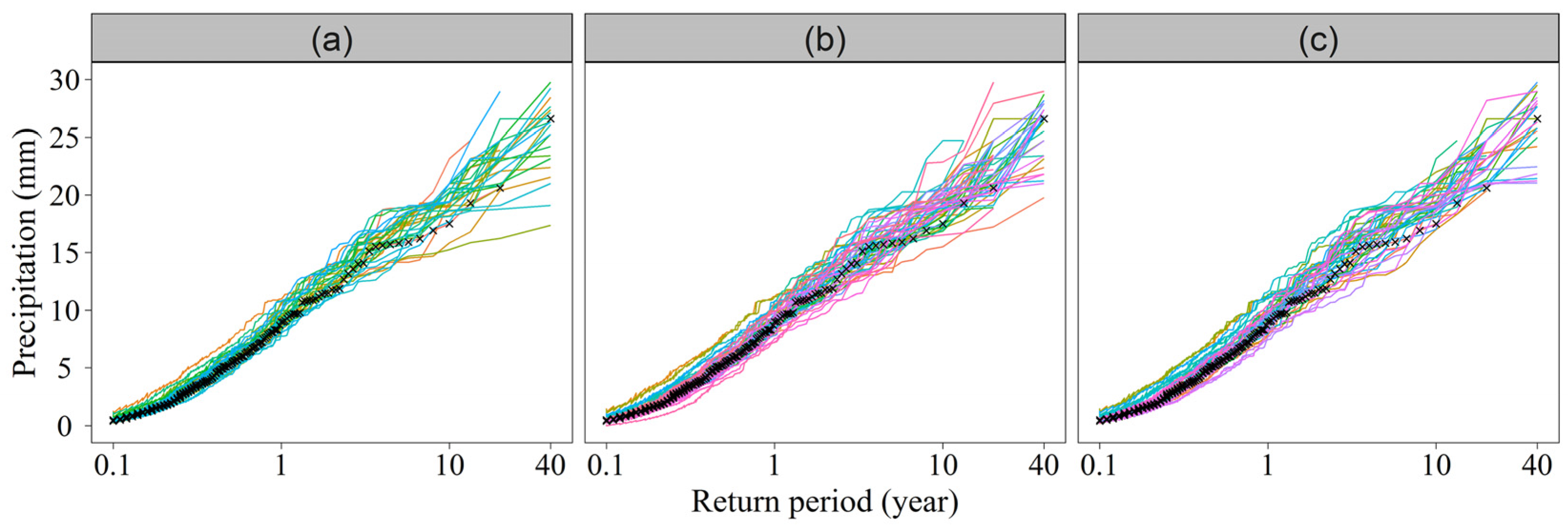
4.2. The Performance of Each GCM Run

Figure 4 shows the precipitation and mean temperature modelling performance for each GCM model simulation and Delta results at a monthly scale during the period of 1965–2004. Only the results from HT station were shown for the purpose of demonstration (Figure 4). Each of the blue points in this figure represents a single GCM run, and the red points represent the Delta results. We can conclude that the Delta results are more representative than most of the GCM runs, and the performance of temperature was much better than that of precipitation (Figure 4). Similar results were also provided by Fang et al. [83] in the Kaidu River Basin and Bokke et al. [84] in the Nile River Basin. The results demonstrate that the precipitation uncertainty is larger than temperature uncertainty in GCMs [85]. For precipitation, most of the GCM runs still exhibited weak performance with correlation coefficients mainly ranging between ca. 0.2–0.8. The results after Delta downscaling was applied could improve the correlation performance, with a value of 0.89. For the projected monthly mean temperature, the GCM runs had a relatively higher correlation with observed data. Most of the correlations between GCM runs and observations were greater than 0.9. After Delta approach downscaling, the correlation between the results and observations was ca. 0.99. Maximum and minimum temperatures have similar precision with average temperature as well. The Delta results for both precipitation and temperature provided more reasonable outcomes for climate change and highlighted the need for a multi-model ensemble approach if researchers are to understand regional climate change [85]. According to the performance of the models, the GCM runs that performed poorly (correlation coefficient of less than 0.4) would not be applied for downscaling processes in precipitation. However, for temperature, the GCM runs with correlations of less than 0.9 would be filtered out.

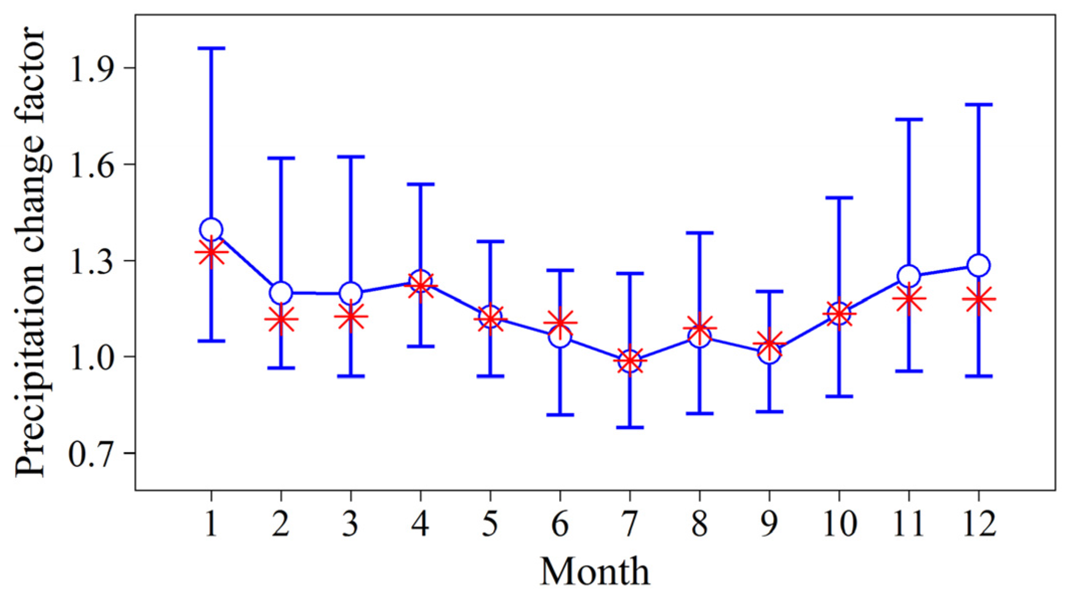
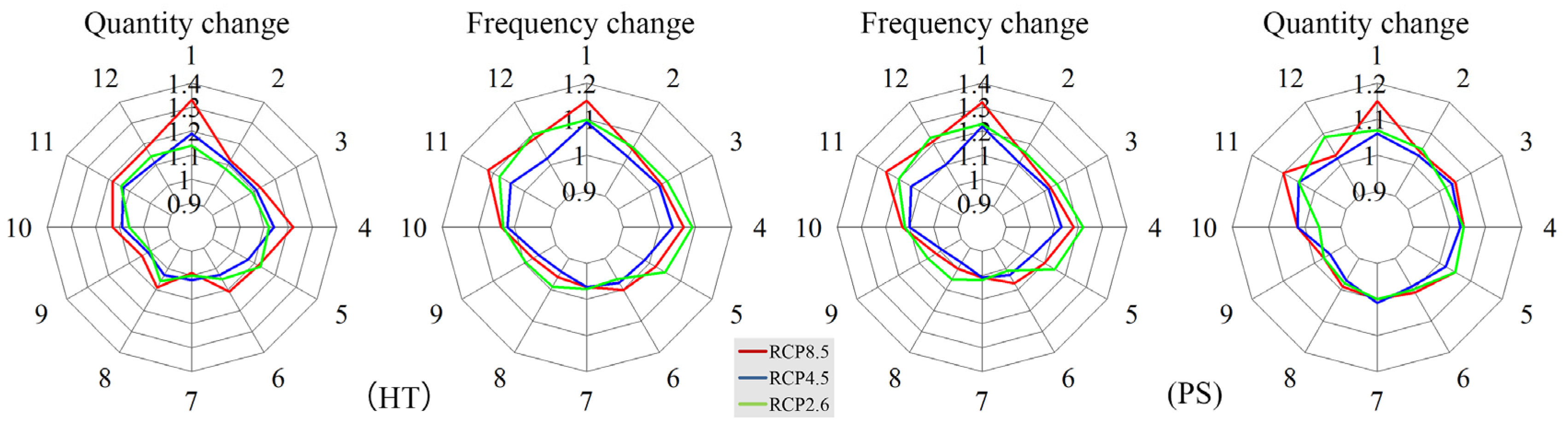
4.3. Precipitation and Temperature Trends

Results from the comparison between wetQPM and Delta were used to validate the wetQPM results. The difference between these two methods was small with −2.59% bias and Std of 4.99% (Figure 5). Similar changes in precipitation intensity were observed for the two methods with a deceasing trend in August and increasing trends in the remaining months, which included an increase of up to 30% in winter. The wetQPM predictions were always restricted between the maximum and minimum changes calculated by the GCMs models, which also indirectly demonstrated the reasonability of the wetQPM. The results between the two methods had few differences, and wetQPM, which considered both precipitation frequency and totals was more representative than the Delta method, which accounted only for measures of total precipitation. The wetQPM results were assumed to have higher precision, and they were used and selected for future analysis of the effects of climate change.
Figure 6 shows that the multi-model median in perturbation factors of monthly precipitation intensity and frequency that were calculated by wetQPM at the HT and PS stations. When the change factor was equal to 1, this only indicated that future precipitation would have no change when compared with the historical period [23]. The modeled results of precipitation show it will increase overall both at HT and PS stations during the dry season from November to March, which is a relatively higher change than in the wet season from April to October. Only in the summer months of July and August for different scenarios did the precipitation decreased slightly by ca. −0.4% to −3.1% (Table 2), which was the same as results previously observed for different arid and semi-arid regions of the Kaidu River [83], Zarqa River [86] and Colorado River [87] basins. Meanwhile, heavier rainfall events and more dry days might occur in late summer and early autumn when considering that precipitation would have an increasing trend in intensity but decreasing in frequency. These results also agreed with the results provided by Figure 7 that represent the observed quantiles versus simulations of the GCM scenarios. From the three scenario results (Figure 7), a comparatively higher absolute amount of variability in future rainfall was projected for extremes than for observations during most GCM runs. This phenomenon illustrated that more extreme rainfall events will occur in the near future; the results also agree quite well with the IPCC AR5 results that demonstrated an increasing trend in heavy rainfall in the future [3]. When the three RCPs emission scenarios were compared, the RCP8.5 scenario indicated relatively higher perturbation factors than RCP2.6 and RCP4.5, particularly at HT station.
Delta method projections at HT and PS stations showed a significant change in monthly average temperature was predicted to occur in the near future (Figure 8, Table 2). Projected monthly average temperature will increase from 1.60 to 2.61 °C and 1.66 to 2.58 °C for HT and PS stations, respectively, under the three future climate scenarios. The results of the RCP8.5 scenario show an apparent higher increase than RCP2.6 and RCP4.5 with increasing temperature always higher than 2 °C. This was also confirmed by the conclusions drawn for the IPCC AR5 as mentioned earlier [3]. When focusing on the different seasons, the mean monthly temperature increase was higher in summer and winter when compared with spring and autumn. The projected minimum temperature (Tmin) increased slightly in summer and autumn when compared with the maximum temperature (Tmax) in winter and spring, which indicated warmer nights would occur in spring and winter. However, the projected Tmin increased at a lower rate than Tmax, which demonstrates that greater warming is expected to occur during the daytime in summer and autumn.

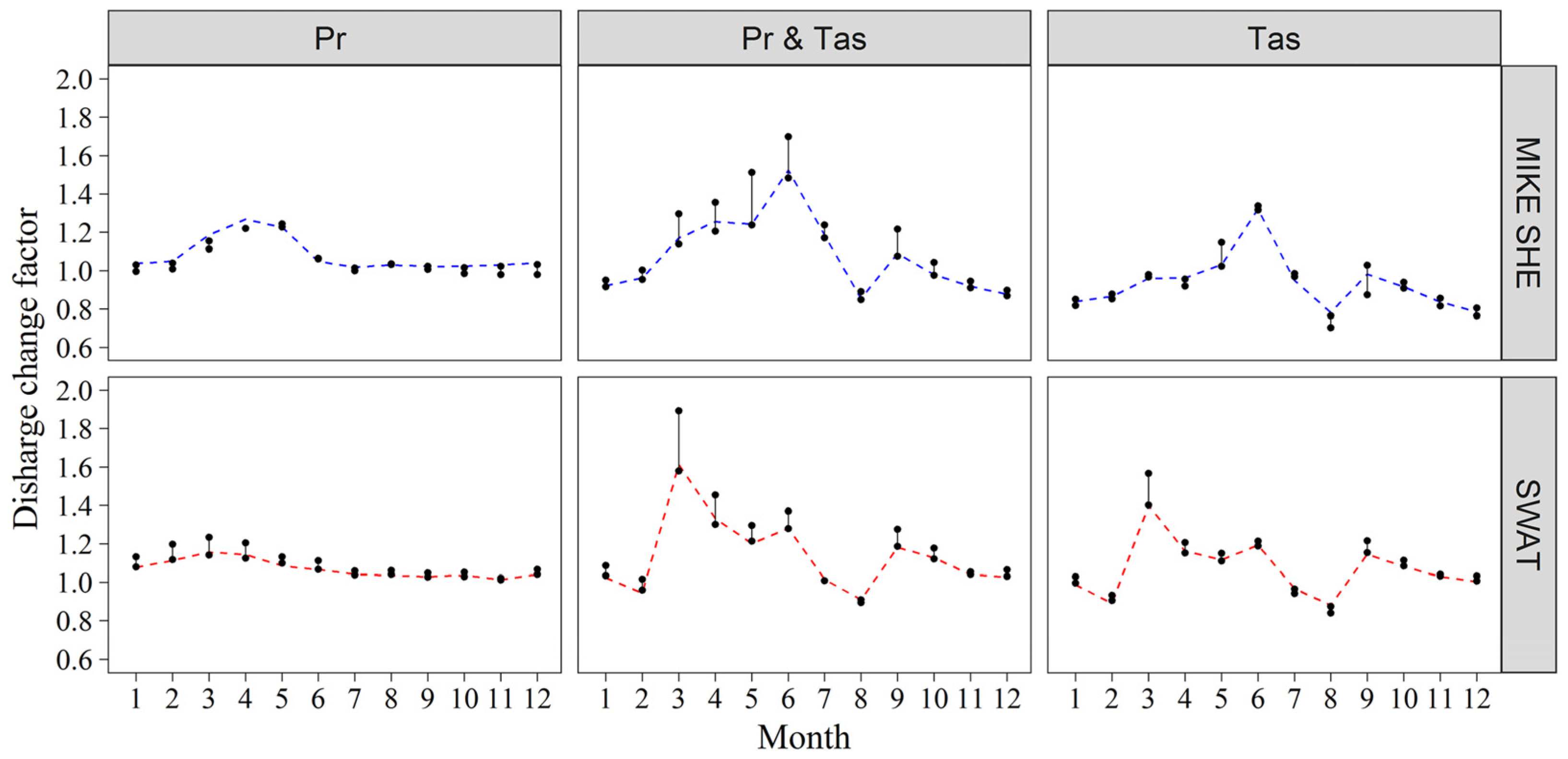
4.4. The Combined Effects of Both Precipitation and Temperature Input Variables

The second row in Figure 9 shows the mean level of the effects on the average monthly flow at the Tongguziluoke (TGZLK) gauging station. Clear seasonal variability was demonstrated in the flow changes. From the MIKE SHE results, the flow changes strongly increase during spring (March to May; 17.1–25.5%). The effects based on the SWAT results were even more strongly positive, and as high as 61.3% for March. The results of both models indicated the effects caused the snowmelt period to become longer and occur earlier. In summer, a relatively larger increase (18.6–52.2%) was found during June–July for the MIKE SHE model, while the SWAT model also demonstrated an increasing trend of 1.5–28.1%. In August, both the MIKE SHE and SWAT models predicted a decreasing trend with rates of −14.5% and −9.1%, respectively. This could be the result of the dual functions of precipitation and less snowmelt. For autumn and winter, the situation was very different. The MIKE SHE showed an increase during September and a decreasing trend for other months of −2% to −12.4%. For SWAT results, the flow was always predicted to increase from September to January (2.6–18.2%) and slightly decrease (−5.7%) in February.
When considering that the accumulation and melting of glaciers and snow are important in an arid alpine basin, Figure 10 establishes the changes in glaciers and snowmelt under three future scenarios. It is worth pointing out that both models calculate the ice melting by using a simplified degree-day approach. In this case, the ice and snow melting processes were simulated by the same equation. Fortunately, the simplified approach is able to represent the snow and ice melting processes reasonably. MIKE SHE modelled over a longer snowmelt period with more dispersed temporal distribution than SWAT. The SWAT model applies the variation of a snowmelt factor and snow pack temperature that reflects the accumulated temperature of the land surface while only air temperature is considered in MIKE SHE. According to findings provided by Liu et al. [88], this is the possible reason from the resulting snowmelt difference in these two models. An advance in the snowmelt period leads to much less snowmelt in July and August in the SWAT model, which may cripple the flood peak in summer. For MIKE SHE, the snowmelt only decreased slightly in August, which implied that the flood peak would be relatively less affected by the earlier snowmelt season. Simultaneously, May will change from a month of snow accumulation to a month of snowmelt according to the snow storage change.
The MIKE SHE model also provides information about the spatial distribution of the hydrological variables. Figure 11 reveals the spatial distribution of snow storage on August 31 of the last year in simulation as well as in each scenario. According to the MIKE SHE distributed results, most of the middle and high mountainous areas are covered with snow, which accounts for 32.5% of the entire research area. In future scenarios, the snowpack area shrinks sharply in the middle of the mountainous area with the proportion only occupying 11.9%, which illustrates the increased elevation of the snowline and decrease in snow covered area and water storage as snow. As supplemental evidence, Figure 12 shows the distribution of snow-covered areas in the different elevation bands. The snowline will shift upward ca. 200 m because of disappearing of accumulated snow between 4.0–4.2 km in elevation. The accumulated snow at elevations between 4.2–6.4 km will also decline under all three scenarios. However, when the elevation exceeds 6.4 km, the snow accumulation will increase sustainably. The rising temperatures scarcely influence the snow storage at this elevation considering the increased temperature barely reached the critical snowmelt temperature.
The effects on daily average discharges, as well as on daily peak and low flow extremes were also analyzed (Figure 13). For total flow at the TGZLK station, the SWAT results simulated a larger increase of 6.5%, 7.1% and 10.5% when compared with the MIKE SHE model (0.9%, 2.5% and 10%) under the RCP2.6, RCP4.5 and RCP8.5 scenarios, respectively. Similar findings were also simulated for low flow. However, the two models present a dramatic discrepancy when the peak flow results are compared. For MIKE SHE results, the peak flow always increased and ranged from 9.1% to 13.9%, while the simulated peak flow decreased based on the SWAT model (−20.9% to −24.4%). The peak flow mainly occurs in summer when there is a large amount of snow and ice melt. Therefore, the differences in ice-snow melting process and snow cover distributions affect the formation of peak flow in both models.Primarily, most of the ice-snow melt water infiltrates into the soil and contributes to stream runoff as subsurface runoff [89,90] in the SWAT model. In the MIKE SHE model, however, the soil lateral flow is ignored [88]. The infiltrated soil water could flow back to the surface when the head pressure of aquifer water is higher than at the surface [91]. Therefore, the peak flow response are slowed in SWAT. In addition, the spatial distribution of snow pack is homogeneous at the sub-basin scale in the SWAT model. However, each grid can reflect the actual spatial change of the snow storage in the fully distributed MIKE SHE model. Therefore, the MIKE SHE model is expected to provide more representative results than the SWAT model in terms of simulating the peak flow in this study.
The response of evapotranspiration to predicted climate change is demonstrated in Figure 14. The two models predicted fairly similar changes in evapotranspiration. Evapotranspiration changes were always positive for all seasons with relatively higher increases occurring in summer. The results also showed that evapotranspiration was more sensitive to temperature when compared with precipitation. When different emission scenarios were compared, the RCP8.5 scenario also had a clearly higher change factor than the RCP2.6 and RCP4.5 scenarios. The increased evapotranspiration rates for low and median scenarios ranged from 7.6–27.7% and 7.8–24.4% in the MIKE SHE and SWAT models, respectively. When focusing on the high scenario, the increased rates of evapotranspiration were 9.4–31.1% and 8.9–31.3% in MIKE SHE and SWAT models, respectively.

4.5. The Separate Effects of Precipitation and Temperature

For evaluating the sensitivity of water resources to changes in climatic factors for different hydrological models, the simulated effects from changes in a single climatic factor were also estimated by applying both hydrological models to changes in precipitation and temperature separately. For both models, the simulated increases in precipitation also resulted in an increase in the discharge rate (Q) (Figure 9, 1st row). However, for temperature, the situation was very different. The sensitivity of discharge to temperature was heterogeneous in different seasons considering the dependence of discharge on snowmelt (Figure 9, 3rd row). In general, Q was positively related to an increase in temperature in the SWAT model, while Q was negatively related to temperature in the MIKE SHE model on an annual scale (Table 3). A previous study showed that the proportion of melting glacial water and snow in the total discharge was approximately 66.8% [92]. Therefore, the discharge was more sensitive to temperature when compared with precipitation; this also has been documented in many other places [59,93,94]. In fact, for the MIKE SHE model, the ratio of δ Q/ δ P increases from 0.8 to 1.29 with an increase of δ P. This occurs because the larger δ P accounts for more Q when the temperature remained unchanged. A larger decrease in discharge was also found with a relatively higher Δ Tas. A 1 °C change in temperature led to −3.64%, −3.96% and −4.52% changes in discharge under RCP2.6, RCP4.5 and RCP8.5, respectively. However, for the SWAT model, the δ Q/ δ P remained almost consistent in different scenarios at ca. 0.73. The δ Q/ Δ Tmax ( δ Q/ Δ Tmin) initially increased and then decreased with an increase in Δ Tmax ( Δ Tmin), which also indicates that the increased discharge will level out and even tend to decrease with constant increases in temperature. Meanwhile, the discharge had higher sensitivity to temperature and precipitation in the MIKE SHE when compared with the SWAT model with a higher absolute δ Q/ δ P and δ Q/ Δ T.

5. Conclusions

The present study predicted the possible effects of climate change on water resources in the ungauged Hotan River Basin by the application of remote sensing data and climate change data. Two statistical downscaling (SD) methods, i.e., the WetQPM and Delta approaches, were compared and used to extract the climate change signals for the period of 2021–2060 while using 1965–2004 as a control. Coupled with two hydrological models, the fully distributed MIKE SHE model and the semi-distributed SWAT model, in responses of discharge, extreme events, evapotranspiration, and snowmelt and snow accumulation, were evaluated with the effects of changing climate. The main conclusions are summarized as follows:
(1)
Based on the statistical evaluation indices of discharge calibration as well as validation at TGZLK station, both the MIKE SHE and SWAT models demonstrated acceptable performance in the Hotan River Basin when driven by TRMM daily rainfall data.
(2)
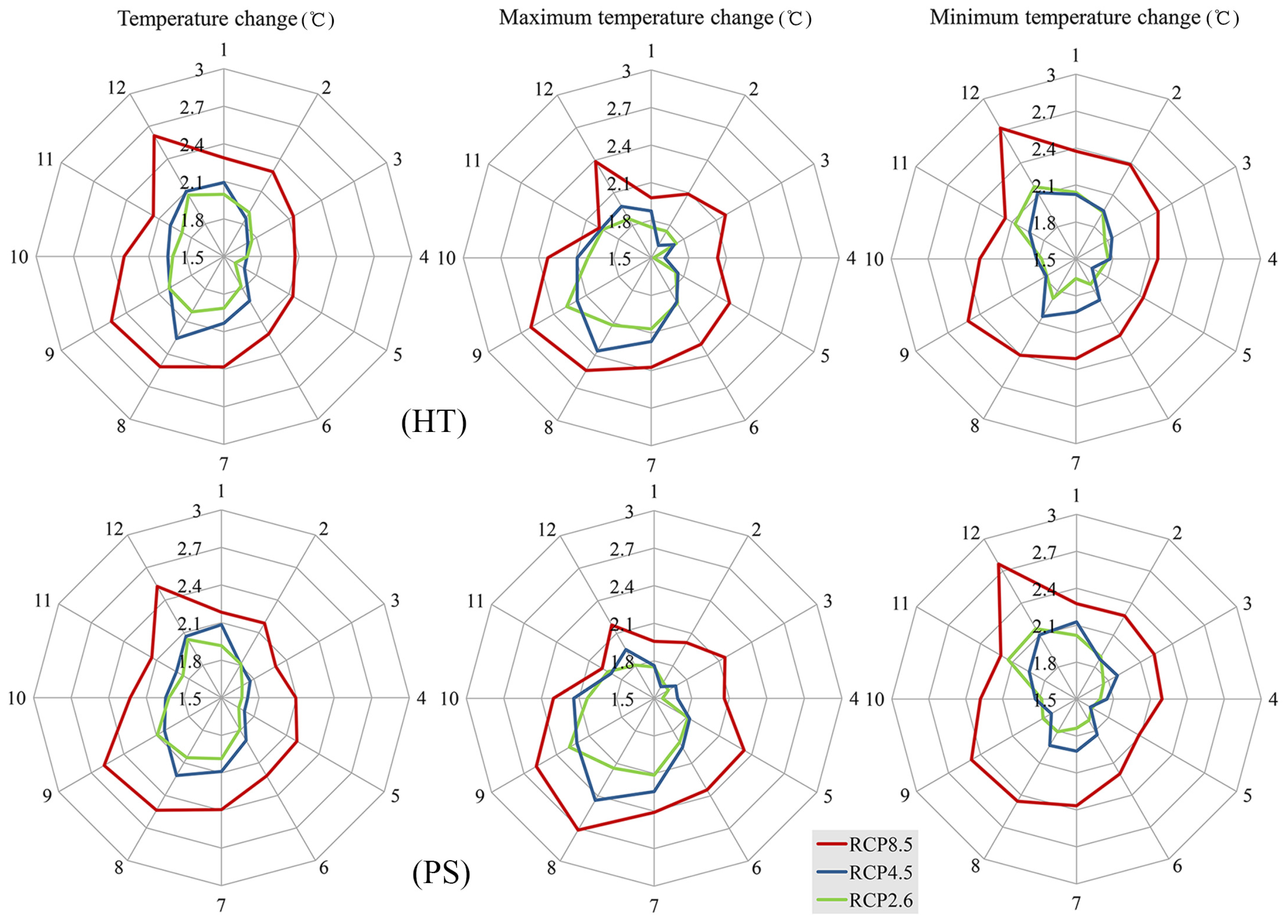
The precipitation is projected to experience an overall increase with rates ranging between −1.2% to 32.7% (−3.1% to 31.8%) at HT (PS) station. The dry season is predicted to have relatively higher increases than the wet season while a slightly decreasing trend was predicted for July (August and September). The projected average temperature was expected to increase by 1.60–2.61 °C (1.66–2.58 °C) at HT (PS) station. The projected Tmax increased slightly more when compared with Tmin during summer and autumn, which represents the predicted warmer daytime temperatures.
(3)
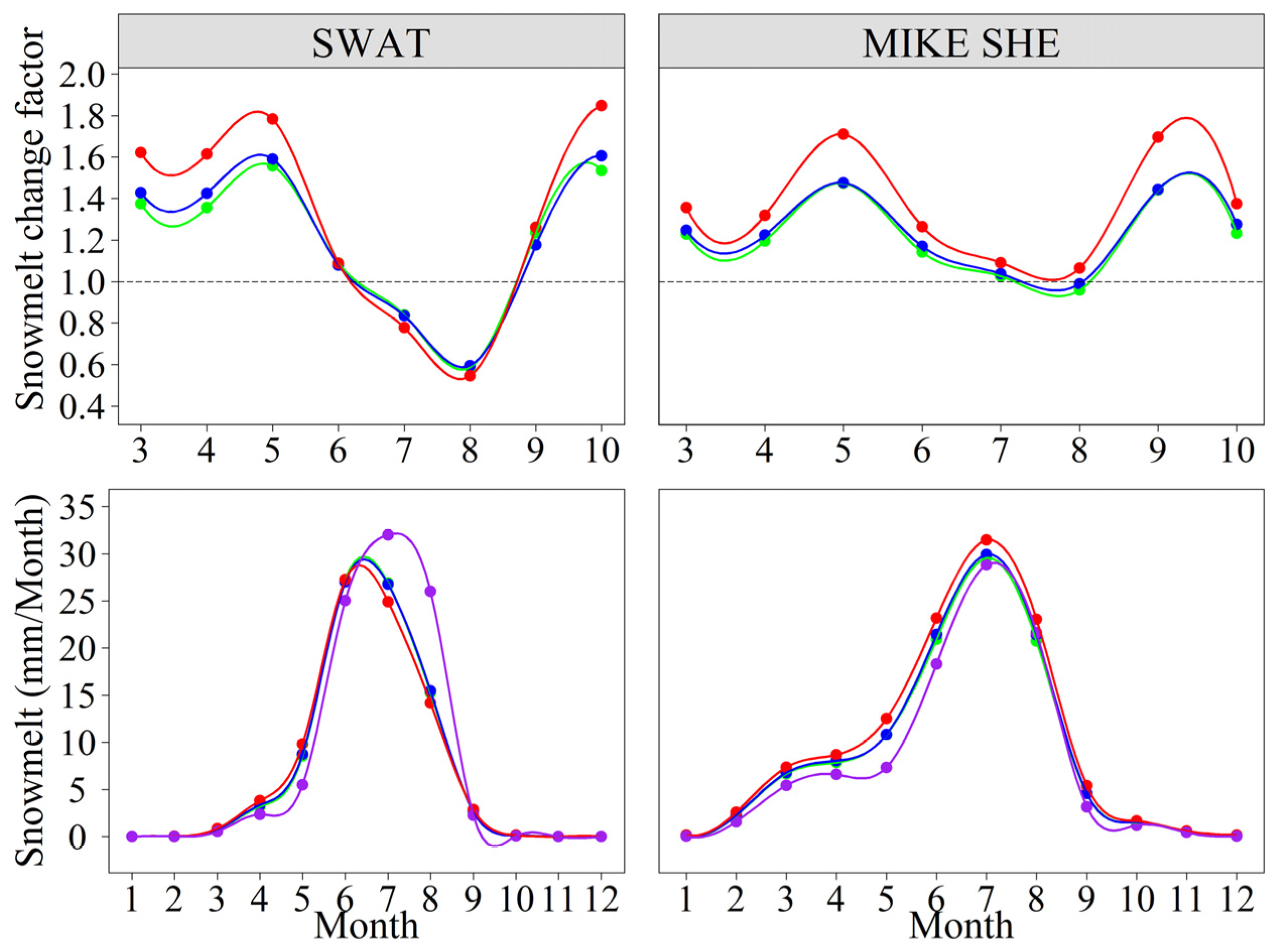
The structure of the hydrological models strongly influences the simulated effects of climate change. MIKE SHE model was found to be more sensitive to simulated precipitation as well as temperature than the SWAT model. Discharge will increase with an increase of precipitation in both models. With an increase in temperature, the discharge significantly decreased in the MIKE SHE model, while it increased in the SWAT model. However, the increase in magnitude became smaller and even tended to decrease with a sustained increase in temperature.
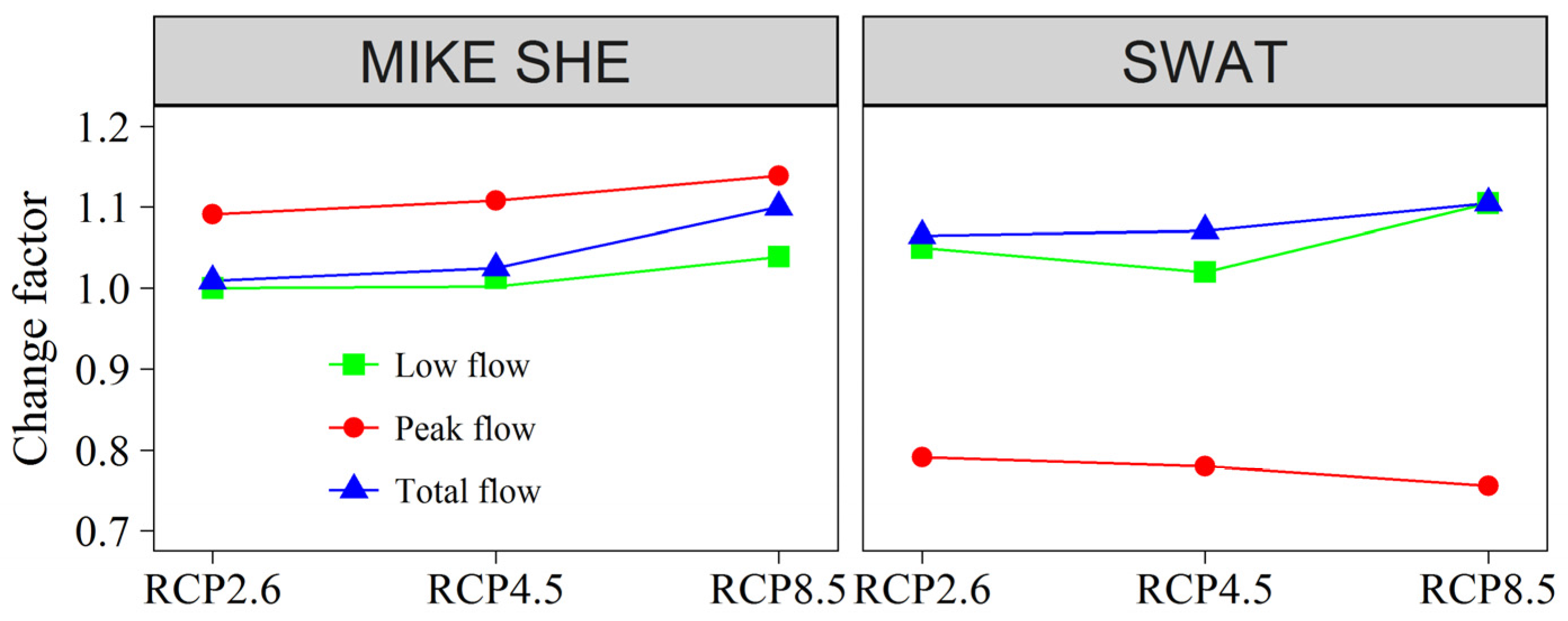
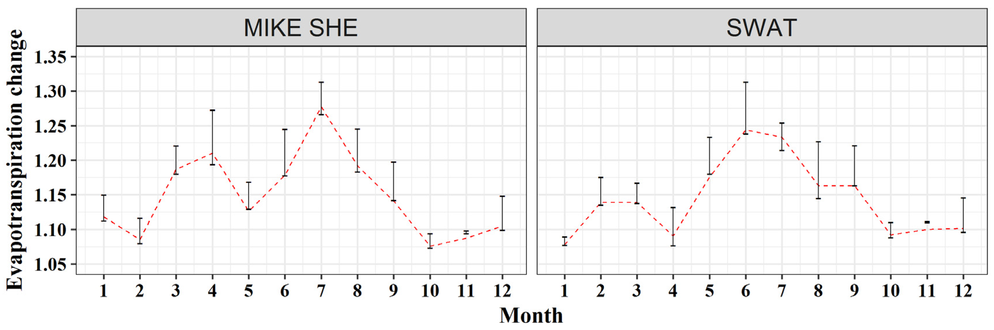
(4)
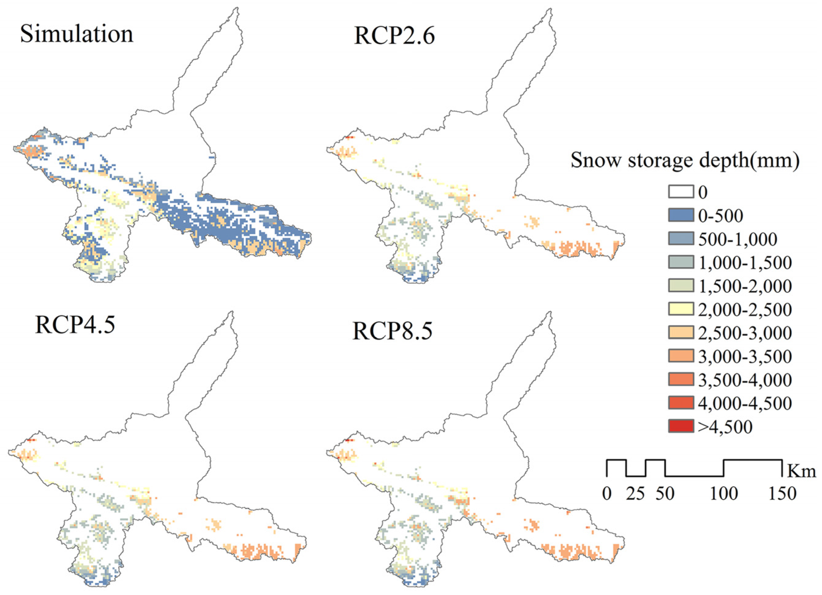
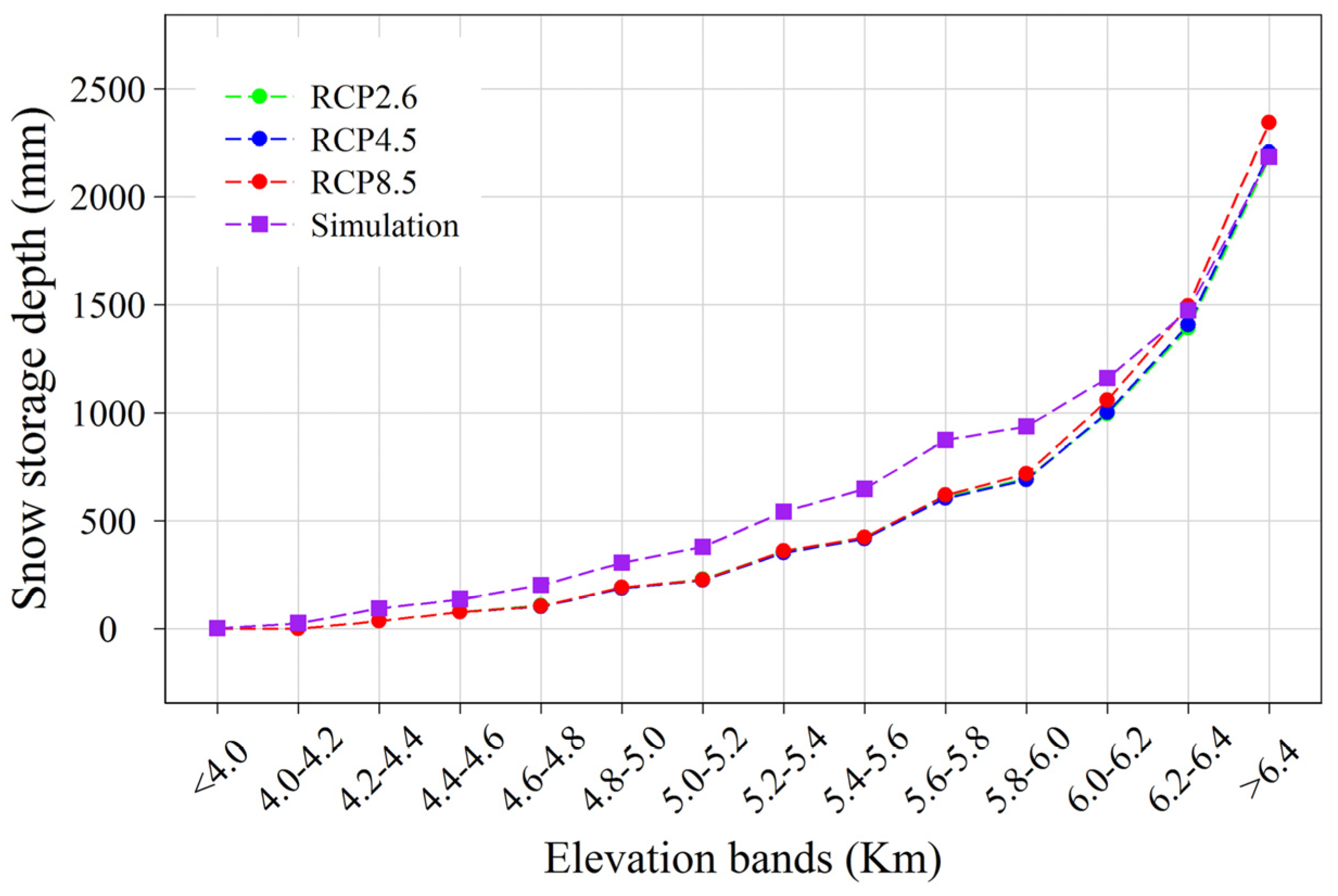
The snowline was predicted to increase in elevation by ca. 200 m with a loss of accumulated snow at 4.2–6.2 km elevation. The evapotranspiration rate will increase significantly by 7.4% to 31.3%. Climate change is predicted to lead to stronger changes in peak flow than in the total and low flow. The semi-distributed SWAT model has obvious limitations when focusing on the peak flow response to climate change when compared with the MIKE SHE model.
Stream flow is generally predicted to increase, while the shrinking of snow storage and a reduction in the snowpack will sharply reduce the solid water storage (snow storage) capacity of the landscape. This proves that a growth in water resources is unsustainable. The increasing frequency of extreme events and a spatiotemporal redistribution of water resources will also produce great challenges related to agricultural water allocation and management in this region. It is worth pointing out that the accumulating and melting processes of glaciers were calculated by the degree-day approach. Both models used the same equation to simulate the melting of snow and glaciers. Therefore, the response of glaciers to climate change was not included in this study. Modifying model structures and adding the special glacier module would dramatically improve the reliability of hydrological models in catchments in the future work. Meanwhile, the effects of climate change are strongly controlled by the hydrological model structure from the application of the MIKE SHE and SWAT models. Therefore, the joint application of multiple hydrological models and combined results could be an effective way to improve our understanding the effects of climate change on water resources. The application of remote sensing data and climate change data provides a new method to that can be used to predict the effects of climate change in remote ungauged regions, which is of great significance and is related to creating new water resource management guidelines and planning schemes for local people and decision makers.

Acknowledgments

This work was supported by the “Thousand Youth Talents Plan” (Xinjiang Project No.374231001), the International Partnership Program of the Chinese Academy of Sciences (Grant No. 131551KYSB20160002), the key research program of the Chinese Academy of Sciences (CAS) (Grant No. KZZD-EW-12-3), the Project of the Chinese Academy of Sciences (Grant No. Y674122) and the International Cooperation Training Program of Innovative Talent in 2016, China Scholarship Council (Grant No. 201604910973) and Sino-Belgian Personnel Training Program for Geo-information. Data for this work were provided through the IPCC Data Distribution Center and through the China Meteorological Data Sharing Service System. The IPCC data are available for download from http://www.ipcc-data.org/ and the observed meteorological data from http://cdc.cma.gov.cn/home.do.

Author Contributions

Tie Liu, Amaury Frankl and Philippe De Maeyer conceived and designed the experiments of this study; Min Luo, Fanhao Meng, Alishir Kurban and Yongchao Duan collected and processed the data; Min Luo, Yongchao Duan and Fanhao Meng calibrated and validated the model; Min Luo analysed the results and wrote the paper. All authors have proofread and approved the final manuscript.

Conflicts of Interest

The authors declare that there is no conflict of interest regarding the publication of this paper.

References

  1. Pall, P.; Aina, T.; Stone, D.A.; Stott, P.A.; Nozawa, T.; Hilberts, A.G.; Lohmann, D.; Allen, M.R. Anthropogenic greenhouse gas contribution to flood risk in England and Wales in autumn 2000. Nature 2011, 470, 382–385. [Google Scholar] [CrossRef] [PubMed]
  2. Carter, J.G.; Cavan, G.; Connelly, A.; Guy, S.; Handley, J.; Kazmierczak, A. Climate change and the city: Building capacity for urban adaptation. Prog. Plan. 2015, 95, 1–66. [Google Scholar] [CrossRef] [Green Version]
  3. IPCC. Climate Change 2013: The Physical Science Basis. Contribution of Working Group I to the Fifth Assessment Report of the Intergovernmental Panel on Climate Change; Stocker, T.F., Qin, D., Plattner, G.-K., Tignor, M., Allen, S.K., Boschung, J., Nauels, A., Xia, Y., Bex, V., Midgley, P.M., Eds.; Cambridge University Press: Cambridge, UK, 2013. [Google Scholar]
  4. Abbaspour, K.C.; Faramarzi, M.; Ghasemi, S.S.; Yang, H. Assessing the impact of climate change on water resources in Iran. Water Resour. Res. 2009, 45, W10434. [Google Scholar] [CrossRef]
  5. Vicuna, S.; Dracup, J. The evolution of climate change impact studies on hydrology and water resources in California. Clim. Chang. 2007, 82, 327–350. [Google Scholar] [CrossRef]
  6. Liu, Z.; Xu, Z.; Huang, J.; Charles, S.P.; Fu, G. Impacts of climate change on hydrological processes in the headwater catchment of the Tarim River Basin, China. Hydrol. Process. 2010, 24, 196–208. [Google Scholar] [CrossRef]
  7. Wang, B.; Zhang, M.; Wei, J.; Wang, S.; Li, S.; Ma, Q.; Li, X.; Pan, S. Changes in extreme events of temperature and precipitation over Xinjiang, Northwest China, during 1960–2009. Quat. Int. 2013, 298, 141–151. [Google Scholar] [CrossRef]
  8. Ma, Z.; Kang, S.; Zhang, L.; Tong, L.; Su, X. Analysis of impacts of climate variability and human activity on streamflow for a river basin in arid region of Northwest China. J. Hydrol. 2008, 352, 239–249. [Google Scholar] [CrossRef]
  9. Lioubimtseva, E.; Cole, R.; Adams, J.; Kapustin, G. Impacts of climate and land-cover changes in arid lands of Central Asia. J. Arid Environ. 2005, 62, 285–308. [Google Scholar] [CrossRef]
  10. Lioubimtseva, E.; Henebry, G.M. Climate and environmental change in arid Central Asia: Impacts, vulnerability, and adaptations. J. Arid Environ. 2009, 73, 963–977. [Google Scholar] [CrossRef]
  11. Yang, L.; Zhang, Q. Effects of the North Atlantic oscillation on the summer rainfall anomalies in Xinjiang. Chin. J. Atmos. Sci. 2008, 32, 1187–1196. [Google Scholar]
  12. Chen, Y.; Xu, C.; Hao, X.; Li, W.; Chen, Y.; Zhu, C.; Ye, Z. Fifty-year climate change and its effect on annual runoff in the Tarim River Basin, China. Quat. Int. 2009, 208, 53–61. [Google Scholar]
  13. Zhang, Q.; Xu, C.-Y.; Tao, H.; Jiang, T.; Chen, Y.D. Climate changes and their impacts on water resources in the arid regions: A case study of the Tarim River Basin, China. Stoch. Environ. Res. Risk Assess. 2010, 24, 349–358. [Google Scholar] [CrossRef]
  14. Barnett, T.P.; Adam, J.C.; Lettenmaier, D.P. Potential impacts of a warming climate on water availability in snow-dominated regions. Nature 2005, 438, 303–309. [Google Scholar] [CrossRef] [PubMed]
  15. Charlton, R.; Fealy, R.; Moore, S.; Sweeney, J.; Murphy, C. Assessing the impact of climate change on water supply and flood hazard in Ireland using statistical downscaling and hydrological modelling techniques. Clim. Chang. 2006, 74, 475–491. [Google Scholar] [CrossRef]
  16. Steele-Dunne, S.; Lynch, P.; McGrath, R.; Semmler, T.; Wang, S.; Hanafin, J.; Nolan, P. The impacts of climate change on hydrology in Ireland. J. Hydrol. 2008, 356, 28–45. [Google Scholar] [CrossRef]
  17. Hessami, M.; Gachon, P.; Ouarda, T.B.M.J.; St-Hilaire, A. Automated regression-based statistical downscaling tool. Environ. Model. Softw. 2008, 23, 813–834. [Google Scholar] [CrossRef]
  18. Ahmed, K.F.; Wang, G.; Silander, J.; Wilson, A.M.; Allen, J.M.; Horton, R.; Anyah, R. Statistical downscaling and bias correction of climate model outputs for climate change impact assessment in the US Northeast. Glob. Planet. Chang. 2013, 100, 320–332. [Google Scholar] [CrossRef]
  19. Ouyang, F.; Lü, H.; Zhu, Y.; Zhang, J.; Yu, Z.; Chen, X.; Li, M. Uncertainty analysis of downscaling methods in assessing the influence of climate change on hydrology. Stoch. Environ. Res. Risk Assess. 2014, 28, 991–1010. [Google Scholar] [CrossRef]
  20. Xu, C.Y. Climate change and hydrologic models: A review of existing gaps and recent research developments. Water Resour. Manag. 1999, 13, 369–382. [Google Scholar] [CrossRef]
  21. Hassan, Z.; Shamsudin, S.; Harun, S. Application of sdsm and lars-wg for simulating and downscaling of rainfall and temperature. Theor. Appl. Climatol. 2013, 116, 243–257. [Google Scholar] [CrossRef]
  22. Mahmood, R.; Jia, S. An extended linear scaling method for downscaling temperature and its implication in the Jhelum River Basin, Pakistan, and India, using CMIP5 GCMs. Theor. Appl. Climatol. 2016. [Google Scholar] [CrossRef]
  23. Liu, T.; Willems, P.; Pan, X.; Bao, A.M.; Chen, X.; Veroustraete, F.; Dong, Q. Climate change impact on water resource extremes in a headwater region of the Tarim Basin in China. Hydrol. Earth Syst. Sci. 2011, 15, 6593–6637. [Google Scholar] [CrossRef]
  24. Liu, J.; Luo, M.; Liu, T.; Bao, A.; De Maeyer, P.; Feng, X.; Chen, X. Local climate change and the impacts on hydrological processes in an arid alpine catchment in Karakoram. Water 2017, 9, 344. [Google Scholar] [CrossRef]
  25. Onyutha, C.; Tabari, H.; Rutkowska, A.; Nyeko-Ogiramoi, P.; Willems, P. Comparison of different statistical downscaling methods for climate change rainfall projections over the Lake Victoria Basin considering CMIP3 and CMIP5. J. Hydro-Environ. Res. 2016, 12, 31–45. [Google Scholar] [CrossRef]
  26. Miles, E.L.; Elsner, M.M.; Littell, J.S.; Binder, L.W.; Lettenmaier, D.P. Assessing regional impacts and adaptation strategies for climate change: The Washington climate change impacts assessment. Clim. Chang. 2010, 102, 9–27. [Google Scholar] [CrossRef]
  27. Wilby, R.L.; Hay, L.E.; Gutowski, W.J.; Arritt, R.W.; Takle, E.S.; Pan, Z.; Leavesley, G.H.; Clark, M.P. Hydrological responses to dynamically and statistically downscaled climate model output. Geophys. Res. Lett. 2000, 27, 1199–1202. [Google Scholar] [CrossRef]
  28. Nyeko-Ogiramoi, P.; Willems, P.; Ngirane-Katashaya, G.; Ntegeka, V. Nonparametric statistical downscaling of precipitation from global climate models. In Climate Models; InTech Europe, University Campus STeP Ri.: Slavka Krautzeka, Croatia, 2012; pp. 109–136. [Google Scholar]
  29. Liu, J.; Liu, T.; Bao, A.; De Maeyer, P.; Kurban, A.; Chen, X. Response of hydrological processes to input data in high alpine catchment: An assessment of the Yarkant River Basin in China. Water 2016, 8, 181. [Google Scholar] [CrossRef]
  30. Huang, Y.; Chen, X.; Bao, A.; Ma, Y. Distributed hydrological modeling in Kaidu Basin: MIKE-SHE model calibration and uncertainty estimation. J. Glaciol. Geocryol. 2010, 32, 567–572. [Google Scholar]
  31. Deus, D.; Gloaguen, R.; Krause, P. Water balance modeling in a semi-arid environment with limited in situ data using remote sensing in Lake Manyara, East African Rift, Tanzania. Remote Sens. 2013, 5, 1651–1680. [Google Scholar] [CrossRef]
  32. Ushio, T.; Sasashige, K.; Kubota, T.; Shige, S.; Okamoto, K.I.; Aonashi, K.; Inoue, T.; Takahashi, N.; Iguchi, T.; Kachi, M. A kalman filter approach to the global satellite mapping of precipitation (GSMAP) from combined passive microwave and infrared radiometric data. J. Meteorol. Soc. Jpn. Ser. II 2009, 87, 137–151. [Google Scholar] [CrossRef]
  33. Katsanos, D.; Retalis, A.; Michaelides, S. Validation of a high-resolution precipitation database (CHIRPS) over cyprus for a 30-year period. Atmos. Res. 2016, 169, 459–464. [Google Scholar] [CrossRef]
  34. Kummerow, C.; Barnes, W.; Kozu, T.; Shiue, J.; Simpson, J. The tropical rainfall measuring mission (TRMM) sensor package. J. Atmos. Ocean. Technol. 1998, 15, 809–817. [Google Scholar] [CrossRef]
  35. Joyce, R.J.; Janowiak, J.E.; Arkin, P.A.; Xie, P. Cmorph: A method that produces global precipitation estimates from passive microwave and infrared data at high spatial and temporal resolution. J. Hydrometeorol. 2004, 5, 487–503. [Google Scholar] [CrossRef]
  36. Li, X.-H.; Zhang, Q.; Xu, C.-Y. Suitability of the TRMM satellite rainfalls in driving a distributed hydrological model for water balance computations in Xinjiang Catchment, Poyang Lake Basin. J. Hydrol. 2012, 426, 28–38. [Google Scholar] [CrossRef]
  37. Su, F.; Hong, Y.; Lettenmaier, D.P. Evaluation of TRMM multisatellite precipitation analysis (TMPA) and its utility in hydrologic prediction in the La Plata Basin. J. Hydrometeorol. 2008, 9, 622–640. [Google Scholar] [CrossRef]
  38. Zulkafli, Z.; Buytaert, W.; Onof, C.; Manz, B.; Tarnavsky, E.; Lavado, W.; Guyot, J.-L. A comparative performance analysis of TRMM 3b42 (TMPA) versions 6 and 7 for hydrological applications over Andean–Amazon River Basins. J. Hydrometeorol. 2014, 15, 581–592. [Google Scholar] [CrossRef]
  39. Xue, X.; Hong, Y.; Limaye, A.S.; Gourley, J.J.; Huffman, G.J.; Khan, S.I.; Dorji, C.; Chen, S. Statistical and hydrological evaluation of TRMM-based multi-satellite precipitation analysis over the Wangchu Basin of bhutan: Are the latest satellite precipitation products 3B42V7 ready for use in Ungauged Basins? J. Hydrol. 2013, 499, 91–99. [Google Scholar] [CrossRef]
  40. Li, L.; Ngongondo, C.S.; Xu, C.-Y.; Gong, L. Comparison of the global TRMM and WFD precipitation datasets in driving a large-scale hydrological model in Southern Africa. Hydrol. Res. 2013, 44, 770–788. [Google Scholar] [CrossRef]
  41. Maggioni, V.; Meyers, P.C.; Robinson, M.D. A review of merged high-resolution satellite precipitation product accuracy during the tropical rainfall measuring mission (TRMM) era. J. Hydrometeorol. 2016, 17, 1101–1117. [Google Scholar] [CrossRef]
  42. Luo, M.; Liu, T.; Huang, Y.; Meng, F.; Liu, J.; Tian, L. Daily flow modeling in Hotan River Basin under future climate change scenarios. J. Water Resour. Water Eng. 2016, 27, 11–17. [Google Scholar]
  43. Luo, M.; Liu, T.; Meng, F.; Duan, Y.; Huang, Y.; Frankl, A.; De Maeyer, P. Proportional coefficient method applied to TRMM rainfall data: Case study of hydrological simulations of the Hotan River Basin (China). J. Water Clim. Chang. 2017. [Google Scholar] [CrossRef]
  44. Xue, X.; Mi, Y.; Li, Z.; Chen, Y. Long-term trends and sustainability analysis of air temperature and precipitation in the Hotan River Basin. Resour. Sci. 2008, 30, 1833–1838. [Google Scholar]
  45. Jie, W.; Jun, W.; Xin, S. Analysis of water change along Hotan River Basin. J. Water Resour. Water Eng. 2013, 32, 142–148. [Google Scholar]
  46. Huang, L.; Shen, B.; Song, X.; Li, H.; Luo, G. Characteristics of surface water resources in the Hotan River Basin. J. Shenyang Agric. Univ. 2004, 873, 550–584. [Google Scholar]
  47. Chen, Y.; Takeuchi, K.; Xu, C.; Chen, Y.; Xu, Z. Regional climate change and its effects on river runoff in the Tarim Basin, China. Hydrol. Process. 2006, 20, 2207–2216. [Google Scholar] [CrossRef]
  48. Huang, L.; Shen, B.; Zhang, G. Study on the suitable scale for Hotan Oasis, Xinjiang. J. Arid Land Resour. Environ. 2008, 22, 1–4. [Google Scholar]
  49. China Meteorological Data Sharing Service System. Available online: http://data.cma.cn/ (accessed on 4 August 2017).
  50. Kharin, V.V.; Zwiers, F.; Zhang, X.; Wehner, M. Changes in temperature and precipitation extremes in the CMIP5 ensemble. Clim. Chang. 2013, 119, 345–357. [Google Scholar] [CrossRef]
  51. Kawase, H.; Nagashima, T.; Sudo, K.; Nozawa, T. Future changes in tropospheric ozone under representative concentration pathways (RCPS). Geophys. Res. Lett. 2011, 38, L05801. [Google Scholar] [CrossRef]
  52. Huang, Y.; Wang, F.; Li, Y.; Cai, T. Multi-model ensemble simulation and projection in the climate change in the Mekong River Basin. Part I: Temperature. Environ. Monit. Assess. 2014, 186, 7513–7523. [Google Scholar] [CrossRef] [PubMed]
  53. Arnold, J.G.; Srinivasan, R.; Muttiah, R.S.; Williams, J.R. Large area hydrologic modeling and assessment part I: Model development. J. Water Resour. Water Eng. 1998, 34, 73–89. [Google Scholar] [CrossRef]
  54. Abbott, M.B.; Bathurst, J.C.; Cunge, J.A.; O’Connell, P.E.; Rasmussen, J. An introduction to the european hydrological system—Systeme hydrologique europeen,”SHE”, 1: History and philosophy of a physically-based, distributed modelling system. J. Hydrol. 1986, 87, 45–59. [Google Scholar] [CrossRef]
  55. Easton, Z.M.; Fuka, D.R.; Walter, M.T.; Cowan, D.M.; Schneiderman, E.M.; Steenhuis, T.S. Re-conceptualizing the soil and water assessment tool (SWAT) model to predict runoff from variable source areas. J. Hydrol. 2008, 348, 279–291. [Google Scholar] [CrossRef]
  56. Marek, G.W.; Gowda, P.H.; Evett, S.R.; Baumhardt, R.L.; Brauer, D.K.; Howell, T.A.; Marek, T.H.; Srinivasan, R. Calibration and validation of the swat model for predicting daily et over irrigated crops in the texas high plains using lysimetric data. Am. Soc. Agric. Biol. Eng. 2016, 59, 611–622. [Google Scholar]
  57. Yen, H.; White, M.J.; Jeong, J.; Arabi, M.; Arnold, J.G. Evaluation of alternative surface runoff accounting procedures using swat model. Int. J. Agric. Biol. Eng. 2015, 8, 64–68. [Google Scholar]
  58. Larsen, M.A.D.; Refsgaard, J.; Drews, M.; Butts, M.B.; Jensen, K.; Christensen, J.; Christensen, O. Results from a full coupling of the hirham regional climate model and the MIKE SHE hydrological model for a Danish Catchment. Hydrol. Earth Syst. Sci. 2014, 18, 4733–4749. [Google Scholar] [CrossRef] [Green Version]
  59. Fang, G.; Yang, J.; Chen, Y.; Zhang, S.; Deng, H.; Liu, H.; De Maeyer, P. Climate change impact on the hydrology of a typical watershed in the Tianshan Mountains. Adv. Meteorol. 2015. [Google Scholar] [CrossRef]
  60. Golmohammadi, G.; Prasher, S.; Madani, A.; Rudra, R. Evaluating three hydrological distributed watershed models: MIKE-SHE, APEX, SWAT. Hydrology 2014, 1, 20–39. [Google Scholar] [CrossRef]
  61. Neitsch, S.L.; Arnold, J.G.; Kiniry, J.R.; Williams, J.R. Soil and Water Assessment Tool Theoretical Documentation Version 2009; Texas Water Resources Institute: Texas, TX, USA, 2011. [Google Scholar]
  62. Neitsch, S.; Arnold, J.; Kiniry, J.E.A.; Srinivasan, R.; Williams, J. Soil and water assessment tool user’s manual: Version 2000. Available online: http://swat.tamu.edu/media/1294/swatuserman.pdf (accessed on 4 August 2017).
  63. DHI. MIKE 11, A Modelling System for Rivers and Channels, Reference Manual; DHI Water&Environment: Horsholm, Denmark, 2008. [Google Scholar]
  64. Kalantari, Z.; Lyon, S.W.; Folkeson, L.; French, H.K.; Stolte, J.; Jansson, P.-E.; Sassner, M. Quantifying the hydrological impact of simulated changes in land use on peak discharge in a small catchment. Sci. Total Environ. 2014, 466, 741–754. [Google Scholar] [CrossRef] [PubMed]
  65. Teng, J.; Jakeman, A.; Vaze, J.; Croke, B.; Dutta, D.; Kim, S. Flood inundation modelling: A review of methods, recent advances and uncertainty analysis. Environ. Model. Softw. 2017, 90, 201–216. [Google Scholar] [CrossRef]
  66. Tang, C.; Yi, Y.; Yang, Z.; Sun, J. Risk forecasting of pollution accidents based on an integrated bayesian network and water quality model for the south to north water transfer project. Ecol. Eng. 2016, 96, 109–116. [Google Scholar] [CrossRef]
  67. Nash, J.; Sutcliffe, J. River flow forecasting through conceptual models part I—A discussion of principles. J. Hydrol. 1970, 10, 282–290. [Google Scholar] [CrossRef]
  68. Moriasi, D.N.; Arnold, J.G.; Van Liew, M.W.; Bingner, R.L.; Harmel, R.D.; Veith, T.L. Model evaluation guidelines for systematic quantification of accuracy in watershed simulations. Trans. ASABE 2007, 50, 885–900. [Google Scholar] [CrossRef]
  69. Baguis, P.; Roulin, E.; Willems, P.; Ntegeka, V. Climate change scenarios for precipitation and potential evapotranspiration over Central Belgium. Theor. Appl. Clim. 2010, 99, 273–286. [Google Scholar] [CrossRef]
  70. Gan, R.; Luo, Y.; Zuo, Q.; Sun, L. Effects of projected climate change on the glacier and runoff generation in the Naryn River Basin, Central Asia. J. Hydrol. 2015, 523, 240–251. [Google Scholar] [CrossRef]
  71. Taylor, K.E. Summarizing multiple aspects of model performance in a single diagram. J. Geophys. Res.: Atmos. 2001, 106, 7183–7192. [Google Scholar] [CrossRef]
  72. Griggs, D.J.; Noguer, M. Climate change 2001: The scientific basis. Contribution of working group I to the third assessment report of the intergovernmental panel on climate change. Weather 2002, 57, 267–269. [Google Scholar] [CrossRef]
  73. Covey, C.; AchutaRao, K.M.; Cubasch, U.; Jones, P.; Lambert, S.J.; Mann, M.E.; Phillips, T.J.; Taylor, K.E. An overview of results from the coupled model intercomparison project. Glob. Planet. Chang. 2003, 37, 103–133. [Google Scholar] [CrossRef]
  74. Hori, M.E.; Ueda, H. Impact of global warming on the East Asian winter monsoon as revealed by nine coupled atmosphere-ocean GCMs. Geophys. Res. Lett. 2006, 33, L03713. [Google Scholar] [CrossRef]
  75. Li, J.L.; Waliser, D.; Stephens, G.; Lee, S.; L’Ecuyer, T.; Kato, S.; Loeb, N.; Ma, H.Y. Characterizing and understanding radiation budget biases in CMIP3/CMIP5 GCMs, contemporary GCM, and reanalysis. J. Geophys. Res.: Atmos. 2013, 118, 8166–8184. [Google Scholar] [CrossRef]
  76. Stratton, R.; Stirling, A. Improving the diurnal cycle of convection in GCMs. Q. J. R. Meteorol. Soc. 2012, 138, 1121–1134. [Google Scholar] [CrossRef]
  77. Sabeerali, C.; Ramu Dandi, A.; Dhakate, A.; Salunke, K.; Mahapatra, S.; Rao, S.A. Simulation of boreal summer intraseasonal oscillations in the latest CMIP5 coupled GCMs. J. Geophys. Res.: Atmos. 2013, 118, 4401–4420. [Google Scholar] [CrossRef]
  78. Li, J.L.; Waliser, D.; Chen, W.T.; Guan, B.; Kubar, T.; Stephens, G.; Ma, H.Y.; Deng, M.; Donner, L.; Seman, C. An observationally based evaluation of cloud ice water in CMIP3 and CMIP5 GCMs and contemporary reanalyses using contemporary satellite data. J. Geophys. Res.: Atmos. 2012, 117, D16105. [Google Scholar] [CrossRef]
  79. Diaz-Nieto, J.; Wilby, R.L. A comparison of statistical downscaling and climate change factor methods: Impacts on low flows in the River Thames, United Kingdom. Clim. Chang. 2005, 69, 245–268. [Google Scholar] [CrossRef]
  80. Hay, L.E.; Wilby, R.L.; Leavesley, G.H. A comparison of delta change and downscaled gcm scenarios for three mounfainous basins in the United States. J. Am. Water Resour. Assoc. 2000, 36, 387–397. [Google Scholar] [CrossRef]
  81. Ntegeka, V.; Baguis, P.; Roulin, E.; Willems, P. Developing tailored climate change scenarios for hydrological impact assessments. J. Hydrol. 2014, 508, 307–321. [Google Scholar] [CrossRef]
  82. Liu, T.; Willems, P.; Feng, X.W.; Li, Q.; Huang, Y.; Bao, A.M.; Chen, X.; Veroustraete, F.; Dong, Q.H. On the usefulness of remote sensing input data for spatially distributed hydrological modelling: Case of the Tarim River Basin in China. Hydrol. Process. 2012, 26, 335–344. [Google Scholar] [CrossRef]
  83. Fang, G.H.; Yang, J.; Chen, Y.N.; Zammit, C. Comparing bias correction methods in downscaling meteorological variables for a hydrologic impact study in an arid area in China. Hydrol. Earth Syst. Sci. 2015, 19, 2547–2559. [Google Scholar] [CrossRef] [Green Version]
  84. Bokke, A.S.; Taye, M.T.; Willems, P.; Siyoum, S.A. Validation of general climate models (GCMs) over upper Blue Nile River Basin, Ethiopia. Atmos. Clim. Sci. 2017, 7, 65–75. [Google Scholar] [CrossRef]
  85. Hamlet, A.F.; Salathé, E.P.; Carrasco, P. Statistical downscaling techniques for global climate model simulations of temperature and precipitation with application to water resources planning studies. Columbia Basin Clim. Chang. Scenar. Proj. (CBCCSP) Rep. 2010. Available online: https://digital.lib.washington.edu/researchworks/bitstream/handle/1773/38428/2010-5.pdf?sequence=1 (accessed on 4 August 2017).
  86. Abdulla, F.; Eshtawi, T.; Assaf, H. Assessment of the impact of potential climate change on the water balance of a semi-arid watershed. Water Resour. Manag. 2009, 23, 2051–2068. [Google Scholar] [CrossRef]
  87. Christensen, N.S.; Wood, A.W.; Voisin, N.; Lettenmaier, D.P.; Palmer, R.N. The effects of climate change on the hydrology and water resources of the Colorado River Basin. Clim. Chang. 2004, 62, 337–363. [Google Scholar] [CrossRef]
  88. Liu, J.; Liu, T.; Bao, A.; De Maeyer, P.; Feng, X.; Miller, S.N.; Chen, X. Assessment of different modelling studies on the spatial hydrological processes in an arid alpine catchment. Water Resour. Manag. 2016, 30, 1757–1770. [Google Scholar] [CrossRef]
  89. Kienzler, P.M.; Naef, F. Subsurface storm flow formation at different hillslopes and implications for the ‘old water paradox’. Hydrol. Process. 2008, 22, 104–116. [Google Scholar] [CrossRef]
  90. Swarowsky, A.; Dahlgren, R.; O’Geen, A. Linking subsurface lateral flowpath activity with streamflow characteristics in a semiarid headwater catchment. Soil Sci. Soc. Am. J. 2012, 76, 532–547. [Google Scholar] [CrossRef]
  91. Thompson, J.; Sørenson, H.R.; Gavin, H.; Refsgaard, A. Application of the coupled MIKE SHE/MIKE 11 modelling system to a lowland wet grassland in Southeast England. J. Hydrol. 2004, 293, 151–179. [Google Scholar] [CrossRef]
  92. Lv, J.; Zhang, X.; Shen, B.; Huang, L. Variation trend and primary driving factors of the annual runoff in Hetian River. Shuili Fadian Xuebao (J. Hydroelectr. Eng.) 2010, 29, 165–169. [Google Scholar]
  93. Mote, P.W.; Hamlet, A.F.; Clark, M.P.; Lettenmaier, D.P. Declining mountain snowpack in Western North America. Bull. Am. Meteorol. Soc. 2005, 86, 39–49. [Google Scholar] [CrossRef]
  94. Stewart, I.T.; Cayan, D.R.; Dettinger, M.D. Changes in snowmelt runoff timing in Western North America under abusiness as usual’climate change scenario. Clim. Chang. 2004, 62, 217–232. [Google Scholar] [CrossRef]
Figure 1. Locations of the Hotan River Basin, Hotan (HT) and Pishan (PS) climate stations, as well as the Tongguziluoke (TGZLK) discharge gauging station; inset maps show the locations of Xinjiang Autonomous Region within China and the Hotan River Basin within Xinjiang.
Water 09 00584 g001
Figure 2. The observed and simulated daily discharges at Tongguziluoke station.
Water 09 00584 g002
Figure 3. MODIS 10A2 snow cover comparing the MIKE SHE snow cover simulation results for the Hotan River Basin at different time periods in 2008 (the color areas represent snow, whereas white represents no-snow areas).
Water 09 00584 g003
Figure 4. The performance of each model (blue dots) and Delta results (red dots) for the monthly precipitation (a) and temperature (b) during the period of 1965–2004 at Hotan station.
Water 09 00584 g004
Figure 5. The comparison of the mean level of perturbation factors of monthly precipitation between the WDP and Delta methods under RCP8.5 emission scenario for the period 2021–2060 relative to 1965–2004 at Hotan station (The red points represent the WDP result; the horizontal lines represent the Delta downscaling results and the small bars represent the range of all GCMs simulations).
Water 09 00584 g005
Figure 6. The mean level of perturbation factors of intensity (left column) and frequency (right column) of monthly precipitation at Hotan station for the period 2021–2060 relative to 1965–2004 under RCP2.6, RCP4.5, and RCP8.5 scenarios with the Wet Day Perturbation method.
Water 09 00584 g006
Figure 7. Daily rainfall intensity versus observed return period at Hotan station for the period 2021–2060 relative to 1965–2004; (a), (b), and (c) represent RCP2.6, RCP4.5, and RCP8.5 respectively. (Points: Observations; lines: future scenarios results.)
Water 09 00584 g007
Figure 8. The mean level of perturbation factors of monthly temperature under RCP2.6, RCP4.5 and RCP8.5 scenarios at Hotan (HT) and Pishan (PS) stations for the period 2021–2060 relative to 1965–2004.
Water 09 00584 g008
Figure 9. Mean level of effect results on mean monthly flows for climate variables (precipitation (Pr), 1st row; temperature (Tas), 3rd row; both Pr&Tas, 2nd row) under the three scenarios. The horizontal lines represent the effects of the representative concentration pathway RCP4.5 scenario, while the small bars represent the maximum and minimum effect results of the three scenarios.
Water 09 00584 g009
Figure 10. The change in snowmelt for each month for the three scenarios as well as historical simulations for the MIKE SHE and Soil and Water Assessment Tool (SWAT) models (The green, blue, red and purple lines represent RCP2.6, RCP4.5, RCP8.5 and simulated results, respectively).
Water 09 00584 g010
Figure 11. The distribution of snow storage in the different elevation bands on August 31 of the last year for MIKE SHE simulation and the three representative concentration pathway (RCP) scenarios, RCP2.6, RCP4.5, and RCP8.5.
Water 09 00584 g011
Figure 12. The distribution of snow storage in the different elevation bands on August 31st of the last year for MIKE SHE simulation and the three representative concentration pathway scenarios, RCP2.6, RCP4.5, and RCP8.5.
Water 09 00584 g012
Figure 13. The mean level of effect results on peak, low and total flows at Tongguziluoke station after MIKE SHE and SWAT simulations under RCP2.6, RCP4.5, and RCP8.5 scenarios.
Water 09 00584 g013
Figure 14. Mean level of effects of climate change on mean monthly evapotranspiration of the three representative concentration pathway (RCP) scenarios. The horizontal lines represent the effects of the RCP4.5 scenario, while the small bars represent the maximum and minimum effect results of the three scenarios.
Water 09 00584 g014
Table 1. Statistics used to evaluate model performance for the Tongguziluoke flow gauging station, based on daily and monthly discharges after model calibration and validation.
Time ScaleSimulationSWAT ResultsMIKE SHE Results
R2NSRER2NSRE
DailyCalibration0.850.719%0.820.66−11%
Validation0.870.763%0.890.6215%
MonthlyCalibration0.930.879%0.930.86−11%
Validation0.920.843%0.970.8315%
Table 2. General Circulation Model-projected annual precipitation change ( δ P), temperature change ( Δ Tas), maximum temperature ( Δ Tmax) and minimum temperature change ( Δ Tmin) at Hotan (HT) and Pishan (PS) stations for the 2021–2060 period under RCP2.6, RCP4.5 and RCP8.5 compared to the historical period (1965–2004).
StationsParameterRCP2.6RCP4.5RCP8.5
HT δ P (%)−0.4–14.20.9–19.0−1.2–32.7
Δ Tas ( )1.60–2.071.68–2.262.07–2.61
Δ Tmax ( )1.52–2.281.61–2.361.98–2.61
Δ Tmin ( )1.66–2.181.65–2.122.13–2.73
PS δ P (%)1.4–23.1−3.1–21.70.1–31.8
Δ Tas ( )1.66–2.091.71–2.222.00–2.58
Δ Tmax ( )1.57–2.281.61–2.441.96–2.71
Δ Tmin ( )1.64–2.161.63–2.132.08–2.77
Table 3. General Circulation Model-projected annual precipitation change ( δ P), temperature change ( Δ Tas), maximum temperature ( Δ Tmax), minimum temperature change ( Δ Tmin) and the ratio of discharge change relative to precipitation ( δ Q/ δ P) as well as temperature ( δ Q/ Δ Tas) for the 2021–2060 period under three representative concentration pathways, RCP2.6, RCP4.5 and RCP8.5, compared to the historical period (1965–2004).
ModelParameterRCP2.6RCP4.5RCP8.5
MIKE SHE δ P (%)7.277.4011.53
Δ Tas ( )1.891.932.25
δ Q/ δ P0.801.001.29
δ Q/ Δ Tas−3.64−3.96−4.52
SWAT Δ Tmax ( )1.851.882.32
Δ Tmin ( )1.881.942.30
δ Q/ δ P0.730.730.73
δ Q/ Δ Tmax1.201.311.03
δ Q/ Δ Tmin1.221.341.00

