Trade-Offs and Synergies in Ecosystem Service within the Three-Rivers Headwater Region, China


1
School of Engineering and Technology, China University of Geosciences, Beijing 100083, China
2
Key Laboratory of Land Surface Pattern and Simulation, Institute of Geographic Sciences and Natural Resources Research, Chinese Academy of Sciences, Beijing 100101, China
3
Center for Chinese Agricultural Policy, Chinese Academy of Sciences, Beijing 100101, China
4
State Key Lab of Resources and Environmental Information System, Institute of Geographical Sciences and Natural Resources Research, Chinese Academy of Sciences, Beijing 100101, China
*
Author to whom correspondence should be addressed.
Water 2017, 9(8), 588; https://doi.org/10.3390/w9080588
Submission received: 1 June 2017
/
Revised: 28 July 2017
/
Accepted: 31 July 2017
/
Published: 8 August 2017
(This article belongs to the Special Issue Sustainable Water Management within Inland River Watershed)
Abstract
:The Three-Rivers Headwaters region (TRHR) is an ecological shelter located in the northeast of the Tibetan Plateau, China, that provides environmental protection and regional sustainable development. This region also provides ecosystem services including water supply and soil conservation and exerts major impacts on both its surroundings, as well as the whole of China. A number of ecological restoration projects have been initiated within the TRHR since 2000, including the creation of a natural reserve. Analyses of trends in land use/land cover (LULC), net primary productivity (NPP), water yield and soil conservation within the TRHR are presented based on regional climate and land use datasets and utilizing the Integrated Valuation of Ecosystem Services and Tradeoffs (InVEST) model in tandem with the double mass curve (DMC) approach. The results of this study reveal a series of correlations between ecosystem services and lead to four distinct conclusions. First, the amount of variation between 2000 and 2012 in each LULC type within the TRHR was small. In particular, grassland substitution occurred in high-altitude areas and increased in central areas. Second, NPP, water yield, soil conservation amount and the volume of exported phosphorus (P) decreased along an east-west gradient with values of 64.44%, 38.81%, 7.37% and −49.98% recorded, respectively, between 2000 and 2012. The ecosystem services of the Yellow River basin to the east of the TRHR generally improved over the study period, while those of the Yangtze River and Lancang River basins where enhanced to a lesser extent, and obvious degradation was observed in some local areas. Third, the ecosystem services provided by forested land were highest, followed by grassland and cultivated land, respectively. Fourth, synergistic relationships were observed within the TRHR between NPP, water yield and soil conservation amount, indicating that increasing NPP simultaneously increased the values for these related factors. Synergistic relationships were also recorded between water yield and the amount of exported P, suggesting that increases in the former cause a reduction in water purity.
1. Introduction
Because of the rapid development of economic societies from the 19th Century onwards, the global conversion of ecosystems from natural to artificial (i.e., into farmland and urban ecological systems) is accelerating [1,2,3,4,5]. The negative impacts of human economic activities on the environment have been widely studied, and it is well known that current landscape transformation and utilization approaches are unsustainable [6,7]. In order to satisfy the needs of humans for food and fuel, additional land will inevitably need to be converted in the future [8], and the damage wrought on ecosystem services is very likely to be transmitted to the resources on which we depend. It is therefore of paramount importance to safeguard ecosystems to ensure their services, while at the same time developing the economy and improving quality of life.
Over the last 20 years, the concept of an “ecosystem service” has attracted a great deal of attention. This concept refers to the conditions and utilities of the natural environment of ecosystems, as well as the ecological processes that humans rely on, specifically the benefits derived from these systems [9]. Current research has afforded a great deal of attention to multiple ecosystem services and has gradually generated a better understanding of their inter-relationships [10]. The Millennium Ecosystem Assessment defined four categories of ecosystem service, supply, regulation, support and cultural [11].
Global climate and land use/land cover (LULC) changes are thought to be the main factors that drive temporal and spatial variation in ecosystem services and function [12,13,14]. At the same time, human activities can also cause changes in LULC at medium-to-small scales, resulting in impacts on ecosystem supply services [15], while climate change also regulates these regional services at the macroscopic scale [16,17,18]. Numerous previous studies have shown that ecological issues, such as shortages of regional water resources, the degradation of ecosystem services and the increasing risk of natural disasters, can all be attributed to climate change or changes in LULC [19,20,21]. Thus, analyses of the relationships between ecosystem services can help to determine optimal decision points to balance the costs and benefits associated with diverse human uses [22,23].
Ecosystem services are usually considered to be temporally static [24]. However, environmental changes and mutual feedbacks between human activities and ecosystems nevertheless affect both services and functions [25,26,27]. These feedbacks enhance the negative impacts of human activities on ecosystems, possibly leading to degradation and reductions in human benefits [28]. However, compared with the rate of the response of social economic indicators to change, there is an obvious time lag between those of ecosystem services on human activity [24]. Ignorance of these dynamics can increase the risk of changes in ecological conditions and reduce the ability of ecosystems to supply commodities and services [26,28,29,30]. As a result, research in recent years has tended to be concerned about not just static ecosystem services, but also their temporal and spatial flow [31].
The various ecosystem services and functions that are known differ from one another not only in their specific temporal and spatial scales, but also in terms of the trade-offs and synergies that exist between them given the impacts of human activities and administrative decisions [32]. Temporal and spatial heterogeneity also exists in terms of trade-off and synergies between ecosystem services and functions. Turner et al. [33] quantified the temporal and spatial trade-offs and synergies among 11 ecosystem services in Denmark; the results of this study demonstrated the presence of a trade-off relationship between supply and cultural services, as well as a synergistic trend between regulation and cultural services. In similar work, Jia et al. [23] assessed a series of supply and regulation services, including soil conservation, water yield and net primary productivity (NPP) in northern Shaanxi Province, China, to reveal a trade-off between supply and regulation services, as well as a synergy in the maintenance of various regulation services. The existing research methods used to assess trade-off and synergy relationships within ecosystems are, however, dominated by quantification and include the use of spatial distributions, scenario analyses and model simulations [34]. Studies aimed at identifying the temporal and spatial relationships of ecosystem trade-offs have so far rarely been undertaken.
In order to identify the relationships between different ecosystem services, it is crucial to first assess their changes before determining common drivers and interactions [10]. Numerous studies have analyzed the common drivers that underlie changes in ecosystem services, including LULC and climate changes, as well as policy interventions. Such drivers also impact multiple ecosystem services via their interactions [35]; for example, water and soil in natural ecosystems not only generate a multitude of services, but also provide critical linkages between multiple services. Thus, in terms of water quantity and soil conservation amount, these resources both share common hydrological processes as their abundances are driven by precipitation, vegetation cover and land use. In other words, the amount of water yield depends on soil properties and vegetation cover and further illustrates why analysis of the drivers of, and interactions between, ecosystem services is indispensable.
The Three-Rivers Headwater region (TRHR) is located at the “third pole” in the hinterland of the Tibetan Plateau. This region is the source of the Yellow, Yangtze and Lancang river systems and is often referred to as the “Water Tower of China” [36,37]. The TRHR is a priority area for biodiversity protection in China, as it is known as the “gene bank for alpine bio-resources”; this region is hugely significant in terms of ecosystem services provision, natural landscapes and biological diversity as well as for the maintenance of ecological security and sustainable development in China and Southeast Asia. As a result, the TRHR is also a critical ecological barrier on the Tibetan Plateau; however, because of its high altitude and harsh alpine conditions, including thin soils and a typically harsh and cold environment with surface plants dominated by alpine grassland [38], this ecosystem is also very fragile and extremely sensitive to climate change [37,39]. Previous studies have shown, for example, that since the 1980s, a warming and wetting trend in the climate of the TRHR has dominated, accompanied by accelerated development of the agricultural economy in this region. Thus, given the double impacts of climate change and human activities, ecosystem functions of the TRHR, including water yield and soil conservation, have been severely degraded [40,41,42]. To mitigate these changes, a provincial nature reserve was established in Qinghai Province, China, in 2000, while a national ecological protection and construction engineering project was initiated in 2005 to carry out ecological restoration and protection measures in an attempt to protect and restore this degrading ecosystem [43].
Given this background of climate change, human activities and economic policy interference, how will plant growth, water yields and soil conservation ability in the TRHR change? What are the interactions between various ecosystem services? Research so far on the ecosystem services of the TRHR has been focused on identifying temporal and spatial changes in single service items, and few investigations have been concerned with multiple ecosystem services. The interactions between ecosystem services have so far been ignored. Thus, the aims of this study were to: (1) investigate LULC changes in the TRHR between 2000 and 2012; (2) assess temporal and spatial trends in NPP, water yield and amount of soil conservation in the TRHR; and (3) establish a double mass curve (DMC) of various ecosystem services in the TRHR and to reveal the trade-offs and synergies between various ecosystem services.
2. Overview of Research Area
The TRHR is located in the south of Qinghai Province at altitudes ranging between 2560 and 6826 m (Figure 1). This region is the common source of the Yangtze, Yellow and Lancang rivers and is often referred to as the “Water Tower of China” as it functions as an ecological shelter safeguarding national environment conditions and regional sustainable development. This region is also the largest, highest and most diversified wetland globally, encompassing a densely-covered area of around 1100 km2 [44]. This region is dominated by alpine meadow, scrub meadow and grassland and comprises a relatively simple ecosystem with a unique ecological environment, as well as a complicated landscape and topography. The TRHR is one of the globally most sensitive and fragile ecosystems.
2.1. TRHR Ecological Protection and Restoration
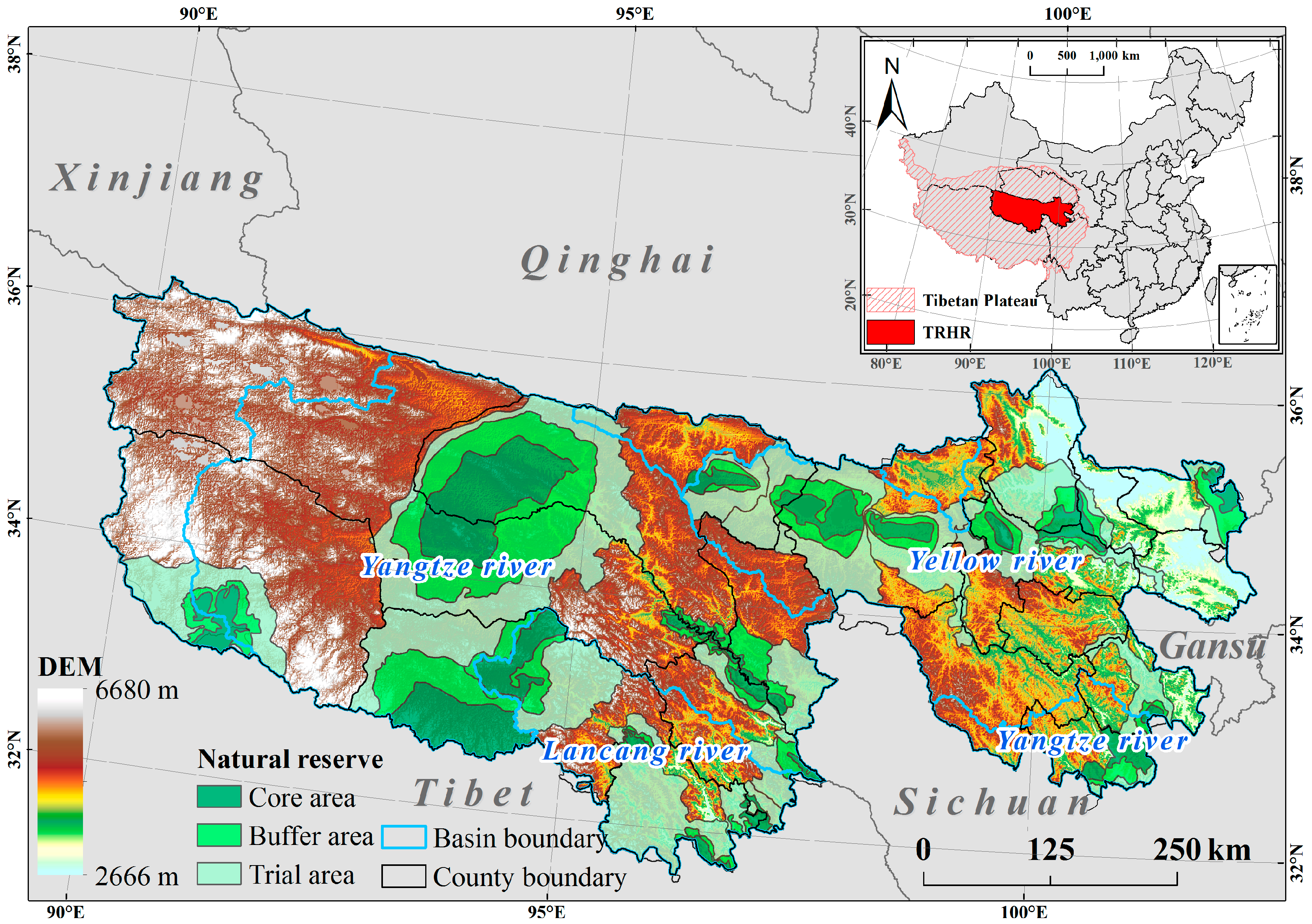
Between the 1980s and 2000, degradation of TRHR ecosystems took place consistently [44] and seriously interfered with the structure and function of regional local ecosystems and downstream areas. However, subsequent to 2005, an ecological reserve was gradually established within the TRHR, including core, buffer and trial areas (Figure 1). The purposes of this reserve included ecological protection and construction, infrastructure creation for the livelihoods and production of farmers and herders and supporting facilities for ecological protection. The area of the reserve incorporated 70 towns and villages encompassing four prefectures, 16 counties and one city, including Yushu County, Guoluo, Huangnan and Hainan prefectures and the city of Geermu. The total area of the reserve is 152,300 km2.
2.2. TRHR Climate Change
Because the average altitude of the TRHR is greater than 4500 m, this area is characterized by a cold and dry climate with an annual mean temperature of −3.03 °C. Temperature varies spatially between −13.34 and 4.98 °C, decreasing along a gradient from east-to-west, while annual precipitation is 428 mm, varying spatially between 144.16 and 728.51 mm and decreasing along a gradient from southeast-to-northwest. Between 2000 and 2012, the climatic conditions of the TRHR were characterized by a trend of warming and wetting, as revealed by time series data. Over the course of our study period, both precipitation and temperature increased annually by averages of 11.32 mm year−1 (p < 0.1) and 0.059 °C year−1 (p < 0.1), respectively (Figure 2). Data show that overall slope of annual mean temperature diminished from the southwest to the northeast, while in different basins and counties, the Lancang River basin, including Nangqian, Yushu, Zaduo and Zhiduo counties, experienced the largest annual temperature increase within the TRHR, followed by the Yangtze and Yellow river basins. The spatial distribution of wetting trends is characterized by a decrease from east-to-west, while the linear trend line slope of annual precipitation is 12.38 mm year−1 in the Yellow River basin, including Zeku, Henan and Chengduo counties, 10.23 mm year−1 in the Yangtze River basin and 8.72 mm year−1 in the Lancang River basin.
2.3. TRHR LULC between 2000 and 2012
Distributional data show that grasslands are intermittently distributed across the various counties of the TRHR, encompassing more than 65% of LULC types in the region (Figure 3a). The second most common LULC is unused land, encompassing more than 23% of total area and distributed in high-altitude zones in the middle and west of the region. Forested land is mainly distributed in the east and south of the TRHR, delineated by lakes and rivers, while construction and cultivated land occupy no more than 0.3% of total area and are distributed in various eastern counties.
Data show that areas of grassland and unused land within the TRHR shrank by 7664 km2 and 146 km2, respectively, between 2000 and 2012, while areas of water, cultivated, forested and construction land increased (Figure 3b). Specifically, the area of rivers and lakes increased by 5394 km2 compared with 2000 with the largest increase reaching 32.44%, while the areas of cultivated land and forested land increased by 7.48% and 16.80%, respectively. Over the same time period, the area of construction land shrank slightly, by around 0.18% compared with 2000.
Our results show that the total conversion area within the TRHR was 13.72 × 10⁴ km2 between 2000 and 2012, encompassing 38.85% of land area. Specifically, grassland, unused land and water were converted in the highest amounts (Figure 4), while the scale between 2000 and 2012 implies that 2.98% of total land area was converted. Based on outputs from geographic information systems (GIS) mapping and spatial analyses, it is clear that of the land converted out of grassland, a considerable proportion converted to unused land occurs in high-altitude areas in the west and south of the TRHR. Data also show that over the same period, about 5.90 × 10⁴ km2 of land were converted from other LULC types into grassland. Amongst different LULC types, 75.17% of newly-converted grassland was derived from unused land, especially in high-altitude districts and counties in northern areas. At the same time, 15.40% of newly-converted grassland was derived from forested land, mainly in districts and counties in the east of the TRHR. Unused land was mostly converted to grassland and water in 87.01% and 11.74% of converted areas, respectively; grassland newly-converted from unused land mostly occurred in the middle and northern regions of the TRHR, while newly-converted water from unused land is prevalent in high-altitude northwestern areas. The conversion of cultivated, forested and construction land is less common across the region, found mainly in various eastern counties of the TRHR.
3. Materials and Methods
In order to quantify the relationships between different ecosystem services within the TRHR, we initially utilized the Integrated Valuation of Ecosystem Services and Tradeoffs (InVEST) model to assess provisions. This model comprises a suite of GIS functions to evaluate the provision of ecosystem services. Specifically, the InVEST model is based on a series of production functions that defines how changes in the structure and function of an ecosystem are likely to affect the flow of ecosystem services across a landscape. We initially described the InVEST modules to be included in this analysis as water yield, soil conservation and nutrient export, before describing the data used to assess ecosystem services. Secondly, we developed a DMC method to analyze the relationships between different ecosystem services.
3.1. Ecosystem Service Assessment
3.1.1. Water Yield Module
In the context of the InVEST model, water yield is a basic rainfall-runoff module that incorporates local environmental conditions and LULC data as inputs and calculates net water balance at the watershed scale [45]. This module does not differentiate between surface, subsurface and baseflow, but assumes that all water yield from a given pixel reaches the point of interest via one of these alternative pathways. Thus, the model calculates the amount of water yield as the difference between precipitation and actual evapotranspiration (Equation (1)), as follows:
In this expression, Yxj denotes the water yield (mm) for LULC type j in a given grid cell, x, while Px refers to annual precipitation (mm) of this cell and AETxj is the actual annual evapotranspiration of LULC type j in the cell.
We adopted the output of this module, i.e., water yield (Yxj), to assess the water provision service. The inputs of this module include precipitation, potential evapotranspiration, the depth to root-restricting layer, plant available water fraction, LULC, watershed and biophysical table (the details are shown in Appendix A.1).
3.1.2. Sediment Delivery Ratio Module
The sediment delivery ratio (SDR) module is designed to map the overland sediment generation and its delivery to the stream [45]. This module calculates soil loss from a land unit using the universal soil loss equation (USLE) [46], with input data including topography, climate, vegetation and management practices. The InVEST model then applies an iterative analysis to estimate, for all pixels, the volume of soil eroded and trapped by downstream vegetation and erosion control practices given their capture and retention ability.
We therefore calculated the soil conservation services of vegetation and erosion control practices between 2000 and 2012; the first of these (soil conservation) was calculated as soil loss in the absence of vegetation cover including soil erosion control minus the soil loss for current LULC incorporating erosion control. The USLE model is the most widely-applied approach for soil erosion modeling and assessment and was applied to quantify and map annual soil loss in the two situations discussed in this paper. Soil conservation calculated using the USLE model is expressed as follows:
In this expression, ΔA denotes the amount of soil conservation (t ha−1 year−1), while A0 is potential soil erosion without vegetation cover (t ha−1 year−1) and Av is soil erosion given current land cover and management conditions (t ha−1 year−1). Thus, R, K, L and S denote rainfall erosivity (MJ mm ha−1 h−1 year−1), soil erodibility (t ha h ha−1 MJ−1 mm−1), slope length and slope angle factors, respectively, while C and P are the cover-management and support practice factors, respectively. Finally, L, S, C and P are all dimensionless factors (calculation details are given in Appendix A.2).
3.1.3. Nutrient Delivery Ratio Module
The nutrient delivery ratio (NDR) module is used for assessing the service of nutrient retention by natural vegetation [45]. An important proxy for pollution, the proportion of nutrients retained on each pixel is considered an important water quality indicator. This model generates a series of quantitative values for sediment exported from each pixel using two delivery ratios (one for nutrients transported by surface flow and the other for subsurface flow), as well as the product of this load, as follows:
In this expression, x denotes the quantitative value of nutrients exported from each pixel i, while loadsurf,i and loadsubs,i refer to the amounts of runoff nutrients transported by surface flow and groundwater, respectively. Thus, the nutrient load on each pixel is a function of upslope area and the downslope flow path (see the InVEST documentation for further information [45]). Similarly, NDRsurf,i and NDRsubs,i are the two delivery ratios; conceptually, the former represents the ability of a downstream pixel to transport nutrients through the surface flow without retention and incorporates a topographic index, while the latter denotes simple exponential decay with distance within the stream using a defined maximum value for subsurface nutrient retention. Thus, the nutrient total at the outlet of each watershed will be the sum of the contributions from all pixels within that watershed, as follows:
We adopted the output of this module (x) to assess the water purification. Input data in this case include a digital elevation model (DEM), LULC, proxies for nutrient runoff, the watershed, the biophysical table, subsurface retention efficiency and critical distance, as well as the accumulative value of threshold flow (details are given in Appendix A.3).
3.1.4. Data
We utilized LULC data for the TRHR obtained in 2000 as part of a remote sensing (RS) project to monitor the status of Chinese land use at a 1:100,000 scale. This project was initiated by the Chinese Academy of Science and resulted in a primary dataset of Landsat TM/ETM RS images alongside data that was subsequently generated using the human-computer interactive interpretation method. Thus, for consistency, we also employed 2012 land use data that were generated using this method of interpretation from HJ-1 (Huan Jing-1: Environmental Protection & Disaster Monitoring Constellation) images (i.e., a mini-satellite constellation that is used for environmental and disaster monitoring) that cover the entire TRHR. These LULC type data were classified into 25 categories, which were themselves subsequently grouped into six classes, encompassing cultivated land, forested land, grassland, rivers/lakes, construction land and unused land. The average interpretation accuracy of this LULC type classification was 97.5% for 2000 and 85.2% for 2012.
We obtained NPP data for the TRHR for 2000 and 2012 from [38]; these data were generated using the global production efficiency model, incorporating localized parameters extracted from large plot data obtained by cyclic sampling [47].
We obtained climate data for the period between 2000 and 2012 (including daily mean temperature and precipitation) from the China Meteorological Administration. These data were then used to calculate annual precipitation for the water yield model, rainfall erosivity for the soil conservation model and for analysis of climate variability. Climate data from different meteorological station records were interpolated onto raster-formatted surfaces using thin plate smoothing spline methods in the software ANUSPLIN 42 [48], while raster-formatted soil data, including the proportion of sand, silt, clay and the soil depth reference, all used to measure plant available water content (PAWC) in the water yield model and K in the soil conservation model, were extracted from the Harmonized World Soil Database [49]. A 30-m resolution DEM was then used to calculate slope length and slope angle to input into our soil conservation model.
3.2. DMC
The DMC method is often applied to verify the consistency of hydro-meteorological data. This approach compares data from a single station with a pattern generated using data from several other stations across a given area. We utilize the DMC method in this study in order to elucidate the relationships between different ecosystem services. However, as the elements we incorporated into our comparative analysis require high degrees of correlation, we performed an appropriate test for each pair of ecosystem services before constructing a graph.
In the case of two highly correlated variables, E1 and E2, which represent one pair of ecosystem services, the main procedure used to generate a DMC includes the initial calculation of ratios for each pair of functions based on raster map layers (E1/E2). This ensures that E2 decreases as values on the x-axis increase. Ratio grid cells on each map layer are then arranged based on their ascending values, and a scatter plot is generated by accumulating these values, which leads to a DMC for each pair of ecosystem services as in Equation (5), as follows:
In this expression, k denotes each ecosystem service observation, while the series y1, …, yk, denotes observations for E1, and the series x1, …, xk includes observations for E2.
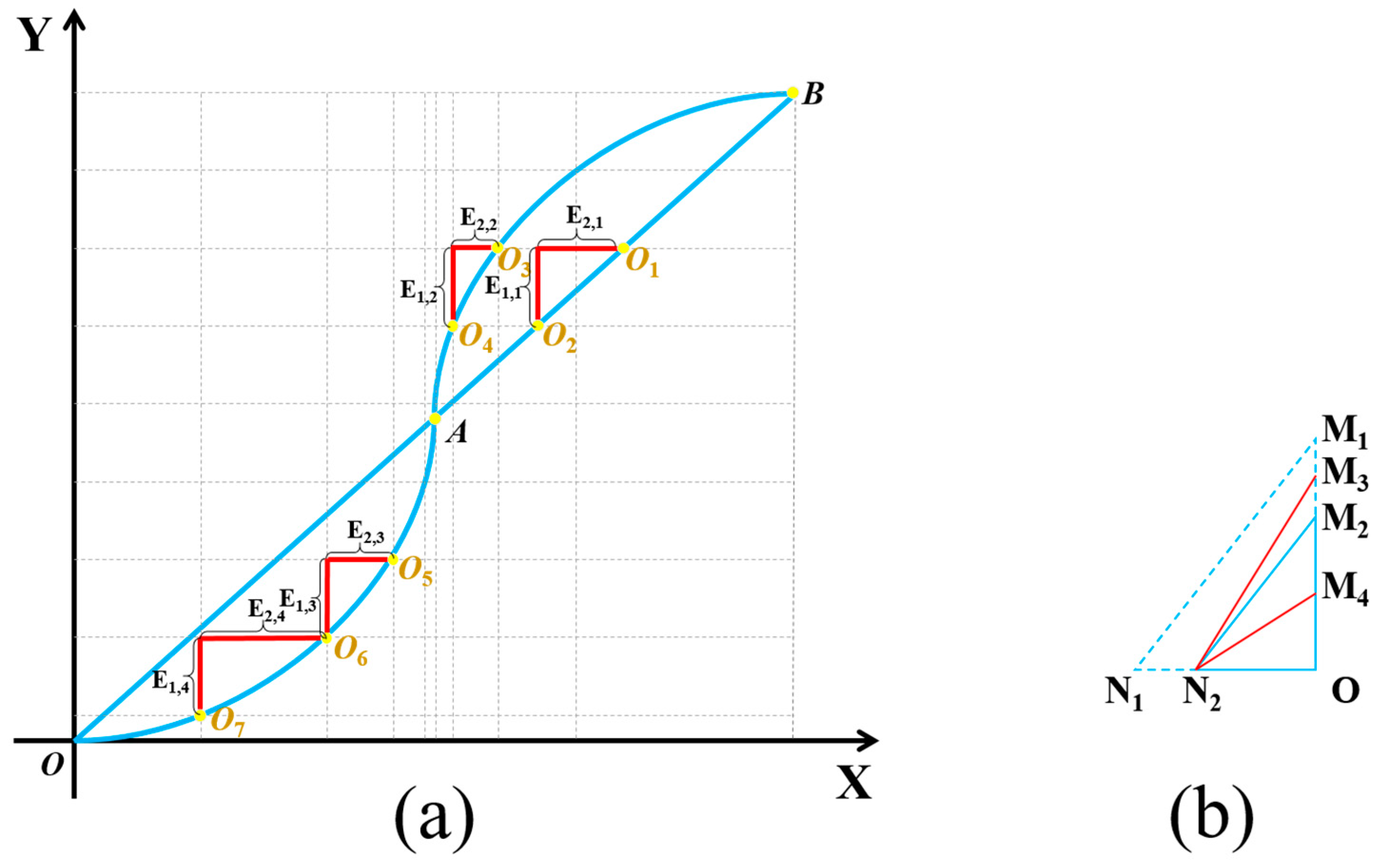
A graph drawn using this method can assume one of three different shapes, including a straight line (OA), a convex (AO3B) or concave curve (OO6A) (Figure 5). In order to conveniently illustrate these differences, we selected seven points (O1, O2, …, O7) on the curves; thus, points O1 and O2 are a straight line, while O3 to O7 are on the curves (Figure 5). Thus, for any point on the curve (i.e., O1,i, O2,i), the coordinate difference to its preceding counterpart (i.e., O1,i−1, O2,i−1) is its ecosystem service value (E1,i, E2,i), as expressed by Equation (6), as follows:
In the straight line case (OA), E2,i increases in concert with E1,i, while the ratio of changes in E1 versus a related E2 will be fixed. This relationship is expressed by Equation (7), as follows:
In this expression, ∆E denotes the change in E while C is constant.
Compared to a straight line, however, the slope of a curve (such as AO3B) is not fixed. This is expressed by Equation (8), as follows:
Thus, if the point O lies on the convex curve (Figure 5b), then the slope of this curve will decrease with increasing x-axis values. This indicates that point E1 on the convex curve will decrease (OM4) more than if it falls on a straight line (OM2); similarly, if point O lies on the concave curve, then the slope in this case will also increase with increasing x-axis values. This indicates that point E1 on the concave curve has increased (M2M3) relative to its position on a straight line (OM2).
Applying the definitions of synergies and trade-offs in ecosystem services, both a straight-line and a convex curve imply the simultaneous enhancement of two services that can be defined as synergistic. In contrast, a concave curve indicates that when the slope of a DMC changes, the provision of one ecosystem service is increased as a consequence of a reduction in another; this can be defined as a trade-off. The length of a DMC, as measured by graph axes, therefore represents the total ecosystem service amount for each component, while curvature indicates the relative closeness of a trade-off or a synergistic relationship. In other words, the greater the curvature, the closer the trade-off or synergistic relationship between two ecosystem services.
In order to contrast trade-offs in ecosystem services between different LULC types and altitudes, we randomly selected 500 sample plots (k = 500) encompassing cultivated land, forested land and grassland from a range of altitudes (i.e., less than 3500 m, between 3500 and 4500 m, between 4500 and 5500 m and greater than 5500 m) for further analysis.
4. Results
4.1. The Temporal and Spatial Distribution of Ecosystem Services within the TRHR
4.1.1. NPP
Data show that in 2000, the average NPP of ecosystems in the TRHR was 262.35 gC/m2/year, encompassing an overall total of 60.61 × 10⁶ tC. Breaking this down between LULC types, the NPP of forested land was largest, averaging 375 gC/m2/year, followed by cultivated land and grassland with averages of 252.73 gC/m2/year and 204.56 gC/m2/year, respectively. In contrast, the NPP of the TRHR in 2012 was 406.84 gC/m2/year, a 64.44% increase compared with 2000. Data show that the NPP of every LULC type increased over this time period; cultivated land increased the most, however, up to 118.12%, immediately followed by forested land, up to 75.83%, while NPP values for grassland changed the least, just 49.07%.
Because it is influenced by topography, rainfall, hours of daylight and vegetation type, the NPP of the TRHR exhibits strong spatial heterogeneity, decreasing gradually along a southeast-northwest transect (Figure 6a). The NPP of the Lancang River basin averages 332.76 gC/m2/year because temperature conditions are favorable and the rate of precipitation is relatively high; this region is followed by the Yellow and Yangtze river basins where the values are 232.46 gC/m2/year and 150.80 gC/m2/year, respectively. Data show that between 2000 and 2012, the NPP of the eastern Yellow River basin changed the most, 70.12%, while values for the Lancang River basin changed the least, just 30.28% (Figure 6b).
4.1.2. Water Yield
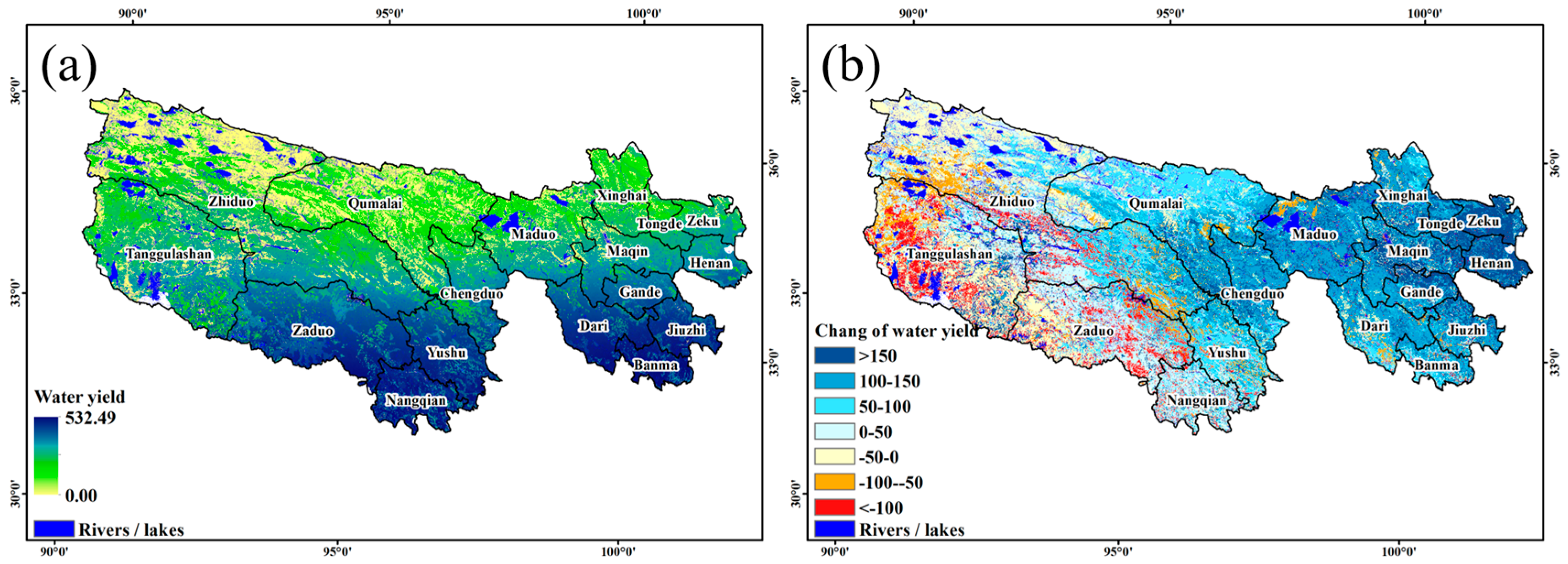
Our data show that the average water yield of the TRHR in 2000 was 147.41 mm, equivalent to a total amount of 5.05 × 10¹⁰ m3. However, compared to the “Qinghai Water Resources Bulletin” that was published in 2000 [50], our model calculation result is 0.20 × 10¹⁰ m3 higher than the total amount of surface water produced in the TRHR, a calculation error of 4.12%. In terms of LULC types, the average water yield from forested land was highest (average: 216.86 mm), followed by construction land and grassland (averages of 186.25 and 180.05 mm, respectively). Results show that by 2012, average water yield in the TRHR was 196.55 mm, corresponding to a total of 7.01 × 10¹⁰ m3 with a model calculation error of 1.74% [51]. Thus, compared with the water yield in 2000, data suggest an increase of 38.81%. The largest changes in water yields were seen in unused land, increasing from 43.65–103.63 mm (up 137.41%), followed by construction land and forested land that saw increases of 50.13% and 45.19%, respectively.
In terms of geographical distribution, average water yields in Banma Country were highest (Figure 7a), up to 368.51 mm, followed by the yields for Nangqian, Jiuzhi and Dari counties, which were up to 343.52, 313.86 and 313.86 mm, respectively. In contrast, high-altitude areas such as Zhiduo County and the Tanggulashan region experienced the lowest average water yields, up to just 14.06 and 71.27 mm, respectively. Across the whole TRHR, the average water yield of the Lancang River basin was highest (average: 314.51 mm), followed by the Yellow and Yangtze river basins that averaged 146.43 and 135.81 mm, respectively. Results show that between 2000 and 2012, the water yield increase in the east of the Yellow River basin was most significant throughout the whole area (Figure 7b), involving Zeku, Henan and Tongde counties and average increases greater than 145 mm. At the same time, however, average water yields of high-altitude areas obviously decreased, for example those of Tanggulashan, Zhiduo and southern Zaduo counties.
4.1.3. Soil Conservation
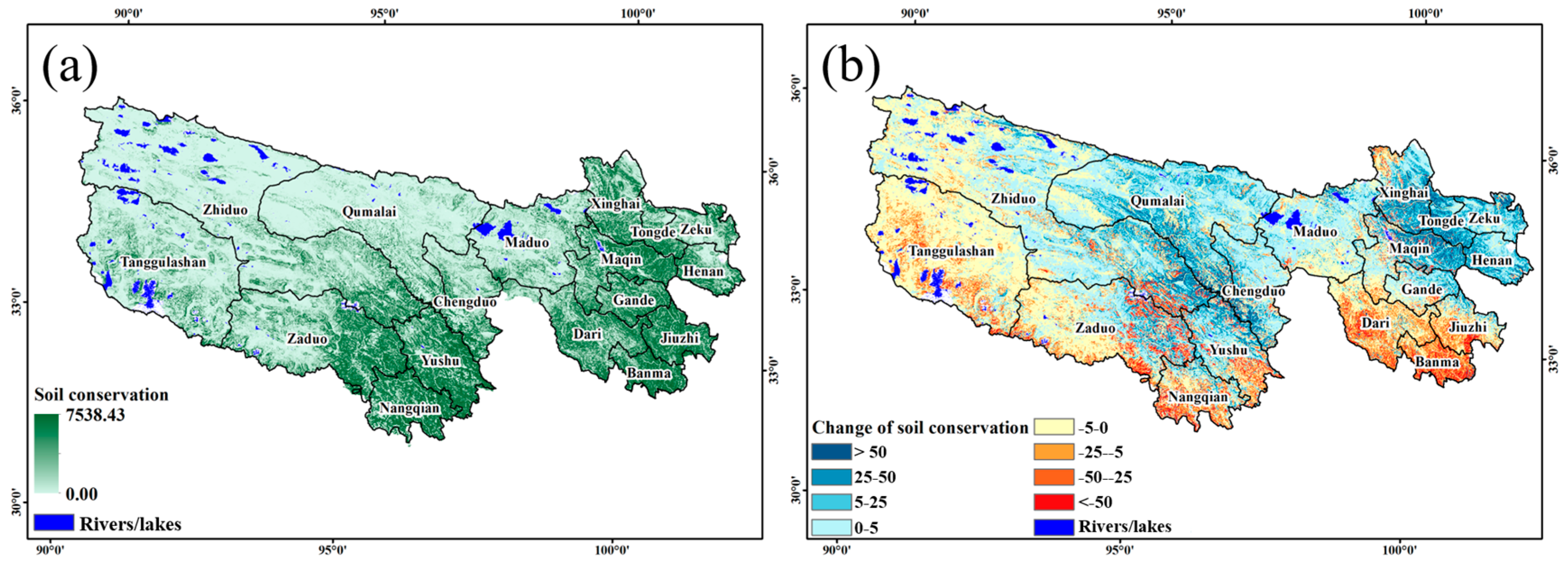
Data show that in 2000, average soil conservation within the TRHR was 3592 t km−2 (Figure 8). This equates to a total of 1.22 × 10⁹ t year−1, close to the result previously published by Wen [52] (i.e., total soil conservation amount: 1.06 × 10⁹ t year−1; average: 3662 t km−2). Amongst the areas involved, the Lancang River basin, including Nangqian, Yushu and Zaduo counties, and the southern Yangtze River basin, including Banma and Jiuzhi counties, experienced less slope erosion compared to other areas because they include dense and extensive forest and shrub coverage and thus a high proportion of conserved soil. In contrast, in 2012, the total amount of conserved soil across the whole region was 1.31 × 10⁹ t, an increase of 7.37%. Amongst the areas involved, Qumalai county experienced the greatest amplitude increases (average: 187.37%), while the Tanggulashan area and Dari, Banma, Zaduo and Jiuzhi counties saw their conserved soil proportions decrease (average: −21.81%).
4.1.4. P Export
Data show that in 2000, the average P export of the TRHR was 23.10 t km−2, equivalent to a total amount of 2.31 × 10⁷ t year−1. Across all LULC types, average P export from cultivated land was largest (average: 74.50 t km−2) followed by grassland and construction land, averaging 31.95 t km−2 and 26.99 t km−2, respectively. In contrast, P export from the forested land and unused land was relatively low, averaging 0.24 t km−2 and 0.28 t km−2, respectively. In 2012, the average P export of the TRHR was 13.50 t km−2, a decrease of 49.98% compared with 2000; within this, P export from cultivated land and grassland decreased by 4.93% and 40.48%, respectively, while that of the construction land, forested land and unused land increased by 1.88%, 12.50% and 142.86%, respectively.
Overall, our data show that P export from the TRHR decreases along a gradient from the southeast to the northwest (Figure 9a); within this, the average P export of the Lancang River basin was highest, up to 128.49 t km−2 and mainly including Yushu and Zaduo counties, followed by the Yangtze and Yellow river basins, up to 60.91 and 70.27 t km−2, respectively. Between 2000 and 2012, the average P export of every basin decreased (Figure 9b); within these data, the Lancang River basin exhibited the greatest decrease, 19.72%, while that of the Yellow River basin decreased the least, just 9.76%.
4.2. Synergies between Ecosystem Services
4.2.1. Correlations
We performed a correlation analysis of four ecosystem services within the TRHR, NPP, water yield, soil conservation and P export. Results reveal a positive relationship amongst these ecosystem services (Table 1); the correlation between water yield and NPP was highest, up to 0.761 for 2012 and 0.699 for 2000, followed by correlations between the amount of soil conservation and water yield. Lowest values are seen between the amount of P export and soil conservation. Data show that between 2000 and 2012, the coefficient of correlation between water yield and NPP increased, while those for other ecosystem services decreased.
4.2.2. Synergies
Assuming the accuracy of our DMC analysis, we selected four pairs of ecosystem services that exhibit average correlation coefficients greater than 0.3, and eliminated those between P export, NPP and soil conservation amount. In addition, to further analyze differences in synergy effects, we also established DMCs for different LULCs (i.e., cultivated land, forested land and grassland) and ranges of altitude (i.e., less than 3500 m, between 3500 and 4500 m, between 4500 and 5500 m and greater than 5500 m).
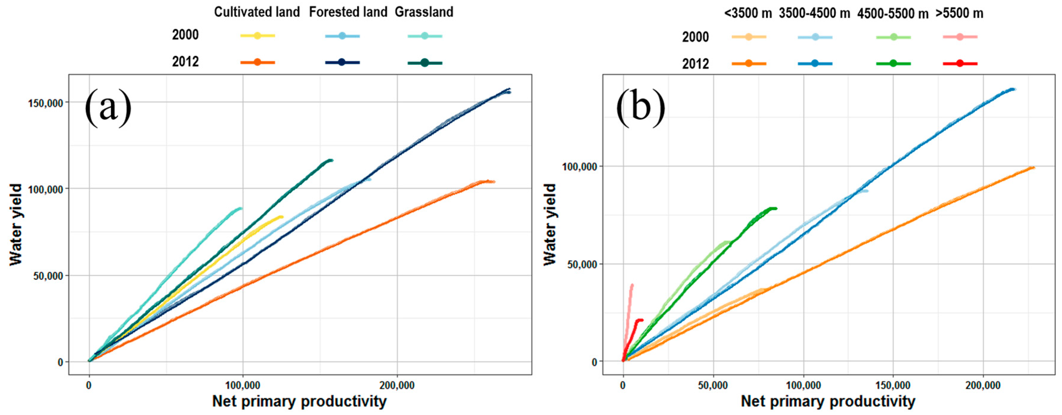
Results show that DMCs of NPP versus water yield for the TRHR conform to a linear relationship, indicating the presence of a fixed synergistic effect between the two services (Figure 8). Compared with data for 2000, the DMC of NPP and water yield for 2012 is extended, indicating an increased amount of accumulated NPP and water yield. This paired increasing trend in water yield and NPP for each LULC in 2012 shows that forested land and grassland are almost equivalent to one another and that both have larger values than cultivated land (Figure 10a). In addition, the DMC slope of these data increases in concert with altitude (Figure 10b), indicating that an improvement in NPP in high-altitude areas is favorable for enhancing water yields. Between 2000 and 2012, the total water yield amount and NPP both increased with altitude up to 5500 m, while a negative correlation was also present as amplitude and altitude increased. The slope rates of lines for all LULC types and ranges of altitude also decreased slightly compared with 2000, indicating a decreasing trend in water yield changes caused by unit changes in NPP.
The DMC graphs generated in this study to illustrate the amount of soil conservation versus NPP are characterized by some convex curve shapes, indicating the presence of a significant synergistic effect between this pair of services. Amongst different LULC types, the services provided by forested land were the highest (Figure 11a), followed successively by grassland and cultivated land. Thus, from the perspective of synergistic effects, as NPP decreased, the concomitant trend in reduction of the amount of soil conservation for each LULC was (from highest to lowest) forested land, grassland and cultivated land. Similarly, synergy between NPP and the amount of soil conservation is also positively correlated with altitude (Figure 11b). Results show that between 2000 and 2012, synergy between NPP and soil conservation for cultivated land decreased, while that for forested land and grassland remained broadly consistent. The change in synergies between NPP and soil conservation was, however, inconsistent for different altitude ranges; below 4500 m, synergy between the two services increased, but decreased at ranges above 4500 m.
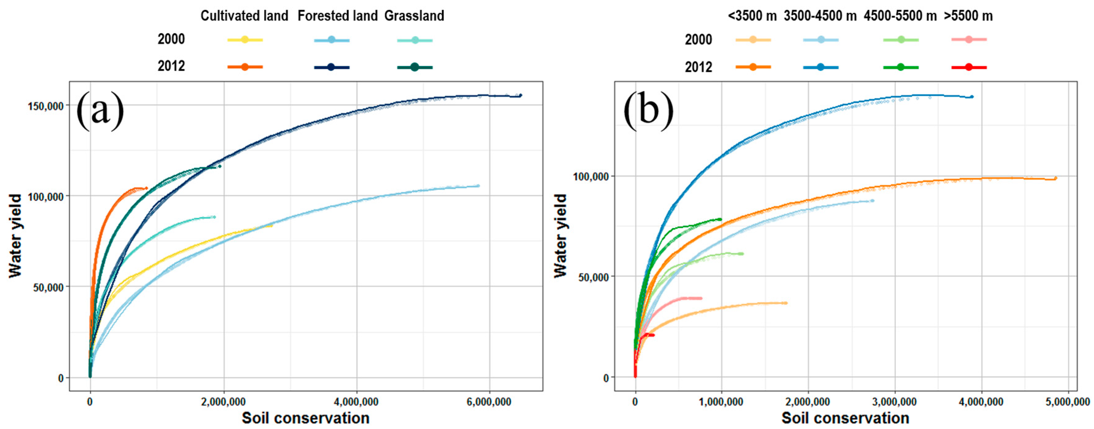
The DMC graphs generated in this study to illustrate the amount of soil conservation versus water yield for different LULCs corroborate the fact that the highest volume of services is provided by forested land, followed by grassland and cultivated land. In terms of synergistic effects, water yield amounts decrease in concert with soil conservation amounts with cultivated land greater than grassland, which is greater than forested land (Figure 12a). Across the different altitude ranges considered in this study, results reveal no positive correlation with either soil conservation or water yield (Figure 12b). However, when the amount of soil conservation is relatively large, its synergistic association with water yield remains consistent across all of the altitudes considered in this study. Results also show that when the soil conservation amount is reduced to a lower level, diverse synergies between the two services are seen at different altitudes. Between 2000 and 2012, an increasing trend between LULC types and latitudes is seen in the synergy between soil conservation and water yields; indeed, the trend towards an increase in the accumulated amount of water yield is greater than that for soil conservation. At altitudes below 4500 m, the accumulated provision of services tends to increase, while a concomitant reduction is seen above 4500 m.
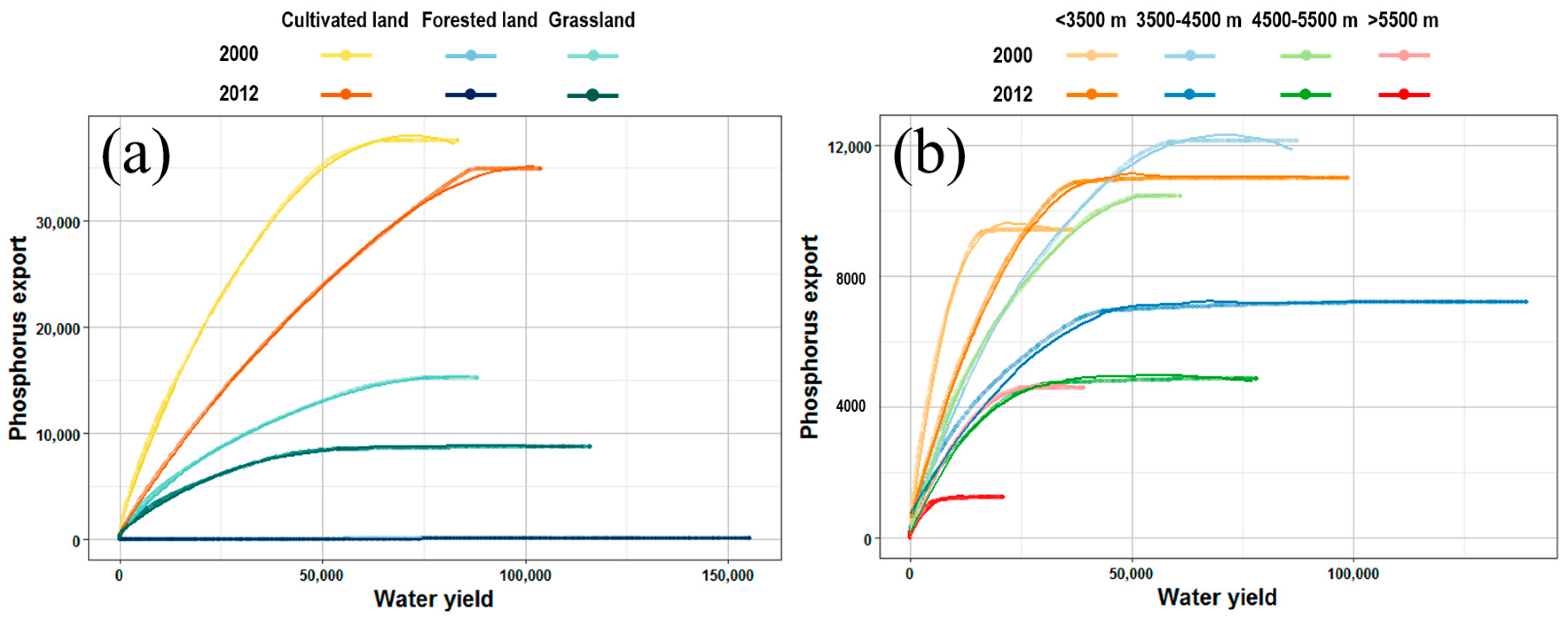
As the amount of P exported is very small when the water yields falls below a certain level, the DMCs expressing this relationship exhibit some convex curves of relatively low curvature and lines parallel to the x-axis. These shapes indicate significant synergy between this pair of services. Indeed, amongst the different LULC considered in this study, change in P export caused by a unit change in water yield on cultivated land was the highest (Figure 13a), followed by grassland and forested land. However, as the amount of P exported from forested land is very small, the DMC in this case plotted on the x-axis, while in terms of synergistic effects, compared with other ecosystem services pairs, the relationship between the amount of P export and water yield remains relatively fixed across the range of the latter. Results show that DMC slopes are positively correlated with altitude, however, which indicates that changes in the amount of P export caused by a unit change in water yield reduces along the gradient from high-to-low altitude (Figure 13b). Between 2000 and 2012, the synergy between the amount of exported P and water yield for all LULC types conformed to a decreasing trend.
5. Discussion
5.1. Key Factors Driving Changes in Ecosystem Services
It is well known that changes in ecosystem services are driven by both direct and indirect factors [53,54]. Although climate change is clearly the single most important direct factor, land conversions due to human exploitation and climate variability also influence both water use and plant growth [55,56]. Because the results of this study show that both land conversion and climatic factors significantly changed between 2000 and 2012 within the TRHR, we have evaluated changes in ecosystem services from both of these perspectives.
5.1.1. Climate Change
Changes in climate have consequences on the biophysical environment and include variation in potential evaporation, water supply and plant growth, as well as sediment and nutrient export. Data show that between 2000 and 2012, both precipitation and temperature increased annually by averages of 11.32 mm year−1 (p < 0.1) and 0.059 °C year−1 (p < 0.1), respectively, causing warming and wetting trends. The correlation analysis between annual changes in climate and ecosystem services presented in this paper shows that precipitation is an important climate variable, positively correlated with both NPP (R = 0.655, p < 0.01) and water yield (R = 0.478, p < 0.01). At the same time, temperature is negatively correlated with NPP (R = −0.186, p < 0.01). Our data show that increases in rainfall erosivity have significantly enhanced the amount of soil lost within the TRHR (R = 0.854, p < 0.01), an outcome with clear conservation implications. It is clear that vegetation coverage is a key factor in soil conservation [57,58]; our results show that increases in vegetation cover (measured by NPP) are positively correlated with controlling soil erosion (R = 0.217, p < 0.01). Similarly, the amount of exported P is a function of precipitation and hydrological conditions and is also positively correlated with rainfall erosivity (R = 0.161, p < 0.01); at the same time, the amount of exported P is rarely correlated with precipitation.
5.1.2. Land Conversion
Our results show that the highest number of ecosystem services, such as NPP, water yield and soil conservation, is provided by forested land, followed by grassland and cultivated land. In contrast, as agricultural land contains abundant nutrients, including P, which binds to sediments and occurs in freshwater, the volume of this element exported from this LULC is the highest within our dataset.
As the supply of ecosystem services varies with LULC types, both land conversion and management can influence this feedback in terms of both space and quantity [59]. Although the total areas of grassland and unused land (the two largest components of our dataset) have not varied a great deal between 2000 and 2012 (Figure 3b), conversion between them has been the most widespread within the TRHR, especially in high-altitude areas in the west and north (Figure 4). In Qumalai County, for example, the proportion of land converted from unused to grassland was the highest between 2000 and 2012, encompassing 47.78% of the total converted area. At the same time, however, total soil conservation also increased 187.37% over our study period; the amount of soil conservation per square kilometer on unconverted grasslands and on unused land increased by 10.08% and 8.86%, respectively, likely the result of changes in climate, while the proportion of land converted from unused to grassland increased 25.71%, a much higher proportion than for unconverted grassland. We can therefore conclude that land conversion is also a key factor underlying changes in ecosystem services.
5.2. Relationships between TRHR Ecosystem Services
The relationships between ecosystem services are often presented in different ways, including win-win, win-lose or win neutral scenarios. It is clear that the links between ecosystem services are complex and tight, and a range of studies has explicitly analyzed possible synergies and trade-offs. A number of previous studies has demonstrated the presence of a trade-off between water yield, NPP and soil conservation [20,60,61,62]; increases in NPP will decrease water yields and increase levels of soil conservation. The results presented here partially support these earlier conclusions, as we also identified synergies among the three ecosystem services, NPP, water yield and soil conservation. However, our results diverge from previous findings because we found synergy between water yields and NPP or soil conservation. This outcome was possible in this case because both climatic conditions and vegetation cover are relatively high within the TRHR. Taking into account the unique ecological environment, complicated landscape and topography of this region, it is clear that plant growth is strongly driven by precipitation and well-correlated with hydrological processes. Our results therefore demonstrate that both water yield and the amount of exported P exhibit synergies with one another depending on different LULC types and altitude ranges, especially in the case of low altitude agricultural land. Thus, since the amount of exported P is a proxy for water quality, this result also implies a trade-off between water yield and quality.
Numerous studies have also demonstrated highly non-linear relationships between different ecosystem services [63,64,65]. This is also the case in our results; we identify several non-linear synergies between our four pairs of ecosystem services, with the exception of water yield versus NPP. Thus, given the presence of both non-linear and synergistic relationships between ecosystem services, we demonstrate that increasing regional water yield enhances NPP and indirectly increases soil conservation; these relationships vary not only with altitude, but also depending on the amount of provision [19].
5.3. Uncertainties in Our Model-Based Assessment
We utilized the InVEST model in this study, incorporating water yield, sediment delivery ratio and nutrient delivery ratio modules, in order to assess the ecosystem services of the TRHR. However, as the resources that are required to perform model calibration and testing are scare, the results presented in this study cannot be easily calibrated against measurement data. We therefore calibrated our results by comparing them with datasets published in the literature. As a result, the most significant limitation of this study is that our model parameters are both uncertain and variable; biophysical tables were used, for example, as inputs for the nutrient delivery and sediment delivery ratio modules, while the overall InVEST model also has its own limitations [45]. Subsurface water, an important component of TRHR water resources, was not calculated by the water yield module as part of this analysis [19], while potential soil loss, included in the SDR module, included only water erosion as part of this calculation. This is a key shortcoming of this study as two other important kinds of soil erosion are also common in the TRHR, freeze-thaw and wind erosion [21].
5.4. Proposed Measures for the Sustainable Management of the TRHR
Assessing ecosystem services and evaluating their synergies are both critical and unavoidable parts of the natural resources decision-making process. The results of this study show that between 2000 and 2012, ecosystems within the TRHR were locally improved; the water yield of river basins increased by 30.85%; soil conservation ability increased by 33.33%, and NPP was enhanced by 64.44%. These results are indicative of significant ecological restoration achievements because of policy interference. A top-down governance structure is currently employed in the TRHR, and synergy between NPP, water yield, soil conservation and nutrient export has been shown to exist. The level of synergies, however, differs within this region depending on LULC types and natural conditions. Although climate change is the critical factor driving plant growth variations, land conversion and interactions between water and soils also alter the ecosystem service contribution of different LULC types. It will therefore be necessary to develop functional subdivisions of the TRHR in order to create mechanisms in support of protective actions, while ecosystem development is a necessary strategy to enhance environmental protection in the TRHR. At the moment, eco-management of the TRHR is controlled and implemented by the government; in the future, however, it will be critical to design and establish a synergistic conservation strategy for this unique ecosystem that is stakeholder motivated.
6. Conclusions
The results of this study show that between 2000 and 2012, degradation of grasslands was significant in high-altitude areas in the west of the TRHR (including the village of Tanggulashan, Zaduo and Zhiduo counties). At the same time, however, grassland increase in the middle and north of this region, encompassing Qumalai and Maduo counties, was less, while areas of transferred cultivated, forested and construction land were small and mainly located in eastern counties. It is also clear that the overall rate of LULC change in the TRHR was less than in other regions of the country.
As a result of the combined effects of climate change, human activities and ecological restoration projects, NPP, water yield and the amount of conserved soil within the TRHR increased between 2000 and 2012 by 64.44%, 38.81% and 7.37%, respectively, while the amount of exported P decreased by 49.98%. These results indicate an improvement in the ecosystem services of this region. Results also show that various ecosystem services decreased spatially along a gradient from southeast-to-northwest. The improvement amplitude of various ecosystem services in the Yellow River basin in the east was high, while less improvement was seen in the Yangtze and Lancang river basins. Local, obvious degradation was even seen in some places. Data show that, on average, the highest number of ecosystem services is provided by forested land, followed by grasslands and cultivated land. Throughout the TRHR, synergistic relationships are seen between NPP, water yield and the amount of soil conservation, indicating that increases in the former simultaneously increase the levels of the latter two services. Finally, the presence of a synergistic relationship between water yield and the amount of exported P indicates that increasing the former reduces the level of water purification.
Acknowledgments
This research was supported by the National Natural Science Foundation of China (Grant Nos. 41671177, 41501192 and 91325302), the National Basic Research Program of China (2015CB452702), and the National Key Research and Development Plan of China (2016YFA0602402).
Author Contributions
Wei Song designed the research, while Ze Han processed the data, developed the methodology, performed the research and wrote the manuscript. Wei Song reviewed the paper and supported the analyses, while Wei Song, Xiangzheng Deng and Xinliang Xu supervised the research and contributed with discussions and scientific advice.
Conflicts of Interest
The authors declare no conflict of interest.
Appendix A. Input Data of InVEST Models
Appendix A.1. Water Yield Module
According to the basic requirement of data input for this module, we calculated a number of key parameters. AETxj is a function of reference evapotranspiration, the depth of the root-restricting layer, plant available water content and LULC. It therefore follows that , the approximate value of the Budyko curve, can be calculated as follows:
In this expression, Rxj refers to Budyko’s aridity index of LULC type j in a given grid cell, x, and is equivalent to the ratio of potential evapotranspiration to precipitation. In contrast, ωx is dimensionless, denotes the water available to a plant and is used to estimate annual precipitation. Applying the definition of Zhang et al. [66], this non-physical parameter can also be used to describe soil attributes affected by natural climate and is calculated as follows:
In this expression, AWCx denotes the water available to a plant (mm) and will depend on both soil texture and depth, while Z refers to seasonal precipitation distribution and depth. Budyko’s aridity index is calculated as follows:
In this expression, ET0 is reference evapotranspiration, while kxj is the coefficient of evapotranspiration of LULC type j in a given grid cell, x, as determined by vegetation type.
We therefore defined average annual precipitation, ET0, soil depth, plant available water content (PAWC), LULC, root depth, elevation, biophysical table and the Z parameter as inputs to this water yield module. Of these, PAWC refers to the water fraction stored in the soil profile that is available for land use; this was calculated based on physical and chemical soil properties, following the method presented by Zhou [67], as follows:
This expression incorporates values for relative sand (sand%), silt (silt%), clay (clay%) and organic matter content (OM%).
We calculated the annual mean reference ET0 using the Food and Agriculture Organization of the United Nations (FAO) Penman–Monteith equation (Equation (A5), below) as listed in the user guide to the InVEST model [68], corrected using:
In this expression, LE is latent heat flux; D is the slope of the temperature saturated vapor pressure curve; Rn is net surface radiation; G is soil heat flux; r is air density; Cp is specific heat at constant pressure; Ta is air temperature; es (Ta − ea) denotes the vapor pressure difference at a reference height; γ is the psychrometric constant; ra is aerodynamic resistance; and rs is surface impedance.
Appendix A.2. Sediment Delivery Ratio Module
In this module, we also calculated a number of additional key parameters that are independent of the InVEST model. Of these, the soil erosive factor (K) was calculated by applying an erosion/productivity impact calculator model that is based on soil texture [69] using Equation (A6), as follows:
In this expression, SAN, SIL and CLA denote the sand (%), silt (%) and clay fractions (%), respectively, while C refers to soil organic carbon content (%), and SNI is equal to 1 − SAN/100. We also used a factor of 0.1317 to convert values from U.S. customary units to SI units.
Because the rainfall erosivity factor, R, equals the kinetic energy of rainfall, E, multiplied by the maximum rain intensity in a 30-min period I30 (cm h−1), use of this expression would require an unreasonably high frequency of rainfall events (i.e., one event every 30 min). We therefore customized the R factor calculation used in this study to a local context using half-month precipitation erosivity [70], a module that is already embedded in the Chinese soil loss equation [71], as follows:
In this expression, Rhj denotes half-month rainfall erosivity (MJ mm h m−2 h−1 year−1) while Pdi denotes effective rainfall for a given day, i, in one half-month period. Thus, Pdi is equal to actual rainfall if this value is larger than a threshold value of 12 mm, the standard for erosive rainfall in China. In all other cases, Pdi is equal to zero, while the term m refers to the number of days in the half-month period. The terms α and β are undetermined parameters, while Pd12 denotes the average daily rainfall more than 12 mm, and Py10 refers to the annual average rainfall for days when this level is exceeded.
We obtained values for the conservation practices (P) and cover type and management (C) factors from the USLE (handbook [46] and related studies [72] carried out in the TRHR (Table A1).

Table A1.
Biophysical values for factors C and P.
| LULC Type | C | P |
|---|---|---|
| Cultivated land | 0.300 | 1.000 |
| Forested land | 0.003 | 1.000 |
| Grassland | 0.020 | 1.000 |
| Rivers/lakes | 0.000 | 1.000 |
| Construction land | 0.000 | 1.000 |
| Unused land | 1.000 | 1.000 |
Appendix A.3. Nutrient Delivery Ratio Module
Input data in this module include a digital elevation model (DEM), LULC, proxies for nutrient runoff, the watershed, the biophysical table, subsurface retention efficiency and critical distance, as well as the accumulative value of threshold flow. Functioning as a quick flow index, the nutrient runoff proxy represents spatial variability in runoff potential in the form of a raster of normalized annual precipitation. Similarly, the biophysical table contains an LULC type code, as well as a corresponding descriptive name, the nutrient loading associated with each LULC type and maximum retention efficiency, the distance after which it is assumed that a patch of a particular LULC type retains a nutrient at its maximum capacity and the proportion of dissolved nutrients divided by the total amount of nutrients. These biophysical table parameters were also extracted from the InVEST user guide [45]; both the subsurface retention efficiency and critical distance were set to 150, the model default, while the threshold flow accumulation value, calibrated by comparing the river map with the stream map output by the model, was set to encompass an area of 600 pixels.
References
- Song, W.; Liu, M.L. Farmland conversion decreases regional and national land quality in China. Land Degrad. Dev. 2017, 28, 459–471. [Google Scholar] [CrossRef]
- Yu, G.; Chen, Z.; Zhang, L.; Peng, C.; Chen, J.; Piao, S.; Zhang, Y.; Niu, S.; Wang, Q.; Luo, Y.; et al. Recognizing the scientific mission of flux tower observation networks—Laying a solid scientific data foundation for solving ecological issues related to global change. J. Resour. Ecol. 2017, 8, 115–120. [Google Scholar]
- Ellis, E.C.; Klein Goldewijk, K.; Siebert, S.; Lightman, D.; Ramankutty, N. Anthropogenic transformation of the biomes, 1700 to 2000. Glob. Ecol. Biogeogr. 2010, 19, 589–606. [Google Scholar] [CrossRef]
- Alessa, L.; Chapin, F.S. Anthropogenic biomes: A key contribution to earth-system science. Trends Ecol. Evol. 2008, 23, 529–531. [Google Scholar] [CrossRef] [PubMed]
- Ellis, E.C.; Ramankutty, N. Putting people in the map: Anthropogenic biomes of the world. Front. Ecol. Environ. 2008, 6, 439–447. [Google Scholar] [CrossRef]
- Song, W.; Deng, X.Z. Effects of urbanization-induced cultivated land loss on ecosystem services in the North China Plain. Energies 2015, 8, 5678–5693. [Google Scholar] [CrossRef]
- Song, W.; Pijanowski, B.C.; Tayyebi, A. Urban expansion and its consumption of high-quality farmland in Beijing, China. Ecol. Indic. 2015, 54, 60–70. [Google Scholar] [CrossRef]
- Xiao, Y.; An, K.; Xie, G.; Lu, C. Evaluation of ecosystem services provided by 10 typical rice paddies in China. J. Resour. Ecol. 2011, 2, 328–337. [Google Scholar]
- Daily, G. Nature’s Services: Societal Dependence on Natural Ecosystems; Island Press: Washington, DC, USA, 1997. [Google Scholar]
- Bennett, E.M.; Peterson, G.D.; Gordon, L.J. Understanding relationships among multiple ecosystem services. Ecol. Lett. 2009, 12, 1394–1404. [Google Scholar] [CrossRef] [PubMed]
- Millennium Ecosystem Assessment. Ecosystems and Human Wellbeing: A Framework for Assessment; Island Press: Washington, DC, USA, 2003. [Google Scholar]
- Song, W.; Deng, X.; Yuan, Y.; Wang, Z.; Li, Z. Impacts of land-use change on valued ecosystem services on the rapidly urbanized North China Plain. Ecol. Model. 2015, 318, 245–253. [Google Scholar] [CrossRef]
- Lal, R. Soil carbon sequestration impacts on global climate change and food security. Science 2004, 304, 1623–1627. [Google Scholar] [CrossRef] [PubMed]
- Metzger, M.; Rounsevell, M.; Acosta-Michlik, L.; Leemans, R.; Schröter, D. The vulnerability of ecosystem services to land use change. Agric. Ecosyst. Environ. 2006, 114, 69–85. [Google Scholar] [CrossRef]
- Ke, X.; Zhan, J.; Ma, E.; Huang, J. Regional climate impacts of future urbanization in China. In Land Use Impacts on Climate; Springer: Berlin/Heidelberg, Germany, 2014; pp. 167–206. [Google Scholar]
- Schroter, D.; Cramer, W.; Leemans, R.; Prentice, I.C.; Araujo, M.B.; Arnell, N.W.; Bondeau, A.; Bugmann, H.; Carter, T.R.; Gracia, C.A.; et al. Ecosystem service supply and vulnerability to global change in Europe. Science 2005, 310, 1333–1337. [Google Scholar] [CrossRef] [PubMed]
- Cramer, W.; Bondeau, A.; Woodward, F.I.; Prentice, I.C.; Betts, R.A.; Brovkin, V.; Cox, P.M.; Fisher, V.; Foley, J.A.; Friend, A.D.; et al. Global response of terrestrial ecosystem structure and function to CO2 and climate change: Results from six dynamic global vegetation models. Glob. Chang. Biol. 2001, 7, 357–373. [Google Scholar] [CrossRef]
- Holling, C.S. The resilience of terrestrial ecosystems: Local surprise and global change. Sustain. Dev. Biosph. 1986, 14, 292–317. [Google Scholar]
- Liu, F.; Zhang, H.; Zhang, Y.; Zhou, Q.; Duo, H. A study on the resources using and environment policy in the Three River’s source nature reserve. J. Qinghai Norm. Univ. Nat. Sci. 2005, 2, 86–91. (In Chinese) [Google Scholar]
- Jiang, C.; Li, D.; Wang, D.; Zhang, L. Quantification and assessment of changes in ecosystem service in the Three-River headwaters region, China as a result of climate variability and land cover change. Ecol. Indic. 2016, 66, 199–211. [Google Scholar] [CrossRef]
- Lawler, J.J.; Lewis, D.J.; Nelson, E.; Plantinga, A.J.; Polasky, S.; Withey, J.C.; Helmers, D.P.; Martinuzzi, S.; Pennington, D.; Radeloff, V.C. Projected land-use change impacts on ecosystem services in the United States. Proc. Natl Acad. Sci. USA 2014, 111, 7492–7497. [Google Scholar] [CrossRef] [PubMed]
- Zhang, J.J.; Fu, M.C.; Zhang, Z.Y.; Tao, J.; Fu, W. A trade-off approach of optimal land allocation between socio-economic development and ecological stability. Ecol. Model. 2014, 272, 175–187. [Google Scholar] [CrossRef]
- Jia, X.Q.; Fu, B.J.; Feng, X.M.; Hou, G.H.; Liu, Y.; Wang, X.F. The trade-off and synergy between ecosystem services in the grain-for-green areas in Northern Shaanxi, China. Ecol. Indic. 2014, 43, 103–113. [Google Scholar] [CrossRef]
- Tallis, H.; Kareiva, P.; Marvier, M.; Chang, A. An ecosystem services framework to support both practical conservation and economic development. Proc. Natl Acad. Sci. USA 2008, 105, 9457–9464. [Google Scholar] [CrossRef] [PubMed]
- Xie, H.; Yao, G.; Liu, G. Spatial evaluation of the ecological importance based on gis for environmental management: A case study in Xingguo County of China. Ecol. Indic. 2015, 51, 3–12. [Google Scholar] [CrossRef]
- Emily, N.; Georginam, M.; Paulr, A.; Giles, A.; Simon, B.; Tom, C.; Robertm, E.; Johne, F.; Tobya, G.; James, G. Priority research areas for ecosystem services in a changing world. J. Appl. Ecol. 2009, 46, 1139–1144. [Google Scholar]
- Dobson, A.; Lodge, D.; Alder, J.; Cumming, G.S.; Keymer, J.; Mcglade, J.; Mooney, H.; Rusak, J.A.; Sala, O.; Wolters, V. Habitat loss, trophic collapse, and the decline of ecosystem services. Ecology 2006, 87, 1915–1924. [Google Scholar] [CrossRef]
- Carpenter, S.R.; Bennett, E.M.; Peterson, G.D. Scenarios for ecosystem services: An overview. Ecol. Soc. 2006, 11, 1599–1604. [Google Scholar] [CrossRef]
- Bryan, B.A. Incentives, land use, and ecosystem services: Synthesizing complex linkages. Environ. Sci. Policy 2013, 27, 124–134. [Google Scholar] [CrossRef]
- Coggan, A.; Whitten, S.M.; Bennett, J. Influences of transaction costs in environmental policy. Ecol. Econ. 2010, 69, 1777–1784. [Google Scholar] [CrossRef]
- Villamagna, A.M.; Angermeier, P.L.; Bennett, E.M. Capacity, pressure, demand, and flow: A conceptual framework for analyzing ecosystem service provision and delivery. Ecol. Complex. 2013, 15, 114–121. [Google Scholar] [CrossRef]
- Li, S.; Zhang, C.; Liu, J.; Zhu, W.; Ma, C.; Wang, J. The trade-offs and synergies of ecosystem services: Research progress, development trend, and themes of geography. Geogr. Res. 2013, 32, 1379–1390. [Google Scholar]
- Turner, K.G.; Odgaard, M.V.; Bocher, P.K.; Dalgaard, T.; Svenning, J.C. Bundling ecosystem services in Denmark: Trade-offs and synergies in a cultural landscape. Landsc. Urban Plan. 2014, 125, 89–104. [Google Scholar] [CrossRef]
- Deng, X.Z.; Li, Z.H.; Gibson, J. A review on trade-off analysis of ecosystem services for sustainable land-use management. J. Geogr. Sci. 2016, 26, 953–968. [Google Scholar] [CrossRef]
- Briner, S.; Huber, R.; Bebi, P.; Elkin, C.; Schmatz, D.; Grêt-Regamey, A. Trade-offs between ecosystem services in a mountain region. Ecol. Soc. 2013, 18, 35. [Google Scholar] [CrossRef]
- Jiang, C.; Li, D.; Gao, Y.; Liu, W.; Zhang, L. Impact of climate variability and anthropogenic activity on streamflow in the Three-Rivers Headwater region, Tibetan Plateau, China. Theor. Appl. Climatol. 2017, 129, 667–681. [Google Scholar] [CrossRef]
- Jiang, C.; Zhang, L. Effect of ecological restoration and climate change on ecosystems: A case study in the Three-Rivers Headwater region, China. Environ. Monit. Assess. 2016, 188, 382. [Google Scholar] [CrossRef] [PubMed]
- Xu, X.L.; Xiao, T.; Zhan, Z.M.; Tian, J.L.; Ge, J.S. Atlas of Remote Sensing for Ecosystems in the “Three Rivers Headwaters” Region of Qinghai Province; Star Map Press: Beijing, China, 2015. [Google Scholar]
- Jiang, C.; Zhang, L.B. Ecosystem change assessment in the Three-River Headwater region, China: Patterns, causes, and implications. Ecol. Eng. 2016, 93, 24–36. [Google Scholar] [CrossRef]
- Wang, Z.Q.; Zhang, Y.Z.; Yang, Y.; Zhou, W.; Gang, C.C.; Zhang, Y.; Li, J.L.; An, R.; Wang, K.; Odeh, I.; et al. Quantitative assess the driving forces on the grassland degradation in the Qinghai-Tibet Plateau, in China. Ecol. Inform. 2016, 33, 32–44. [Google Scholar] [CrossRef]
- Zhang, Y.; Zhang, C.; Wang, Z.; Chen, Y.; Gang, C.; An, R.; Li, J. Vegetation dynamics and its driving forces from climate change and human activities in the Three-River Source Region, China from 1982 to 2012. Sci. Total Environ. 2016, 563–564, 210–220. [Google Scholar] [CrossRef] [PubMed]
- Li, S.; Wang, Z.; Zhang, Y.; Wang, Y.; Liu, F. Comparison of socioeconomic factors between surrounding and non-surrounding areas of the Qinghai-Tibet railway before, and after, its construction. Sustainability 2016, 8, 776. [Google Scholar] [CrossRef]
- Li, X.; Brierley, G.; Shi, D.; Xie, Y.; Sun, H. Ecological protection and restoration in Sanjiangyuan national nature reserve, Qinghai Province, China. In Perspectives on Environmental Management and Technology in Asian River Basins; Springer: Berlin/Heidelberg, Germany, 2012; pp. 93–120. [Google Scholar]
- Fang, Y. Managing the Three-Rivers Headwater region, China: From ecological engineering to social engineering. Ambio 2013, 42, 566–576. [Google Scholar] [CrossRef] [PubMed]
- Sharp, R.; Tallis, H.; Ricketts, T.; Guerry, A.; Wood, S.; Chaplin-Kramer, R.; Nelson, E.; Ennaanay, D.; Wolny, S.; Olwero, N. InVEST 3.3.2 User’s Guide. In The Natural Capital Project, Stanford; Stanford University Press: Redwood, CA, USA, 2014. [Google Scholar]
- Renard, K.G. Predicting soil erosion by water: A guide to conservation planning with the revised universal soil loss equation (RUSLE). In Agricultural Handbook No. 703; U.S. Department of Agriculture, U.S. Government Printing Office: Washington, DC, USA, 1997; p. 404. [Google Scholar]
- Chen, Z.; Shao, Q.; Liu, J.; Wang, J. Analysis of net primary productivity of terrestrial vegetation on the Qinghai-Tibet Plateau, based on Modis remote sensing data. Sci. China Earth Sci. 2012, 55, 1306–1312. [Google Scholar] [CrossRef]
- Hutchinson, M.F.; Xu, T. Anusplin Version 4.2 User Guide; Centre for Resource and Environmental Studies, The Australian National University: Canberra, Australia, 2004; Available online: http://fennerschool.anu.edu.au/files/anusplin44.pdf (accessed on 3 August 2017).
- Nachtergaele, F.; van Velthuizen, H.; Verelst, L.; Batjes, N.; Dijkshoorn, K.; van Engelen, V.; Fischer, G.; Jones, A.; Montanarella, L.; Petri, M. Harmonized World Soil Database; Version 1.2; Wageningen: Rome, Italy, 2009. [Google Scholar]
- The Ministry of Water Resources of the People’s Republic of China. Qinghai Water Resources Bulletin; Qinghai Provincial Department of Water Resources: Qinghai, China, 2000; p. 31.
- The Ministry of Water Resources of the People’s Republic of China. Qinghai Water Resources Bulletin; Qinghai Provincial Department of Water Resources: Qinghai, China, 2012; p. 31.
- Wen, L. Assessment of Soil Conservation in Sanjiangyuan Based on the Invest Model; Capital Normal University: Beijing, China, 2012. [Google Scholar]
- Nelson, G.C.; Dobermann, A.; Nakicenovic, N.; O’Neill, B. Anthropogenic drivers of ecosystem change: An overview. Ecol. Soc. 2006, 11, 29. [Google Scholar] [CrossRef]
- Lead, C.; Nelson, G.C.; Bennett, E. Drivers of change in ecosystem condition and services. Ecosyst. Hum. Well-Being 2005, 2, 172–222. [Google Scholar]
- Oliver, T.H.; Morecroft, M.D. Interactions between climate change and land use change on biodiversity: Attribution problems, risks, and opportunities. Wiley Interdiscip. Rev. Clim. Chang. 2014, 5, 317–335. [Google Scholar] [CrossRef] [Green Version]
- Bellard, C.; Bertelsmeier, C.; Leadley, P.; Thuiller, W.; Courchamp, F. Impacts of climate change on the future of biodiversity. Ecol. Lett. 2012, 15, 365–377. [Google Scholar] [CrossRef] [PubMed]
- Zhang, Y.; Liu, B.; Zhang, Q.; Xie, Y. Effect of different vegetation types on soil erosion by water. Acta Bot. Sin. 2002, 45, 1204–1209. [Google Scholar]
- Laker, M. Advances in soil erosion, soil conservation, land suitability evaluation and land use planning research in South Africa, 1978–2003. S. Afr. J. Plant. Soil 2004, 21, 345–368. [Google Scholar] [CrossRef]
- Sharps, K.; Masante, D.; Thomas, A.; Jackson, B.; Redhead, J.; May, L.; Prosser, H.; Cosby, B.; Emmett, B.; Jones, L. Comparing strengths and weaknesses of three ecosystem services modelling tools in a diverse UK river catchment. Sci. Total Environ. 2017, 584, 118–130. [Google Scholar] [CrossRef] [PubMed]
- Zheng, Z.; Fu, B.; Hu, H.; Sun, G. A method to identify the variable ecosystem services relationship across time: A case study in the Yanhe Basin, China. Landsc. Ecol. 2014, 29, 1689–1696. [Google Scholar] [CrossRef]
- Tian, Y.; Wang, S.; Bai, X.; Luo, G.; Xu, Y. Trade-offs among ecosystem services in a typical karst watershed, SW China. Sci. Total Environ. 2016, 566, 1297–1308. [Google Scholar] [CrossRef] [PubMed]
- Zheng, Z.; Fu, B.; Feng, X. GIS-based analysis for hotspot identification of trade-off between ecosystem services: A case study in the Yanhe Basin, China. Chin. Geogr. Sci. 2016, 26, 466–477. [Google Scholar] [CrossRef]
- Howe, C.; Suich, H.; Vira, B.; Mace, G.M. Creating win-wins from trade-offs? Ecosystem services for human well-being: A meta-analysis of ecosystem service trade-offs and synergies in the real world. Glob. Environ. Chang. 2014, 28, 263–275. [Google Scholar] [CrossRef]
- Farber, S.C.; Costanza, R.; Wilson, M.A. Economic and ecological concepts for valuing ecosystem services. Ecol. Econ. 2002, 41, 375–392. [Google Scholar] [CrossRef]
- Van Jaarsveld, A.; Biggs, R.; Scholes, R.; Bohensky, E.; Reyers, B.; Lynam, T.; Musvoto, C.; Fabricius, C. Measuring conditions and trends in ecosystem services at multiple scales: The southern African millennium ecosystem assessment (SAFMA) experience. Philos. Trans. R. Soc. Lond. B Biol. Sci. 2005, 360, 425–441. [Google Scholar] [CrossRef] [PubMed]
- Zhang, L.; Hickel, K.; Dawes, W.; Chiew, F.H.; Western, A.; Briggs, P. A rational function approach for estimating mean annual evapotranspiration. Water Resour. Res. 2004, 40. [Google Scholar] [CrossRef]
- Zhou, W.; Liu, G.; Pan, J.; Feng, X. Distribution of available soil water capacity in China. J. Geogr. Sci. 2005, 15, 3–12. [Google Scholar] [CrossRef]
- Allen, R.G.; Pereira, L.S.; Raes, D.; Smith, M. Crop evapotranspiration-guidelines for computing crop water requirements-FAO irrigation and drainage paper 56. FAO Rome 1998, 300, D05109. [Google Scholar]
- Williams, J.; Arnold, J. A system of erosion—Sediment yield models. Soil Technol. 1997, 11, 43–55. [Google Scholar] [CrossRef]
- Zhang, W.; Fu, J. Rain erositivity estimation under different rainfall amount. Resour. Sci. 2002, 25, 35–41. [Google Scholar]
- Liu, B.; Zhang, K.; Xie, Y. An empirical soil loss equation. In Proceedings of the 12th International Soil Conservation Organization Conference, Beijing, China, 26–31 May 2002; p. 15. (In Chinese). [Google Scholar]
- Li, S.; Wang, Z.; Zhang, Y. Crop cover reconstruction and its effects on sediment retention in the tibetan plateau for 1900–2000. J. Geogr. Sci. 2017, 27, 786–800. [Google Scholar] [CrossRef]
Figure 1.
Map to show the geographic location of the Three-Rivers Headwaters region (TRHR). This natural reserve contains three regions encompassing core, buffer and trial areas; of these, the first is strictly managed with no grazing allowed and the implementation of measures to protect endangered species. Thus, all development and land use within the core zone are prohibited; this is a “no man zone”, and all former residents have been resettled elsewhere. Conservation is promoted in the buffer area alongside limited and rotational grazing, while the trial area is used for scientific investigations, eco-tourism and other green industries.

Figure 2.
Changes in annual precipitation (a) and annual mean temperature (b) between 2000 and 2012 (90% confidence levels).
Figure 2.
Changes in annual precipitation (a) and annual mean temperature (b) between 2000 and 2012 (90% confidence levels).
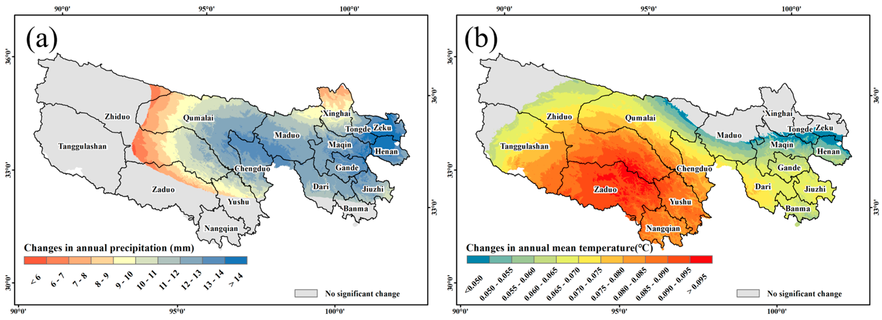
Figure 3.
The geographical distribution of LULC types within the TRHR in 2000 (a) and changes between 2000 and 2012 (b).
Figure 3.
The geographical distribution of LULC types within the TRHR in 2000 (a) and changes between 2000 and 2012 (b).
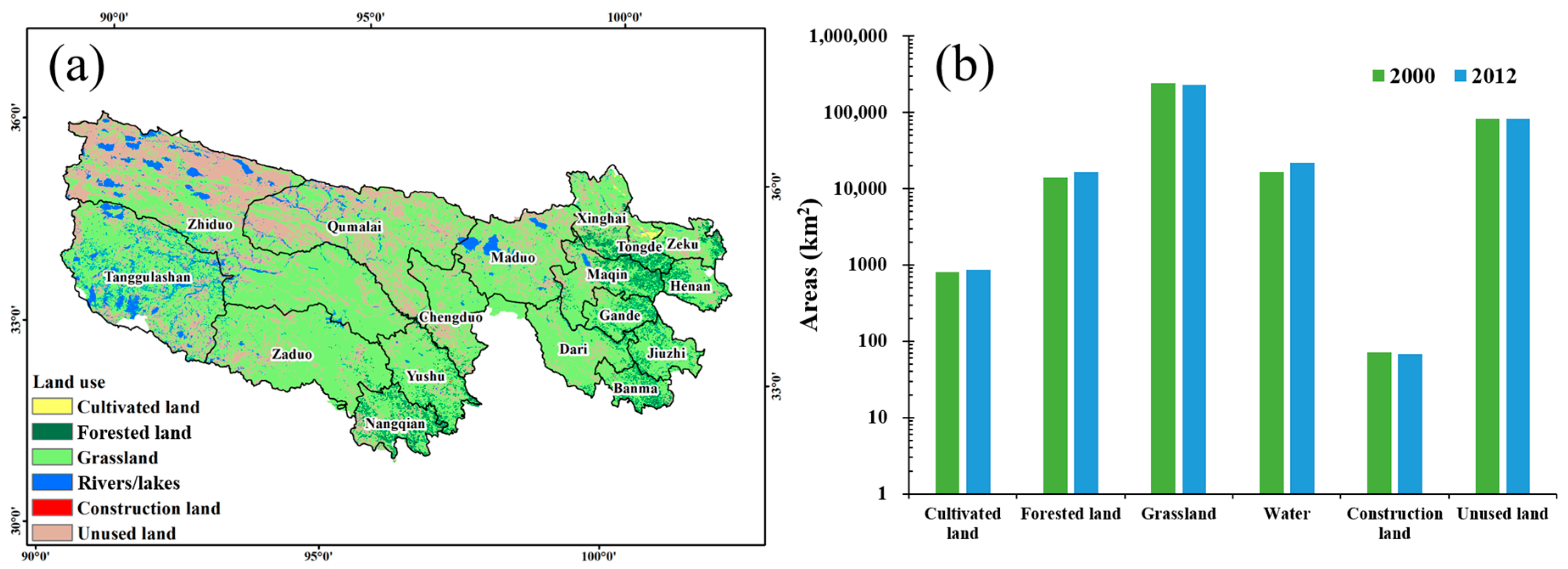
Figure 4.
Maps to show the geographical distribution of converted land within the TRHR in 2000 (a) and 2012 (b).
Figure 4.
Maps to show the geographical distribution of converted land within the TRHR in 2000 (a) and 2012 (b).
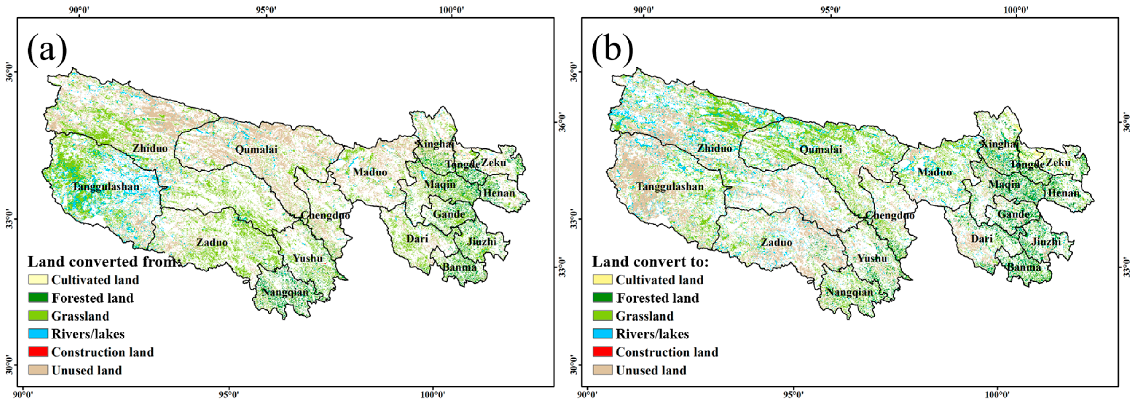
Figure 5.
Double mass curve (DMC) sketches (a) and comparisons between different slopes of DMC (b).

Figure 6.
Maps to show the spatial distribution of NPP in the TRHR in 2000 (a) and change up to 2012 (b) (unit: gC m−2).
Figure 6.
Maps to show the spatial distribution of NPP in the TRHR in 2000 (a) and change up to 2012 (b) (unit: gC m−2).
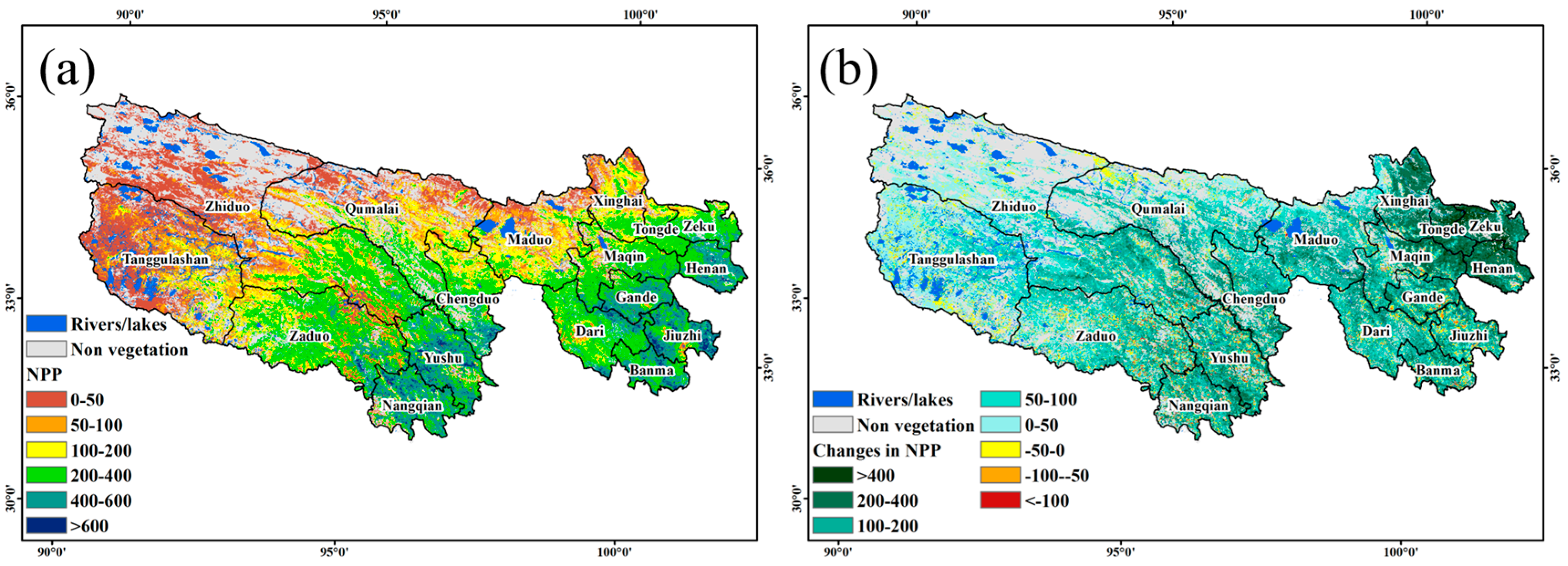
Figure 7.
Maps to show the spatial distribution of water yield in the TRHR in 2000 (a) and change up to 2012 (b).
Figure 7.
Maps to show the spatial distribution of water yield in the TRHR in 2000 (a) and change up to 2012 (b).

Figure 8.
Maps to show the spatial distribution of soil conservation amount in the TRHR in 2000 (a) and change up to 2012 (b).
Figure 8.
Maps to show the spatial distribution of soil conservation amount in the TRHR in 2000 (a) and change up to 2012 (b).

Figure 9.
Maps to show the spatial distribution of P export in the TRHR in 2000 (a) and change up to 2012 (b).
Figure 9.
Maps to show the spatial distribution of P export in the TRHR in 2000 (a) and change up to 2012 (b).
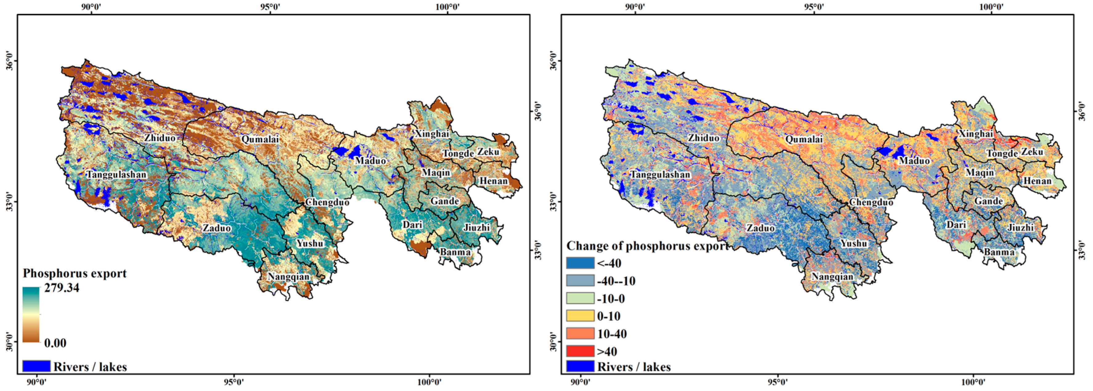
Figure 10.
DMC graphs of water yield versus NPP for the different types of land use (a) and different altitude ranges (b) in the TRHR.
Figure 10.
DMC graphs of water yield versus NPP for the different types of land use (a) and different altitude ranges (b) in the TRHR.

Figure 11.
DMC graphs of soil conservation amount versus NPP for the different types of land use (a) and different altitude ranges (b) in the TRHR.
Figure 11.
DMC graphs of soil conservation amount versus NPP for the different types of land use (a) and different altitude ranges (b) in the TRHR.
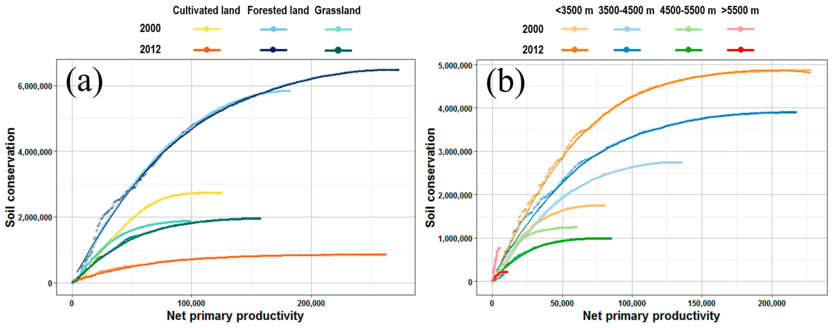
Figure 12.
DMC graphs of water yield versus soil conservation for the different types of land use (a) and different altitude ranges (b) in the TRHR.
Figure 12.
DMC graphs of water yield versus soil conservation for the different types of land use (a) and different altitude ranges (b) in the TRHR.

Figure 13.
DMC graphs of P exported versus water yield for the different types of land use (a) and different altitude ranges (b) in the TRHR.
Figure 13.
DMC graphs of P exported versus water yield for the different types of land use (a) and different altitude ranges (b) in the TRHR.

Table 1.
Correlation matrix between various ecosystem services of the TRHR.
| Year | Ecosystem Service | NPP | Water Yield | Soil Conservation | P Export |
|---|---|---|---|---|---|
| 2000 | NPP | 1 | |||
| Water yield | 0.699 *** | 1 | |||
| Soil conservation | 0.383 *** | 0.407 *** | 1 | ||
| P export | 0.309 *** | 0.500 *** | 0.224 *** | 1 | |
| 2012 | NPP | 1 | |||
| Water yield | 0.761 *** | 1 | |||
| Soil conservation | 0.338 *** | 0.294 *** | 1 | ||
| P export | 0.095 *** | 0.178 *** | 0.066 *** | 1 |
Note: *** Correlation is significant at the 0.01 level (two-tailed).
© 2017 by the authors. Licensee MDPI, Basel, Switzerland. This article is an open access article distributed under the terms and conditions of the Creative Commons Attribution (CC BY) license (http://creativecommons.org/licenses/by/4.0/).
Share and Cite
MDPI and ACS Style
Han, Z.; Song, W.; Deng, X.; Xu, X. Trade-Offs and Synergies in Ecosystem Service within the Three-Rivers Headwater Region, China. Water 2017, 9, 588. https://doi.org/10.3390/w9080588
AMA Style
Han Z, Song W, Deng X, Xu X. Trade-Offs and Synergies in Ecosystem Service within the Three-Rivers Headwater Region, China. Water. 2017; 9(8):588. https://doi.org/10.3390/w9080588
Chicago/Turabian StyleHan, Ze, Wei Song, Xiangzheng Deng, and Xinliang Xu. 2017. "Trade-Offs and Synergies in Ecosystem Service within the Three-Rivers Headwater Region, China" Water 9, no. 8: 588. https://doi.org/10.3390/w9080588
Note that from the first issue of 2016, this journal uses article numbers instead of page numbers. See further details here.